Article

Uncertainty Quantification of Herschel–Bulkley Fluids in Rectangular Ducts Due to Stochastic Parameters and Boundary Conditions

by
Osama Hussein Galal
1,* and
Eman Alruwaili
2
1
Engineering Mathematics and Physics Department, Faculty of Engineering, Fayoum University, Fayoum 63514, Egypt
2
Department of mathematics, Faculty of Science, Northern Border University, Arar 73222, Saudi Arabia
*
Author to whom correspondence should be addressed.
Axioms 2025, 14(7), 492; https://doi.org/10.3390/axioms14070492
Submission received: 20 May 2025 / Revised: 18 June 2025 / Accepted: 22 June 2025 / Published: 24 June 2025

Abstract

This study presents an innovative approach to quantifying uncertainty in Herschel–Bulkley (H-B) fluid flow through rectangular ducts, analyzing four scenarios: uncertain apparent viscosity (Case I), uncertain pressure gradient (Case II), uncertain boundary conditions (Case III) and uncertain apparent viscosity and pressure gradient (Case IV). Using the stochastic finite difference with homogeneous chaos (SFDHC) method, we produce probability density functions (PDFs) of fluid velocity with exceptional computational efficiency (243 times faster), matching the accuracy of Monte Carlo simulation (MCS). Key statistics and maximum velocity PDFs are tabulated and visualized for each case. Mean velocity shows minimal variation in Cases I, III, and IV, but maximum velocity fluctuates significantly in Case I (63.95–187.45% of mean), Case II (50.15–156.68%), and Case IV (63.70–185.53% of mean), vital for duct design and analysis. Examining the effects of different parameters, the SFDHC method’s rapid convergence reveals the fluid behavior index as the primary driver of maximum stochastic velocity, followed by aspect ratio and yield stress. These findings enhance applications in drilling fluid management, biomedical modeling (e.g., blood flow in vascular networks), and industrial processes involving non-Newtonian fluids, such as paints and slurries, providing a robust tool for advancing understanding and managing uncertainty in complex fluid dynamics.

1. Introduction

The Herschel–Bulkley (H-B) model, established by Winslow Herschel and Ronald Bulkley in 1926 [1], provides a robust framework for characterizing non-Newtonian fluids that require a yield stress to initiate flow. By extending the power-law model with a yield stress component, H-B captures a nonlinear stress–strain relationship, making it highly versatile for applications in engineering, medicine, and industry. This model is particularly relevant for fluids like blood, cement slurries, paints, and polymeric suspensions, which are critical in fields ranging from biomedical engineering to oil and gas exploration.
Extensive deterministic studies have underscored the H-B model’s utility. For example, Nguyen et al. [2] conducted numerical simulations of H-B cement grout flow through a Marsh cone, highlighting its industrial applications. Sayed-Ahmed [3] applied the finite difference method (FDM) to study H-B fluid dynamics in square ducts, while Sayed-Ahmed and Kishk [4] used FDM to investigate laminar heat transfer in thermally developing H-B flow within rectangular ducts. Similarly, Sayed-Ahmed et al. [5] employed finite element methods to analyze H-B flow in rectangular geometries. In drilling applications, Di Federico et al. [6] developed a validated theoretical model for two-dimensional H-B flow in thin fractures and porous media. In biomedical contexts, Vajravelu et al. [7] modeled H-B fluid in elastic tubes to simulate blood flow, Maiti [8] explored H-B flow under atherosclerotic conditions, and Prasad and Radhakrishnamacharya [9] examined H-B dynamics in inclined tubes with non-uniform cross-sections to mimic arterial stenoses. Additional studies [10,11,12,13] further broaden the scope of H-B research.
Despite these advances, deterministic approaches often overlook real-world uncertainties arising from factors such as material variability, operational conditions, measurement errors, and numerical approximations [14]. These uncertainties affect model formulation, discretization, computational algorithms, and result interpretation, necessitating stochastic methods to achieve realistic solutions. While deterministic H-B studies abound, stochastic analyses remain scarce, leaving a critical gap in understanding real-world fluid behavior.
Foundational stochastic frameworks have laid the groundwork for addressing these challenges. Breuer and Petruccione [15] modeled fluid dynamics as stochastic processes governed by differential equations in discrete phase spaces. Mikulevicius and Rozovskii [16] analyzed stochastic flows with white noise to capture turbulent fluctuations. Walters [17] used hermite polynomial chaos (PC) to address geometric uncertainties in fluid equations, while Prieto [18] simulated buoyancy-driven droplets in H-B-like fluids. Sochi [19] applied energy minimization algorithms to H-B duct flows, and De et al. [20] modeled viscoelastic H-B flow in 3D porous media. Bedrossian et al. [21] explored stochastic Lagrangian flows with spatiotemporal noise, and Guadagnini et al. [22] used inverse stochastic modeling to quantify fracture permeability uncertainties in H-B drilling fluids. Galal [23] investigated stochastic magnetohydrodynamic flows, relevant to non-Newtonian fluids, and Galal [24] applied the stochastic finite difference with homogeneous chaos (SFDHC) method to analyze Robertson–Stiff fluid flow in rectangular ducts. Recent advancements further enrich this landscape. Rinkens et al. [25] employed Bayesian inference with Markov chain Monte Carlo (MCMC) to estimate rheological parameters for H-B fluids, excelling in sparse data scenarios. Rezaeiravesh et al. [26] developed a Bayesian uncertainty quantification framework with sensitivity analysis for turbulent H-B flow in complex geometries. Al-Jaberi et al. [27] used experimental measurements and rheological modeling to evaluate particle size effects in H-B drilling fluids, yielding robust filtration and rheological data with high experimental precision.
Among stochastic methods, MCS, as detailed later, provides comprehensive sampling but incurs significant computational expense. Standalone polynomial chaos expansion (PCE) [17,28] efficiently propagates uncertainties but struggles with H-B nonlinearities. Bayesian inference [26] excels in parameter estimation with limited data, while stochastic collocation methods (SCM) [29] are costly for complex H-B flows. Machine learning approaches [30] enhance predictive accuracy but require extensive data. The stochastic finite difference with homogeneous chaos (SFDHC) method [31], however, integrates Karhunen–Loève expansion and PCE via Galerkin projection, forming a single deterministic system that surpasses PCE, SCM, and MCS in efficiency and scalability for H-B fluid dynamics.
This study addresses the gap in stochastic H-B research by introducing a novel framework to quantify velocity uncertainty in H-B fluid flow within rectangular ducts. It examines four distinct uncertainty scenarios: viscosity (Case I), pressure gradient (Case II), boundary conditions (Case III) and the combined effect of uncertain apparent viscosity and uncertain pressure gradient (Case IV). Utilizing the SFDHC method [31], this research delivers precise statistical outputs, including probability density functions (PDFs), with minimal computational cost. The deterministic component is validated against existing literature, and stochastic results are benchmarked against MCS, ensuring robustness. The paper is organized as follows: Section 2 outlines the methodology and utilized equations, Section 3 details the stochastic model development, Section 4 discusses numerical implementation, Section 5 presents results and analysis, and Section 6 summarizes key findings and conclusions.

2. Random Fields Representation and Solution

2.1. Spectral Decomposition Methods

Uncertain parameters in fluid dynamics are often represented as random fields, typically discretized through random variables (R.V.s) or stochastic processes (S.P.s). Four primary spectral decomposition techniques are employed for this purpose. Proper orthogonal decomposition (POD) extracts key patterns from empirical data using singular value decomposition. Wavelet-based decomposition resolves multi-scale, non-stationary characteristics via wavelet transforms. Fourier-based methods model stationary fields using sinusoidal functions derived from spectral density. The Karhunen–Loève expansion (KLE) optimally decomposes random fields into orthogonal eigenfunctions based on the covariance function, C x x x 1 , x 2   , as described in [32]. The KLE representation is given by:
S x ; θ = S ¯ x + i = 1 N γ i   g i x   ζ i θ ,
where S ¯ x denotes the mean of S x ; θ ,   ζ i θ i = 1 N represents a collection of uncorrelated R.V.s, and θ represents a random event space. The eigen-pairs (eigen values and eigen functions), γ i ,     a n d   g i x , are determined by solving the Fredholm integral equation:
C x x x 1 , x 2     g i x 1   d x 1 = γ i   g i x 2 ,
where is the spatial domain over which S x ; θ is defined, and x 1 , x 2 .

2.2. Polynomial Chaos Expansion (PCE)

Polynomial chaos expansion (PCE) [32] is widely used when the correlation structure of an S.P. is unknown. It represents the process as an infinite series of orthogonal polynomial chaos (P.C.) basis functions Ψ i ζ i = 0 , multiplied by deterministic coefficients, w i x . This set of P.C. is given as
Ψ i ζ i = 0 = a o Γ o + k 1 = 1 a k 1   Γ 1 ζ k 1 θ + k 1 = 1   k 2 = 1 a k 1 k 2 Γ k 1 k 2 ζ k 1 θ , ζ k 2 θ + ,
in which Γ n ζ k 1 θ , ,   ζ k n θ is the polynomial chaos of order and p is the set of variables ζ k 1 θ , ,   ζ k n θ . This results in a truncated polynomial chaos (PC) expansion, up to order P, representing the uncertain parameter as a finite series.
w x ,   ζ N θ i = 0 P w i x   Ψ i ζ N θ ,
or in compact form:
w x , ζ = i = 0 P w i x   Ψ i ζ ,   C x = [ w o   x     w 1   x w P   x ] T ,
where w i x i = 0 P represents a set of deterministic coefficients, and Ψ i i = 0 P denotes a set of orthogonal PC basis functions. The total number of these basis functions NPC, is calculated as:
N P C = P + 1 = N + p ! p ! N ! ,
where N and p represent the dimensions and order of PC, respectively.

2.3. The Stochastic Finite Difference with Homogenous Chaos Approach

The stochastic finite difference with homogeneous chaos (SFDHC) method [31] models random parameters using a truncated Karhunen–Loève expansion and expresses the response via a homogeneous chaos (H.C.) expansion. A Galerkin projection is applied by multiplying the governing equations by Ψ j and taking the statistical expectation, resulting in a deterministic system of coupled equations for w i ( x ) . This system is solved using the deterministic FDM. Once C x is computed at each grid point, the PDF of the solution is constructed using Equation (4), with the mean, and the variance is given by:
w x , ζ = w o x   ,
V a r w x , ζ = i = 0 P Ψ i 2 w i 2 x w o 2 x ,

3. Formulation and Resolution of the Stochastic Model for Herschel–Bulkley Fluid

3.1. The Stochastic Model Formulation

The problem being studied is deterministically modeled as a steady, laminar, isothermal flow that is fully developed. The fluid is modeled as an incompressible, purely viscous non-Newtonian medium flowing through a rectangular duct. This formulation applies to slow-moving fluids such as drilling muds, paints, or blood flow in large vessels. The current model excludes turbulence, viscoelastic behavior, and temperature-dependent rheological effects [33]. The duct dimensions are L in the x-direction and α L in the y -direction. As illustrated in Figure 1, the duct walls align with the x and y directions, while the fluid moves along the z-direction, driven by a constant pressure gradient, d p / d z .
The conservation equations governing this problem consist of the continuity equation, momentum equation, and energy equation [5,34]. Furthermore, the Herschel–Bulkley (H-B) fluid is considered a generalized representation of a non-Newtonian fluid, characterized by a complex, nonlinear relationship between strain and stress. It also necessitates a minimum yield stress to initiate motion. This relationship between stress and strain is described as follows [33]:
τ i j = τ Y γ i j ˙ γ ˙   + m   γ ˙ n 1   γ i j ˙ ,    i f   τ   > τ Y ,   and   τ i j = 0   otherwise .
where m and n represent the consistency and shear behavior indices of the H-B fluid, respectively, while τ Y , γ i j ˙ and γ ˙  denote the yield stress, the shear tensor, and the shear rate, respectively. The constitutive equation for the H-B fluid is then expressed as:
τ i j = μ   γ i j ˙ ,   γ i j ˙ = v i x j + v j x i
where, v i and v j are the velocity components, and
μ = τ Y / γ i j ˙ + m     γ i j ˙ n 1  
Beyond the sources of uncertainty outlined in Section 1, additional factors contribute to variability. Notably, the viscosity of H-B fluids is subject to uncertainty stemming from multiple influences: the inherent non-homogeneity prevalent in many H-B fluids, incomplete flow development due to air voids, imperfect thermal insulation, and the potential for the pressure gradient to deviate from a constant value. Moreover, the assumption of zero velocity at the duct walls, treated as deterministic boundary conditions (B.C.s), does not always hold true in practice. These factors, among others, underscore the need for stochastic analysis to more accurately capture real-world complexities. Based on these assumptions, the stochastic forms of the governing momentum and energy equations [5,34] are formulated as follows:
x μ x , y ; θ w x , y ; θ x + y μ x , y ; θ w x , y ; θ y d p θ d z = 0 ,
w x , y ; θ T x , y ; θ z = k   2 T x , y ; θ x 2   + 2 T x , y ; θ y 2     ,
where, w x , y ; θ represents the stochastic velocity component in the z-direction, T   is the fluid’s temperature, k is the fluid’s thermal conductivity and μ x , y ; θ is the uncertain apparent viscosity of the H-B fluid. Denoting the mean value of any parameter with an overbar e . g . ,   . ¯   , the shifted power law model is formulated as:
μ ¯   x , y = τ Y / w ¯ x 2 + w ¯ y 2 + h o + m w ¯ x 2 + w ¯ y 2 + h o n 1 ,
where h o is a very small constant introduced to address computational challenges when the shear rate approaches zero. This constant is suggested to be less than 10 4 by Gao and Hartnett [34] and less than 10 8 by Sayed-Ahmed [3]. Additionally, by leveraging the duct’s symmetry, only one-quarter of the flow domain needs to be analyzed. With ε B C serving as a control factor, the mean velocity at the duct walls is zero after applying the boundary conditions (B.C.s). Consequently, the boundary conditions for the momentum equation, which is the primary focus of this study, are given as follows:
w ¯ 0 , y = w ¯ x , 0 = ε B C S x , y ; θ   ,     w ¯ L / 2 , y x =   w ¯ x , α L / 2 y = 0 ,
The current study focuses specifically on momentum uncertainty, as viscous dissipation effects are negligible in low-speed flows characteristic of biomedical or industrial slurry applications, where kinetic heating remains minimal. Readers interested in deterministic energy dissipation effects may consult references [34,35] for comprehensive treatments of this aspect. The governing Equation (11) can be expressed more conveniently in non-dimensional form by introducing the following definitions [5,34]: X = x L , Y = y   L , Z = z   L , η ¯ = μ ¯ μ ¯ r , and W ¯ = w ¯ w ¯ a v , given that μ ¯ r = m   D h 1 n / w ¯ a v 1 n , where D h is the hydraulic diameter and w ¯ a v is the average velocity indicated by, w ¯ a v = 1 α L 2 0 α L 0 L w   d x   d y . This leads to the non-dimensional equation:
  X η X , Y ; θ W X , Y ; θ X + Y η X , Y ; θ W X , Y ; θ Y + 1 2 1 + α α 2 f θ   R e   = 0 ,
where f θ represents the friction factor, defined as f (θ) = L (−dp (θ)/dz)2ρ  w ¯ a v 2 , Re is the dimensionless Reynolds number, expressed as Re = ρL  w ¯ a v / μ ¯ r , and ρ denotes the fluid’s density. Consequently, B.C.s and η ¯ (X,Y) will be
  W ¯ 0 , Y = W ¯ X , 0 = S X , Y ; θ   ,   W ¯ 1 / 2 , Y X =   W ¯ X , α   / 2 Y = 0
  η ¯   X , Y = τ D / W ¯ X 2 + W ¯ Y 2 + h o   + W ¯ X 2 + W ¯ Y 2 + h o   n 1 ,
providing τ D = τ o /   m     w ¯ a v / L n and the average velocity as
  W ¯ a v = 4 α 0 0.5   α 0 0.5 W ¯   d X   d Y ,
which can be numerically evaluated using Simpson’s one-third rule as:
  q = 1,3 , 5 M 1   r = 1,3 , 5 N 1   W ¯ q , r + W ¯ q + 2 , r + W ¯ q , r + 2 + W ¯ q + 2 , r + 2 + 4 W ¯ q , r + 1 + W ¯ q + 1 , r + W ¯ q + 2 , r + 1 + W ¯ q + 1 , r + 2 + 16   W ¯ q + 1 , r + 1 = 9 4 x y   ,   2 r M + 1 ,     2 r N + 1 ,
where M and N are the number of mesh intervals in the x and y directions, respectively.

3.2. Problem Solution Using SFDHC

The method outlined in Section 2.3 is implemented here. By applying the Karhunen–Loève (K-L) expansion from Equation (1) to represent η x , y ; θ and f θ   R e , and the homogeneous chaos (HC) expansion from Equation (4) to represent W , the following is obtained:
    η X , Y ; θ = η   ¯ X , Y 1 + ε η i = 1 N λ i   f i X , Y ζ i ,
W X , Y , ζ = i = 0 P w i X , Y   Ψ i ζ .
Subsequently, Equation (11) transforms into:
  X η ¯ X , Y   1 + ε η i = 1 N λ i   f i X , Y   ζ i   j = 0 P w j X , y X     Ψ j + Y η ¯ X , Y   1 + ε η i = 1 N f i X , Y   ζ i   j = 0 P w j X , Y Y     Ψ j + f ¯ R e   1 + ε d p i = 1 N γ i g i X , Y ζ i = 0
where λ i f i X , Y and γ i , g i X , Y represent the eigen-pairs of η X , Y and f θ R e , respectively, with ε η and ε d p serving as their control factors. Applying the FDM at the mesh points q , r results in:
X 2 ( η ¯ l q 1 , r   i = 0 P w i , l q 1 , r   Ψ i ε η η ¯ l q 1 , r i = 1 N j = 0 P   λ i     f i q 1 , r   ζ i   Ψ j   w j , l q 1 , r η ¯ l q , r   i = 0 P w i , l q 1 , r   Ψ i ε η   η ¯ l q , r i = 1 N j = 0 P   λ i     f i q , r   ζ i   Ψ j   w j , l q 1 , r +   η ¯ l q 1 , r   i = 0 P w i , l q , r   Ψ i + ε η η ¯ l q 1 , r i = 1 N j = 0 P   λ i     f i q 1 , r   ζ i   Ψ j   w j , l q , r + 2 η ¯ l q , r   i = 0 P w i , l q , r   Ψ i + 2   ε η   η ¯ l q , r i = 1 N j = 0 P   λ i     f i q , r   ζ i   Ψ j   w j , l q , r + η ¯ l q + 1 , r   i = 0 P w i , l q , r   Ψ i + ε η η ¯ l q + 1 , r i = 1 N j = 0 P   λ i     f i q + 1 , r   ζ i   Ψ j   w j , l q , r   η ¯ l q + 1 , r   i = 0 P w i , l q + 1 , r   Ψ i ε η η ¯ l q + 1 , r i = 1 N j = 0 P   λ i     f i q + 1 , r   ζ i   Ψ j   w j , l q + 1 , r η ¯ l q , r   i = 0 P w i , l q + 1 , r   Ψ i ε η η ¯ l q , r i = 1 N j = 0 P   λ i     f i q , r   ζ i   Ψ j   w j , l q + 1 , r ) + Y 2 ( η ¯ l q , r 1   i = 0 P w i , l q , r 1   Ψ i ε η η ¯ l q , r 1 i = 1 N j = 0 P   λ i     f i q , r 1   ζ i   Ψ j   w j , l q , r 1 η ¯ l q , r   i = 0 P w i , l q , r 1   Ψ i ε η η ¯ l q , r i = 1 N j = 0 P   λ i     f i q , r   ζ i   Ψ j   w j , l q , r 1 +   η ¯ l q , r 1   i = 0 P w i , l q , r   Ψ i + ε η η ¯ l q , r 1 i = 1 N j = 0 P   λ i     f i q , r 1   ζ i   Ψ j   w j , l q   , r + 2 η ¯ l q , r   i = 0 P w i , l q   , r   Ψ i + 2   ε η   η ¯ l q , r i = 1 N j = 0 P   λ i     f i q , r   ζ i   Ψ j   w j , l q , r + η ¯ l q , r + 1   i = 0 P w i , l q , r   Ψ i + ε η   η ¯ l q , r + 1 i = 1 N j = 0 P   λ i     f i q , r + 1   ζ i   Ψ j   w j , l q , r   η ¯ l q , r + 1   i = 0 P w i , l q , r + 1   Ψ i ε η η ¯ l q , r + 1 i = 1 N j = 0 P   λ i     f i q , r + 1   ζ i   Ψ j   w j , l q , r + 1 η ¯ l q , r   i = 0 P w i , l q , r + 1   Ψ i ε η η ¯ l q , r i = 1 N j = 0 P   λ i     f i q , r   ζ i   Ψ j   w j , l q , r + 1 ) = 1 + α α 2 f ¯ R e   ( 1 + ε d p i = 1 N γ i   g i q , r ζ i ) .
The Galerkin projection scheme is then employed to transform all random terms in Equation (23) into deterministic ones. By multiplying both sides by Ψ k , and computing the statistical averages, the following is obtained:
( X ) 2 ( (   η ¯ ( l ) ( q 1 , r )   ( A + ε η i = 1 N   B i ( q 1 , r ) ) +   η ¯ ( l ) ( q , r )   ( A + ε η i = 1 N   B i ( q , r ) ) ) C ( l ) ( q 1 , r ) + (   η ¯ ( l ) ( q 1 , r )   ( A + ε η i = 1 N   B i ( q 1 , r ) ) + 2   η ¯ ( l ) ( q   , r )   ( A + ε η i = 1 N   B ) + η ¯ ( l ) ( q + 1 , r )   ( A + ε η i = 1 N   B i ( q + 1 , r ) ) ) C ( l ) ( q , r ) (   η ¯ ( l ) ( q + 1 , r )   ( A + ε η i = 1 N   B i ( q + 1 , r ) ) +   η ¯ ( l ) ( q , r )   ( A + ε η i = 1 N   B i ( q , r ) ) ) C ( l ) ( q + 1 , r ) ) + ( Y ) 2 ( (   η ¯ ( l ) ( q , r 1 )   ( A + ε η i = 1 N   B i ( q , r 1 ) ) +   η ¯ ( l ) ( q , r )   ( A + ε η i = 1 N   B i ( q , r ) ) ) C ( l ) ( q , r 1 ) + (   η ¯ ( l ) ( q , r 1 )   ( A + ε η i = 1 N   B i ( q , r 1 ) ) + 2   η ¯ ( l ) ( q , r )   ( A + ε η i = 1 N   B i ( q   , r ) ) + η ¯ ( l ) ( q , r + 1 )   ( A + ε η i = 1 N   B i ( q , r + 1 ) ) ) C ( l ) ( q , r ) (   η ¯ ( l ) ( q , r + 1 )   ( A + ε η i = 1 N   B i ( q , r + 1 ) ) +   η ¯ ( l ) ( q , r )   ( A + ε η i = 1 N   B i ( q   , r ) ) ) C ( l ) ( q , r + 1 ) ) = ( 1 + α α ) 2 f R e   ( D + ε d p i = 1 N   E i ( q   , r ) )
where, A is N P C × N P C matrix with elements, a i j =   Ψ i   Ψ j ,   B i q , r   is an N P C × N P C × N array with elements, b i j k = λ i f i q , r     ζ i Ψ j   Ψ k , D is N P C × 1 vector with entries d i   =   Ψ i   and E i q , r is N P C × N vectors with entries e i j = γ i   g i q , r     ζ i Ψ j . where,
η ¯ l + 1 ( q , r ) = τ D W ¯ l q + 1 , r W ¯ l q 1 , r 2 X 2 + W ¯ l q , r + 1 W ¯ l q , r 1 2 Y 2 1 2 +                                                                                                 W ¯ l q + 1 , r W ¯ l q 1 , r 2 X 2 + W ¯ l q , r + 1 W ¯ l q , r 1 2 Y 2 n 1 2
Subject to a specific accuracy condition defined as:
  m a x C l + 1 q , r C l q , r / C l + 1 q , r E r .
Since η ¯ X , Y ; θ is not known beforehand, an initial assumption is made, and all C l r , r are computed across the mesh points using Equation (24) in iteration  l . These computed values are then utilized to refine η ¯ l + 1 q , r in the next iteration via Equation (25) until the desired accuracy is attained. Nonetheless, Equation (24) can be applied to three distinct uncertainty scenarios. In the first case, labeled Case I, setting ε η = 1 while keeping ε d p = ε B C = 0 allows exploration of uncertainty propagation due to uncertain apparent viscosity. The second case, Case II, assesses the impact of an uncertain pressure gradient by setting ε d p = 1   ε η and ε d p = ε B C = 0 . The third case, Case III, investigates the effects of uncertain boundary conditions (B.C.s) by setting ε η = ε d p = 0 and ε B C = 1 , while the fourth case, Case IV, investigates the combined effect of both apparent viscosity and pressure gradient by setting ε η = ε d p = 1 and ε B C =   0 . Furthermore, for forced convection flow, Equation (24) can be solved directly. In contrast, for free motion, Equation (19), represented using Simpson’s one-third rule, must be coupled with Equation (24) to determine both the fluid velocity and the friction factor–Reynolds number product, f R e . Practically, the used SFDHC method quantifies velocity uncertainties in H-B fluid flows, enabling robust design across many critical real-word applications. In oil and gas drilling, uncertainties in viscosity or pressure gradient (Cases I and II with their combined effect in Case IV) can lead to mud flow inefficiencies or pipe blockages; the PDFs and statistical metrics predict flow behavior for safer operations [6,22,27]. In biomedical engineering, H-B models simulate blood flow in vascular networks, where boundary uncertainties (Case III) reflect vessel compliance; our findings guide stent and catheter design for reliable performance [7,8]. In industrial processes like paint or slurry transport, viscosity uncertainties (Case I) impact pipeline efficiency; SFDHC’s outputs optimize design, minimizing costs [2]. Its rapid, accurate uncertainty quantification supports innovative engineering solutions for complex fluid dynamics.

4. Computational Implementation

The results derived from Equations (24) and (25) were implemented in MATLAB R2020a [36]. The spatial domain was discretized with x = y = 1 / 46 m, which ensured accuracy to four decimal places. The remaining parameters were set as follows: α = 0.5 , 0.75 and 1 , with τ D = 0 , 0.3 , a n d   0.6 , while n = 0.5 , 1 ,  and 1.5. Additionally, it was assumed that h o = 1 × 10 8 and E r = 1 × 10 4 . Initially, ε η , ε d p and ε B C were all set to zero to validate the deterministic part of the present solution against existing literature. The current f R e values were compared with those reported by Syrjala [37] and Sayed-Ahmed [3] (Table 1) for   n = 0.5 ,   0.75 ,   1  and 1.5 in Table 1 using α = 1 and τ D = 0 . Furthermore, the present study was benchmarked against exact solutions from Syrjala (Table 2) [37] for n = 0.5 ,   1 ,   1.5 , α = 0.5 , 1 and τ D = 0 . Both comparisons demonstrated strong agreement with prior results, with a maximum error of 0.9809%.
In the three uncertainty cases under investigation, the random term for each parameter is modeled using a second-order Gaussian S.P., S x , y ; θ ,   with an exponential covariance kernel as specified in [32]:
  C x x x 1 , y 1 ; x 2 , y 2 = C 2 e x 1 x 2 l c x y 1 y 2 l c y ,
where C denotes the coefficient of variation (CV) of the random field, and x 1 , y 1 and x 2 , y 2 are two points within the duct’s spatial domain. Here, l c x and l c y represent the correlation lengths in the x and y -directions, respectively. Furthermore, Equation (27) can be decomposed into two independent functions of x and y , allowing Equation (2) to be solved separately in each direction. This produces two sets of eigen-pairs: λ ´ i , f ´ i x and λ ´ ´ j , f ´ ´ j y . The two-dimensional eigen-pairs are then derived by multiplying these sets, yielding λ k = λ ´ i λ ´ ´ j and f k x , y = f ´ i x   f ´ ´ j   y , followed by sorting in descending order [32].
Additionally, the analysis employed the SFDHC method with a second-order expansion, p = 2 , and dimensions, N = 2 , 4 , referred to as SFD2 and SFD4, respectively. SFD2 incorporates 6 polynomials in its expansion, given by { Ψ i } i = 1 6 = { 1 , ζ 1 , ζ 2 , ζ 1 ζ 2 , ζ 1 2 1 , ζ 2 2 1 } , whereas SFD4 uses 15 polynomials, expressed as { Ψ i } i = 1 15 = 1 ,   ζ 1 ,   ζ 2 ,   ζ 3 ,     ζ 4 ,   ζ 1   ζ 2 , ζ 1 ζ 3 , ζ 1 ζ 4 , ζ 2 ζ 3 , ζ 2 ζ 4 , ζ 3 ζ 4 , ζ 1 2 1 , ζ 2 2 1 , ζ 3 2 1 , ζ 4 2 1 . The MCS method [38] was also applied to verify the solutions from SFD2 and SFD4 for the first two cases and to directly solve the third case. This distinction arises because the velocity means in Equation (25) are consistently zero in SFDHC, while MCS generates random values around a zero mean. Moreover, the proposed solutions assessed uncertainty quantification for three different C values: 10%, 15%, and 20% of the uncertain parameter’s mean, yielding three solutions per method: (SDF2-10, SDF2-15, SDF2-20), (SDF4-10, SDF4-15, SDF4-20), and (MCS-10, MCS-15, MCS-20). The selected C values for viscosity and pressure gradient uncertainties are grounded in experimental data for comparable Herschel–Bulkley (H-B) systems. For viscosity, the 10–15% range reflects particle-size-induced variability in hematite-weighted fluids, as quantified by Tehrani et al. [39] under industrial drilling conditions. The pressure gradient C aligns with field data from Fadl et al. [40], who reported ±11.7% fluctuations in delaminated iron ore slurries under similar flow regimes. We extended these to 20% to account for potentially higher uncertainties in certain H-B systems.
However, for all solutions, a sample size of N R = 2 × 10 3 was used to generate the R.V.s in the PC and MCS, a size ideally as large as possible but constrained by the available computational resources in this study.

5. Results and Discussion

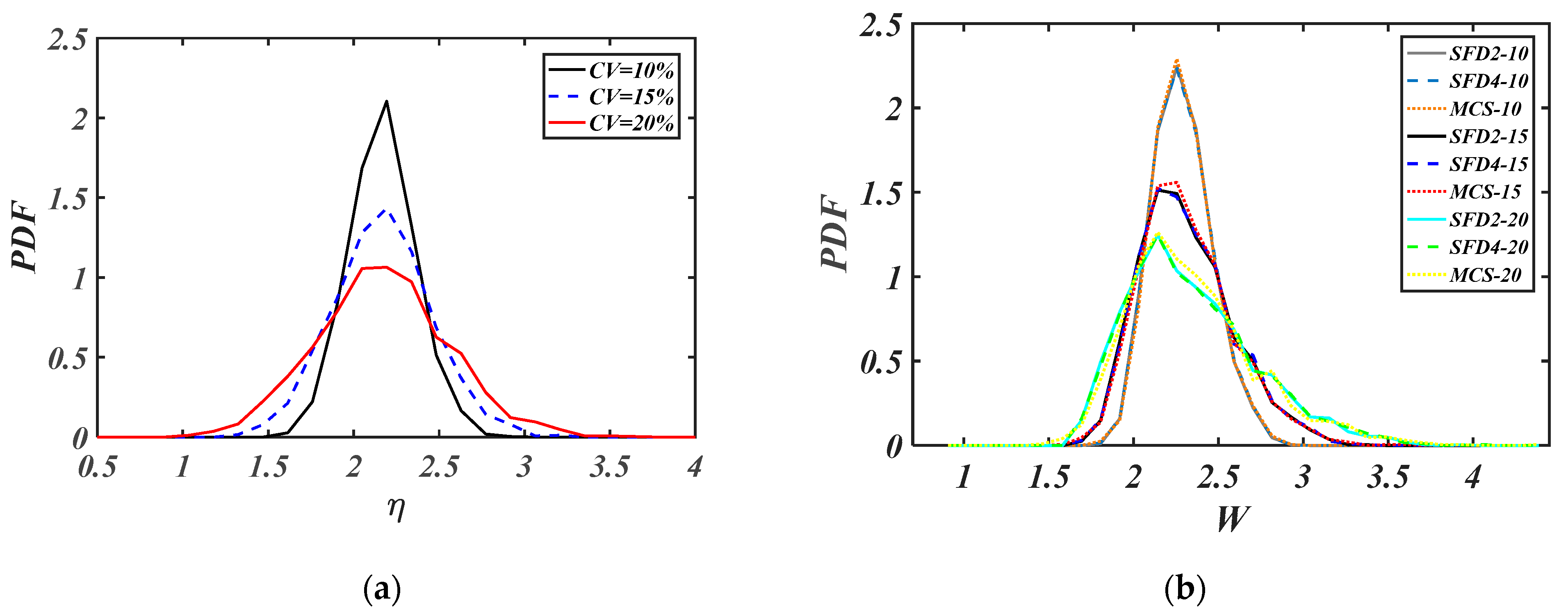
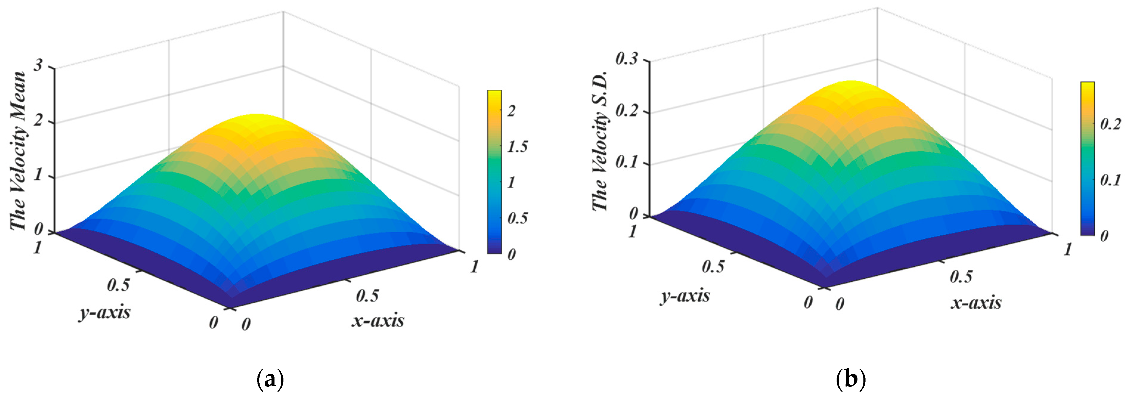
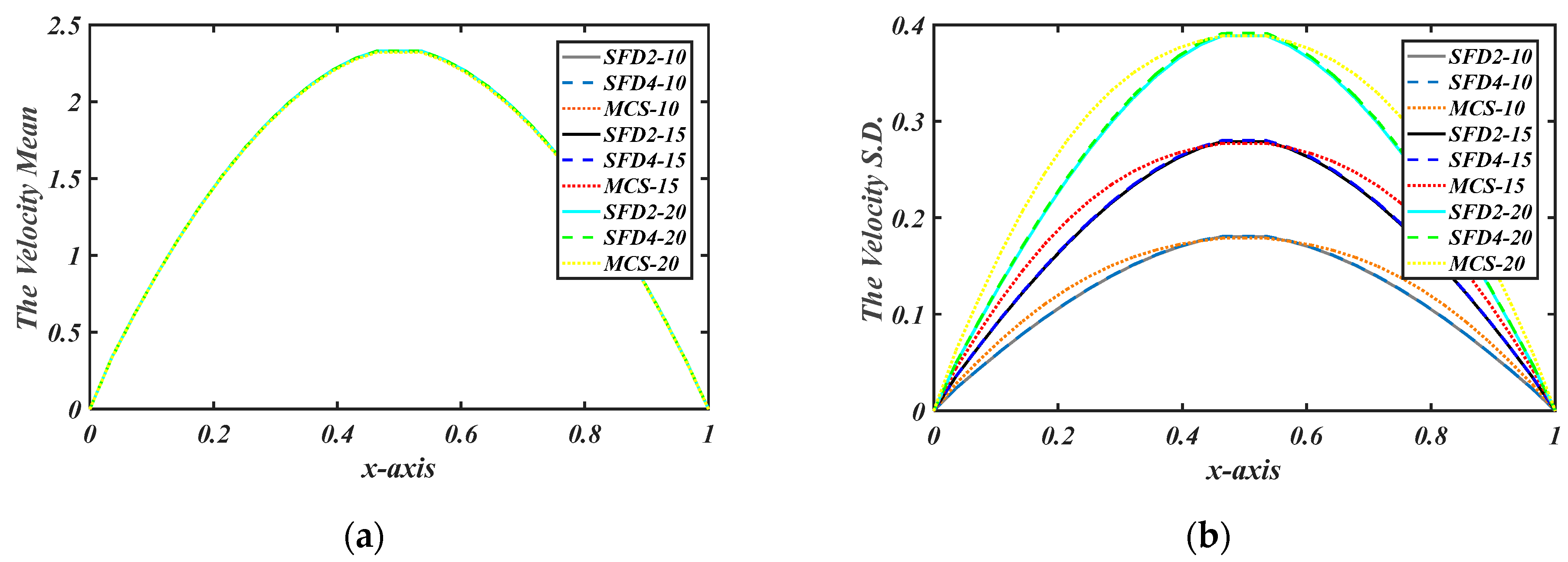
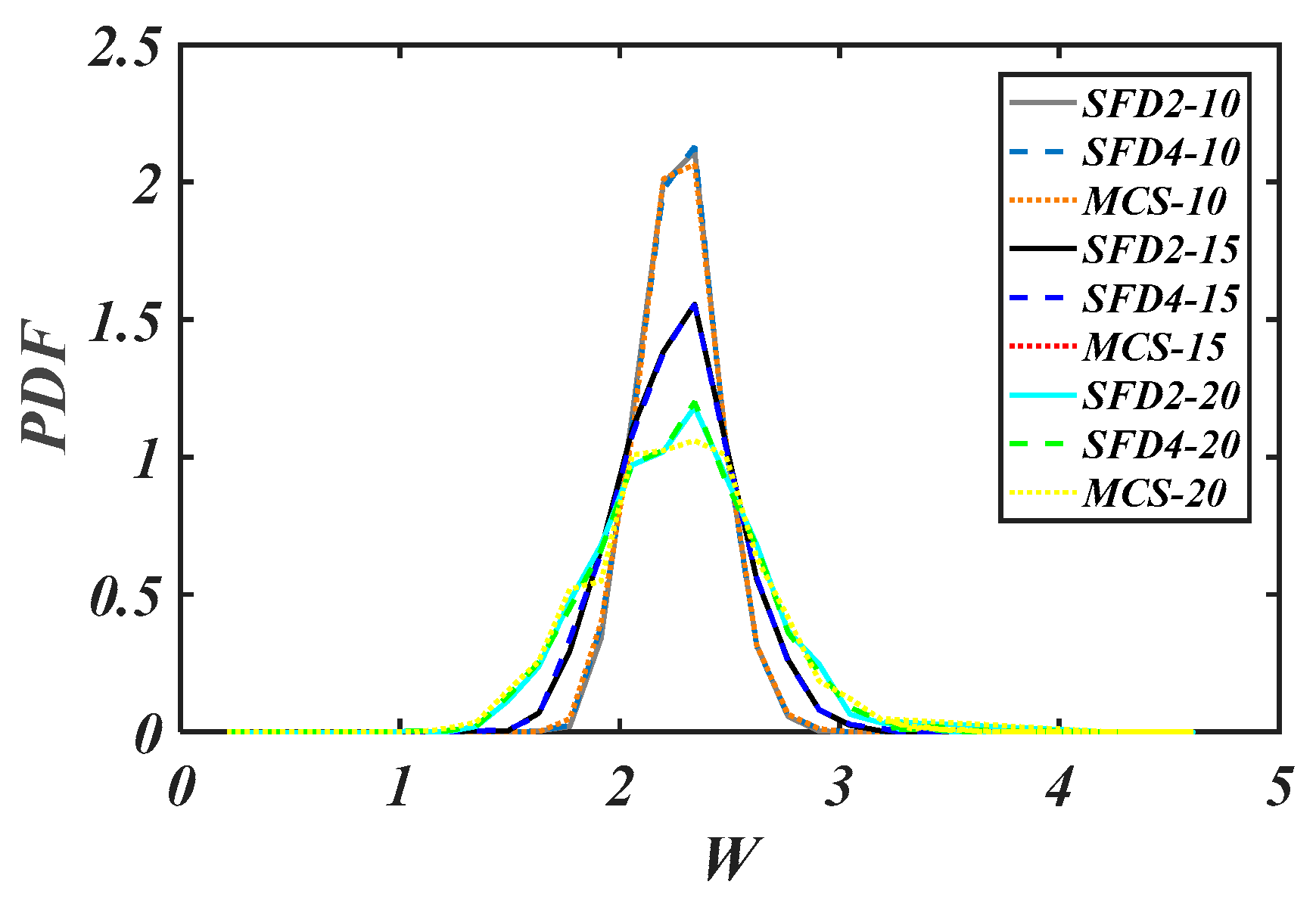
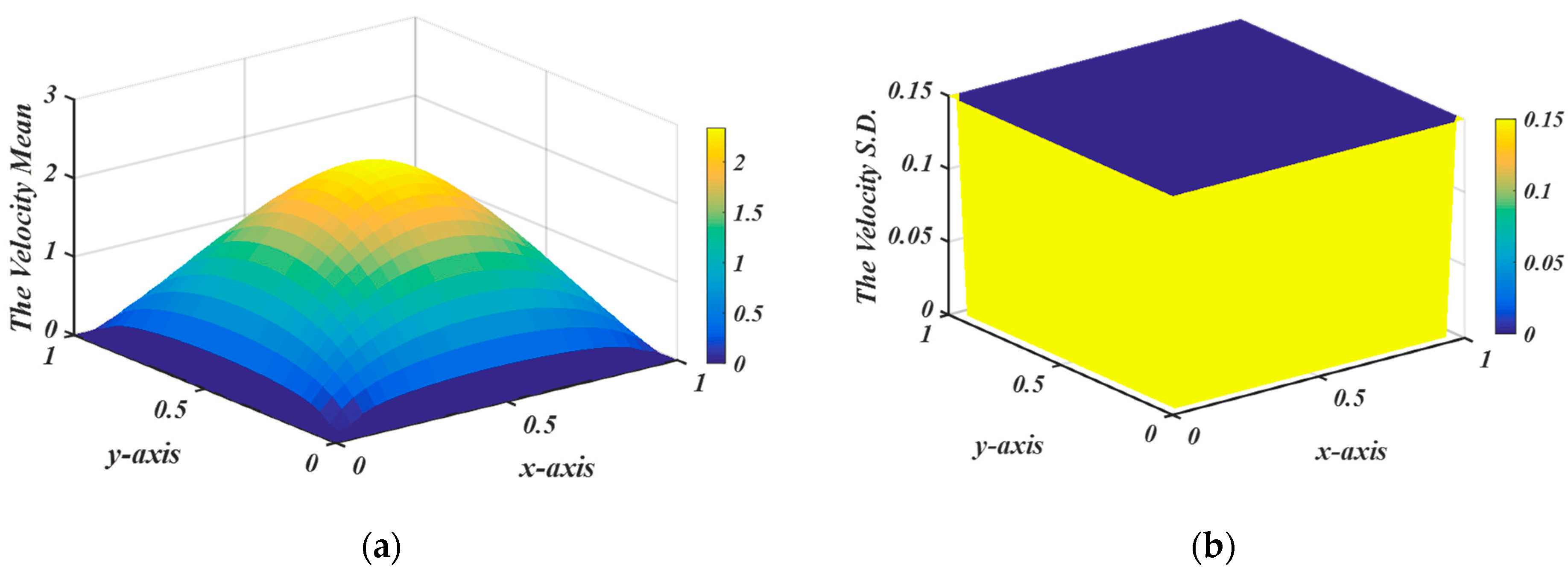
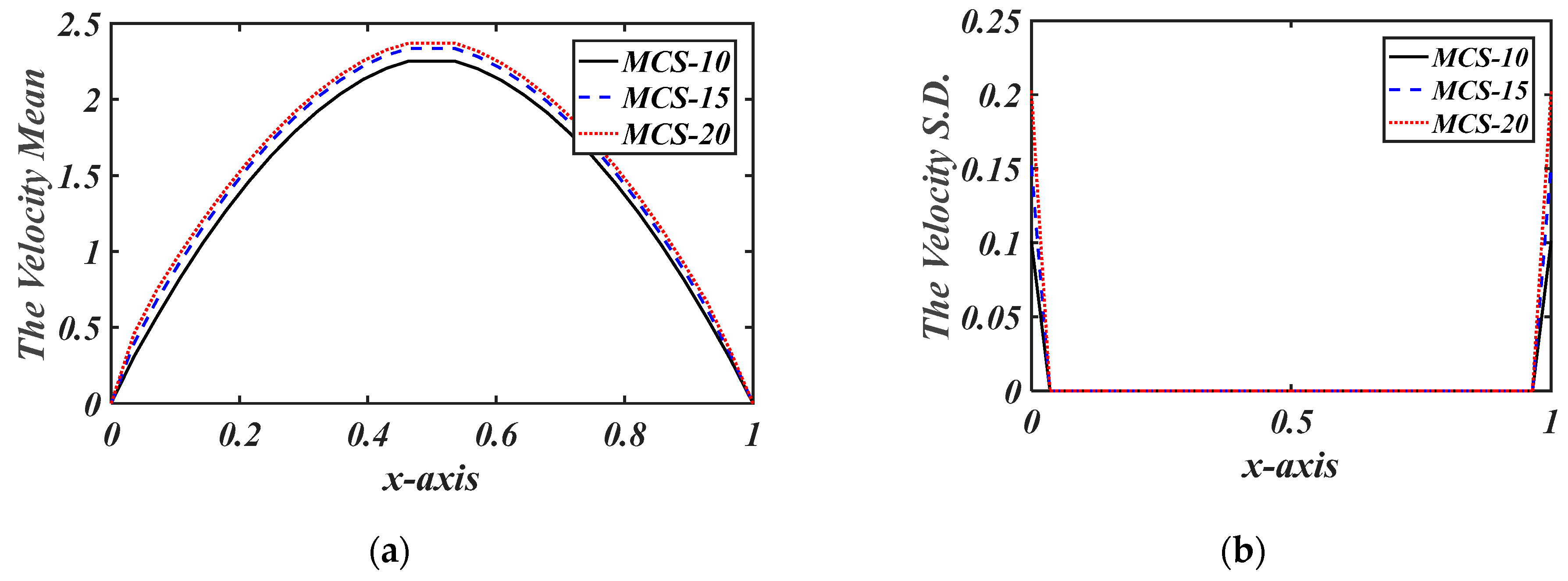
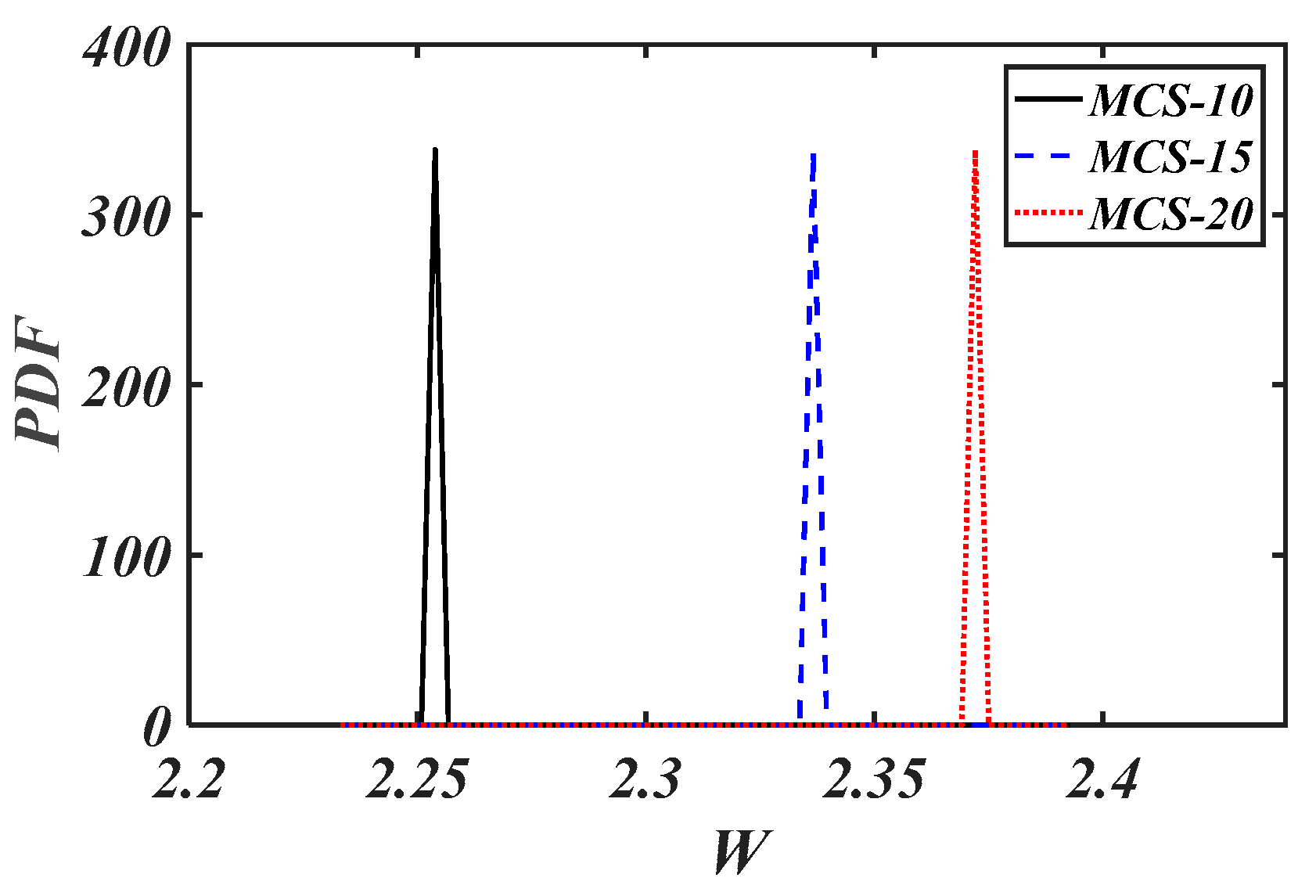
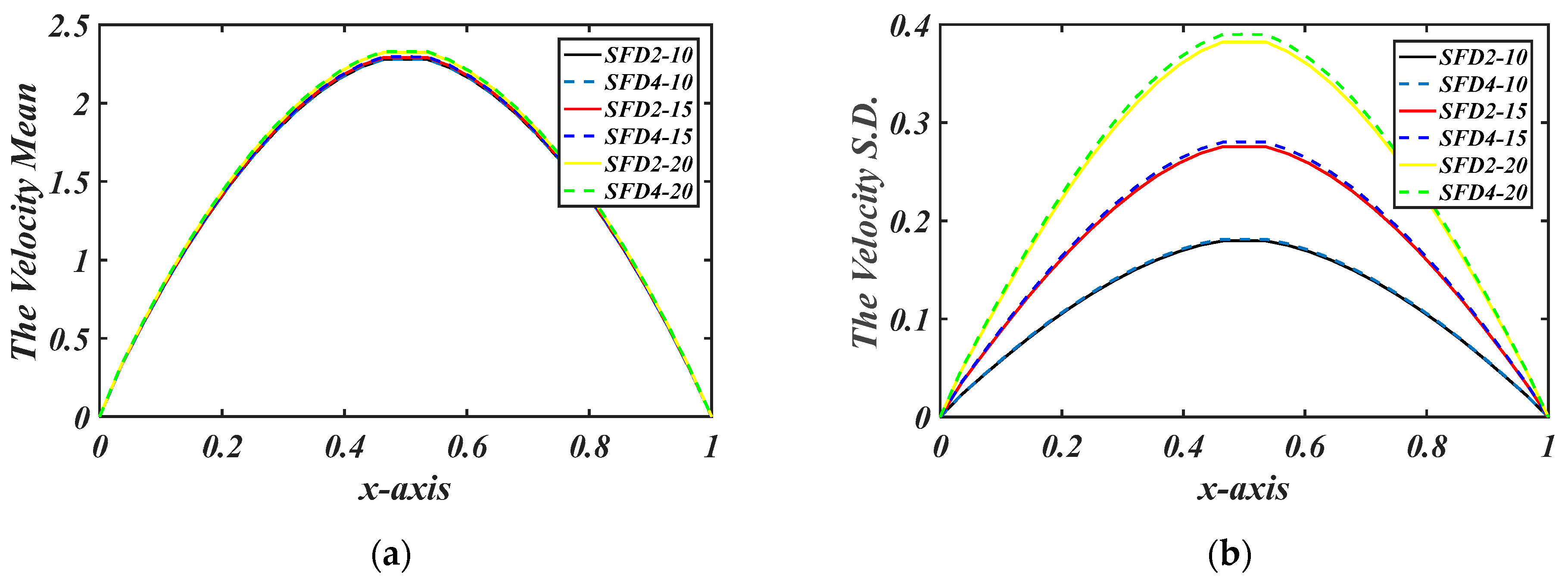
Using SFD2, SFD4, and MCS, the PDFs were computed at each mesh point. The velocity mean, standard deviation (S.D.), approximate minimum, approximate maximum, range, and deterministic velocity are denoted as μ W , σ W , M i n ~ , M a x ~ , R ~ and W D , respectively. Key statistics for the maximum velocity, W m a x at the duct’s center, were tabulated in Table 3, Table 4, Table 5 and Table 6 for Cases I, II, III, and IV, respectively, using the three C values with α = 1 , τ D = 0.3 , and n = 1.5 . Additionally, in Case I, Figure 2a,b display the mean and S.D. across all duct points using SFD4 with CV = 0.15. Figure 3a,b illustrate the mean and S.D. along the x -axis at the midpoint of the y -axis (i.e., y = α / 2 ) for C = 0.1, 0.15, 0.20. Furthermore, Figure 4a illustrates the PDFs of the uncertain viscosity at a specific point (x = y = 1/4, duct’s quarter) as an example for a single realization of the random input, whereas Figure 4b presents the stochastic fluid velocity distributions for three coefficients of variation (CV) across all three solution methods.
For Case I, Table 3 and Figure 2, Figure 3 and Figure 4 reveal several consistent observations. Firstly, all key statistics increase with rising C . The velocity mean, μ W , showed minimal variation, with increases of 0.86%, 1.85%, and 3.28% from W D for the three C values, respectively. Additionally, the ratio σ W / μ W corresponded to 77.1%, 78.9%, and 81.8% of the respective C values, while the approximate minimum and maximum, ( M i n , ~   M a x ~ ) were (78.84%, 130.13%), (70.84%, 153.28%), and (63.95%, 187.45%) of μ W . Moreover, the approximate velocity range, R ~ was 1.1749, 1.9068, and 2.8966 for the three corresponding C values, respectively. This suggests that, despite the small deviation of μ W from W D , the fluid velocity can vary significantly between lower and higher values relative to its mean. Consequently, this highlights the importance for designers to consider these potential low and high velocity extremes.
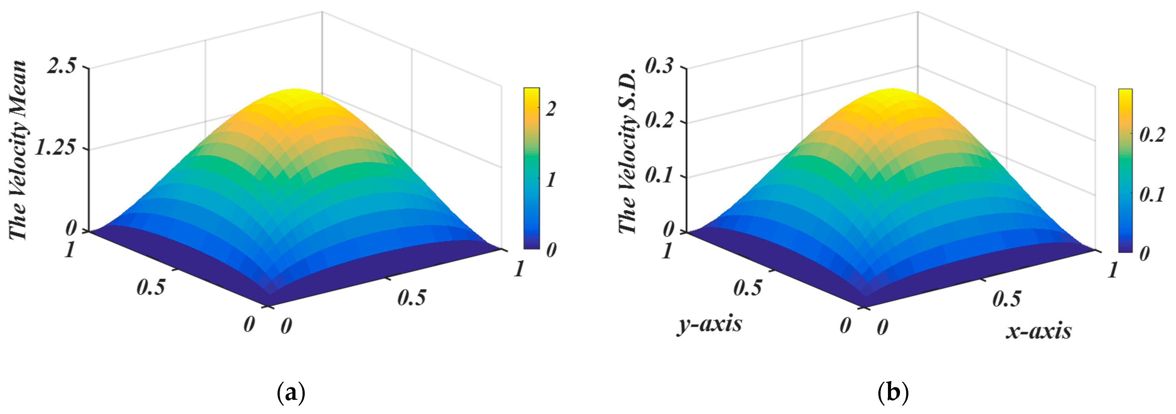
Table 4 and Figure 5, Figure 6 and Figure 7 elucidate the solutions for Case II. Since μ W   /   W D was approximately unity across all solutions, it was evident that the velocity mean, μ W , remained unaffected by the uncertainty in the pressure gradient. Additionally, σ W / μ W exhibited values like those in Case I. The approximate minimum and maximum, ( M i n , ~   M a x ~ ) , were (75.12%, 128.29%), (62.65%, 142.47%), and (50.15%, 156.68%) of μ W , while the approximate range, R ~ , was 1.2050, 1.8075, and 2.4100, lower than Case I for C = 15% and 20%. Subsequently, Table 5 and Figure 8, Figure 9 and Figure 10 detail Case III, which examines uncertain B.C.s. Here, the inherent uncertainty most significantly impacted W m a x , with μ W   /   W D values of 0.9918, 1.0284, and 1.0439. The standard deviation peaked at the boundaries and rapidly diminished, approaching nearly zero at the duct’s center. Moreover, W m a x values were nearly deterministic, with σ W / μ W and R ~ values trending closer to zero.
Case IV, exploring the joint influence of uncertain viscosity and pressure gradient, was evaluated through Table 6 and Figure 11, Figure 12 and Figure 13, chosen for its significant impact on maximum velocity. It consistently displayed the highest velocity standard deviation ( σ W ) and, consequently, the largest range ( R ~ ) values of 1.4355, 2.0256, and 3.0445 across the three coefficients of variation (CV) using SFD4. Moreover, the normalized minimum and maximum velocities ( M i n , ~   M a x ~ ) were (72.62%, 134.69%), (65.49%, 153.13%), and (59.41%, 194.09%) relative to the mean velocity ( μ W ) for the respective CV values. Generally, this case showed the greatest impact on the fluid’s maximum velocity.
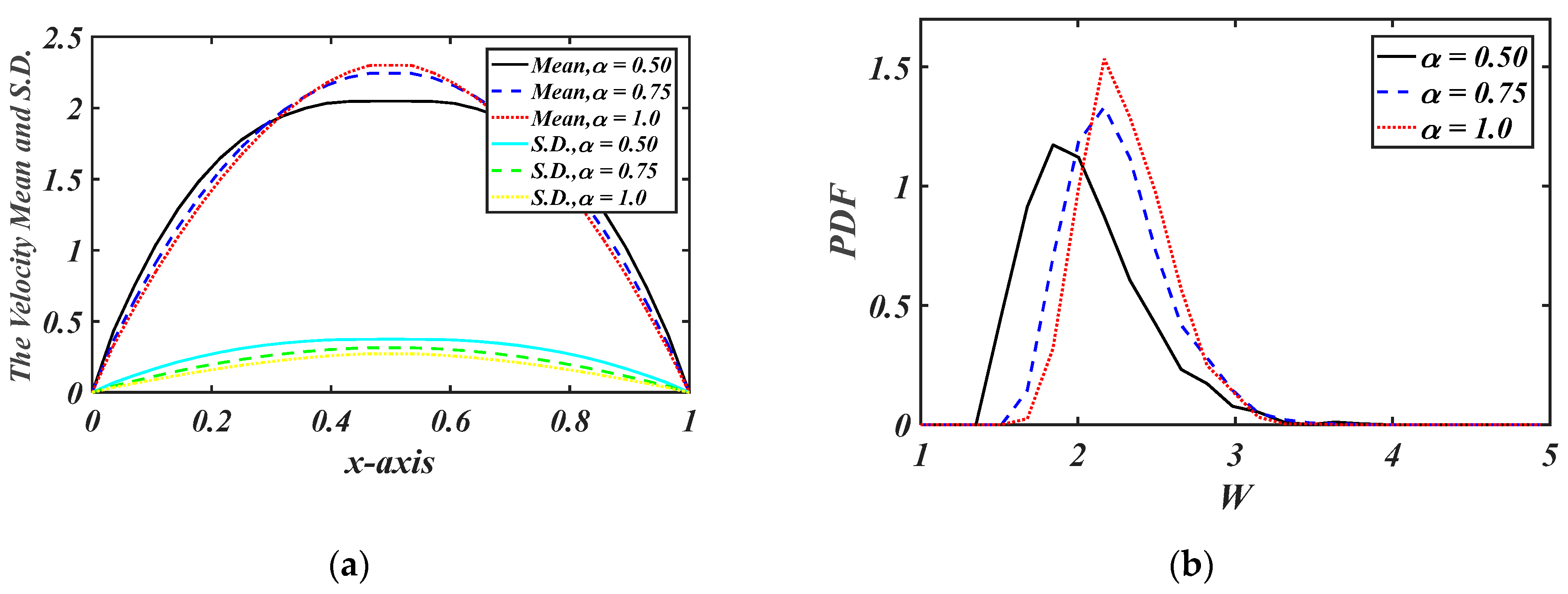
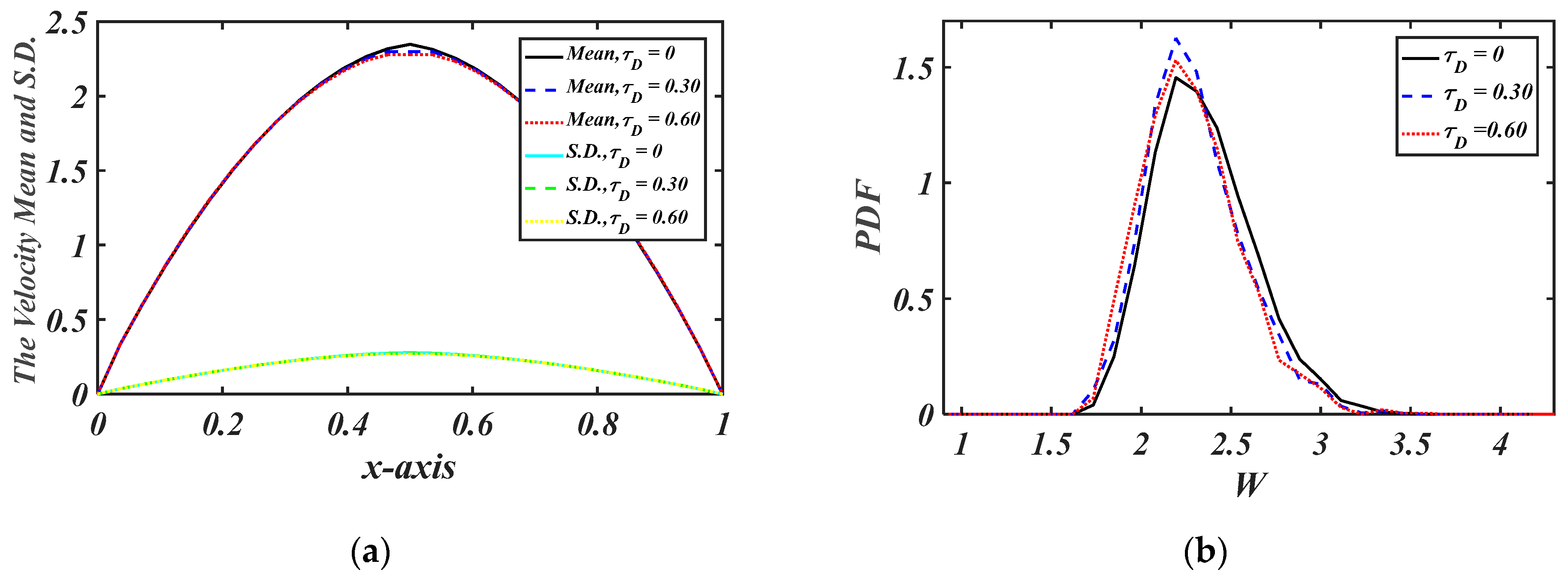
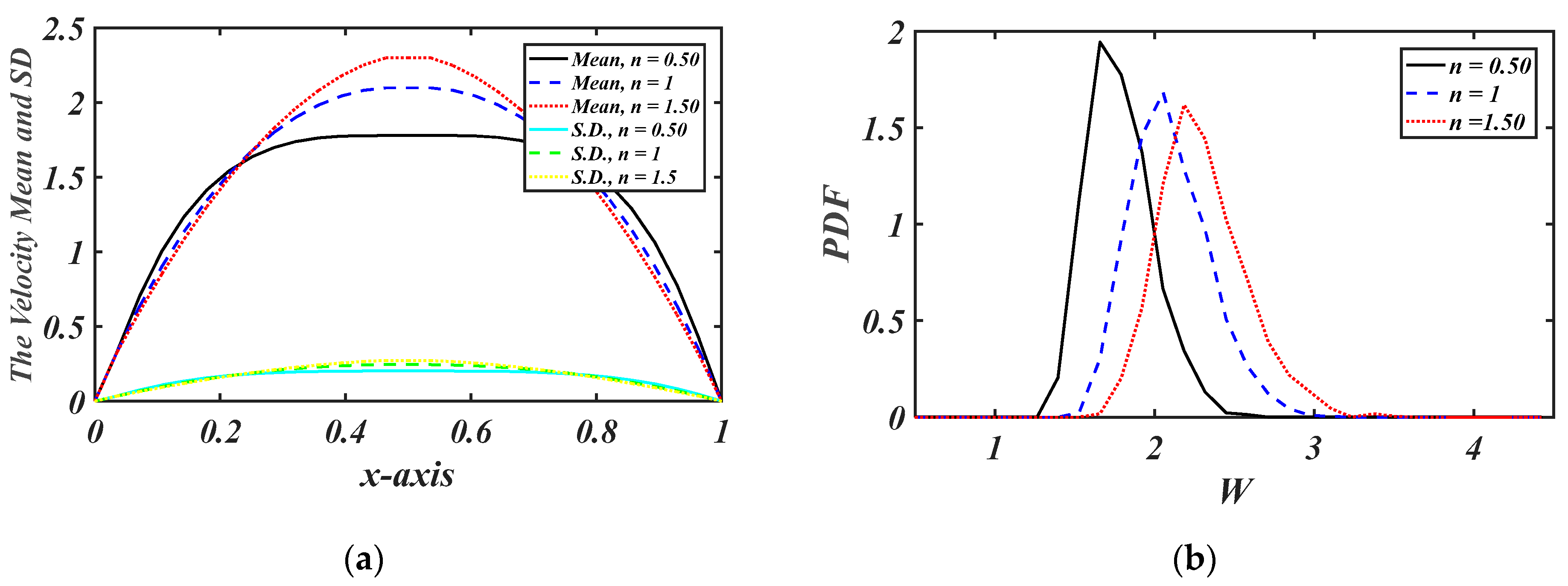
To further explore the fluid behavior, Figure 14, Figure 15 and Figure 16 illustrate the effects of α , τ D and n on μ W , σ W , and the PDF using SFD4 with a CV of 0.15. Specifically, Figure 14a presents μ W and σ W for α = 0.5 , 0.75 , and 1 at n = 1.5 ,   τ D = 0.30 in Case I, while Figure 14b shows the corresponding PDF for W m a x . This analysis indicates that μ W increases with α for 0.3 x 0.7 but decreases outside this range. Additionally, Figure 15a,b highlight the influence of τ D on fluid velocity. With α = 1 and n = 1.5 , τ D = 0 , 0.30 and 0 . 6, the results suggest a minimal effect of τ D on fluid velocity. In contrast, the shear behavior index n exerted the most significant impact. Assuming α = 1 , τ D = 0.30 with n = 0.5 , 1 , and 1.5 , it was found that μ W increases with n for 0.22 x 0.78 but decreases elsewhere, as shown in Figure 16a,b.
Beyond the insights derived from each case, several overarching conclusions emerged. Firstly, with the PDF attainable at all duct points, achievable through both methods utilized here, SFDHC and MCS, a thorough uncertainty quantification is possible. This encompasses all essential statistics, such as the minimum, maximum, mean, S.D., and range. The minimum and maximum delineate the upper and lower limits of fluid velocity fluctuations due to the inherent uncertainty in the parameter under study, offering deeper insight into velocity behavior. Secondly, the accuracy of the SFDHC method improves as the dimensions ( N ) and order ( p ) increase. Given the close agreement between SFD2 and SFD4 results, the SFDHC approach demonstrates rapid convergence. Thirdly, the MCS method involves solving N R independent equations, while SFDHC solves N P C coupled equations. Here, N P C was 6 and 15 for SFD2 and SFD4, respectively, compared to N R = 2 × 10 3 for MCS. This indicates that SFDHC’s computational cost is significantly lower than that of MCS. After constructing the essential matrices, the execution times for the current problem were 15 s for SFD2, 61 s for SFD4, and 14,822 s for MCS, highlighting the significantly reduced computational demand of the SFDHC approach, which is 243 times faster.
Furthermore, the SFDHC method equips engineers with statistical design tools, delivering PDFs and metrics (mean, standard deviation, min/max velocities) to create ducts with safety margins, such as oversized ducts, to prevent drilling blockages or undersized ducts to optimize material use in paint transport. By identifying the fluid behavior index, n as the primary driver of velocity uncertainty (Section 5, Figure 14, Figure 15 and Figure 16), SFDHC guides material selection for stable flow in biomedical and industrial applications. Its computational efficiency (15–61 s vs. 14,822 s for MCS) enables rapid iterative simulations, allowing engineers to test diverse duct geometries and fluid formulations efficiently.

6. Conclusions

This research significantly enhances the stochastic modeling of Herschel–Bulkley (H-B) fluid flow in rectangular ducts by quantifying velocity uncertainties across four scenarios: uncertain apparent viscosity (Case I), pressure gradient (Case II), boundary conditions (Case III), and both viscosity and pressure gradient (Case IV). The stochastic finite difference with homogeneous chaos (SFDHC) method is 243 times faster than Monte Carlo simulation (MCS), yet it retains high accuracy in statistical outputs and probability density functions (PDFs). The method’s rapid convergence, validated by close agreement between SFD2 and SFD4, supports its scalability for complex fluid dynamics simulations. The results demonstrate significant velocity variations in Cases I, II, and IV. For instance, at CV = 20%, the mean velocity ( μ W ) was 2.3348, with minimum and maximum values ranging from 59.41% to 194.09% of μ W ( R ~ = 3.1445). These wide velocity ranges highlight their importance for ensuring robust design in various applications. In contrast, Case III exhibits near-deterministic behavior at the duct’s center, with minimal velocity fluctuations due to boundary effects, underscoring the localized impact of boundary uncertainties. The fluid behavior index ( n ) emerges as the dominant factor influencing velocity, followed by aspect ratio ( α ) and yield stress ( τ D ), providing essential guidance for optimizing duct geometries and fluid formulations. These findings enable robust and reliable uncertainty quantification for chemical processing, food production, and pharmaceutical manufacturing, ensuring safer and more efficient operations under real-world variability. The SFDHC framework’s efficiency and accuracy pave the way for future extensions to energy dissipation, three-dimensional flows, turbulent regimes, or multiphase systems, potentially integrating advanced solvers or machine learning for enhanced scalability.

Author Contributions

Conceptualization, O.H.G.; methodology, O.H.G.; software, O.H.G.; validation O.H.G. and E.A.; formal analysis, O.H.G.; investigation, O.H.G. and E.A.; resources, O.H.G. and E.A.; writing—original draft preparation, O.H.G.; writing—review and editing, O.H.G.; visualization, O.H.G. and E.A.; supervision, O.H.G. and E.A.; funding acquisition, E.A. All authors have read and agreed to the published version of the manuscript.

Funding

The authors extend their appreciation to the Deanship of Scientific Research at Northern Border University, Arar, KSA for funding this research work through the project number NBU-FFR-2025-2768-01.

Data Availability Statement

Data are contained within the article.

Conflicts of Interest

The authors declare no conflicts of interest.

References

  1. Herschel, W.H.; Bulkley, R. Konsistenzmessungen von Gummi-Benzollösungen. Kolloid-Zeitschrift 1926, 39, 291–300. [Google Scholar] [CrossRef]
  2. Nguyen, V.H.; Rémond, S.; Gallias, J.L.; Bigas, J.P.; Muller, P. Flow of Herschel-Bulkley fluids through the Marsh cone. J. Non-Newtonian Fluid Mech. 2006, 139, 128–134. [Google Scholar] [CrossRef]
  3. Sayed-Ahmed, M.E. Laminar heat transfer for thermally developing flow of a Herschel-Bulkley fluid in a square duct. Int. Commun. Heat Mass Transf. 2000, 27, 1013–1024. [Google Scholar] [CrossRef]
  4. Sayed-Ahmed, M.E.; Kishk, K.M. Heat transfer for Herschel-Bulkley fluids in the entrance region of a rectangular duct. Int. Commun. Heat Mass Transf. 2008, 35, 1007–1016. [Google Scholar] [CrossRef]
  5. Sayed-Ahmed, M.E.; Saif-Elyazal, A.; Iskander, L. Laminar flow and heat transfer of Herschel-Bulkley fluids in a rectangular duct; finite-element analysis. Tikrit J. Eng. Sci. 2009, 12, 99–107. [Google Scholar] [CrossRef]
  6. Di Federico, V.; Pinardi, R.; Sgambati, M. Gravity-driven flow of Herschel-Bulkley fluid in a fracture and in a 2D porous medium. J. Fluid Mech. 2017, 821, 59–84. [Google Scholar] [CrossRef]
  7. Vajravelu, K.; Sreenadh, S.; Devaki, P.; Prasad, K.V. Mathematical model for a Herschel-Bulkley fluid flow in an elastic tube. Open Phys. 2011, 9, 1357–1365. [Google Scholar] [CrossRef]
  8. Maiti, A.K. Mathematical modelling on blood flow under atherosclerotic condition. Am. J. Appl. Math. 2016, 4, 324–329. [Google Scholar] [CrossRef]
  9. Maruthi Prasad, K.; Radhakrishnamacharya, G. Flow of Herschel-Bulkley fluid through an inclined tube of non-uniform cross-section with multiple stenoses. Arch. Mech. 2008, 60, 161–172. [Google Scholar]
  10. Rajashekhar, C.; Manjunatha, G.; Basavarajappa, K.S. Peristaltic transport of two-layered blood flow using Herschel-Bulkley model. Cogent Eng. 2018, 5, 1495592. [Google Scholar] [CrossRef]
  11. Liu, R.; Ding, Z.; Hu, K.X. Stabilities in plane Poiseuille flow of Herschel-Bulkley fluid. J. Non-Newtonian Fluid Mech. 2018, 251, 132–144. [Google Scholar] [CrossRef]
  12. Choudhari, R.; Gudekote, M.; Vaidya, H.; Prasad, K.V. Peristaltic flow of Herschel-Bulkley fluid in an elastic tube with slip at porous walls. J. Adv. Res. Fluid Mech. Therm. Sci. 2018, 52, 63–75. [Google Scholar]
  13. Priyadharshini, S.; Ponalagusamy, R. A numerical study on unsteady flow of Herschel-Bulkley nanofluid through an inclined artery with body acceleration and magnetic field. Int. J. Appl. Comput. Math. 2019, 5, 6. [Google Scholar] [CrossRef]
  14. Oberkampf, W.L.; DeLand, S.M.; Rutherford, B.M.; Diegert, K.V.; Alvin, K.F. Error and uncertainty in modeling and simulation. Reliab. Eng. Syst. Saf. 2002, 75, 333–357. [Google Scholar] [CrossRef]
  15. Breuer, H.P.; Petruccione, F. A stochastic approach to computational fluid dynamics. Contin. Mech. Thermodyn. 1992, 4, 247–267. [Google Scholar] [CrossRef]
  16. Mikulevicius, R.; Rozovskii, B. On equations of stochastic fluid mechanics. In Stochastics in Finite and Infinite Dimensions; Birkhäuser: Boston, MA, USA, 2001; pp. 285–302. [Google Scholar] [CrossRef]
  17. Walters, R.A. Hermite polynomial chaos for uncertainty analysis in fluid flow modeling. J. Comput. Phys. 2009, 228, 2988–3005. [Google Scholar] [CrossRef]
  18. Prieto, J.L. Stochastic particle level set simulations of buoyancy-driven droplets in non-Newtonian fluids. J. Non-Newtonian Fluid Mech. 2015, 226, 16–31. [Google Scholar] [CrossRef]
  19. Sochi, T. Deterministic and stochastic algorithms for resolving the flow fields in ducts and networks using energy minimization. Int. J. Mod. Phys. C 2016, 27, 1650036. [Google Scholar] [CrossRef]
  20. De, S.; Kuipers, J.A.M.; Peters, E.A.J.F.; Padding, J.T. Viscoelastic flow simulations in random porous media. J. Non-Newtonian Fluid Mech. 2017, 248, 50–61. [Google Scholar] [CrossRef]
  21. Bedrossian, J.; Blumenthal, J.; Punshon-Smith, S. Lagrangian stochastic models with applications in turbulent transport. J. Fluid Mech. 2020, 898, A25. [Google Scholar] [CrossRef]
  22. Guadagnini, A.; Porta, G.M.; Riva, M.; Bianchi Janetti, I. Quantification of uncertainties of fracture permeability via mud loss information and inverse stochastic modeling. In Proceedings of the 81st EAGE Conference and Exhibition, London, UK, 3–6 June 2019; EAGE: Houten, The Netherlands, 2019. [Google Scholar] [CrossRef]
  23. Galal, O.H. Stochastic velocity modeling of magneto-hydrodynamics non-Darcy flow between two stationary parallel plates. Alex. Eng. J. 2021, 60, 4191–4201. [Google Scholar] [CrossRef]
  24. Galal, O.H. Stochastic Velocity Assessment of Robertson-Stiff Fluids in Rectangular Ducts under Uncertain Parameters and Boundary Conditions. J. Appl. Comput. Mech. 2025. [Google Scholar] [CrossRef]
  25. Rinkens, A.; Verhoosel, C.V.; Jaensson, N.O. Uncertainty quantification for the squeeze flow of generalized Newtonian fluids. J. Non-Newtonian Fluid Mech. 2023, 311, 105154. [Google Scholar] [CrossRef]
  26. Rezaeiravesh, S.; Vinuesa, R.; Schlatter, P. An uncertainty-quantification framework for assessing accuracy, sensitivity, and robustness in computational fluid dynamics. Comput. Methods Appl. Mech. Eng. 2022, 390, 114467. [Google Scholar] [CrossRef]
  27. Al Jaberi, J.; Bageri, B.; Otain, W.; Alsaleem, A.; Adebayo, A.R. Fine-tuning filter cake sealing performance: The role of particle size in hematite weighted water-based drilling fluid. ACS Omega 2024, 9, 21845–21856. [Google Scholar] [CrossRef]
  28. Knio, O.M.; Le Maître, O.P. Uncertainty propagation in CFD using polynomial chaos decomposition. Fluid Dyn. Res. 2006, 38, 616–640. [Google Scholar] [CrossRef]
  29. Gunzburger, M.; Iliescu, T.; Mohebujjaman, M.; Schneier, M. An evolve-filter-relax stabilized reduced-order stochastic collocation method for the time-dependent Navier–Stokes equations. SIAM/ASA J. Uncertain. Quantif. 2019, 7, 1162–1193. [Google Scholar] [CrossRef]
  30. Wang, Q.; Zhang, S.; Zhang, Y.; Fu, J.; Liu, Z. Enhancing performance of nanofluid mini-channel heat sinks through machine learning and multi-objective optimization of operating parameters. Int. J. Heat Mass Transf. 2023, 204, 124204. [Google Scholar] [CrossRef]
  31. Galal, O.H. A proposed stochastic finite difference approach based on homogeneous chaos expansion. J. Appl. Math. 2013, 2013, 950469. [Google Scholar] [CrossRef]
  32. Ghanem, R.G.; Spanos, P.D. Stochastic Finite Elements: A Spectral Approach; Courier Corporation: Mineola, NY, USA, 2003. [Google Scholar] [CrossRef]
  33. Balmforth, N.J.; Frigaard, I.A.; Ovarlez, G. Yielding to stress: Recent developments in viscoelastic fluid mechanics. Annu. Rev. Fluid Mech. 2014, 46, 121–146. [Google Scholar] [CrossRef]
  34. Gao, S.X.; Hartnett, J.P. Non-Newtonian fluid laminar flow and forced convection heat transfer in rectangular ducts. Int. Commun. Heat Mass Transf. 1992, 19, 673–686. [Google Scholar] [CrossRef]
  35. Baranovskii, E.S. The Stationary Navier–Stokes–Boussinesq System with a Regularized Dissipation Function. Math. Notes Acad. Sci. USSR 2024, 115, 670–682. [Google Scholar] [CrossRef]
  36. The MathWorks Inc. MATLAB Version: 9.13.0 (R2022b); The MathWorks Inc.: Natick, MA, USA, 2022; Available online: https://www.mathworks.com (accessed on 5 May 2025).
  37. Syrjala, S. Finite-element analysis of fully developed laminar flow of power-law non-Newtonian fluid in a rectangular duct. Int. Commun. Heat Mass Transf. 1995, 22, 549–557. [Google Scholar] [CrossRef]
  38. Chan, W.K.V. (Ed.) Theory and Applications of Monte Carlo Simulations; BoD–Books on Demand: Norderstedt, Germany, 2013. [Google Scholar] [CrossRef]
  39. Tehrani, A.; Cliffe, A.; Hodder, M.H.; Young, S.; Lee, J.; Stark, J.; Seale, S. Alternative drilling fluid weighting agents: A comprehensive study on ilmenite and hematite. In SPE/IADC Drilling Conference Proceedings; SPE: The Hague, The Netherlands, 2014; pp. 222–239. [Google Scholar] [CrossRef]
  40. Fadl, A.M.; Abdou, M.I.; El-Sayed Ahmed, H.; Wahab Gaber, M.A. Delaminated iron ore (hematite-Barite) as alternative weighting agent to Barite in petroleum drilling fluids engineering operations and mechanism study. Am. Shams Eng. J. 2020, 11, 1317–1337. [Google Scholar] [CrossRef]
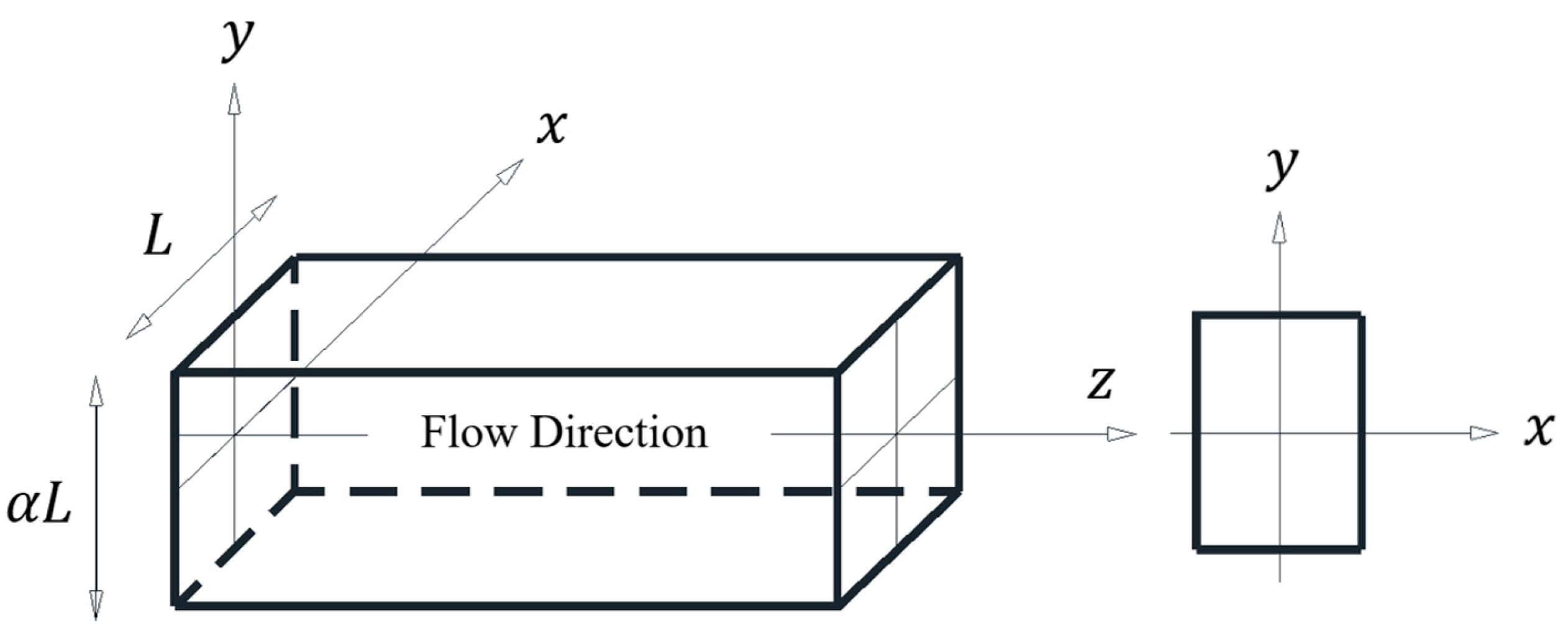
Figure 1. Geometry of the problem.
Axioms 14 00492 g001
Figure 2. (a) The velocity mean using SD4 with CV = 0.15 in case I; (b) the velocity S.D. using SD4 with CV = 0.15 in case I.
Axioms 14 00492 g002
Figure 3. (a) The velocity mean using different methods in case I; (b) the velocity S.D. using different methods in case I.
Axioms 14 00492 g003
Figure 4. (a) The PDF of η for different CV at duct’s quarter in case I; (b) the PDF of W m a x using different methods in case I.
Axioms 14 00492 g004
Figure 5. (a) The velocity mean using SD4 with CV = 0.15 in case II; (b) the velocity S.D. using SD4 with CV = 0.15 in case II.
Axioms 14 00492 g005
Figure 6. (a) The velocity mean using different methods in case II; (b) the velocity S.D. using different methods in case II.
Axioms 14 00492 g006
Figure 7. The PDF of W m a x using different methods in case II.
Axioms 14 00492 g007
Figure 8. (a) The velocity mean using SD4 with CV = 0.15 in case III; (b) the velocity S.D. using SD4 with CV = 0.15 in case III.
Axioms 14 00492 g008
Figure 9. (a) The velocity mean using different methods in case III; (b) the velocity S.D. using different methods in case III.
Axioms 14 00492 g009
Figure 10. The PDF of W m a x using different methods in case III.
Axioms 14 00492 g010
Figure 11. (a) The velocity mean using SD4 with CV = 0.15 in case IV; (b) the velocity S.D. using SD4 with CV = 0.15 in case IV.
Axioms 14 00492 g011
Figure 12. (a) The velocity mean using different methods in case IV; (b) the velocity S.D. using different methods in case IV.
Axioms 14 00492 g012
Figure 13. The PDF of W m a x using different methods in case IV.
Axioms 14 00492 g013
Figure 14. (a) The velocity means and S.D.s for α = 0.5 , 0.75 , and 1, n = 1.5 , τ D = 0.30 in case I; (b) the velocity PDF for α = 0.5 , 0.75 and 1, n = 1.5 , τ D = 0.30 in case I.
Axioms 14 00492 g014
Figure 15. (a) The velocity means and S.D.s for α = 1 , n = 1.5 ,   τ D = 0 ,   0.30 , and 0.60 in case I; (b) the velocity PDF for α = 1 , n = 1.5 ,   τ D = 0 ,   0.30 , and 0.60 in case I.
Axioms 14 00492 g015
Figure 16. (a) The velocity means and S.D.s for α = 1 , τ D = 0.6 , and n = 0.5 ,   1 , and 1.5 in case I; (b) the velocity PDF for α = 1 , τ D = 0.6 , and n = 0.5 ,   1 , and 1.5 in case I.
Axioms 14 00492 g016
Table 1. A comparison of f R e values at α = 1 , τ D = 0 between the current study and previous works for different values of n .
n 0.50.7511.5
Syrjala [37]5.7219.09014.22734.861
Sayed-Ahmed [3]5.7189.07014.23034.880
Present Study5.7759.09514.22834.629
Table 2. A comparison of f R e values for τ D = 0 and different α between the current study and the exact solution by Syrjala [37].
α 10.5
n 1.510.51.510.5
Syrjala [37]34.8609314.227085.7214039.7129215.548065.99867
Present Study34.6285714.228325.7748039.3982215.550076.05751
E r r o r ( % ) 0.6665%0.0087%0.9334%0.7924%0.0129%0.9809%
Table 3. The key statistics for stochastic velocity at the duct’s center in Case I.
CVMethod of Solution μ W μ W / W D σ W σ W / μ W M i n ~ M a x ~ R ~
C = 10 % SFD2-10 2.2848 1.0061 0.1757 0.078 1.8313 2.9501 1.1187
SFD4-10 2.2858 1.0066 0.1761 0.0781 1.8292 2.9512 1.1220
MCS-10 2.2905 1.0086 0.1742 0.0771 1.8058 2.9808 1.1749
C = 15 % SFD2-15 2.3029 1.0141 0.2718 0.1196 1.7129 3.4158 1.7029
SFD4-15 2.3054 1.0152 0.2729 0.1199 1.7115 3.4200 1.7085
MCS-15 2.3129 1.0185 0.2700 0.1183 1.6385 3.5453 1.9068
C = 20 % SFD2-20 2.3298 1.0259 0.3785 0.1647 1.6627 3.9906 2.3279
SFD4-20 2.3346 1.0281 0.3811 0.1654 1.6634 4.0018 2.3384
MCS-20 2.3454 1.0328 0.3785 0.1635 1.4998 4.3964 2.8966
Table 4. The key statistics for stochastic velocity at the duct’s center in Case II.
CVMethod of Solution μ W μ W / W D σ W σ W / μ W M i n ~ M a x ~ R ~
C = 10 % SFD2-102.27091.00000.17580.07841.68142.86271.1813
SFD4-102.27091.00000.17780.07931.68312.88321.2000
MCS-102.26650.99810.18210.08141.70272.90771.2050
C = 15 % SFD2-152.27091.00000.26360.11771.38663.15861.7720
SFD4-152.27091.00000.26670.11901.38923.18931.8001
MCS-152.26440.99710.27320.12221.41863.22611.8075
C = 20 % SFD2-202.27091.00000.35150.15691.09193.45452.3626
SFD4-202.27091.00000.35550.15871.09543.49552.4001
MCS-202.26220.99620.36420.16321.13453.54452.4100
Table 5. The key statistics for stochastic velocity at the duct’s center in Case III.
CVMethod of Solution μ W μ W / W D σ W σ W / μ W M i n ~ M a x ~ R ~
C = 10 % MCS-10 2.2524 0.9918 7.1519 × 10−143.2178 × 10⁻¹⁴ 2.2524 2.2524 0
C = 15 % MCS-15 2.3354 1.0284 3.5093 × 10−141.5228 × 10⁻¹⁴ 2.3354 2.3354 0
C = 20 % MCS-20 2.3706 1.0439 4.6643 × 10−141.9939 × 10⁻¹⁴ 2.3706 2.3706 0
Table 6. The key statistics for stochastic velocity at the duct’s center in Case IV.
CVMethod of Solution μ W μ W / W D σ W σ W / μ W M i n ~ M a x ~ R ~
C = 10 % SFD2-10 2.2863 1.00680.18970.08301.66033.07171.4114
SFD4-102.28711.00710.19210.08401.64513.08061.4355
C = 15 % SFD2-152.31041.01740.29230.12651.52673.53532.0086
SFD4-152.31121.01770.29510.12771.51353.53912.0256
C = 20 % SFD2-202.33171.02680.40640.17431.41134.41513.0038
SFD4-202.33481.02810.41030.17571.38724.53173.1445
Disclaimer/Publisher’s Note: The statements, opinions and data contained in all publications are solely those of the individual author(s) and contributor(s) and not of MDPI and/or the editor(s). MDPI and/or the editor(s) disclaim responsibility for any injury to people or property resulting from any ideas, methods, instructions or products referred to in the content.