Abstract
The Monge–Ampère operator, as a nonlinear operator embedded in parabolic differential equations, complicates the demonstration of maximal regularity for these equations. This research uses the Riesz fractional derivative to connect the Monge–Ampère operator with the fractional Laplacian operator. It is then possible to seek the maximal regularity of the parabolic Monge–Ampère equations by following an approach similar to that used for finding the maximal regularity of the parabolic fractional Laplacian operator. The maximal regularity of nonlocal parabolic Monge–Ampère equations guarantees the existence of solutions in the whole space. Based on these conditions, a modified sliding method, an enhancement of the moving planes method, is employed to establish the monotonicity property of the solutions for the nonlocal parabolic Monge–Ampère equations in the whole space.
Keywords:
maximal regularity; a sliding method; the nonlocal Monge–Ampère equations; monotonicity; whole space MSC:
35B50; 35R11; 35K55; 35K99
1. Introduction
This study focuses on nonlinear equations that incorporate the nonlocal parabolic Monge–Ampère equations, which are defined as
and therein, we assume that the function f belongs to the space , with
for any satisfying ; the term denotes the Cauchy principal value. Here, A represents a positive definite square matrix, denoted as . The constraints and collectively imply that is bounded above by . Further details regarding the nonlocal Monge–Ampère operator can be found in [1].
For the integral presented in (1) to be well defined, we impose the condition that u belongs to the space and is locally , where
The space is the space of functions such that the semi-norm is
for some and thus for all . This space is well suited for nonlocal fractional operators because it controls the growth and the regularity of the function in a way that is compatible with the nonlocal nature of the integral in the definition of .
The space consists of functions that are locally and whose first-order derivatives are locally Lipschitz continuous. That is, for any compact set , there exists a constant such that for all ,
For a function , the integral (2) is well defined. The local regularity ensures that the integrand behaves nicely in a neighborhood of x. The condition guarantees that the integral converges at infinity.
The form of the nonlocal Monge–Ampère operator presented in Equation (1) is motivated by several deep connections in analysis, probability, and differential geometry. From theoretical motivation, the classical Monge–Ampère equation arises in optimal transport and differential geometry, where it relates the determinant of the Hessian of a convex function to a given measure. The nonlocal version in Equation (1) extends this by replacing the local Hessian with a nonlocal fractional operator, inspired by the fractional Laplacian , with the following relationship:
represents the fractional Laplacian, which is defined here as
where ; the normalization constant in (3) arises from the Fourier transform definition of the fractional Laplacian and ensures consistency with the standard Laplacian as . The explicit expression for is
stands for the Cauchy principal value, which is defined as
where is the ball of radius centered at x. This limit excludes a small neighborhood around the singularity and then takes the limit as the neighborhood shrinks to zero. More explanations for the normalization constant and Cauchy principal value about the fractional Laplacian can be found in [2,3]. Equations featuring the fractional Laplacian (3) have been extensively studied by numerous researchers, as evidenced in [4,5,6,7,8,9,10] and the cited literature. The nonlocal nature of the fractional Laplacian introduces substantial challenges in its analysis. To address these challenges, the method of moving planes has been utilized to explore the qualitative characteristics of solutions to equations involving nonlocal operators, as referenced in [11,12,13].
In this study, a direct sliding method is utilized to handle the nonlocal Monge–Ampère operator. The well-known sliding method was initiated by Berestycki and Nirenberg [14,15,16] to analyze the qualitative properties of positive solutions for local elliptic equations. Subsequently, Wu and Chen [17] refined this approach into a direct sliding method, which has demonstrated its utility in various applications, including deducing monotonicity, one-dimensional symmetry, uniqueness, and the nonexistence of solutions for elliptic equations and systems involving fractional Laplacians and p-Laplacians. For further details, refer to [18,19,20,21], with an extensive survey available in [22]. This direct method circumvents the necessity for the classical extension techniques outlined in [4] and addresses challenges posed by the nonlocality of fractional operators. For example, the direct method of moving planes relies on local comparisons (e.g., maximum principles for local PDEs); using the sliding method, one can slide u and use the fact that u decays at infinity to derive monotonicity or symmetry. The direct method of moving planes requires constructing auxiliary functions (e.g., ) and analyzing their critical points, while the sliding method often reduces to showing that u is monotone in a certain direction. For u defined on , sliding u in the direction and comparing with is more straightforward. The direct method of moving planes typically requires the domain to be bounded or symmetric to apply the maximum principle; for unbounded domains (e.g., ), the method may not directly apply, and the direct sliding method naturally extends to unbounded domains by using the decay properties of u at infinity. Furthermore, the direct sliding method can be utilized to extend and validate Gibbons’ conjecture within the context of other fractional elliptic equations that incorporate various nonlocal operators (see [23,24,25,26,27]).
In [28], Du and Wang employed the method of moving planes to establish the monotonicity of positive solutions for nonlocal parabolic Monge–Ampère equations as
in the half-space. In this study, the direct sliding method is applied to demonstrate the monotonicity of positive solutions for nonlocal parabolic Monge–Ampère equations, which are defined as
in the whole space. When calculating (1), the integrand
is well behaved at infinity due to the condition . The local regularity of functions in ensures that the function u and its first-order derivatives are well behaved in any compact subset of . This is important for the time derivative term . In [28], Du and Wang demonstrated that the fractional Monge–Ampère operator is strictly elliptic, which allowed them to apply the well-known regularity results for uniformly elliptic operators. In contrast to the typical research focusing on the regularity aspects of fractional Monge–Ampère operators such as in [29], this work delves into the maximal regularity properties of such operators. To accomplish this objective, the methodology introduced by Liu (2024) in [30] is employed, which entails ensuring that the norm of the spatial operator remains below 1. Nevertheless, owing to the nonlocal characteristic of the Monge–Ampère operator, the primary hurdle resides in devising strategies to enforce this norm constraint. Traditionally, researchers might posit the uniform convergence and boundedness of the solution u to address such challenges. In this article, it is precisely this approach that has been employed. Section 3 provides a more detailed exposition.
2. Basic Setup and Main Results
The present work adopts a strategy involving the estimation of singular integrals associated with the nonlocal parabolic Monge–Ampère equations, which are conducted along a sequence of points approximating the maximum. The inspiration for these ideas primarily stems from the research conducted in [31], our objective is to establish the subsequent theorem.
Theorem 1.
Let be a solution of
with condition
and with assumption
Suppose that the function is continuous and exhibits nonincreasing behavior in the vicinity of . Additionally, assume that u is uniformly continuous. Under these conditions, u must be strictly monotonically increasing with respect to the variable , and it depends solely on .
Let us denote the vector x as
For every belonging to the set of real numbers , we define
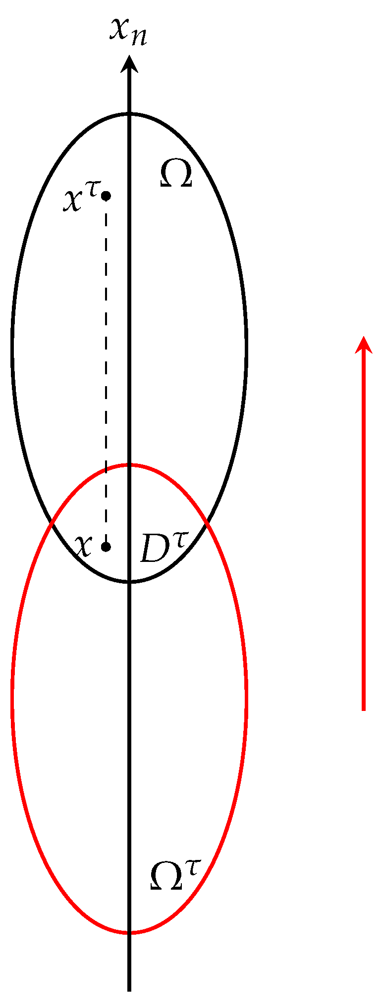
Consider as a bounded region within , exhibiting convexity along the axis. By sliding downward units, we obtain , which is shown in Figure 1:
Define
and
Suppose constitutes a positive solution to the equation given by (4). We then proceed to compare the magnitudes of with
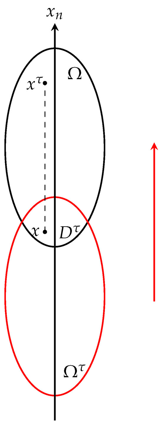
Figure 1.
Sliding method.
Let
Our proof is structured into two distinct phases:
The first step: Begin sliding downward by τ units along the axis.
So then,
The work shall demonstrate that, provided that is sufficiently near to , or equivalently when attains a sufficiently large magnitude, the set exhibits a narrow characteristic, which implies that
The second step: Decrease τ as long as holds to its limiting position.
This work aims to demonstrate that the limiting position corresponds to . In the second step, the proof will be divided into two cases: one is , and the other is . In both cases, it will be shown that the limiting position is . After the second step has been completed, it will be proven that , . Consequently, this concludes the demonstration of the monotonicity property for the solutions of parabolic Monge–Ampère equations across the entire space. The concluding section will establish that the function is solely dependent on the variable .
3. Maximal Regularity of Nonlocal Parabolic Monge–Ampère Equations
This section utilizes the theorem proposed by Liu (2025) [10] to substantiate the existence of solutions for nonlocal parabolic Monge–Ampère equations.
Theorem 2.
Let , and assume that is a classical solution of
and then, the solution of (7) satisfies the - maximal regularity estimate:
for any . This is because , and is dense in .
In distribution theory, even if a function is not differentiable in the classical sense, its derivatives can still be defined as distributions or generalized functions. For a function u, its first-order derivatives are Lipschitz continuous, which implies they are absolutely continuous and differentiable almost everywhere. Although may not be differentiable at isolated points, we can define as a distribution derivative or a weak derivative. If for all test functions , the following equation
holds, then for a function u, the existence of such can be proven, and it is related to the Lipschitz continuity of . Since is Lipschitz continuous, there exists a constant L such that for all , we have
This continuity ensures that the variation of is bounded, allowing us to define its distribution derivatives.
Maximal regularity is a powerful tool in the theory of partial differential equations. It provides a quantitative way to measure the regularity of solutions of PDEs in terms of the regularity of the right-hand side of the equation. While the basic well-posedness results (existence, uniqueness, and continuous dependence on f) only tell us that a solution exists and is unique for a given f, the maximal regularity estimate provides a precise quantitative relationship between the solution and the right-hand side. It tells us how the regularity of the solution is controlled by the regularity of f. For example, if f is in a certain - space, then we know exactly how the - norms of and are bounded in terms of the - norm of f.
The demonstration of Theorem 2 is grounded in the proof of the maximal regularity for parabolic fractional Laplacian equations as presented in [10]. The immediate priority is to approximate the form of the Monge–Ampère operator (1) to the form of the fractional Laplacian (3) in a certain way.
In an isotropic case where (the identity matrix), the nonlocal Monge–Ampère operator simplifies to
This is precisely the fractional Laplacian , evaluated at a fixed time t.
For general matrices A with , the nonlocal Monge–Ampère operator incorporates anisotropic effects. The transition between nonlocal Monge–Ampère operators and fractional Laplacians can be explored through the lens of the Riesz fractional derivative. The Riesz fractional derivative is a well-known alternative definition of the fractional Laplacian. For a function , the Riesz fractional derivative of order in n-dimension is defined in terms of the Fourier transform. If is the Fourier transform of , the Riesz fractional derivative is given by
where , and . In Fourier space, the Riesz fractional derivative corresponds to multiplication by . For the nonlocal Monge–Ampère operator, the Fourier symbol would involve an infimum over all possible "anisotropic" symbols of the form , where A is a matrix with :
The Fourier transform of homogeneous equation
is
and we derive
for some constant and take as the eigenvalue so that (11) forms a semi-group. Then, the process of finding the maximal regularity of the nonlocal parabolic Monge–Ampère problem could refer to the nonlocal parabolic fractional Laplacian equations in [10]. The proof hinges on leveraging the - maximal regularity properties of solutions to heat equations. This approach is justified because the Fourier transforms associated with heat equations exhibit structural parallels to those of fractional Laplacians. Furthermore, fractional Laplacians share a functional form akin to the Riesz fractional derivative, which bears resemblance to the nonlocal Monge–Ampère operators. A comprehensive account of the proof is provided in Theorem 1 of [10].
In the reference [30], Liu succinctly outlined the fundamental logic and principles dictating the existence of maximal regularity for both parabolic and hyperbolic differential equations. Based on the information in this reference, we can substantiate that the prerequisite for achieving maximal regularity in parabolic differential equations is that the eigenvalues of the operator corresponding to spatial variables are less than 1. In (8), we observe that as and , could be bounded by 1; yet, when is not adequately large or t takes a negative value, the following criterion needs to be satisfied to ensure that the eigenvalues of the nonlocal Monge–Ampère operator remain less than 1:
The condition (12) implies that , and combining this with , we have
which leads to
and is equivalent to stating that
To satisfy (12) and (13), we might use norm (maximum value) bounds on to control the eigenvalues of ; for example, in (5) and (6), we have
and
to control the growth of at different points, thereby regulating the eigenvalues of the nonlocal Monge–Ampère operator (9). With the above conditions on u, by employing the sliding technique, we deduce the monotonic behavior of the solutions pertaining to nonlocal parabolic Monge–Ampère equations throughout the entire space .
4. Monotonic Characteristics of Solutions Within
This section elaborates on the comprehensive demonstration of Theorem 1 utilizing the sliding method. Our proof is structured into two distinct stages.
Step 1. It is the aim to demonstrate that, provided attains a sufficiently large value,
Otherwise, if (16) is not satisfied,
and consequently, there is a sequence satisfying the condition that
Let . Given that approaches A as tends to , it follows that there exists a positive constant satisfying
Set
Given that we possess
and
Subsequently, there is a pair fulfilling the condition that
Therefore,
This is because we have
Therefore,
According to the definition provided for , it follows that
We also have
The final inequality at the lower end is valid, owing to .
Therefore,
in which c represents a positive constant associated with .
Upon considering scenarios where attains a sufficiently large value, the following two possibilities emerge:
- The value of approximates 1;
- The value of approximates .
Given the inequality in the first scenario, both and are close to 1. Conversely, in the second scenario, both and are close to . Consequently, regardless of the scenario, we can leverage the monotonicity property of f to establish that
Consequently, it follows that
Thus, we derive
A contradiction is reached, thereby confirming the validity of (16).
Step 2. The inequality (16) serves as an initial condition, enabling us to initiate the sliding process. Subsequently, we progressively reduce the value of until is satisfied at its limiting position. We then define
Within this section, our objective is to demonstrate that .
Otherwise, we have . Initially, this work establishes the proof for
Should (19) fail to be satisfied, it follows that
Then, a sequence exists, where each element is contained within , satisfying the following condition:
Denote . Let be defined as
So, . Set up
Consequently, a sequence can be identified, which converges to 0, fulfilling the condition that
Set
Given that
it can subsequently be established that there exists in , satisfying
Analogous to the demonstration provided in Step 1, from one perspective, we observe that
Conversely, in accordance with the definition of , it follows that
Let
Given that the function u exhibits uniform continuity, we can invoke the Arzelà–Ascoli Theorem to conclude that
As k approaches infinity, leveraging the continuity of the function f and drawing upon the results from Equations (21) and (22), we arrive at the conclusion that
It follows that
Given that the sequence is bounded, we obtain that
For every natural number m, it holds that
Choose to be sufficiently negative and m to be sufficiently large. Under these conditions, we observe that approaches , while approaches 1. This scenario leads to a contradiction. Consequently, Equation (19) must hold true.
Subsequently, this work shall demonstrate the existence of a positive constant satisfying
Based on Equation (19), we can assert the existence of a sufficiently small for which
At this point, it suffices to establish the proof for the case where as
If (25) does not hold, then
We can identify a sequence satisfying , where . Given the conditions, it follows that the sequence is bounded. Define . Then, there exists a sequence with , along with points and , such that
Similarly to previous steps, on the one hand, it holds that
On the other hand,
where .
As k tends to infinity, we observe that approaches 0. This leads to a contradiction, and we consequently arrive at Equation (23), which is in conflict with the definition of . Hence, we deduce that .
To conclude, the work shall demonstrate that the function u is strictly increasing with respect to the variable and that depends solely on .
It has been established that
Suppose that there exists a point in satisfying . In such a case, constitutes the maximum point of the function over the domain . Consequently,
On the one hand,
On the other hand,
The penultimate inequality is valid because is nonpositive across , and specifically negative within the neighborhood .
As approaches 0, it follows that
This leads to a contradiction. Consequently, we obtain
Subsequently, this work aims to demonstrate that the function is solely dependent on the variable .
Should we substitute with , the reasoning remains valid following the preceding methodology. Here, represents an arbitrary upward-pointing vector with . By employing analogous reasoning to that utilized in Step 1 and Step 2, we can deduce that, for every such vector ,
As approaches 0, and leveraging the continuity of the function u, we can conclude that for any arbitrary vector satisfying ,
By replacing by , we can obtain that for arbitrary with ,
Equation (26) implies that the function u does not depend on the variables . As a consequence, we can express as .
This establishes the validity of Theorem 1.
5. Illustrative Numerical Examples
5.1. Illustrative Example of Applying Theorem 1 in Numerical Methods
Referenced from [32,33] in image segmentation, consider a two-dimensional image domain . Let represent the phase variable, where indicates that the pixel x belongs to the object of interest, and indicates that it belongs to the background.
The function can be chosen as , where is a small parameter, and is a double-well potential. Near , is nonincreasing.
According to Theorem 1, if we consider the image domain in a coordinate system where one of the axes (say ) is perpendicular to the boundary between the object and the background, then u is strictly increasing with respect to and depends only on . In numerical simulations, this property can be used to simplify the computational domain. For example, if we know that the solution is one-dimensional in the direction perpendicular to the object–background boundary, we can reduce the two-dimensional image segmentation problem to a one-dimensional problem along the relevant axis, which significantly reduces the computational cost.
5.2. Illustrative Example of Applying Nonlocal Monge–Ampère Operator in Geometry Flow
In the perspective of fractional calculus and nonlocal geometry, the operator can be interpreted as a fractional Hessian determinant, where the principal value integral generalizes the second derivative to a nonlocal setting. This parallels the manner in which the fractional Laplacian extends the classical Laplacian to nonlocal frameworks. Such operators naturally arise in the study of nonlocal minimal surfaces [34], where the minimization of a nonlocal energy functional leads to surfaces with geometric properties distinct from their classical counterparts. Additionally, geometric flows driven by fractional curvatures, such as the fractional mean curvature flow, provide further contexts that play a central role.
This study examines the numerical approximation of surface evolution under fractional mean curvature flow using the method in [35], which describes the evolution of a surface , with certain initial condition , moving with velocity
where H denotes the fractional mean curvature, and n is the normal vector of the surface. We use identity , where and denote the nonlocal Monge–Ampère operator and identity map on surface . The fractional mean curvature flow can also be written as
By utilizing the formulation in (27), we use the parametric Finite Element Methods (FEMs) for approximating surface evolution under fractional mean curvature flow. Assuming that is already approximated by a piecewise triangular surface , find a parametrization of surface through a finite element function , which is determined by some weak formulation of (27). More methodology and proof can be checked in [35].
Here, the study presents a simplified approach to parametric FEMs. A 3D cubic mesh was generated using a parameterized approach, where the number of points along each dimension is controlled by the parameter n. The vertices v of the mesh are defined as
where are uniformly spaced points in the interval . The faces of the mesh are constructed by connecting adjacent vertices to form cubes. The nonlocal Monge–Ampère operator is discretized using a Gaussian weighting scheme. For each vertex , the operator computes a weighted average of its neighboring vertices. The weights are defined as
where defines the standard deviation of the Gaussian weighting function, and it controls the range of the nonlocal interaction. The weights are normalized to ensure the sum is one as
The nonlocal update for each vertex is computed as
where represents the displacement due to the nonlocal operator.
The vertices are updated using an explicit Euler time integration scheme:
where is the time step size for the explicit Euler method. The n values are chosen as number of points along each dimension of the cube, in our case .
Visualization
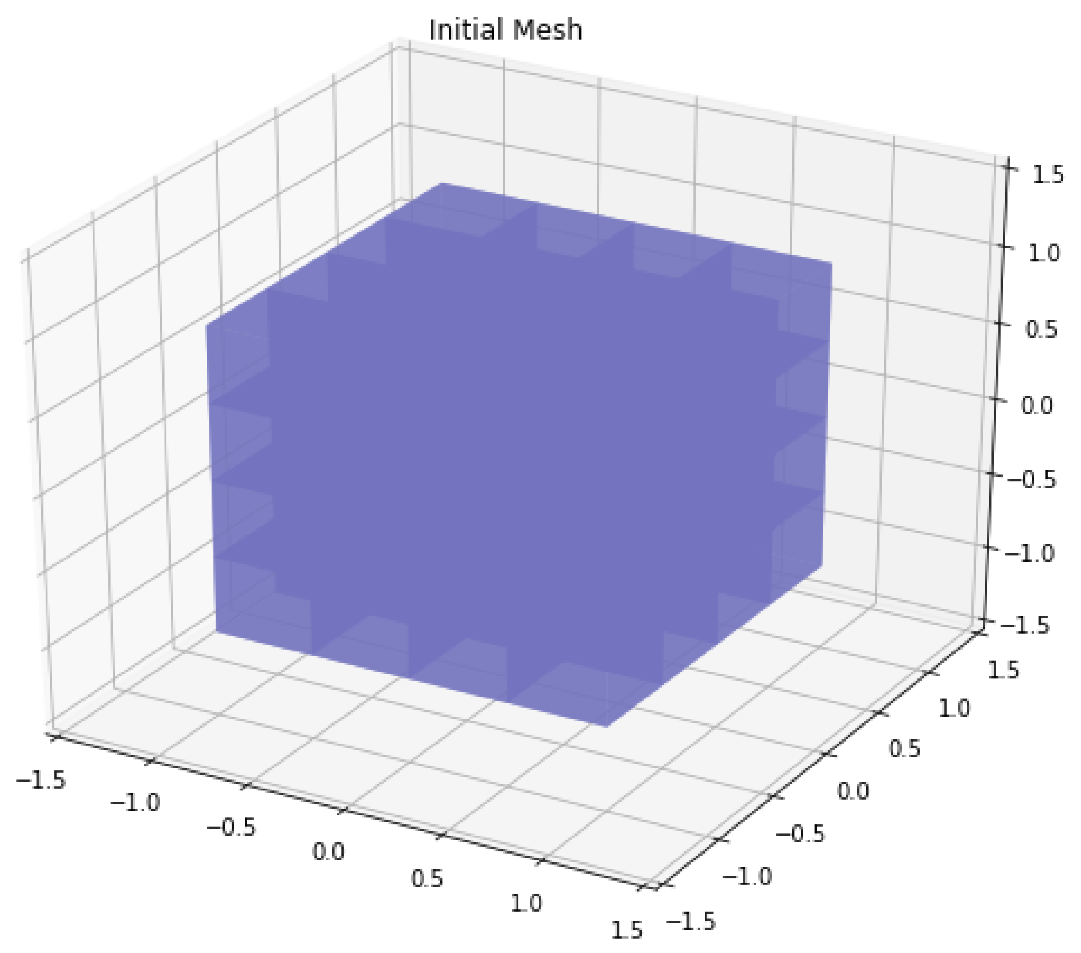
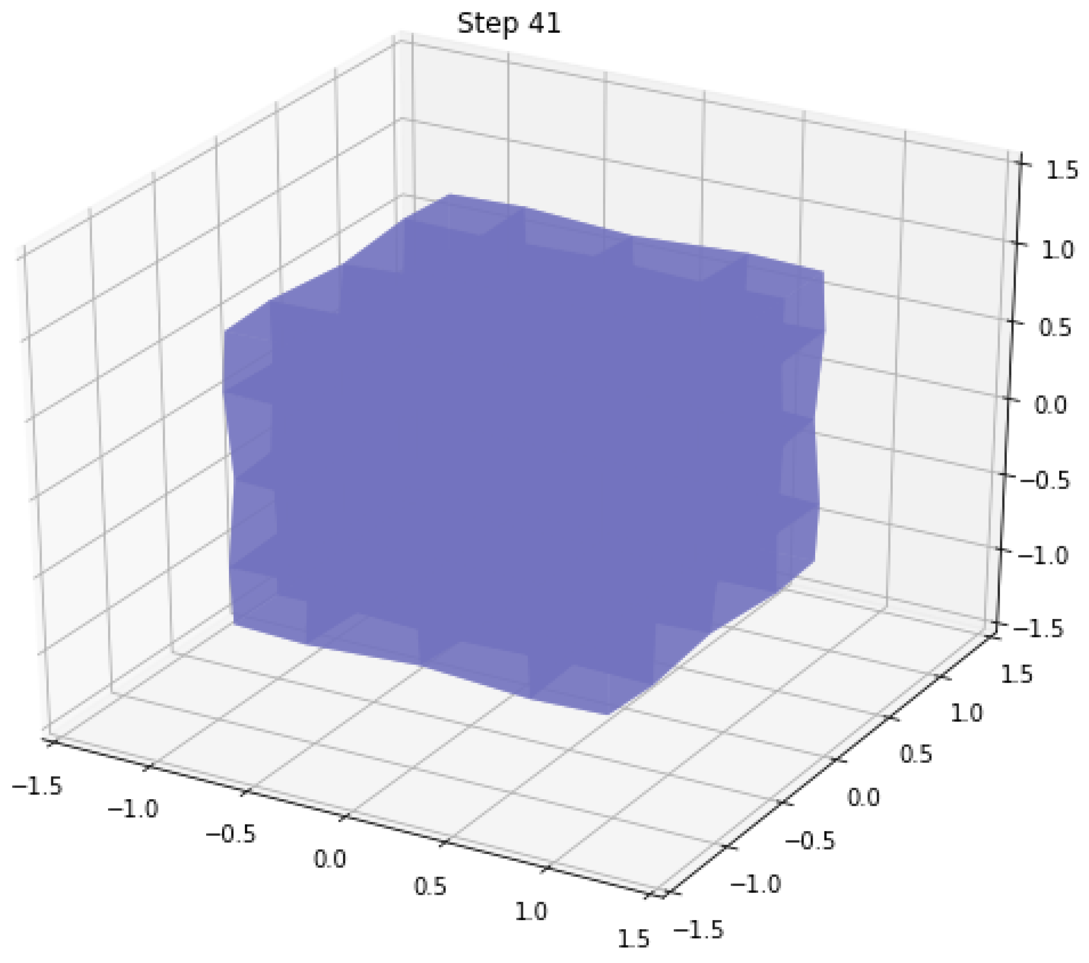
The 3D mesh was visualized using matplotlib’s 3D plotting capabilities. Figure 2 shows the initial sphere, and Figure 3 shows the mesh in the 41st step, with .

Figure 2.
Initial sphere.

Figure 3.
The 41st step.
The phenomenon of the cube gradually collapsing is caused by the finite element discretization of the nonlocal Monge–Ampère operator, where the implementation of the nonlocal operator is based on a Gaussian-weighted averaging scheme. This weighting approach causes the position update of each vertex to depend on the positions of its neighboring vertices. The weight calculation in the code indicates that vertices farther away have a smaller influence on the current vertex’s position. The update rule effectively moves each vertex toward the average position of its neighborhood, leading to a continuous aggregation of vertices toward the average position and, consequently, the collapse of the cube. The parameter controls the range of the nonlocal influence. A smaller value results in vertices being influenced only by very nearby vertices, whereas a larger value allows vertices to be influenced by more distant ones. If is not set appropriately, it may cause vertices to concentrate excessively at a certain position, leading to collapse. Nonlocal operators are used in physics and engineering to model systems with long-range interactions. Through this simple example, one can observe how nonlocal effects influence the overall behavior of a system. This phenomenon demonstrates potential stability issues in numerical simulations involving nonlocal models. In practical applications, careful selection of parameters (such as ) and numerical methods is necessary to ensure the stability of the system. From a geometric perspective, this collapsing behavior can be viewed as a simple geometric evolution process, akin to the mean curvature flow, in which a surface gradually moves in the direction of its mean curvature.
6. Discussion
While previous general studies have explored nonlocal parabolic Monge–Ampère operators, this paper zeroes in on the maximal regularity of parabolic Monge–Ampère operators, thereby facilitating the process to establish the existence of solutions. The paper reveals that the Monge–Ampère operator cannot exhibit compactness properties over the full domain without an exponential multiplier. To tackle this, we rely on the core concepts of maximal regularity existence. By making uniformly converge to 1 and bounding it at 1, we control the growth of nonlocal Monge–Ampère operators, ensuring maximal regularity. The author believes that this research methodology can be applied to other fractional operator studies.
Funding
This research was funded in part by the CAS AMSS-PolyU Joint Laboratory of Applied Mathematics and in part by the Natural Science Foundation in the U.S.
Data Availability Statement
The raw data supporting the conclusions of this article will be made available by the authors on request.
Acknowledgments
The author would like to express gratitude to the PhD supervisor and postdoctoral supervisor.
Conflicts of Interest
The author declares no conflicts of interest.
References
- Caffarelli, L.; Charro, F. On a fractional Monge-Ampère operator. Ann. PDE 2015, 4, 1–47. [Google Scholar] [CrossRef]
- Chen, W.; Li, Y.; Ma, P. The Fractional Laplacian; World Scientific Publishing Company: Singapore, 2019; pp. 1–344. [Google Scholar]
- Stein, E.M. Singular Integrals and Differentiability Properties of Functions; Princeton University Press: Princeton, NJ, USA, 1970; pp. 116–165. [Google Scholar]
- Caffarelli, L.; Silvestre, L. An extension problem related to the fractional Laplacian. Comm. Partial Differ. Equ. 2007, 32, 1245–1260. [Google Scholar] [CrossRef]
- Felmer, P.; Wang, L. Radial symmetry of positive solutions to equations involving the fractional Laplacian. Comm. Contemp. Math. 2014, 16, 1350023. [Google Scholar] [CrossRef]
- Musina, R.; Nazarov, A.I. On fractional Laplacians. Comm. Partial Differ. Equ. 2014, 39, 1780–1790. [Google Scholar] [CrossRef]
- Chen, W.; Fang, Y.; Yang, R. Liouville theorems involving the fractional Laplacian on a half space. Adv. Math. 2015, 274, 167–198. [Google Scholar] [CrossRef]
- Cabré, X.; Cinti, E. Sharp energy estimates for nonlinear fractional diffusion equations. Calc. Var. Partial Differ. Equ. 2014, 49, 233–269. [Google Scholar] [CrossRef]
- Cabré, X.; Sire, Y. Nonlinear equations for fractional Laplacians II: Existence, uniqueness, and qualitative properties of solutions. Trans. Am. Math. 2015, 367, 911–941. [Google Scholar] [CrossRef]
- Liu, X. The Radial Symmetry and Monotonicity of Solutions of Fractional Parabolic Equations in the Unit Ball. Symmetry 2025, 17, 781. [Google Scholar] [CrossRef]
- Chen, W.; Li, C.; Li, Y. A direct method of moving planes for the fractional Laplacian. Adv. Math. 2017, 308, 404–437. [Google Scholar] [CrossRef]
- Chen, W.; Li, C.; Li, G. Maximum principles for a fully nonlinear fractional order equation and symmetry of solutions. Calc. Var. Partial. Differ. Equ. 2017, 56, 29. [Google Scholar] [CrossRef]
- Chen, W.; Li, C. Maximum principles for the fractional p-Laplacian and symmetry of solutions. Adv. Math. 2018, 355, 735–758. [Google Scholar] [CrossRef]
- Berestycki, H.; Nirenberg, L. Monotonicity, symmetry and antisymmetry of solutions of semilinear elliptic equations. J. Geom. Phys. 1988, 5, 237–275. [Google Scholar] [CrossRef]
- Berestycki, H.; Nirenberg, L. Some qualitative properties of solutions of semilinear elliptic equations in cylindrical domains. In Analysis, et Cetera; Academic Press: Cambridge, MA, USA, 1990; pp. 115–164. [Google Scholar]
- Berestycki, H.; Nirenberg, L. On the method of moving planes and the sliding method. Bol. Soc. Bras. Mat. 1991, 22, 1–37. [Google Scholar] [CrossRef]
- Wu, L.; Chen, W. The sliding methods for the fractional p-Laplacian. Adv. Math. 2020, 361, 106933. [Google Scholar] [CrossRef]
- Chen, W.; Hu, Y. Monotonicity of positive solutions for nonlocal problems in unbounded domains. Funct. Anal. 2021, 281, 109187. [Google Scholar] [CrossRef]
- Liu, Z. Maximum principles and monotonicity of solutions for fractional p-equations in unbounded domains. J. Diff. Equ. 2021, 270, 1043–1078. [Google Scholar] [CrossRef]
- Ma, L.; Zhang, Z. Monotonicity of positive solutions for fractional p-systems in unbounded Lipschitz domains. Nonlinear Anal. 2020, 198, 111892. [Google Scholar] [CrossRef]
- Ma, L.; Zhang, Z. Monotonicity for fractional Laplacian systems in unbounded Lipschitz domains. Discret. Contin. Dyn. Syst. 2021, 41, 537–552. [Google Scholar] [CrossRef]
- Chen, W.; Hu, Y.; Ma, L. Moving planes and sliding methods for fractional elliptic and parabolic equations. Adv. Nonlinear Stud. 2023, 24, 359–398. [Google Scholar] [CrossRef]
- Dai, W.; Qin, G.; Wu, D. Direct Methods for pseudo-relativistic Schrödinger operators. J. Geom. Anal. 2021, 31, 5555–5618. [Google Scholar] [CrossRef]
- Le, P. Rigidity of phase transitions for the fractional elliptic Gross-Pitaevskii system. Fract. Calc. Appl. Anal. 2023, 26, 237–252. [Google Scholar] [CrossRef]
- Sun, M.; Liu, B. Sliding methods for a class of generalized fractional Laplacian equations. Bull. Malays. Math. Sci. Soc. 2022, 45, 2225–2247. [Google Scholar] [CrossRef]
- Qu, M.; Wu, J.; Zhang, T. Sliding method for the semi-linear elliptic equations involving the uniformly elliptic nonlocal operators. Discret. Contin. Dyn. Syst. 2021, 41, 2285–2300. [Google Scholar] [CrossRef]
- Chen, W.; Wu, L. Monotonicity and one-deimensional symmetry of solutions for fractional reaction-diffusion equations and various applications of sliding methods. Ann. Mat. 2024, 203, 173–204. [Google Scholar] [CrossRef]
- Du, G.; Wang, X. Monotonicity of solutions for parabolic equations involving nonlocal Monge-Ampère operator. Adv. Nonlinear Anal. 2024, 13, 47–150. [Google Scholar] [CrossRef]
- Fernandez-Real, X.; Ros-Oton, X. Regularity theory for general stable operators: Parabolic equations. J. Funct. Anal. 2017, 272, 4165–4221. [Google Scholar] [CrossRef]
- Liu, X. The Maximal Regularity of Nonlinear Second-Order Hyperbolic Boundary Differential Equations. Axioms 2024, 13, 884. [Google Scholar] [CrossRef]
- Chen, X.; Bao, G.; Li, G. The sliding method for the nonlocal Monge-Ampère operator. Nonlinear Anal. 2020, 196, 111786. [Google Scholar] [CrossRef]
- Gilboa, G.; Osher, S. Nonlocal operators with applications to image processing. Multiscale Model. Simul. 2008, 7, 1005–1028. [Google Scholar] [CrossRef]
- Aujol, J.F.; Aubert, G.; Blanc-Féraud, L.; Chambolle, A. Image decomposition into a bounded variation component and an oscillating component. J. Math. Imaging Vis. 2005, 22, 71–88. [Google Scholar] [CrossRef]
- Caffarelli, L.; Valdinoci, E. Nonlocal minimal surfaces. Commun. Pure Appl. Math. 2010, 63, 1111–1144. [Google Scholar] [CrossRef]
- Li, B.; Tang, R. Dynamic ritz projection of mean curvature flow and optimal L2 convergence of parametric FEM. SIAM J. Numer. Anal. 2025, in press. [Google Scholar]
Disclaimer/Publisher’s Note: The statements, opinions and data contained in all publications are solely those of the individual author(s) and contributor(s) and not of MDPI and/or the editor(s). MDPI and/or the editor(s) disclaim responsibility for any injury to people or property resulting from any ideas, methods, instructions or products referred to in the content. |
© 2025 by the author. Licensee MDPI, Basel, Switzerland. This article is an open access article distributed under the terms and conditions of the Creative Commons Attribution (CC BY) license (https://creativecommons.org/licenses/by/4.0/).