Reinforcing Moving Linear Model Approach: Theoretical Assessment of Parameter Estimation and Outlier Detection

Abstract

This paper reinforces the previously proposed moving linear (ML) model approach for time series analysis by introducing theoretically grounded enhancements. The ML model flexibly decomposes a time series into constrained and remaining components, enabling the extraction of trends and fluctuations with minimal structural assumptions. Building on this framework, we present two key improvements. First, we develop a theoretically justified evaluation criterion that facilitates coherent estimation of model parameters, particularly the width of the time interval. Second, we enhance the extended ML (EML) model by introducing a new outlier detection and estimation method that identifies both the number and locations of outliers by maximizing the reduction in AIC. Unlike the earlier version, the reinforced EML model simultaneously estimates outlier effects and improves model fit within a unified, likelihood-based framework. Empirical applications to economic time series illustrate the method’s superior ability to detect meaningful anomalies and produce stable, interpretable decompositions. These contributions offer a generalizable and theoretically supported approach to modeling nonstationary time series with structural disturbances.

1. Introduction

In [1], a moving linear (ML) model approach was proposed for decomposing time series data into two distinct components. Aimed specifically at business cycle analysis, this approach introduces a novel framework called the constrained-remaining components decomposition. In this framework, the time series is separated into two parts: the constrained component, governed by local linear model restrictions and primarily capturing the underlying trend, and the remaining component, subject to minimal constraints and reflecting cyclical movements, irregular fluctuations, and other disturbances in the data.

This separation under mild constraints represents a significant advancement in time series decomposition. While traditional methods typically focus on extracting basic patterns such as trends and cycles, the ML model approach provides a more flexible framework that can be applied across various fields. By employing simple model structures, the ML model achieves both broader applicability and effective handling of diverse data types and analytical objectives. Its ability to decompose time series into constrained and remaining components under flexible restrictions enhances its utility not only in economics but also in other disciplines dealing with temporal data.

A key parameter in the ML model approach is the width of the time interval (WTI), which governs the degree of local linearity captured by the constrained component. In ref. [1], the WTI is estimated using the maximum likelihood method within a state-space modeling framework, allowing the model to adapt efficiently to local variations in the time series. Accurate estimation of the WTI is essential for capturing both short-term fluctuations and long-term trends. In addition, ref. [2] introduced an intuitive, albeit somewhat ad hoc, measure called overall stability to evaluate the performance of the ML model approach, though this measure currently lacks a solid theoretical foundation.

In parallel with advances in decomposition techniques, anomaly detection has gained increasing attention in various fields, particularly in time series analysis (see, e.g., [3]). In business cycle research, identifying unexpected values or abrupt fluctuations is crucial, as these anomalies often correspond to major economic shocks such as policy changes, financial crises, or natural disasters. Numerous detection methods have been proposed (e.g., [4] and references therein), ranging from residual-based methods to machine learning techniques. However, many of these approaches are highly specialized and context-dependent. For example, ref. [5] evaluated three statistical outlier detection algorithms for water surface temperature data within an unsupervised learning framework. While such studies offer valuable insights, the proposed methods often lack general applicability and do not easily transfer to time series exhibiting nonstationarity or structural heterogeneity, such as those encountered in macroeconomic or financial domains.

In the context of ML modeling, ref. [6] proposed a two-step approach that combines time series decomposition with anomaly detection. While innovative, this method remains somewhat ad hoc and complex, lacking a unified theoretical foundation. Building upon this framework, ref. [7] introduced an extension known as the extended moving linear (EML) model, which incorporates a more systematic strategy for outlier detection and estimation. In the EML framework, outliers are treated as model parameters, with both their number and locations estimated simultaneously via the maximum likelihood method. Model selection is guided by the Akaike Information Criterion (AIC), and a heuristic yet effective procedure is implemented to enhance the search for outlier locations. This extension improves applicability to real-world economic data, where outliers, such as those resulting from pandemics or financial crises, can severely distort analysis if not appropriately addressed.

The ML model approach proposed by [1] and the EML model approach proposed by [7] have demonstrated strong capabilities in analyzing the mechanisms of business fluctuations (see [8]). Despite these advances, several challenges remain. First, the theoretical basis for WTI estimation and model evaluation is still underdeveloped. Second, although the EML framework incorporates outlier modeling, further refinement is needed in estimating and interpreting the effects of outliers, particularly their magnitude, persistence, and contribution to overall model fit. Specifically, it is essential to clarify the following: (i) the timing and location of each outlier; (ii) the magnitude of the perturbation associated with each outlier; (iii) whether their influence extends beyond the identified time point; (iv) how modeling each outlier affects the overall fit, as evaluated by the AIC.

The aim of this study is twofold. First, we seek to reinforce the theoretical foundation of the ML model approach, including WTI estimation and performance evaluation. Specifically, we provide a logically consistent discussion that supports the use of maximum likelihood estimation and propose a new criterion grounded in theory for evaluating model stability and suitability. Second, we refine the EML approach to outlier detection by introducing a new method based on maximizing the AIC reduction. This method quantifies each outlier’s contribution to model improvement and allows us to identify and model outliers more effectively and systematically. It also offers insight into whether and how each outlier should be modeled, imputed, or interpreted as a structural break.

Through these developments, we aim to provide a robust, generalizable framework for time series decomposition and outlier modeling. Our approach is particularly well suited for macroeconomic and financial applications, where data often include structural changes and unanticipated shocks. The state-space decomposition method proposed by [9] also serves as a useful point of reference throughout our analysis.

The remainder of this paper is organized as follows. Section 2 reviews the ML and EML model approaches. Section 3 presents theoretical developments and methodological refinements. Section 4 provides empirical illustrations that quantify outlier contributions and demonstrate the effectiveness of the proposed enhancements. Finally, Section 5 offers a summary and discussion.

2. A Review of the ML and EML Model Approaches

This section provides a comprehensive review of the ML model approach proposed by [1] and its extension, the EML model approach introduced by [7]. These approaches form the theoretical foundation for the methodology developed in this study.

2.1. The ML Model Approach

We begin by reviewing the ML model approach as presented in [1].

2.1.1. The Basic Model

We consider decomposing a time series $y_t$ into two unobserved components as follows:

$$y_t=s_t+f_t(t=1,2,\dots ,N),$$

(1)

where $s_t$ and $f_t$ denote the constrained and remaining components, respectively, t represents the time index, and N is the sample size. The constrained component $s_t$ captures long-term variation, such as trend, while the remaining component $f_t$ represents short-term fluctuation, including cyclical movement.

To ensure smoothness for the constrained component, we use a linear model of time t as follows:

$$s_t={\alpha }_n+{\beta }_{n}t,(t=n,n+1,\dots ,n+k-1).$$

(2)

Here, k is the width of the time interval (WTI), and ${\alpha }_n$ and ${\beta }_n$ are the coefficients in this interval. The n-th time interval is defined as $[n,n+k-1]$ for $n=1,2,\dots ,N-k+1$. A centered time variable within the n-th interval is introduced as

$$z_j=t-{\overline{t}}_n=j-{\displaystyle \frac{k+1}{2}}(j=1,2,\dots ,k),$$

where ${\overline{t}}_n=n+{\displaystyle \frac{k-1}{2}}$ is the midpoint of the time interval.

Substituting $t=z_j+{\overline{t}}_n$ into the model in Equation (2) we have

$$s_t={\mu }_n+{\beta }_n{z}_j(t=n+j-1;j=1,2,\dots ,k),$$

where ${\mu }_n={\alpha }_n+{\beta }_n{\overline{t}}_n$. The model in Equation (1) then becomes

$$y_t={\mu }_n+{\beta }_n{z}_j+f_t(t=n+j-1;j=1,2,\dots ,k),$$

(3)

which is referred to as the ML model.

2.1.2. State-Space Presentation of the ML Model

In the ML model given in Equation (3), the quantities ${\mu }_n$, ${\beta }_n$, and $\mathit{f}\left(n\right)$ are treated as parameters. To obtain stable estimates of these parameters, we adopt a Bayesian approach based on the following prior distributions.

Firstly, we assume that ${\mu }_n$ and ${\beta }_n$ vary smoothly with respect to n as

$${\mu }_n={\mu }_{n-1}+{\epsilon }_n,{\beta }_n={\beta }_{n-1}+{\varphi }_n,$$

(4)

by introducing diffuse priors for ${\epsilon }_n$ and ${\varphi }_n$. Specifically, we assume that ${\epsilon }_n\sim \mathcal{N}(0,{\eta }^2)$ and ${\varphi }_n\sim \mathcal{N}(0,{\eta }^2)$, where the variance ${\eta }^2$ is set to a sufficiently large value.

Then, to locally identify the remaining component $f_t$ uniquely, we introduce the following prior distributions for $f_1^{\left(n\right)}$ and $f_2^{\left(n\right)}$ as

$$f_1^{\left(n\right)}=-\sum _{j=1}^{k-1}{f}_j^{(n-1)}+e_{n+k-1},f_2^{\left(n\right)}=-\sum _{j=2}^k{\displaystyle \frac{z_{k-j}}{z_k}}{f}_j^{(n-1)}+e_{n+k-2},$$

(5)

which probabilistically maintain the orthogonality relationships between $f_t$ and ${\mu }_n$, as well as between $f_t$ and $z_j$ in the n-th time interval. Furthermore, to express the transition relationships, the priors for the other remaining component terms are given as follows:

$$f_j^{\left(n\right)}=f_{j-1}^{(n-1)}+e_{n+k-j}(j=3,4,\dots ,k).$$

(6)

In these equations, $e_{n+k-1},e_{n+k-2},\dots ,e_n$ represent a set of system noises, where it is assumed that $e_i\sim N(0,{\sigma }^2)$ i.i.d., with $n=1,2,\dots ,N-k+1$, and ${\sigma }^2$ is an unknown parameter.

Bayesian form of the ML model was constructed based on the above settings.

Moreover, under the settings

$$\begin{array}{ccc}& & {\mathit{x}}_n=\left[\begin{array}{c}{\mu }_n\\ {\beta }_n\\ f_1^{\left(n\right)}\\ f_2^{\left(n\right)}\\ ⋮\\ f_k^{\left(n\right)}\end{array}\right],\mathit{F}=\left[\begin{array}{cccccccc}1& 0& 0& \dots & \dots & \dots & \dots & 0\\ 0& 1& 0& \dots & \dots & \dots & \dots & 0\\ 0& 0& -1& -1& \dots & \dots & -1& 0\\ 0& 0& 0& -{\displaystyle \frac{z_{k-1}}{z_k}}& -{\displaystyle \frac{z_{k-2}}{z_k}}& \dots & \dots & -{\displaystyle \frac{z_1}{z_k}}\\ 0& 0& 0& 1& 0& \dots & \dots & 0\\ ⋮& ⋮& ⋮& 0& \ddots & \ddots & & ⋮\\ ⋮& ⋮& ⋮& ⋮& \ddots & \ddots & \ddots & ⋮\\ 0& 0& 0& 0& \dots & 0& 1& 0\end{array}\right],\hfill \end{array}$$

(7)

$$\begin{array}{ccc}& & {\mathit{v}}_n=\left[\begin{array}{c}{\epsilon }_n\\ {\varphi }_n\\ e_{n+k-1}\\ e_{n+k-2}\\ ⋮\\ e_n\end{array}\right],\mathit{y}\left(n\right)=\left[\begin{array}{c}{y}_{n+k-1}\\ y_{n+k-2}\\ ⋮\\ y_n\end{array}\right],\mathit{G}={\mathit{I}}_{k+2},\mathit{H}=\left[\begin{array}{ccc}{\mathbf{1}}_k& \mathit{z}& {\mathit{I}}_k\end{array}\right],\hfill \end{array}$$

(8)

a state-space representation for the moving linear model can be defined as

$${\mathit{x}}_n=\mathit{F}{\mathit{x}}_{n-1}+\mathit{G}{\mathit{v}}_n,$$

(9)

$$\mathit{y}\left(n\right)=\mathit{H}{\mathit{x}}_n$$

(10)

with ${\mathit{v}}_n\sim \mathrm{N}(\mathbf{0},\mathit{Q})$, where $\mathit{Q}=\mathrm{d}\mathrm{i}\mathrm{a}\mathrm{g}({\eta }^2,{\eta }^2,{\sigma }^2,\dots ,{\sigma }^2)$.

Therefore, given the initial conditions ${\mathit{x}}_{0|0}$ and ${\mathit{V}}_{0|0}$, and the observations $Y_{1:N}=\{y_1,y_2,\dots ,y_N\}$, we can compute the mean vectors and covariance matrices of the state variable ${\mathit{x}}_n$ for $n=1,2,\dots ,N-k+1$ using the Kalman filter and fixed-interval smoothing algorithms, as described below (for details, see [1,10]).

[Kalman filter]

$$\begin{array}{ccc}\hfill {\mathit{x}}_{n|n-1}& =& \mathit{F}{\mathit{x}}_{n-1|n-1},\hfill \\ \hfill {\mathit{V}}_{n|n-1}& =& \mathit{F}{\mathit{V}}_{n-1|n-1}{\mathit{F}}^{\mathtt{T}}+\mathit{G}\mathit{Q}{\mathit{G}}^{\mathtt{T}},\hfill \\ \hfill {\mathit{K}}_n& =& {\mathit{V}}_{n|n-1}{\mathit{H}}^{\mathtt{T}}{\left(\mathit{H}{\mathit{V}}_{n|n-1}{\mathit{H}}^{\mathtt{T}}\right)}^{-1},\hfill \\ \hfill {\mathit{x}}_{n|n}& =& {\mathit{x}}_{n|n-1}+{\mathit{K}}_n(\mathit{y}\left(n\right)-\mathit{H}{\mathit{x}}_{n|n-1}),\hfill \\ \hfill {\mathit{V}}_{n|n}& =& ({\mathit{I}}_{k+2}-{\mathit{K}}_n\mathit{H}){\mathit{V}}_{n|n-1}.\hfill \end{array}$$

[Fixed-interval smoothing]

$$\begin{array}{ccc}\hfill {\mathit{A}}_n& =& {\mathit{V}}_{n|n}{\mathit{F}}^{\mathtt{T}}{\mathit{V}}_{n+1|n}^{-1},\hfill \\ \hfill {\mathit{x}}_{n|N}& =& {\mathit{x}}_{n|n}+{\mathit{A}}_n({\mathit{x}}_{n+1|N}-{\mathit{x}}_{n+1|n}),\hfill \\ \hfill {\mathit{V}}_{n|N}& =& {\mathit{V}}_{n|n}+{\mathit{A}}_n({\mathit{V}}_{n+1|N}-{\mathit{V}}_{n+1|n}){\mathit{A}}_n^{\mathtt{T}}.\hfill \end{array}$$

Using the Kalman filter algorithm, component decomposition can be performed. In particular, by incorporating $f_t$ for $t=1,2,\dots ,N$ into the state vector ${\mathit{x}}_n$ for $n=1,2,\dots ,N-k+1$, the remaining component can be estimated within this model framework. The posterior distribution of the state vector ${\mathit{x}}_n$ obtained from fixed-interval smoothing is Gaussian, with mean ${\mathit{x}}_{n|N}$ and covariance matrix ${\mathit{V}}_{n|N}$. Accordingly, the estimate ${\widehat{f}}_t$ of $f_t$ can be extracted from ${\mathit{x}}_{n|N}$ for $n=1,2,\dots ,N-k+1$, and the estimate ${\widehat{s}}_t$ of the constrained component $s_t$ is obtained as ${\widehat{s}}_t=y_t-{\widehat{f}}_t$.

2.1.3. Method for Estimating the Parameters

In the setup described above, the WTI, k, and the variance, ${\sigma }^2$, of the system noise are the key parameters that characterize the ML model.

According to [9], based on the Kalman filter, the density function of the predictive distribution of $\mathit{y}\left(n\right)$ is expressed in the form of a normal distribution

$$f\left(\mathit{y}\left(n\right)\right|{\sigma }^2,k)={\displaystyle \frac{1}{\sqrt{{\left(2\pi \right)}^k\left|{\mathit{U}}_{n|n-1}\right|}}}exp\left(-{\displaystyle \frac{S^2\left(n\right)}{2}}\right)$$

with

$$S^2\left(n\right)={(\mathit{y}\left(n\right)-{\mathit{y}}_{n|n-1})}^{\mathtt{T}}{\mathit{U}}_{n|n-1}^{-1}(\mathit{y}\left(n\right)-{\mathit{y}}_{n|n-1}),$$

where ${\mathit{y}}_{n|n-1}$ and ${\mathit{U}}_{n|n-1}$ are the mean and covariance matrix of the predictive distribution of $\mathit{y}\left(n\right)$, given by

$${\mathit{y}}_{n|n-1}=\mathit{H}{\mathit{x}}_{n|n-1},{\mathit{U}}_{n|n-1}=\mathit{H}{\mathit{V}}_{n|n-1}{\mathit{H}}^{\mathtt{T}}.$$

Here, ${\mathit{x}}_{n|n-1}$ and ${\mathit{V}}_{n|n-1}$ are the mean and covariance matrix of the state ${\mathit{x}}_n$ in the prediction step of the Kalman filter.

To define the likelihood as the product of conditional probability distributions, it is necessary to structure the vectors and matrices related to the observation vector ${\mathit{y}}_n$ as follows. Specifically, $\mathit{y}\left(n\right)$, ${\mathit{y}}_{n|n-1}$, ${\mathit{V}}_{n|n-1}$, and $\mathit{H}$ are expressed as follows:

$$\begin{array}{ccc}& & \mathit{y}\left(n\right)=\left[\begin{array}{c}{y}_{n+k-1}\\ {\mathit{y}}^{\left(1\right)}\left(n\right)\end{array}\right],{\mathit{y}}_{n|n-1}=\left[\begin{array}{c}{\widehat{y}}_{n+k-1}\\ {\mathit{y}}_{n|n-1}^{\left(1\right)}\end{array}\right],\hfill \\ & & {\mathit{V}}_{n|n-1}=\left[\begin{array}{cc}a& {\mathit{b}}^{\mathtt{T}}\\ \mathit{b}& {\mathit{V}}_{n|n-1}^{\left(1\right)}\end{array}\right],\mathit{H}=\left[\begin{array}{cc}{\mathit{H}}_1& {\mathit{H}}_2\end{array}\right]\hfill \end{array}$$

with a being a scalar and $\mathit{b}$ a vector of appropriate dimension.

In this case, the density function of ${\mathit{y}}^{\left(1\right)}\left(n\right)$ is expressed as

$$f_1\left({\mathit{y}}^{\left(1\right)}\left(n\right)\right|{\sigma }^2,k)={\displaystyle \frac{1}{\sqrt{{\left(2\pi \right)}^{k-1}\left|{\mathit{U}}_{n|n-1}^{\left(1\right)}\right|}}}exp\left(-{\displaystyle \frac{S_1^2\left(n\right)}{2}}\right)$$

with

$$S_1^2\left(n\right)={({\mathit{y}}^{\left(1\right)}\left(n\right)-{\mathit{y}}_{n|n-1}^{\left(1\right)})}^{\mathtt{T}}{\left({\mathit{U}}_{n|n-1}^{\left(1\right)}\right)}^{-1}({\mathit{y}}^{\left(1\right)}\left(n\right)-{\mathit{y}}_{n|n-1}^{\left(1\right)}),$$

where

$${\mathit{U}}_{n|n-1}^{\left(1\right)}={\mathit{H}}_1{\mathit{V}}_{n|n-1}^{\left(1\right)}{\mathit{H}}_1^{\mathtt{T}}.$$

Thus, for $n=1$, the joint density function of $Y_{1:k}=\mathit{y}\left(1\right)$ is given by $f\left(\mathit{y}\left(1\right)\right|{\sigma }^2,k)$. For $n=2,3,\dots ,N-k+1$, the conditional density function of $y_{n+k-1}$ given ${\mathit{y}}^{\left(1\right)}\left(n\right)$ is expressed as

$$f_2\left(y_{n+k-1}\right|{\mathit{y}}^{\left(1\right)}\left(n\right),{\sigma }^2,k)={\displaystyle \frac{f\left(\mathit{y}\left(n\right)\right|{\sigma }^2,k)}{f_1\left({\mathit{y}}^{\left(1\right)}\left(n\right)\right|{\sigma }^2,k)}}(n=2,3,\dots ,N-k+1)$$

and the joint density function of $Y_{1:N}$ is expressed as follows:

$$L({\sigma }^2,k|Y_{1:N})=f\left(\mathit{y}\left(1\right)\right|{\sigma }^2,k)\prod _{n=2}^{N-k+1}{f}_2\left(y_{n+k-1}\right|{\mathit{y}}^{\left(1\right)}\left(n\right),{\sigma }^2,k).$$

When the observations for $Y_{1:N}$ are given, the function $L({\sigma }^2,k|Y_{1:N})$ becomes the likelihood function for ${\sigma }^2$ and k. Thus, the log-likelihood function is given by

$$\begin{array}{ccc}& & \mathrm{L}\mathrm{L}({\sigma }^2,k|Y_{1:N})=log\left(L({\sigma }^2,k|Y_{1:N})\right)=-{\displaystyle \frac{N}{2}}log\left(2\pi \right)-{\displaystyle \frac{1}{2}}\left(log|{\mathit{U}}_{1|0}|+S^2\left(1\right)\right)\hfill \\ & & -{\displaystyle \frac{1}{2}}\sum _{n=2}^{N-k+1}\left(log|{\mathit{U}}_{n|n-1}|-log|{\mathit{U}}_{n|n-1}^{\left(1\right)}|\right)-{\displaystyle \frac{1}{2}}\sum _{n=2}^{N-k+1}\left(S^2\left(n\right)-S_1^2\left(n\right)\right)\hfill \end{array}$$

(11)

Therefore, when k is given, the log-likelihood function $\mathrm{L}\mathrm{L}({\sigma }^2,k|Y_{1:N})$ defined in Equation (11) can be maximized to obtain the estimate ${\widehat{\sigma }}^2$ of ${\sigma }^2$. However, this optimization problem is difficult to solve analytically and generally requires numerical optimization methods.

Further, if ${\sigma }^2$ is temporarily set to 1 in the Kalman filter, the maximum likelihood estimate of ${\sigma }^2$ can be obtained analytically as

$${\widehat{\sigma }}^2={\displaystyle \frac{1}{N}}\left\{S^2\left(1\right)+\sum _{n=2}^{N-k+1}\left(S^2\left(n\right)-S_1^2\left(n\right)\right)\right\}.$$

Finally, the conditional log-likelihood function with respect to k, denoted as $\mathrm{L}\mathrm{L}({\widehat{\sigma }}^2,k\mid Y_{1:N})$, is a function of k alone. Therefore, the estimate of k can be obtained by maximizing $\mathrm{L}\mathrm{L}({\widehat{\sigma }}^2,k\mid Y_{1:N})$.

2.2. The EML Model Approach for Outlier Detection

Below, we provide another review of the EML model approach based on [7].

2.2.1. The Basic Model

Within the framework of the ML model approach, the following model is introduced to handle cases in which the time series $y_t$ contains outliers:

$$y_t=s_t+f_t+u_t(t=1,2,\dots ,N),$$

(12)

where $u_t$ represents the unusually varying component of the time series, which may include outliers. The other variables and associated assumptions in Equation (12) are consistent with those in Equation (1).

As a basic assumption, we suppose that the full dataset $Y_{1:N}=\{y_1,y_2,\dots ,y_N\}$ contains m outliers, denoted by $\{{\delta }_1,{\delta }_2,\dots ,{\delta }_m\}$, with $m\ll N$. If an outlier is present at time t, the corresponding unusually varying component $u_t$ is assigned one of the values from $\{{\delta }_1,{\delta }_2,\dots ,{\delta }_m\}$. If no outlier is present at time t, $u_t$ is set to zero. In other words, within the set $\{u_1,u_2,\dots ,u_N\}$, exactly m elements correspond one-to-one to the elements in the outlier set $\{{\delta }_1,{\delta }_2,\dots ,{\delta }_m\}$, while the remaining elements are zero.

Therefore, a simple setting for handling outliers can be employed (see [7]). Specifically, let $\mathsf{\delta }={({\delta }_1,{\delta }_2,\dots ,{\delta }_m)}^{\mathtt{T}}$ denote the vector of outliers. We consider $\{u_1,u_2,\dots ,u_N\}$ as a set of functions of the outliers $\mathsf{\delta }$, where each ${\delta }_i$ is treated as an unknown constant. By defining $y_t^{*}=y_t-u_t$, the transformed dataset $Y_{1:N}^{*}\left(\mathsf{\delta }\right)=\{y_1^{*},y_2^{*},\dots ,y_N^{*}\}$ becomes a version of the data with outliers removed. Applying $Y_{1:N}^{*}\left(\mathsf{\delta }\right)$ in place of $Y_{1:N}$ to the ML model approach, the log-likelihood $\mathrm{L}\mathrm{L}({\widehat{\sigma }}^2,k|Y_{1:N}^{*}\left(\mathsf{\delta }\right))$ defined in Equation (11) becomes a function of $\mathsf{\delta }$, enabling estimation via the maximum likelihood method.

While this setting is simple and intuitive, when m is large, it leads to high computational costs and may compromise the reliability of the estimation results.

2.2.2. Bayesian Approach to Outlier Estimation

To address the presence of multiple outliers in a more general framework, a Bayesian approach is introduced as follows.

In this framework, outliers are formally treated as time-varying random variables. Specifically, each outlier ${\delta }_j$ is represented as ${\delta }_{jn}$, and a transition equation is defined as

$${\delta }_{jn}={\delta }_{j(n-1)}(j=1,2,\dots ,m;n=1,2,\dots ,N),$$

which assumes that each outlier remains constant over time at step n.

By incorporating Equations (4)–(6), a Bayesian model is constructed for the EML model, with Equations (7) and (8) are redefined as follows:

$$\begin{array}{ccc}& & {\mathit{x}}_n=\left[\begin{array}{c}{\mu }_n\\ {\beta }_n\\ f_1^{\left(n\right)}\\ f_2^{\left(n\right)}\\ ⋮\\ f_k^{\left(n\right)}\\ {\delta }_{1n}\\ {\delta }_{2n}\\ ⋮\\ {\delta }_{mn}\end{array}\right],\mathit{F}=\left[\begin{array}{ccccccccc}1& 0& 0& \dots & \dots & \dots & \dots & 0& \\ 0& 1& 0& \dots & \dots & \dots & \dots & 0& \\ 0& 0& -1& -1& \dots & \dots & -1& 0& \\ 0& 0& 0& -{\displaystyle \frac{z_{k-1}}{z_k}}& -{\displaystyle \frac{z_{k-2}}{z_k}}& \dots & \dots & -{\displaystyle \frac{z_1}{z_k}}& \mathit{O}\\ 0& 0& 0& 1& 0& \dots & \dots & 0& \\ ⋮& ⋮& ⋮& 0& \ddots & \ddots & & ⋮& \\ ⋮& ⋮& ⋮& ⋮& \ddots & \ddots & \ddots & ⋮& \\ 0& 0& 0& 0& \dots & 0& 1& 0& \\ & & & & \mathit{O}& & & & {\mathit{I}}_m\end{array}\right],\hfill \\ & & \mathit{G}=\left[\begin{array}{c}{\mathit{I}}_{k+2}\\ \mathit{O}\end{array}\right],{\mathit{H}}_n=\left[\begin{array}{ccccccc}& & & {\psi }_{n+k-1}& & & \\ & & & & {\psi }_{n+k-2}& & \\ {\mathbf{1}}_k& \mathit{z}& {\mathit{I}}_k& & & \ddots & \\ & & & & & & \ddots \\ & & & & & & & {\psi }_n\end{array}\right],\hfill \end{array}$$

where ${\mathit{I}}_m$ denotes an m-dimensional identity matrix, $\mathit{O}$ denotes a zero matrix with appropriate dimensions, and ${\psi }_i$ is a concatenation function defined such that ${\psi }_i=1$ if $u_i={\delta }_j$ for $j\in \{1,2,\dots ,m\}$, and ${\psi }_i=0$ otherwise, for $i=n+k-1,n+k-2,\dots ,n$.

Then, under the setting $\mathit{H}={\mathit{H}}_n$, the state space presentation for the Bayesian EML model can be expressed using Equations (9) and (10).

Based on the above formulation and by applying $\mathit{H}={\mathit{H}}_n$ in both the Kalman filter and fixed-interval smoothing algorithms, estimates of the state vector can be obtained. Consequently, the estimates $\widehat{\mathsf{\delta }}$ for the outliers, as well as the estimates of the remaining components, can be extracted from ${\mathit{x}}_{n|N}$ for $n=1,2,\dots ,N-k+1$. Specifically, $\widehat{\mathsf{\delta }}$ corresponds to the elements from the $(k+3)$-th to the $(k+2+m)$-th entries in the vector ${\mathit{x}}_{N-k+1|N}$, which depend only on the smoothing result at $n=N-k+1$. The corresponding variances of the outlier estimates are given by the diagonal elements of the covariance matrix ${\mathit{V}}_{N-k+1|N}$ from the $(k+3)$-th to the $(k+2+m)$-th rows.

2.2.3. Outlier Detection and Estimation

The key steps for identifying the locations of outliers and estimating their values are as follows. First, ignoring the presence of outliers, the time series is decomposed into the constrained and remaining components using the ML model approach. The initial outlier locations are then set as the time points corresponding to the top m values of the remaining component in terms of their squared magnitudes.

Next, the EML model provides Bayesian-type estimates of the outliers, which approximate maximum likelihood estimates. These estimates enable the computation of an approximate maximum log-likelihood, which in turn allows the number of outliers to be determined using the minimum AIC criterion.

Subsequently, the estimated values of the outliers are normalized by their standard deviations. By ranking the normalized squared estimates, a new set of outlier locations is obtained. This update distinguishes the revised locations from the initial setting and enables more accurate estimation based on the updated locations. The procedure for updating outlier locations is repeated iteratively until the estimation results converge.

Although the final step is well-structured, it remains somewhat ad hoc, and its performance in detecting outliers is unstable due to the lack of consideration for interrelationships among outliers. Revising this step is a central objective of the present study.

3. New Development to Reinforce Previous Findings

3.1. The Aims

In the current ML model approach, the WTI is estimated using the maximum likelihood method. From the perspective of statistical analysis, the use of maximum likelihood itself poses no particular issues. However, as maximum likelihood estimation is inherently model-dependent, our aim is not merely to justify its application but to provide theoretical support for both the model and the estimation method through logical and systematic discussion. In particular, we seek to develop a theoretical understanding of the critical role that WTI plays in improving the model’s overall performance.

Although WTI was originally introduced as a practical device, we endeavor to clarify, from a theoretical standpoint, how it facilitates the effective separation of constrained and remaining components and contributes to the stabilization of subsequent estimation procedures. This theoretical elaboration is essential for reinforcing the model’s interpretability and robustness.

In addition, when comparing different estimation methods, likelihood values are not always a reliable basis due to fundamental differences in model structure. To address this issue, another key objective is to propose new evaluation metrics based on the variance–covariance structures of the decomposed components. These metrics are intended to enable a more holistic assessment of the decomposition results and thereby enhance the credibility of the ML model approach. Unlike existing methods that rely narrowly on likelihood, the proposed metrics capture a wider range of estimation characteristics and offer a theoretically sound and practically useful basis for model comparison and evaluation.

Furthermore, as noted in Section 2.2.3, while the existing EML approach for identifying outlier locations is well-designed, it remains somewhat ad hoc and can exhibit unstable performance due to its neglect of the interrelationships among outliers. To address these limitations, we propose a method based on the maximization of AIC reduction, which identifies outliers by evaluating their individual contributions to the decrease in the AIC. This approach selects outlier locations that most significantly enhance model fit. By introducing this theoretically grounded and computationally efficient method, the outlier detection process becomes more stable, systematic, and reliable.

Collectively, these enhancements, which clarify the theoretical role of the ML approach, propose additional evaluation metrics, and refine the outlier detection process, represent significant steps toward completing and strengthening the ML and EML model approaches as a coherent and reliable framework for time series analysis.

3.2. Reinforcing the ML Model Approach

In this section, we aim to reinforce the ML model approach by offering theoretical insights into the evaluation of results by proposing additional evaluation metrics.

3.2.1. Variance-Preserving Adjustment of the Decomposed Components

Within the context of the ML model approach, the constrained-remaining components decomposition yields ${\widehat{s}}_t$ and ${\widehat{f}}_t$ as the decomposed constrained and remaining components, respectively, such that the original time series $y_t$ can be represented as

$$y_t={\widehat{s}}_t+{\widehat{f}}_t(t=1,2,\dots ,N).$$

(13)

Obviously, the component decomposition in Equation (13) is average-invariant, ensuring that the equality $\overline{y}=\overline{s}+\overline{f}$ holds, where

$$\overline{y}={\displaystyle \frac{1}{N}}\sum _{t=1}^N{y}_t$$

denotes the average of the time series $y_t$, and $\overline{s}$ and $\overline{f}$ denote the averages of the constrained and remaining components, respectively. Note that in the ML model approach, the remaining component is adjusted so that $\overline{f}$ becomes zero. As a result, $\overline{s}$ is equal to $\overline{y}$. This implies that the average level of the constrained component matches that of the original time series.

In addition to the average invariance of the component decomposition in Equation (13), variance–invariance is also desirable; however, it cannot be consistently maintained by the ML model approach. Let $\mathrm{V}\mathrm{a}\mathrm{r}\left(y_t\right)$ denote the sample variance of $y_t$, while $\mathrm{V}\mathrm{a}\mathrm{r}\left(s_t\right)$ and $\mathrm{V}\mathrm{a}\mathrm{r}\left(f_t\right)$ denote the sample variances of ${\widehat{s}}_t$ and ${\widehat{f}}_t$, respectively, and let $\mathrm{C}\mathrm{o}\mathrm{v}(s_t,f_t)$ denote their sample covariance. Then, the following relationship holds:

$$\mathrm{V}\mathrm{a}\mathrm{r}\left(y_t\right)=\mathrm{V}\mathrm{a}\mathrm{r}\left(s_t\right)+\mathrm{V}\mathrm{a}\mathrm{r}\left(f_t\right)+2\mathrm{C}\mathrm{o}\mathrm{v}(s_t,f_t).$$

If $\mathrm{C}\mathrm{o}\mathrm{v}(s_t,f_t)=0$, indicating no correlation between the decomposed components, then we have

$$\mathrm{V}\mathrm{a}\mathrm{r}\left(y_t\right)=\mathrm{V}\mathrm{a}\mathrm{r}\left(s_t\right)+\mathrm{V}\mathrm{a}\mathrm{r}\left(f_t\right).$$

(14)

Thus, the component decomposition becomes variance-invariant, meaning that the variance of the original time series equals the sum of the variances of the decomposed components without any covariance term.

In the ML model approach, the decomposed components are generally uncorrelated due to the model specification. However, this property may vary depending on the parameter settings and the characteristics of the data. When a correlation exists between the components, an adjustment can be made to restore variance–invariance by introducing the following regression model:

$${\widehat{f}}_t=\gamma ({\widehat{s}}_t-\overline{y})+{\epsilon }_t(t=1,2,\dots ,N),$$

(15)

where ${\widehat{s}}_t-\overline{y}$ is the centered constrained component, $\gamma$ is the regression coefficient, and ${\epsilon }_t$ is the residual term.

Based on the least squares estimate $\widehat{\gamma }$ of $\gamma$, the remaining component can be adjusted as follows:

$${\tilde{f}}_t={\widehat{\epsilon }}_t={\widehat{f}}_t-\widehat{\gamma }({\widehat{s}}_t-\overline{y}),$$

(16)

where ${\tilde{f}}_t$ represents the adjusted remaining component, which can be used as the final decomposed result.

By the orthogonality property of least squares estimation, ${\tilde{f}}_t$ is uncorrelated with ${\widehat{s}}_t$, thereby ensuring that variance–invariance is preserved when ${\tilde{f}}_t$ is used as the final decomposed result in place of ${\widehat{f}}_t$. This adjustment, which renders the decomposed components uncorrelated, is referred to as a variance-preserving adjustment.

Incidentally, as shown in Equations (15) and (16), the variance-preserving adjustment effectively eliminates the portion of the remaining component that is correlated with the constrained component while maintaining the smoothness of the latter. Although an alternative method of achieving variance preservation—namely, adjusting the constrained component based on the remaining component—is theoretically possible, it is not recommended because it may compromise the smoothness of the trend.

Through the variance-preserving adjustment, the ML model approach can maintain the invariance properties of the constrained-remaining components decomposition—namely, both average invariance and variance–invariance. In statistical analysis, the information contained in a dataset is primarily conveyed through its variance; therefore, ensuring variance–invariance guarantees the preservation of informational content before and after component decomposition.

3.2.2. Structural Examination of Variances for the Decomposed Components

As discussed in the previous section, the variance-preserving adjustment ensures that the constrained-remaining components decomposition maintains the variance-invariant property, as shown in Equation (14). As a result, for a given time series $y_t$, the total variance of the two decomposed components remains constant, as expressed by the following equation:

$$\mathrm{V}\mathrm{a}\mathrm{r}\left(s_t\right)+\mathrm{V}\mathrm{a}\mathrm{r}\left(f_t\right)=\mathrm{V}\mathrm{a}\mathrm{r}\left(y_t\right)=\mathrm{c}\mathrm{o}\mathrm{n}\mathrm{s}\mathrm{t}\mathrm{.}$$

(17)

To further investigate the relationship between the decomposed components, define the product of their variances as

$$\mathrm{P}\mathrm{V}=\mathrm{V}\mathrm{a}\mathrm{r}\left(s_t\right)\mathrm{V}\mathrm{a}\mathrm{r}\left(f_t\right).$$

It can be confirmed that PV reaches its maximum when the variances of the decomposed components are equal, that is, when $\mathrm{V}\mathrm{a}\mathrm{r}\left(s_t\right)=\mathrm{V}\mathrm{a}\mathrm{r}\left(f_t\right)$. In this case, by also referring to Equation (17), it becomes clear that $\mathrm{V}\mathrm{a}\mathrm{r}\left(s_t\right)=\mathrm{V}\mathrm{a}\mathrm{r}\left(f_t\right)=0.5\mathrm{V}\mathrm{a}\mathrm{r}\left(y_t\right)$, and the maximum value of PV is given by $0.25{\left(\mathrm{V}\mathrm{a}\mathrm{r}\left(y\right)\right)}^2$.

On the other hand, when the WTI, k, is small, the constrained component ${\widehat{s}}_t$ absorbs a large part of the fluctuations of the time series, exhibiting large variability. As a result, the remaining component ${\widehat{f}}_t$ contains relatively small fluctuations, leading to

$$\mathrm{V}\mathrm{a}\mathrm{r}\left(s_t\right)>\mathrm{V}\mathrm{a}\mathrm{r}\left(f_t\right).$$

As k increases, $\mathrm{V}\mathrm{a}\mathrm{r}\left(s_t\right)$ decreases and $\mathrm{V}\mathrm{a}\mathrm{r}\left({\widehat{f}}_t\right)$ increases, so that $\mathrm{V}\mathrm{a}\mathrm{r}\left(s_t\right)-\mathrm{V}\mathrm{a}\mathrm{r}\left(f_t\right)$ gradually becomes smaller. Thus, the product of variances, PV, behaves as a monotonically non-decreasing function with respect to k.

When k continues to increase, $\mathrm{V}\mathrm{a}\mathrm{r}\left(s_t\right)$ and $\mathrm{V}\mathrm{a}\mathrm{r}\left(f_t\right)$ eventually become equal so that PV reaches its maximum value. Beyond this point, as k increases further, PV becomes a monotonically non-increasing function of k.

When attempting to extract information related to business cycle fluctuations from time series data, such information is often captured by the variations in the remaining component. Therefore, it is natural to expect that the variance of the remaining component will be relatively large in this context. Based on this expectation, one may consider increasing the value of the parameter k—especially when starting from a small value—in order to achieve a higher PV and thereby better capture cyclical variations.

Simply increasing k to maximize PV, without due consideration of these structural constraints, may result in a decomposition that violates the fundamental assumptions of the model.

In summary, the absolute value of PV cannot be directly used as a criterion for evaluating the quality of a decomposition. Nevertheless, PV serves as an important indicator of the relationship between the characteristics of the time series data and the parameter k. Therefore, for a given dataset, it is more meaningful to examine how PV varies with k rather than focusing on its absolute magnitude.

3.2.3. Assessing the Structural Changes in Decomposed Components

While the previously introduced indicator PV captures the relative changes in the variances of the two components as the parameter k varies, it does not reflect the internal stability or continuity of each component across successive values of k. In other words, PV illustrates how the variances of the constrained and remaining components, $\mathrm{V}\mathrm{a}\mathrm{r}\left(s_t\right)$ and $\mathrm{V}\mathrm{a}\mathrm{r}\left(f_t\right)$, change in relation to each other, but it does not indicate whether the structural changes within each decomposed component occur gradually or abruptly as k increases.

To address this limitation, we consider an alternative approach that evaluates the similarity of each component’s decomposed results with respect to a unit change in the successive value of k. This similarity can be quantified using the covariance between the decomposed results at two consecutive settings.

Specifically, for the constrained component, let ${\widehat{s}}_t(k-1)$ and ${\widehat{s}}_t\left(k\right)$ denote the decomposed results obtained at $k-1$ and k, respectively. Instead of using the variance $\mathrm{V}\mathrm{a}\mathrm{r}\left(s_t\right)$, we introduce the covariance $\mathrm{C}\mathrm{o}\mathrm{v}(s_t(k-1),s_t\left(k\right))$ between ${\widehat{s}}_t(k-1)$ and ${\widehat{s}}_t\left(k\right)$ as an alternative indicator. If the decomposed results change only slightly with respect to k, then the covariance $\mathrm{C}\mathrm{o}\mathrm{v}(s_t(k-1),s_t\left(k\right))$ will be close to $\mathrm{V}\mathrm{a}\mathrm{r}\left(s_t\right)$, suggesting that the component ${\widehat{s}}_t$ remains stable as k increases.

A similar argument applies to the remaining component. Instead of using the variance $\mathrm{V}\mathrm{a}\mathrm{r}\left(f_t\right)$, we use the covariance $\mathrm{C}\mathrm{o}\mathrm{v}(f_t(k-1),f_t\left(k\right))$ between ${\widehat{f}}_t(k-1)$ and ${\widehat{f}}_t\left(k\right)$, which denote the decomposed remaining components obtained at $k-1$ and k, respectively.

Building upon this idea, we propose an extended measure analogous to PV that incorporates both the relative changes in variance between the two components and the degree of continuity within each component across successive values of k. Specifically, sharing similar properties with $\mathrm{P}\mathrm{V}$, we introduce the product of covariances (PCV) for decomposed components as follows:

$$\mathrm{P}\mathrm{C}\mathrm{V}\left(k\right)=\mathrm{C}\mathrm{o}\mathrm{v}(s_t(k-1),s_t\left(k\right))·\mathrm{C}\mathrm{o}\mathrm{v}(f_t(k-1),f_t\left(k\right)),$$

which is defined as a function of k and serves as an indicator that is more sensitive to variability. $\mathrm{P}\mathrm{C}\mathrm{V}\left(k\right)$ simultaneously captures both the inter-component variance relationship and the intra-component continuity with respect to k. It provides a more comprehensive understanding of the decomposition behavior, particularly in applications where both smooth transitions and balanced variance allocation are critical considerations.

The above concepts serve as useful foundations for constructing indicators to evaluate decomposition results. From this perspective, a set of decomposed results obtained at a value of k that induces smaller fluctuations in the indicator can be regarded as reflecting a more stable underlying structure. Accordingly, it is preferable to adopt the decomposition corresponding to such a value of k, as it is likely to provide a more reliable representation of the time series structure. Furthermore, similar indicators can be developed to facilitate comparisons with alternative decomposition methods.

3.2.4. Evaluation Metrics for Assessing Decomposition Stability

In the constrained-remaining components decomposition, evaluating the stability of the results is essential for understanding the underlying structure of a time series. One type of indicator for such evaluation is $\mathrm{P}\mathrm{C}\mathrm{V}\left(k\right)$. Since this indicator varies with the parameter k, it potentially reflects the structure of the decomposed results. However, it may exhibit unstable behavior depending on the characteristics of the time series and the chosen decomposition framework. This section discusses a more robust evaluation strategy based on $\mathrm{P}\mathrm{C}\mathrm{V}\left(k\right)$ and explores its relationship to both likelihood-based estimation and alternative decomposition methods.

Therefore, by normalizing $\mathrm{P}\mathrm{C}\mathrm{V}\left(k\right)$, we define the serial index of structural similarity (SISS) as follows:

$$\mathrm{S}\mathrm{I}\mathrm{S}\mathrm{S}\left(k\right)={\displaystyle \frac{2\sqrt{\left|\mathrm{P}\mathrm{C}\mathrm{V}\right(k\left)\right|}}{\mathrm{V}\mathrm{a}\mathrm{r}\left(y_t\right)}}={\displaystyle \frac{2\sqrt{|\mathrm{C}\mathrm{o}\mathrm{v}(s_t(k-1),s_t\left(k\right))·\mathrm{C}\mathrm{o}\mathrm{v}(f_t(k-1),f_t\left(k\right))|}}{\mathrm{V}\mathrm{a}\mathrm{r}\left(y_t\right)}}.$$

(18)

In Equation (18), a dimensional adjustment is made to account for the fact that the maximum value of $\mathrm{P}\mathrm{C}\mathrm{V}\left(k\right)$ can approach $0.25{\left(\mathrm{V}\mathrm{a}\mathrm{r}\left(y_t\right)\right)}^2$, which allows $\mathrm{S}\mathrm{I}\mathrm{S}\mathrm{S}\left(k\right)$ to potentially reach a value close to 1. SISS serves as a metric for evaluating the overall structural similarity of the decomposition results across successive values of k. A smaller value of SISS indicates a significant structural change in the decomposition due to a shift in k. Note that the use of the absolute value inside the square root is not theoretically essential; it is included as a safeguard against the possibility of negative covariance values.

Furthermore, for a given value of k, the similarity between the decomposed results—namely, $s_t^{*}$ and $f_t^{*}$—obtained by another method (used as a comparison counterpart) and those from the ML model approach can be evaluated by replacing $s_t(k-1)$ and $f_t(k-1)$ in the SISS formula in Equation (18) with $s_t^{*}$ and $f_t^{*}$, respectively. We refer to this variant of SISS as the mutual index of structural similarity (MISS). A higher MISS value indicates that the results obtained by the comparison method closely resemble those derived from the ML model approach.

However, $\mathrm{S}\mathrm{I}\mathrm{S}\mathrm{S}\left(k\right)$ may exhibit unstable behavior depending on the characteristics of the time series. To address this, we define an index of instability (IOI) based on $\mathrm{S}\mathrm{I}\mathrm{S}\mathrm{S}\left(k\right)$ as follows:

$$\mathrm{I}\mathrm{O}\mathrm{I}\left(k\right)=\Delta log\mathrm{S}\mathrm{I}\mathrm{S}\mathrm{S}\left(k\right)=log\mathrm{S}\mathrm{I}\mathrm{S}\mathrm{S}\left(k\right)-log\mathrm{S}\mathrm{I}\mathrm{S}\mathrm{S}(k-1).$$

(19)

As shown in Equation (19), $\mathrm{I}\mathrm{O}\mathrm{I}\left(k\right)$ is defined as the difference in the logarithm of $\mathrm{S}\mathrm{I}\mathrm{S}\mathrm{S}\left(k\right)$ with respect to k and thus serves as a measure of the relative rate of change of $\mathrm{S}\mathrm{I}\mathrm{S}\mathrm{S}\left(k\right)$. A small value of $\mathrm{I}\mathrm{O}\mathrm{I}\left(k\right)$ indicates that $\mathrm{S}\mathrm{I}\mathrm{S}\mathrm{S}\left(k\right)$ changes gradually as k increases, suggesting that the decomposition structure remains relatively stable with respect to k. Accordingly, a value of k associated with a small magnitude of $\mathrm{I}\mathrm{O}\mathrm{I}\left(k\right)$ can be considered a structurally stable decomposition point. Thus, $\mathrm{I}\mathrm{O}\mathrm{I}\left(k\right)$ may be used, alongside the likelihood, as a reference indicator for selecting an appropriate value of k and evaluating the estimation method.

3.2.5. Bidirectional Processing and Recursive Decomposition Strategies

The original ML model approach is processed in the order of $n=1,2,\dots ,N-k+1$, and the component decomposition is conducted according to this order. This is referred to as forward processing. On the other hand, it is referred to as backward processing if the same model is configured with the component decomposition proceeding in reverse order, that is, $n=N-k+1,N-k,\dots ,1$. Since the correspondence between decomposed results and observations differs between the forward and backward processings, the results of component decomposition may also differ.

By averaging the estimation results at the same time point obtained from these two processings, a more stable and accurate component decomposition can be achieved. In other words, integrating the results obtained through bidirectional estimation—namely, the forward and backward processings—can provide more reliable and robust outcomes compared to estimation based solely on forward processing.

It should be noted that the constrained-remaining components decomposition is not necessarily completed in a single step. If necessary, the ML model approach can be repeatedly applied to the resulting components to further divide a given component into two or more subcomponents. However, the interpretation and use of such decomposition results should be carefully considered in light of the characteristics of the data being analyzed, as well as the application’s objectives and context.

Moreover, ref. [1] proposed an orthogonalization method for transforming multiple resulting components into mutually uncorrelated time series.

3.3. Reinforcing the EML Model Approach

In this section, we aim to reinforce the EML model approach to improve the methodology for identifying the locations of outliers and estimating their values.

The original problem concerns identifying and estimating m outliers in a dataset of size N, where m is assumed to be much smaller than N. This task poses a combinatorial challenge and is therefore regarded as a nontrivial endeavor. To tackle this issue effectively, it is essential to first obtain some indications of potential outlier locations.

For completeness, the full procedure developed in this study is presented below. Among the steps, the third and fourth represent novel contributions of this work.

3.3.1. Determining the Potential Locations of Outliers

When a constrained-remaining components decomposition is performed using the ML model approach with a large WTI, most outliers tend to be absorbed into the estimate of the remaining component. Therefore, a provisional estimate ${\tilde{f}}_t$ of the remaining component can serve as a useful reference. Specifically, we may assume that

$${\tilde{f}}_t\approx f_t+u_t(t=1,2,\dots ,N).$$

Let ${\widehat{f}}_t$ represent a realized estimate from the random process ${\tilde{F}}_t$, and let $f_t$ be a sample drawn from a random process $F_t$, where ${\tilde{F}}_t=F_t+u_t$, and $u_t$ is assumed to possibly contain a potential outlier. It is further assumed that $E\left\{F_t\right\}=0$ and $E\left\{F_t^2\right\}=C>0$. The expected value $E\left\{{\tilde{F}}_t^2\right\}$ can be expressed as follows:

$$E\left\{{\tilde{F}}_t^2\right\}=E\{F_t^2+2F_t{u}_t+u_t^2\}.$$

Thus, we have

$$E\left\{{\tilde{F}}_t^2\right\}=\left\{\begin{array}{cc}C+{\delta }_j^2\hfill & \mathrm{if}{u}_t\mathrm{contains}\mathrm{an}\mathrm{outlier},\mathrm{say},{\delta }_j\mathrm{for}1\le j\le m\hfill \\ C\hfill & \mathrm{otherwise}\hfill \end{array}\right..$$

This indicates that $E\left\{{\tilde{F}}_t^2\right\}$ becomes particularly large when $u_t$ potentially contains an outlier. Additionally, when $u_t=0$, ${\tilde{f}}_t^2$ provides an unbiased estimate of ${\tilde{F}}_t^2=F_t^2$.

In summary, a large value of ${\tilde{f}}_t^2$ is likely to reflect the presence of ${\delta }_t^2$. When the upper limit for the number of potential outliers is set to M, and the top M squared terms of the remaining component satisfy ${\tilde{f}}_{t_1}^2\ge {\tilde{f}}_{t_2}^2\ge \dots \ge {\tilde{f}}_{t_M}^2$, it is reasonable to infer that ${\tilde{f}}_{t_1}$ corresponds to the largest outlier in amplitude, ${\tilde{f}}_{t_2}$ to the second largest, and so on. In other words, the order in which potential outlier locations are examined can be established as

$$t_1,t_2,\dots ,t_M.$$

(20)

Subsequently, the potential outlier locations can be estimated in this order.

3.3.2. Estimating Outliers

Assume that, for a given integer M, a vector of potential outliers $\mathsf{\delta }={({\delta }_1,{\delta }_2,\dots ,{\delta }_M)}^{\mathtt{T}}$ is specified, and that a subvector ${\mathsf{\delta }}^{\left(m\right)}$ consisting of m elements selected from $\mathsf{\delta }$ is incorporated into the model for $m=1,2,\dots ,M$. When the locations of outliers are determined (even if only tentatively), applying the EML model approach yields a Bayesian-type estimate ${\widehat{\mathsf{\delta }}}^{\left(m\right)}$ for the outliers (see [7]). This estimate corresponds to the maximum a posteriori (MAP) estimate and closely approximates the maximum likelihood estimate. Therefore, the estimates ${\widehat{\mathsf{\delta }}}^{\left(m\right)}$ can be substituted into ${\mathsf{\delta }}^{\left(m\right)}$ in $Y_{1:N}^{*}\left({\mathsf{\delta }}^{\left(m\right)}\right)$ to obtain an approximation of the maximum likelihood, $\mathrm{L}\mathrm{L}({\widehat{\sigma }}^2,k|Y_{1:N}^{*}\left({\widehat{\mathsf{\delta }}}^{\left(m\right)}\right))$, which is defined in Equation (11).

This allows for an approximate calculation of the corresponding AIC, defined by

$$\mathrm{A}\mathrm{I}\mathrm{C}\left(m\right)=-2\mathrm{L}\mathrm{L}({\widehat{\sigma }}^2,k|Y_{1:N}^{*}\left({\widehat{\mathsf{\delta }}}^{\left(j\right)}\right))+2(m+1),$$

(21)

which depends on the value of m. Thus, the number m of outliers can be determined using the minimum AIC method (see [11]).

3.3.3. Updating the Locations and Determining the Number of Outliers

The aforementioned method for determining the potential locations of outliers is simple but does not account for the uncertainty associated with the estimated values of the outliers. To address this limitation, ref. [7] proposes a method for updating the locations of outliers using standardized estimates—specifically, the estimates of outliers normalized by dividing them by their standard deviations. However, this approach still does not consider the interdependence among outliers, and challenges remain in accurately estimating their locations.

Here, we propose a new approach that simultaneously determines the locations and the number of outliers by taking into account their interdependence, with the aim of maximizing the reduction in AIC. This approach is referred to as the AIC reduction maximization method.

Firstly, given the sequential set of potential outlier locations $\{t_1,t_2,\dots ,t_m\}$, we estimate the model parameters for each number of outliers $m=0,1,\dots ,M$, and compute the corresponding values of $\mathrm{A}\mathrm{I}\mathrm{C}\left(m\right)$ using Equation (21). Specifically, the case of $m=0$ assumes no outliers are present; $m=1$ assumes a single outlier at time $t_1$; $m=2$ assumes outliers at times $t_1$ and $t_2$; and so forth. In this manner, we obtain the sequence of AIC values as

$$\left\{\mathrm{A}\mathrm{I}\mathrm{C}\right(m);m=0,1,\dots ,M\}.$$

(22)

Furthermore, based on the sequence of AIC values given in Equation (22), a corresponding sequence of AIC differences is generated as

$$\mathrm{D}\mathrm{A}\mathrm{I}\mathrm{C}\left(m\right),m=1,2,\dots ,M,$$

(23)

where $\mathrm{D}\mathrm{A}\mathrm{I}\mathrm{C}\left(m\right)=\mathrm{A}\mathrm{I}\mathrm{C}\left(m\right)-\mathrm{A}\mathrm{I}\mathrm{C}(m-1)$. In the DAIC sequence shown in Equation (23), any integer i for which $\mathrm{D}\mathrm{A}\mathrm{I}\mathrm{C}\left(i\right)<0$ can be interpreted as indicating that the outlier located at time point $t_i$ is of particular importance. That is, introducing a new outlier at $t_i$, in addition to the existing outliers at $t_1,t_2,\dots ,t_{i-1}$, leads to a decrease in the AIC value, suggesting an improvement in model fit. Therefore, the outlier at $t_i$ can be regarded as one that should be incorporated into the model.

This idea enables the updating of the potential outlier locations. Specifically, the sequence of DAIC given in Equation (23) is sorted in ascending order. For example, if $\mathrm{D}\mathrm{A}\mathrm{I}\mathrm{C}\left(m_1\right)$—corresponding to the number of outliers $m_1$—is the smallest value in the DAIC sequence in Equation (23), then the corresponding time point $t_{m_1}$ is mapped to $t_1^{*}$. Similarly, if $\mathrm{D}\mathrm{A}\mathrm{I}\mathrm{C}\left(m_2\right)$ is the next smallest, the corresponding time point $t_{m_2}$ is mapped to $t_2^{*}$, and so on. Following this procedure, the potential outlier locations in Equation (20) are updated as

$$t_1^{*},t_2^{*},\dots ,t_M^{*}.$$

(24)

The sequence shown in Equation (24) is referred to as the updated outlier locations.

Once the outlier locations have been updated in this manner, they are redefined as new candidate locations, and the procedure for updating the candidate outlier positions is repeated. In theory, this iterative process can continue until the updated outlier locations converge to the previous candidate locations. However, from the viewpoint of computational efficiency, it is sufficient to terminate the process once the set of outliers yielding negative DAIC values becomes stable across iterations.

Ultimately, introducing outliers that yield negative DAIC values into the model reduces the AIC, resulting in a better-fitting model. Through this process, the number of outliers to be included in the model is determined automatically. Specifically, if all $\widehat{m}$ outliers up to $t_{\widehat{m}}^{*}$ in the updated outlier location sequence given by Equation (24) yield negative DAIC values, then the outliers at the corresponding time points $t_1^{*},t_2^{*},\dots ,t_{\widehat{m}}^{*}$ should be incorporated into the model. In this way, the optimal model corresponding to the minimum AIC can be obtained.

3.3.4. Handling WTI Determination in Outlier Detection and Estimation

A new issue may arise in implementing the above procedures: the results of outlier detection and estimation are highly sensitive to the setting of the WTI parameter, k, and can vary considerably depending on its value. Consequently, conducting the detection and estimation process using a fixed k does not necessarily yield satisfactory results. On the other hand, there is currently no established method for jointly estimating k along with the outlier structure. The primary challenge lies in maintaining computational efficiency, and there are additional concerns that such joint estimation may compromise the reliability of the results.

Empirical findings indicate that choosing a very small value of k tends to introduce instability in the results, while an excessively large k reduces the sensitivity of outlier detection. Given these circumstances, a more effective and efficient strategy is to first perform outlier detection and estimation using a moderately chosen value of k and then reassess the appropriateness of k after identifying potential outliers.

To address this issue, we propose a method that prioritizes the detection and estimation of outliers before determining the optimal value of k while also considering computational feasibility. Specifically, in cases where the log-likelihood function with respect to k exhibits multiple local maxima, our method performs outlier detection and estimation for each candidate value of k corresponding to a local maximum. This approach aims to identify outliers in a manner that appropriately reflects both the global data structure and the nature of the anomalies.

Although this method involves some ad hoc elements, it is nevertheless likely to yield a stable model structure and reliable outlier estimates. This is because, in general, when the underlying structure is unstable, the introduction of outliers does not lead to a significant improvement in model fit.

The procedure is summarized as follows.

• For each candidate value of k, estimate the outliers for $m=1,2\dots ,M$ based on the potential outlier locations and calculate the corresponding AIC values. Use these results to update the AIC sequence in Equation (22).
• Generate the DAIC sequence in Equation (23) based on the AIC sequence and update the outlier locations. Then, identify the outlier estimates and their corresponding locations that yield the greatest AIC reduction according to the updated DAIC values.
• Recalculate the AIC values for all candidate values of k based on the estimated outliers and determine the final value of k according to the minimum AIC criterion.

4. Empirical Examples

4.1. Empirical Analysis of Capital Investment in Japan

The first empirical example analyzes business expenditures for new plant and equipment (BE) in Japan. The goal of this example is to demonstrate the analytical procedure and highlight the effectiveness of the reinforcement in the ML model approach.

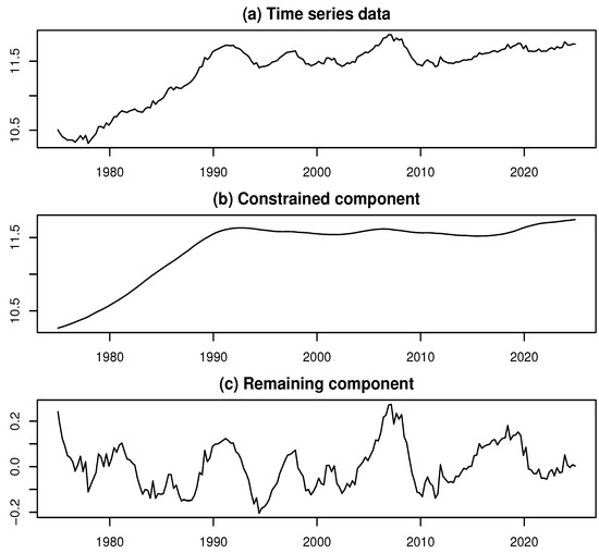
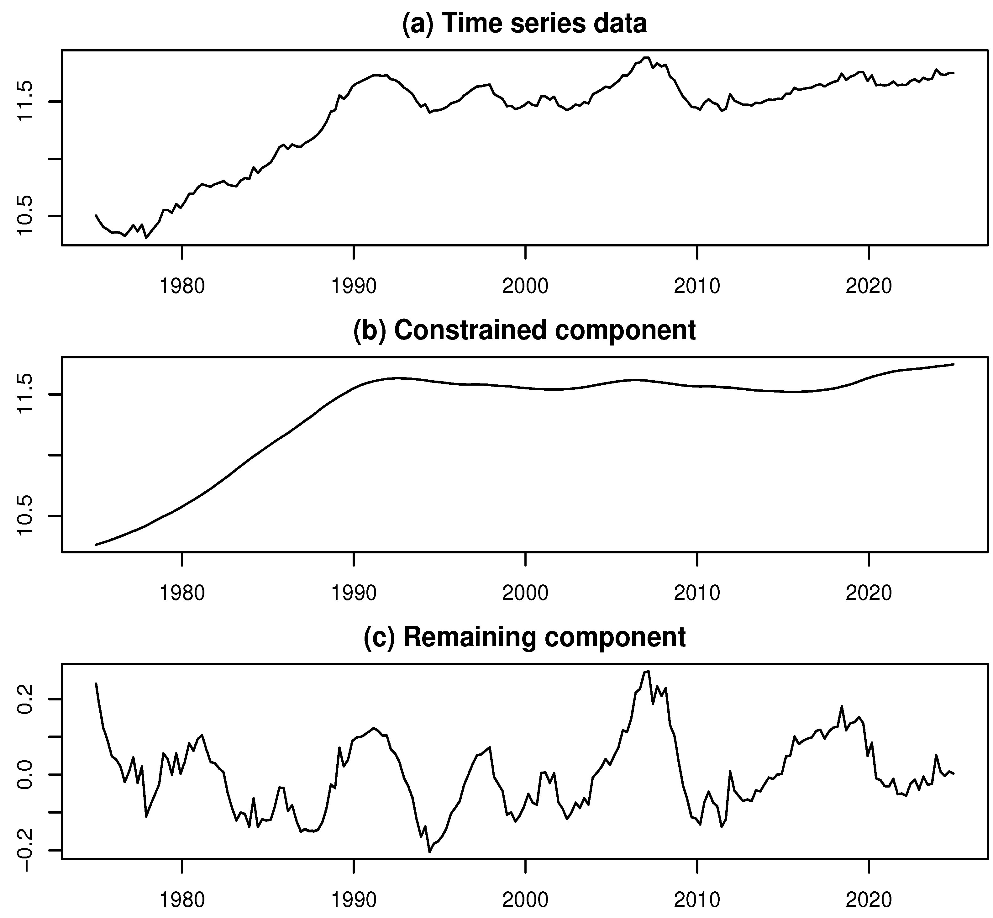
The time series of BE reflects levels of capital investment and is known to exhibit distinct structural characteristics. The original BE data were obtained from the website of the Japanese Cabinet Office (see [12]). This dataset comprises a monthly time series spanning from January 1975 to December 2024, totaling $N=600$ observations. Figure 1a presents a plot of the logarithmically transformed BE series (log-BE), which shows no prominent outliers in the time series.

Figure 1. Data and decomposed results for the log-BE time series.

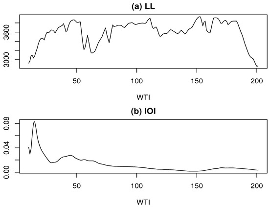
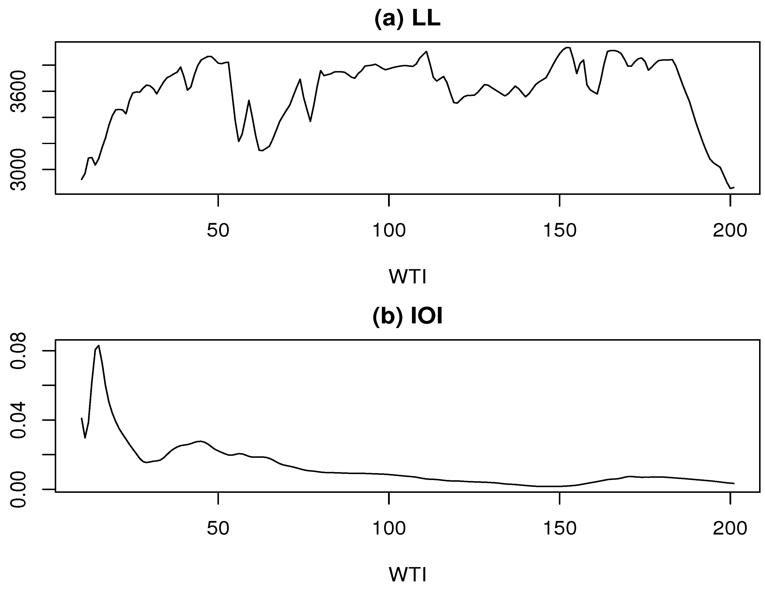
We applied the ML model approach to decompose the log-BE time series, conducting the decomposition for each value of k ranging from 3 to 202. As shown in Figure 2a, the log-likelihood (LL) exhibits local maxima at $k=47$, 111, and 152, with corresponding LL values of 3867.97, 3905.51, and 3936.10, respectively. Among these, the highest LL is achieved at $k=152$. Furthermore, Figure 2b shows that the IOI reaches its minimum near $k=152$. This further supports the adoption of $\widehat{k}=152$ as the estimate of k. These results indicate that the maximum likelihood estimate of k effectively captures a stable underlying structure.

Figure 2. Log-likelihood and IOI vs. WTI for the log-BE time series.

Thus, we performed the constrained-remaining components decomposition using $\widehat{k}=152$. Figure 1b,c illustrate the results of the decomposition for the log-BE time series, with Figure 1b showing the constrained component and Figure 1c presenting the remaining component.

Incidentally, to validate the results of this study, we refer to the state-space modeling approach introduced in [9]. In that work, the R function season is used to decompose a time series into three components: a trend, an AR component, and observation noise. When this function was applied to the log-BE series, the order of the trend component was estimated to be 2, and that of the AR component was estimated to be 4. Based on these estimates, the time series was then decomposed accordingly.

To align with the ML model framework, we treated the trend as the constrained component and regarded the sum of the AR component and observation noise as the remaining component. For each value of k, we computed the MISS values by comparing the decomposition results from the ML model approach with those obtained using the season function. The MISS reached its minimum around $k=11$, suggesting that the conventional state-space-based decomposition corresponds most closely to the ML model approach at this value of k. Notably, around $k=11$, the IOI value is approximately 0.08, which is near its maximum. This implies that, in comparison with the ML model approach, the component decomposition based on the state-space model lacks stability.

These findings suggest that the constrained component yields a highly smooth time series, effectively capturing the long-term trend in the log-BE data. Consequently, most short-term fluctuations are absorbed into the remaining component, which displays complex and irregular behavior. This observation provides a strong rationale for reapplying the ML model approach to further decompose the initial remaining component.

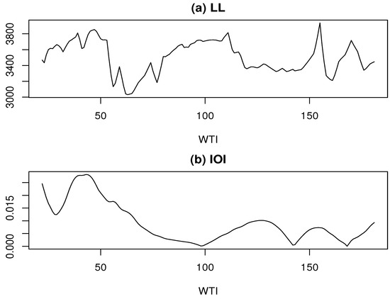
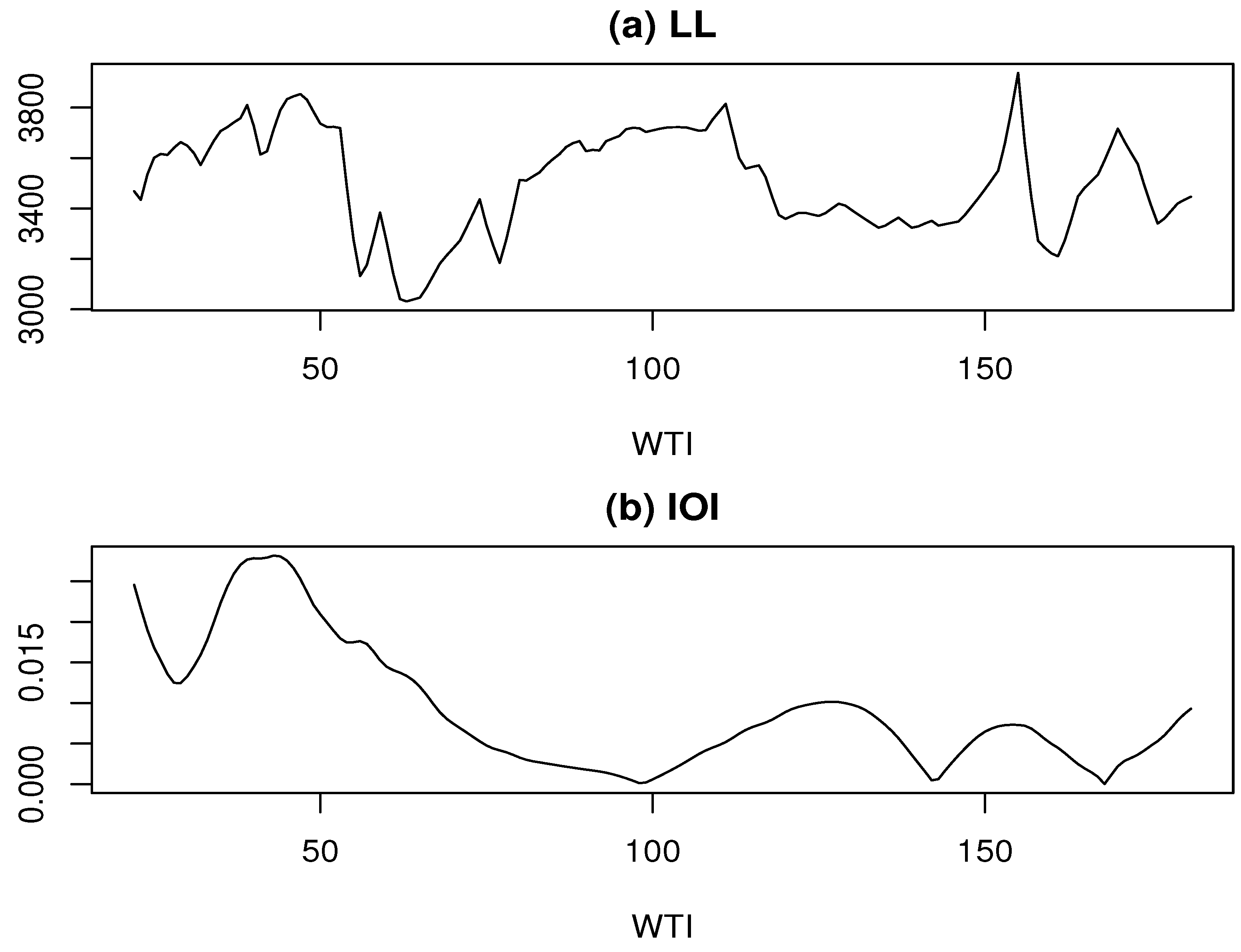
Thus, we further decomposed the initial remaining component using the ML model approach for each value of k ranging from 3 to 182. Similar to the first component decomposition, the LL exhibits local maxima at $k=47$, 111, and 155, with corresponding LL values of 3853.70, 3814.70, and 3937.52, respectively, as shown in Figure 3a. Among these, the highest LL is achieved at $k=155$.

Figure 3. Log-likelihood and IOI vs. WTI for the second component decomposition.

However, as shown in Figure 3b, the IOI values at these k points are elevated compared to their surroundings, suggesting that the most stable decomposition may not be achieved at these values of k. A closer examination of Figure 3b reveals a noticeable valley in the IOI at $k=97$. Although the LL value at this point is 3719.58—which is not exceptionally high—it remains relatively stable and elevated in the surrounding region. Therefore, we adopt $\widehat{k}=97$ as the estimate of k for the second component decomposition.

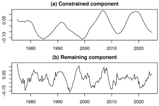
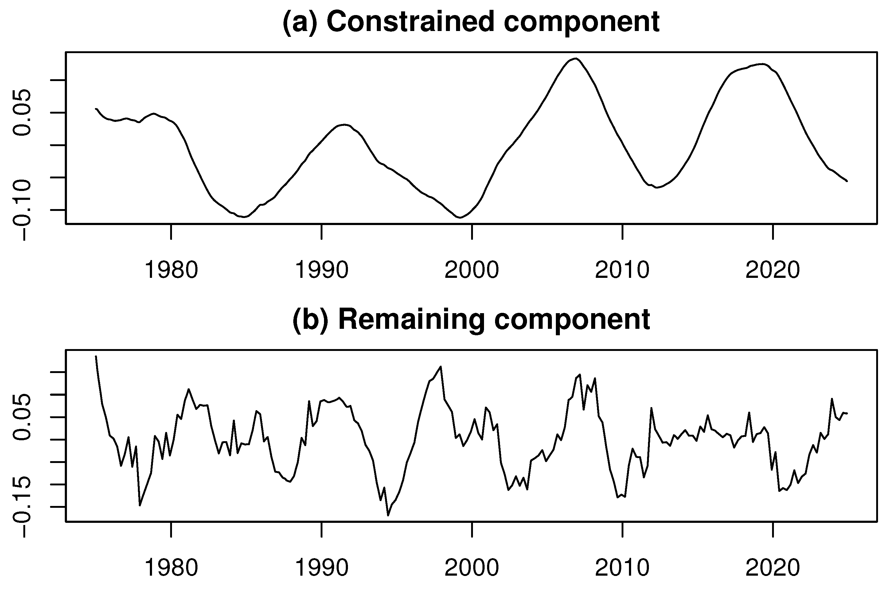
Figure 4 displays the results of the second component decomposition, which was applied to the initial remaining component obtained from the first decomposition. Figure 4a and Figure 4b show the constrained component and the remaining component, respectively.

Figure 4. Results of the second component decomposition.

The constrained component in the second decomposition, shown in Figure 4a, exhibits cyclical behavior with a period exceeding a decade, aligning with the characteristics of the Juglar cycle (see [13]). This point is particularly noteworthy: in this case, the time series being decomposed is itself a remaining component that contains cyclical fluctuations of various durations. As a result, the constrained component extracted in this step captures a smooth, long-period cyclical fluctuation.

Furthermore, the remaining component in the second decomposition, shown in Figure 4b, is characterized by short-term cyclical fluctuations. These findings further support the consistency of the results with business cycle theory and highlight the effectiveness of the proposed approach in identifying and analyzing business cycles (see [1]).

The results presented above suggest that incorporating additional metrics and estimation methods alongside the conventional maximum likelihood approach can lead to more stable decomposition outcomes. Naturally, the results of decomposition may vary depending on the number of components extracted and the choice of k values. This highlights the inherently data-driven and purpose-oriented nature of data analysis; trial and error, guided by the specific analytical objectives, is therefore indispensable.

4.2. Empirical Analysis of Industrial Production in Japan

This section presents an empirical analysis of the seasonally adjusted index of industrial production (SAIIP) in Japan as the second case study. Its purpose is to demonstrate the effectiveness of the reinforced EML model in detecting and estimating outliers in time series data.

The SAIIP data were obtained from the same source as the BE data analyzed in the first example. As a core indicator for assessing economic trends, the SAIIP is widely used in empirical research. Although outliers are not frequently observed, they may emerge in response to significant economic disturbances, reflecting the series’ sensitivity to abrupt changes in economic conditions.

To facilitate comparison with the empirical example in [7], we use the data as a monthly time series from January 1975 to December 2022, comprising a total of $N=576$ observations. A logarithmic transformation is applied to the SAIIP series, resulting in what we refer to as the log-SAIIP. The objective of this analysis is to investigate the time series behavior of the log-SAIIP.

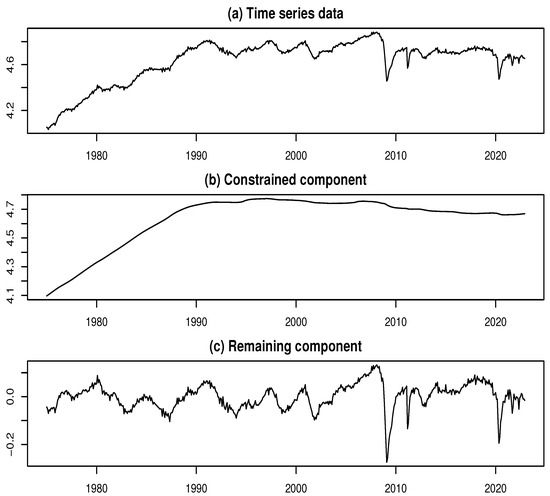
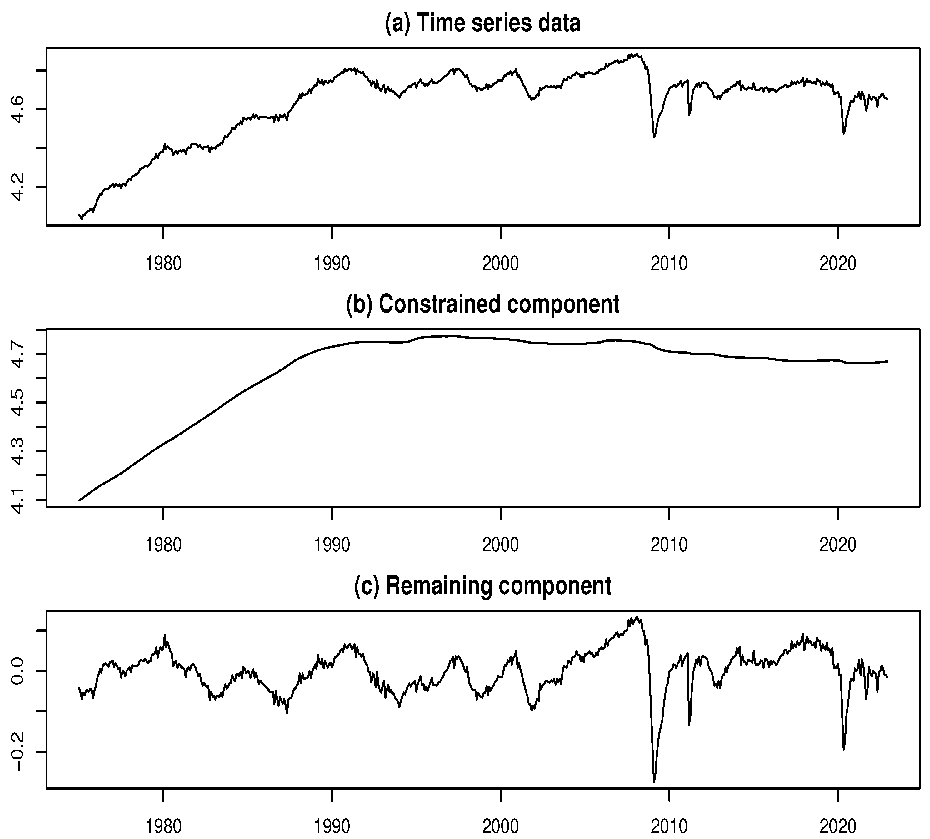
Figure 5a presents the time series plot of the log-SAIIP. Two prominent declines are clearly visible in the series. The first, occurring around February 2009, is attributable to the aftermath of the global financial crisis of 2007–2008. The second, around May 2020, reflects the impact of the COVID-19 pandemic. These sharp declines are likely associated with the presence of multiple outliers.

Figure 5. Data and decomposed results for the log-SAIIP time series.

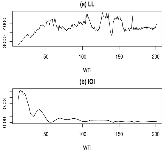
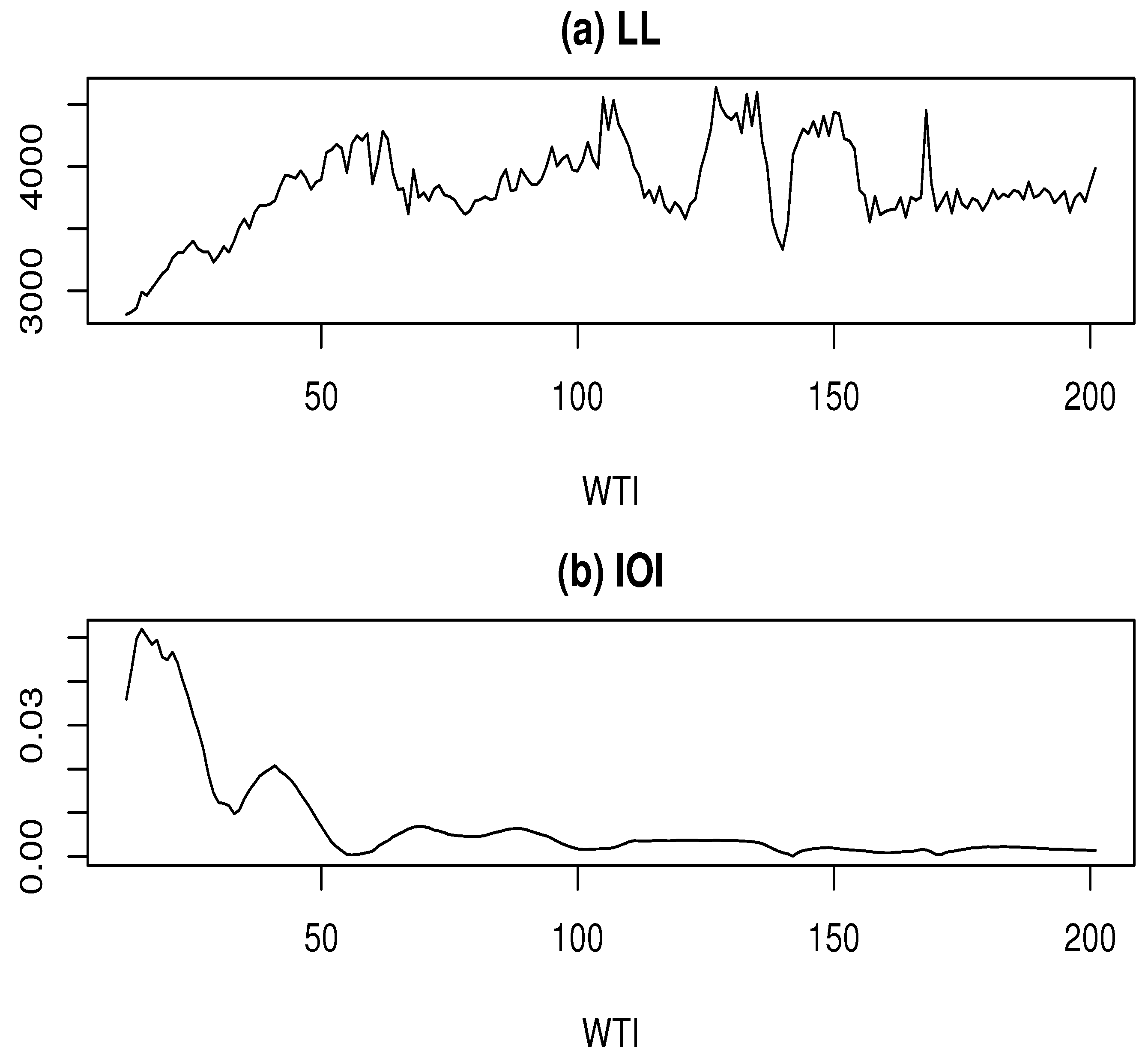
To determine the potential locations of outliers, we applied the ML model approach to decompose the log-SAIIP time series while ignoring the presence of outliers. This decomposition was performed for each value of k ranging from 3 to 202. As shown in Figure 6a, the LL exhibits many prominent local maxima. Notably, distinct peaks are observed at $k=15$, 25, 43, 62, 105, 127, and 150, corresponding to LL values of 2991.14, 3402.40, 3932.02, 4285.37, 4555.44, 4639.64, and 4438.77, respectively. In addition, a spike-like surge in LL is observed at $k=168$, which reaches a peak value of 4453.67. As seen in Figure 6b, and excluding the three points where $k<50$, the IOI values for these values of k remain generally low, with no significant differences observed.

Figure 6. Log-likelihood and IOI vs. WTI for the log-SAIIP time series.

Figure 5 shows, for reference, the component decomposition of the log-SAIIP time series using the ML model at $k=127$, where the maximum log-likelihood was achieved while ignoring outliers.

Figure 5b,c present the results of the constrained-remaining component decomposition using the ML model approach with $k=127$. In Figure 5b, the constrained component displays a smooth trend, whereas Figure 5c shows that the remaining component exhibits cyclical fluctuations, suggesting the presence of business cycles in Japan. Notably, a significant portion of the sharp declines observed around February 2009 and May 2020 is captured by the remaining component. These abrupt drops in the time series likely reflect the influence of outliers caused by sudden economic shocks. Therefore, the elements responsible for these variations should be identified and treated as outliers, as they may distort the analysis of business cycles.

Then, outlier detection and estimation were performed for k values of 15, 25, 43, 62, 105, 127, 150, and 168, with the upper limit on the number of potential outliers set to $M=35$. This procedure followed the AIC reduction maximization method introduced in Section 3.3. The results are summarized in Table 1. Notably, at $k=168$, no outliers were detected that would lead to a reduction in the AIC.

Table 1. Results of outlier detection and estimation.

WTI (k)	Estimate of Outlier Number	AIC Without Outliers	AIC with Outliers	Reduction in AIC
15	16	−5980.28	−6350.23	369.94
25	16	−6802.79	−7218.42	415.63
43	24	−7862.04	−8165.75	303.71
62	25	−8568.73	−8803.30	234.57
105	9	−9108.88	−9127.49	18.61
127	15	−9277.28	−9304.63	27.35
150	$1$	−8875.54	−8877.63	2.09

As shown in Table 1, among the various settings of k, the case with $k=25$ resulted in the largest AIC reduction of 415.63. Based on the AIC reduction maximization method, this setting was adopted for outlier detection and estimation with outliers incorporated. As a result, a total of $m=16$ outliers were detected, occurring at time points 556, 410, 558, 411, 412, 409, 413, 545, 546, 553, 401, 435, 400, 544, 402, and 403. Notably, the outliers were highly concentrated around 2009, and several were also identified in the first half of 2020.

Furthermore, based on the detected outlier locations and the corresponding estimation results, the log-SAIIP time series was adjusted to eliminate the effects of outliers. To determine the final value of k for component decomposition, the ML model approach was applied to the adjusted time series across a range of candidate k values, and the corresponding AIC values were calculated. The results are presented in Table 2.

Table 2. AIC value vs. k for the outlier-adjusted time series.

k Value	15	25	43	62	105	127	150
AIC value	−6347.9	−7218.4	−8043.7	−8685.9	−8987.9	−9162.2	−8567.6

As shown in Table 2, the minimum AIC was obtained at $k=127$, which is consistent with the maximum likelihood estimate obtained under the assumption that outliers are ignored. Therefore, $\widehat{k}=127$ was adopted as the final estimate of k, and the corresponding component decomposition results were regarded as the final estimates.

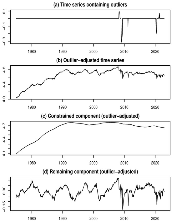
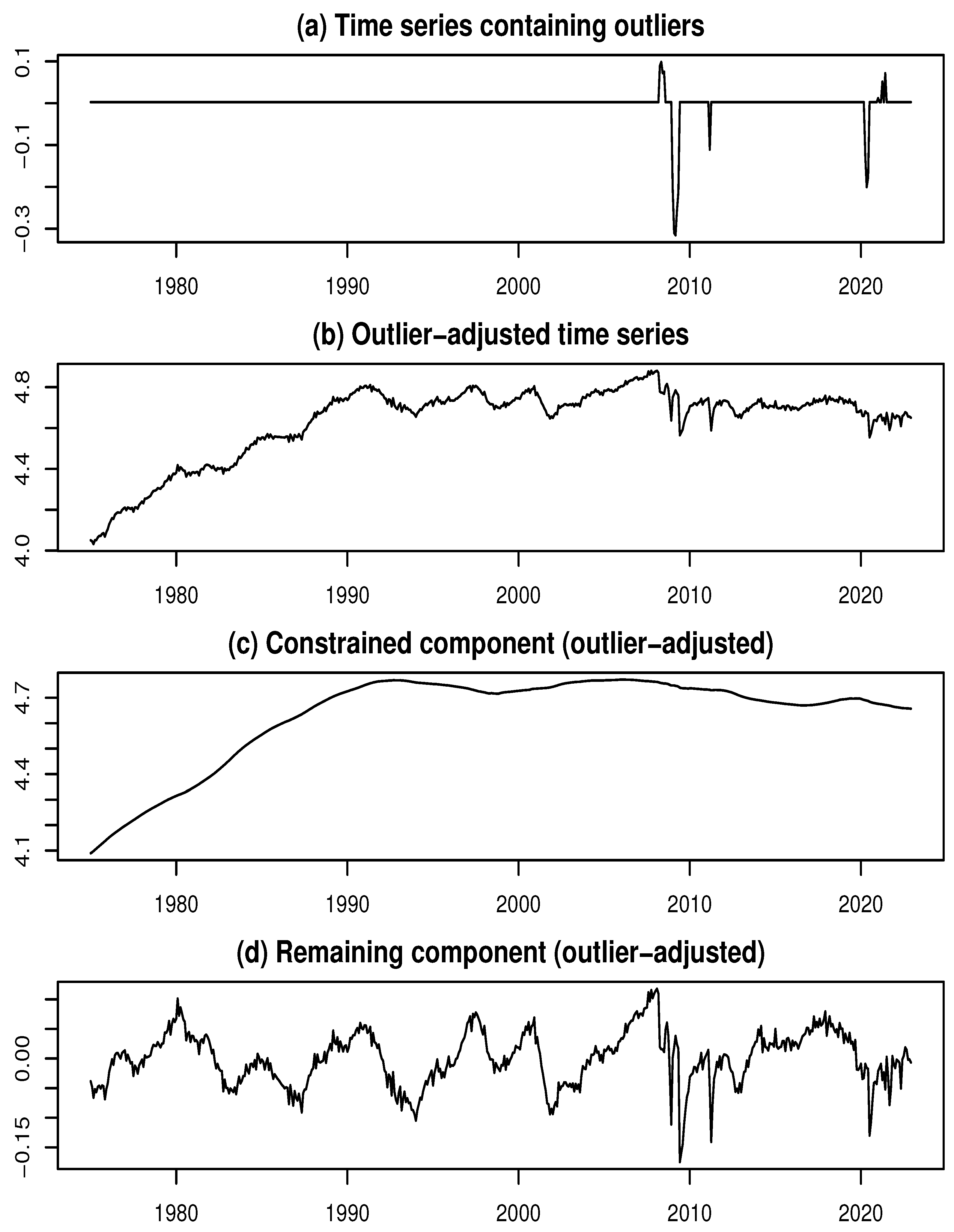
Finally, we performed component decomposition on the outlier-adjusted time series. Figure 7a shows the time series containing the estimated outliers, while Figure 7b presents the outlier-adjusted time series. Figure 7c and Figure 7d display the estimated constrained and remaining components, respectively, based on the adjusted data. Compared to the initial estimate of the remaining component shown in Figure 5c, the results in Figure 7d exhibit a marked improvement in uniformity.

Figure 7. Final results of decomposition for the log-SAIIP time series.

As a reference for comparison, we again present the main results obtained in [7]. In that study, an EML model approach—reviewed in Section 2.2—was employed to detect and estimate outliers. The number of outliers was estimated as $m=22$, based on a method that determined outlier locations in order of the squared standardized outliers. This procedure yielded a minimum AIC value of $-8009.5$.

Thus, by employing the present AIC reduction maximization method, the AIC was reduced by 1152.7, thereby enhancing the reliability of the estimation results. Although the difference between the component decomposition results obtained in [7] and those shown in Figure 7 is not readily discernible in the graphical representation and is therefore omitted, a comparison based on the numerical values of the evaluation metrics is presented below.

Accordingly, we evaluate the decomposition results using the index of symmetry and uniformity (ISU), proposed by [14], as a benchmark. For a given time series, the ISU is defined as the logarithmic ratio of the standard deviation of the absolute values of the series to the standard deviation of the original series. In the case of the outlier-adjusted remaining component, a larger standard deviation of the absolute values indicates that the constrained component has become smoother after the outlier adjustment. This suggests that the impact of outliers on the decomposition result is weaker, resulting in greater stability—an outcome that is desirable. Conversely, a smaller standard deviation of the absolute values implies greater symmetry around the mean, which also reflects a reduced influence of outliers on the remaining component. Therefore, the decomposition results are evaluated based on the minimum ISU criterion applied to the outlier-adjusted remaining component.

Based on the above findings, the following results were obtained. For the result derived using the method proposed by [7], the ISU was $-0.2386$. In contrast, the result obtained through the present AIC reduction maximization method yielded a lower ISU value of $-0.2492$. This improvement, as assessed using the minimum ISU criterion, highlights the advantage of the AIC reduction maximization method.

Considering these outcomes, a key feature of the proposed method lies in its thorough application of the ML model approach, which makes it particularly promising for effectively handling outliers in the constrained-remaining components decomposition.

5. Summary and Discussion

We began by reviewing the ML model approach proposed by [1], along with its extension, the EML model approach introduced by [7], which together formed the theoretical foundation of this study. Building on these frameworks, we developed several methodological advancements, which are particularly aimed at improving outlier detection and estimation.

Although the maximum likelihood estimation for the WTI was originally developed as a practical tool in [1], the present study clarified its theoretical significance in the decomposition of constrained and remaining components. This theoretical foundation contributed to improved estimation stability and enhanced both the interpretability and robustness of the model. To further support model evaluation, we introduced new metrics that provided a broader perspective than conventional likelihood-based approaches. Notably, the IOI—constructed from the newly proposed SISS—served as a powerful supplementary criterion alongside the log-likelihood and strengthened the credibility of the maximum likelihood estimation results.

Other key methodological developments included bidirectional processing strategies that integrated forward and backward decompositions. Averaging the results from both directions led to more stable and reliable component estimates. We also proposed a novel three-step approach for outlier detection: identifying potential outlier locations, estimating the number and values of outliers, and updating their locations systematically. This process employed the AIC to iteratively refine the model by determining outlier locations that reduced the AIC and improved model fit.

A major contribution in this regard was the AIC reduction maximization method, which accounted for interdependencies among outliers and automatically determined their optimal number and locations. This approach significantly enhanced the model’s explanatory and predictive performance, strengthening its ability to handle outliers in time series data.

The empirical analyses provided strong evidence of the practical utility and robustness of the proposed method. The first example involved analyzing data on business expenditures for new plants and equipment in Japan from January 1975 to December 2024. This example demonstrated the effectiveness of maximum likelihood estimation supported by the IOI criterion. By repeatedly applying the ML model approach, the target time series was successfully decomposed into a trend and two cyclical components. A detailed examination of Japan’s business cycles based on these two cyclical components revealed fluctuations consistent with the Juglar cycle.

The second example applied the method to the seasonally adjusted index of industrial production from January 1975 to December 2022. In this case, the focus was on detecting and estimating outliers caused by socio-economic shocks. The AIC reduction maximization method successfully identified 16 outliers in the target data and produced a more reliable component decomposition. Evaluation metrics, including the ISU, confirmed that the proposed approach outperformed previous methods in terms of both robustness and the smoothness of the resulting components.

Taken together, these results underscored the importance of properly addressing outliers in time series data. When left untreated, outliers could significantly distort component decomposition, leading to misinterpretations of structural dynamics such as business cycles. Traditional detection techniques often lacked the flexibility to capture context-dependent outliers or to quantify their overall impact. In contrast, the proposed method systematically identified and adjusted for outliers using model-based criteria, thereby enhancing both the accuracy and interpretability of the estimation results.

Ultimately, while the proposed framework was general and contributed to the broader field of time series decomposition and outlier detection, its primary aim was to enhance the precision of business cycle analysis and lay the groundwork for causal interpretations of outliers. In particular, by identifying outliers as potential signals of policy interventions or exogenous shocks, the method opened new avenues for evaluating the sources and impacts of macroeconomic fluctuations. This established a bridge between statistical modeling and economic interpretation, highlighting the analytical power of the reinforced ML and EML model approaches.

References

- Kyo, K.; Kitagawa, G. A moving linear model approach for extracting cyclical variation from time series data. J. Bus. Cycle Res. 2023, 19, 373–397. [Google Scholar] [CrossRef] [Scilit]
- Kyo, K.; Noda, H.; Fang, F. An integrated approach for decomposing time series data into trend, cycle and seasonal components. Math. Comput. Model. Dyn. Syst. 2024, 30, 792–813. [Google Scholar] [CrossRef] [Scilit]
- Ren, H.; Xu, B.; Wang, Y.; Yi, C.; Huang, C.; Kou, X.; Xing, T.; Yang, M.; Tong, J.; Zhang, Q. Time-series anomaly detection service at Microsoft. In Proceedings of the KDD ’19: The 25th ACM SIGKDD Conference on Knowledge Discovery and Data Mining, Anchorage, AK, USA, 4–8 August 2019. [Google Scholar] [CrossRef] [Scilit]
- Vishwakarma, G.K.; Paul, C.; Elsawah, A.M. An algorithm for outlier detection in a time series model using backpropagation neural network. J. King Saud Univ.—Sci. 2020, 32, 3328–3336. [Google Scholar] [CrossRef] [Scilit]
- Jamshidi, E.J.; Yusup, Y.; Kayode, J.S.; Kamaruddin, M.A. Detecting outliers in a univariate time series dataset using unsupervised combined statistical methods: A case study on surface water temperature. Ecol. Inform. 2022, 69, 101672. [Google Scholar] [CrossRef] [Scilit]
- Kyo, K. An approach for the identification and estimation of outliers in a time series with a nonstationary mean. In Proceedings of the 2023 World Congress in Computer Science, Computer Engineering, & Applied Computing (CSCE’23), Las Vegas, NV, USA, 24–27 July 2023; IEEE Computer Society: Washington, DC, USA, 2003; pp. 1477–1482. [Google Scholar]
- Kyo, K. Enhancing business cycle analysis by integrating anomaly detection and components decomposition of time series data. Stat. Methods Appl. 2025, 34, 129–154. [Google Scholar] [CrossRef] [Scilit]
- Kyo, K.; Noda, H. Analyzing mechanisms of business fluctuations involving time-varying structure in Japan: Methodological proposition and empirical study. Comput. Econ. 2025. [Google Scholar] [CrossRef] [Scilit]
- Kitagawa, G. Introduction to Time Series Modeling with Application in R, 2nd ed.; CRC Press: Boca Raton, FL, USA, 2020. [Google Scholar]
- Kitagawa, G.; Gersch, W. A smoothness priors state space modeling of time series with trend and seasonality. J. Am. Stat. Assoc. 1984, 79, 378–389. [Google Scholar]
- Akaike, H. A new look at the statistical model identification. IEEE Trans. Autom. Control 1974, AC-19, 716–723. [Google Scholar] [CrossRef] [Scilit]
- Japanese Cabinet Office. Coincident Index. 2025. Available online: https://www.esri.cao.go.jp/en/stat/di/di-e.html (accessed on 6 May 2025).
- Schumpeter, J.A. Business Cycles: A Theoretical, Historical, and Statistical Analysis of the Capitalist Process; McGraw-Hill: New York, NY, USA, 1939; Volumes I & II. [Google Scholar]
- Kyo, K. Identifying and estimating outliers in time series with nonstationary mean through multi-objective optimization method. In Big Data, Data Mining and Data Science: Algorithms, Infrastructures, Management and Security; De Gruyter: Berlin, Germany, 2025. [Google Scholar]
Disclaimer/Publisher’s Note: The statements, opinions and data contained in all publications are solely those of the individual author(s) and contributor(s) and not of MDPI and/or the editor(s). MDPI and/or the editor(s) disclaim responsibility for any injury to people or property resulting from any ideas, methods, instructions or products referred to in the content. |
© 2025 by the author. Licensee MDPI, Basel, Switzerland. This article is an open access article distributed under the terms and conditions of the Creative Commons Attribution (CC BY) license (https://creativecommons.org/licenses/by/4.0/).