Abstract
Here, we consider the stochastic graphene sheets model (SGSM) forced by multiplicative noise in the Itô sense. We show that the exact solution of the SGSM may be obtained by solving some deterministic counterparts of the graphene sheets model and combining the result with a solution of stochastic ordinary differential equations. By applying the extended tanh function method, we obtain the soliton solutions for the deterministic counterparts of the graphene sheets model. Because graphene sheets are important in many fields, such as electronics, photonics, and energy storage, the solutions of the stochastic graphene sheets model are beneficial for understanding several fascinating scientific phenomena. Using the MATLAB program, we exhibit several 3D graphs that illustrate the impact of multiplicative noise on the exact solutions of the SGSM. By incorporating stochastic elements into the equations that govern the evolution of graphene sheets, researchers can gain insights into how these fluctuations impact the behavior of the material over time.
MSC:
60H15; 60H10; 35Q51; 35A20
1. Introduction
Nonlinear evolution equations (NLEEs) provide a powerful framework for analyzing complex systems across multiple disciplines, revealing profound insights into the behavior and evolution of natural and engineered systems. These equations arise in various scientific fields, including fluid dynamics, plasma physics, biology, and finance.
Solutions to NLEEs enable us to model complex phenomena, including fluid dynamics, heat transfer, quantum mechanics, financial mathematics, and more. The importance of these solutions lies in their ability to provide insight into the behavior of systems governed by these equations, allowing for predictions and optimizations crucial for both theoretical understanding and practical applications. Recently, many useful and efficient techniques have been developed to obtain exact solutions for NLEEs, such as the sine-Gordon expansion technique [1], the F-expansion method [2], the auxiliary equation scheme [3], Jacobi elliptic function expansion [4,5], -expansion [6,7], the sine–cosine method [8], the exp-function method [9], the -expansion method [10], the perturbation method [11,12], etc.
Moreover, NLEEs are widely used in research on graphene sheets. Graphene, a single layer of carbon atoms arranged in a two-dimensional honeycomb lattice, has garnered substantial interest in recent years due to its unique electronic, mechanical, and thermal properties [13,14,15]. Among the various phenomena observed in graphene, the behavior of nonlinear evolution equations plays a crucial role in understanding wave propagation, stability, and interactions within this material. Nonlinear evolution equations describe systems where the output is not directly proportional to the input, leading to complex dynamics that are especially relevant in the context of graphene. Such equations can model diverse phenomena, from solitons and shock waves to the formation of defects and the modulation of electronic states under external stimuli.
The (2 + 1)-dimensional graphene sheets model (GSM) is expressed in the following form [16]:
where denotes the wave function’s amplitude in the graphene sheet; represents the rate of change in ’s slope in the x-direction over t; indicates the spatial dispersion term; represents a self-interaction of the wave function along x; represents linear amplification along x; is the diffusion of the wave function along the spatial direction y; and and are real constants. Recently, Khater et al. [16] obtained the exact solutions of Equation (1) by employing several methods, such as the Khater II, Khater III, and generalized rational methods.
Nonlinear evolution equations offer great insights into graphene’s behavior, but they sometimes fail to account for the messy realities we encounter outside of a neat theoretical model. Therefore, by incorporating a stochastic term, we are essentially recognizing that randomness can lead to richer insights and better predictions because it helps capture the uncertainty that is often ignored in deterministic models. As a result, here we consider Equation (1) forced by multiplicative noise in the Itô sense as follows:
where is the Brownian motion process (see Section 2 for details) and is a real number representing the intensity of noise. Also, refers to the variation in the magnitude of noise present in a system where the noise is proportional to the level of the signal being analyzed. The stochastic term, , arises as a perturbation term when we replace in a differential form of Equation (1) with A similar stochastic term, would appear if with
Also, we can obtain the same results when we replace the constant with
The objective of this paper is to determine the exact stochastic solutions of the stochastic graphene sheets model (SGSM) (2). By applying Itô calculus and transformation techniques, we decompose the SGSM into two equations, a deterministic graphene sheets model (DGSM) and a stochastic ordinary differential equation. After that, we can find the solutions of DGSM by utilizing the expanded tanh function method. Many significant scientific phenomena may be examined using the achieved solutions, since the SGSM (2) has essential applications. We give several graphical representations using the MATLAB program to illustrate the practical use of the solutions of the SGSM (2).
This paper is arranged as follows: In the next section, we state some properties of Brownian motion and provide a lemma for decomposing the SGSM (2) into two equations, the deterministic counterparts of the graphene sheets model and a stochastic ordinary differential equation. In Section 3, the solutions of the deterministic counterparts of the graphene sheets model are obtained. In Section 4, the stochastic solutions of the SGSM (2) are acquired. Finally, the study’s findings are given.
2. Preliminaries
In this section, we follow the results stated in [17]. Let {} be Brownian motion defined on the probability space (). Brownian motion satisfies the following conditions [18]: (I) has continuous trajectories, (II) , (III) has a normal distribution, and (IV) has stationary, independent increments.
We provide the following lemma to show that the exact solution of the SGSM (2) may be acquired by solving some deterministic equivalents of the graphene sheets model and combining the result with a solution of stochastic ordinary differential equations.
Lemma 1.
The SGSM (2) has the solutions where is the solution of the following deterministic graphene sheets model (DGSM):
and are the solutions of
with the initial values
where , and is a continuous bounded function.
Proof.
By applying the Itô formula (see [19])
Using (3)–(5), we get
where we use and ( Since , we obtain (2). □
3. Solutions of DGSM
To create the wave equation for the DGSM (3), we utilize the following wave transformation:
where is a deterministic function; is the wave number component in the x direction; is the wave number component in the y direction; and is the wave speed. We see that
Plugging Equation (6) into Equation (3) and using (7), we attain
After twice integrating Equation (8) and neglecting the integration constant, we obtain
where
Now, we use the extended tanh function method [20]. Assume the solution to Equation (9) is
where solves the Riccati equation
where are undefined constants to be determined, and is a real constant. The Riccati Equation (11) has several types of solutions, which are as follows:
and
Now, it is necessary to balance with in Equation (9) in order to calculate M as follows
Rewriting Equation (10) with , we get
Putting Equation (15) into Equation (9), we get
Assigning zero to the coefficients of every power of yields
and
These equations can be solved to attain the next two sets of solutions:
Set I:
Set II:
For Set I: Equation (9) has the following solution:
Since by using (13), we get
and
Thus, the DGSM (3) has the following soliton solutions:
and
For Set II: Equation (9) has the solution
Since by using (13), we get
and
Therefore, the DGSM (3) has the following solutions:
and
4. Exact Solutions of SGSM
First, integrate Equations (4) and (5) from 0 to t to obtain
To find the exact solutions of the SGSM (2), there are many cases that must be solved:
Case 1 (see Equation (18)):
Therefore, the solution of the SGSM (2) takes, using (22), the form
Case 2 (see Equation (19)):
Therefore, the solution of the SGSM (2) takes, using (22), the form
Case 3 (see Equation (20)):
Therefore, the solution of the SGSM (2) takes, using (22), the form
Case 4 (see Equation (21)):
Therefore, the solution of the SGSM (2) takes, using (22), the form
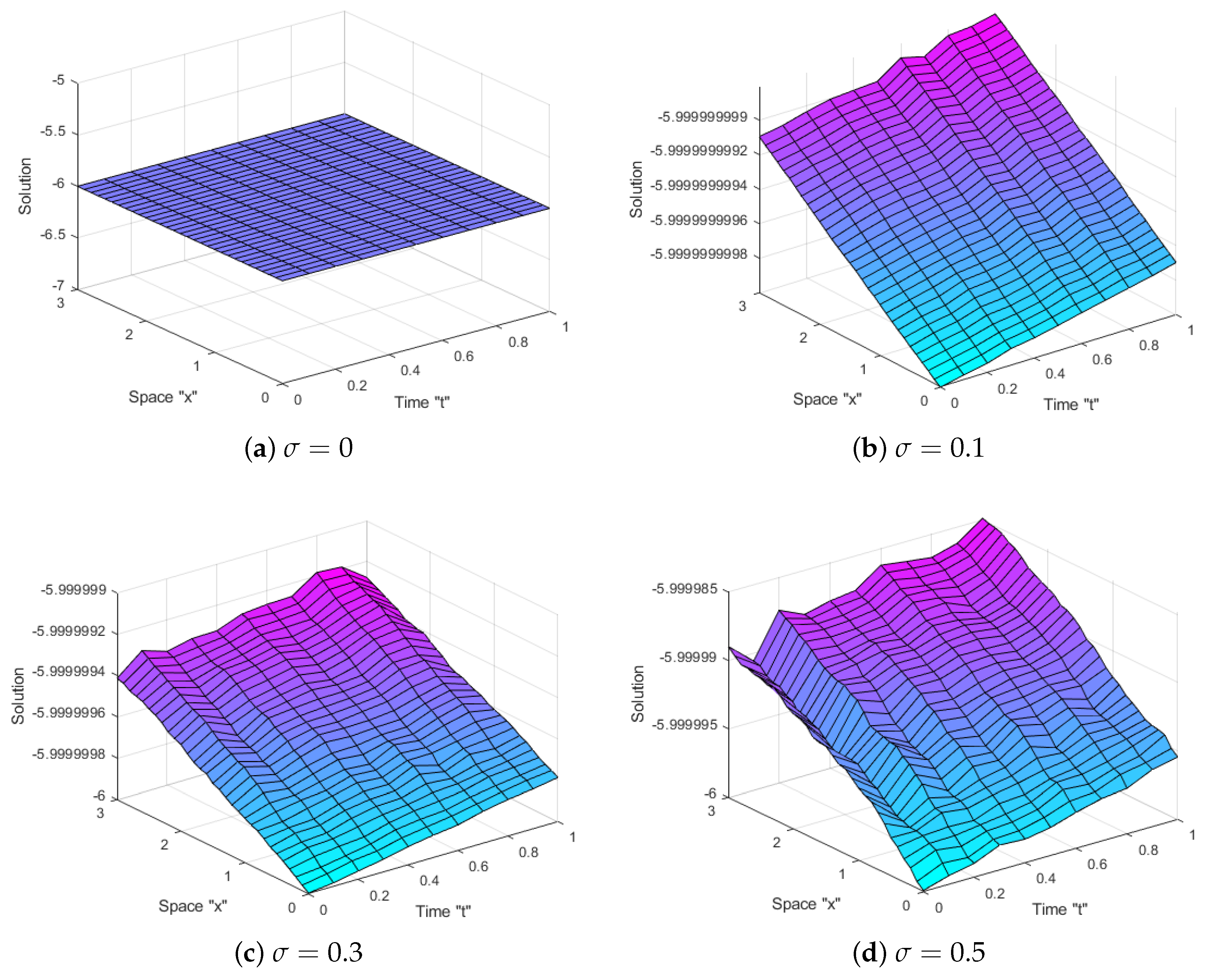
To simulate Figure 1 and Figure 2, we set ; to discretize the Brownian motion over From these figures, we conclude that when the intensity of noise, increases, the surface starts to fluctuate more much more.
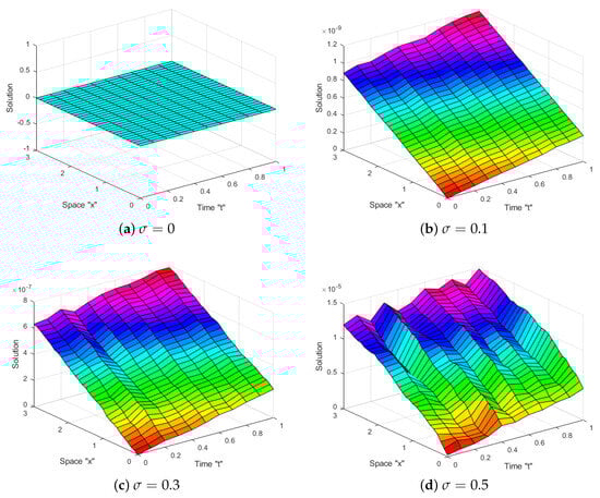
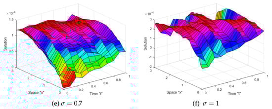
Figure 1.
This figure displays the 3D shape for the amplitude solution stated in Equation (23) with and with distinct .
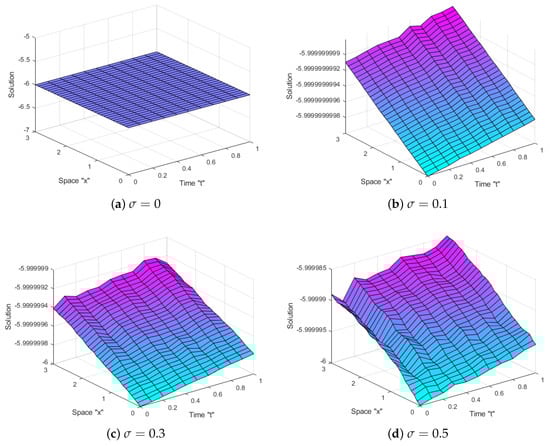
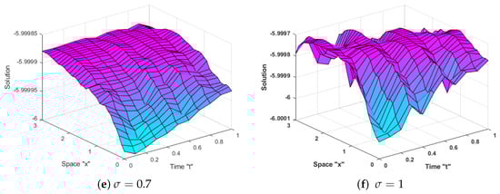
Figure 2.
This figure displays the 3D shape for the amplitude solution stated in Equation (25) with and with distinct .
5. Conclusions
In this work, we investigated the solutions of the stochastic graphene sheets model (SGSM) forced in the Itô sense by multiplicative noise. By using Itô calculus and transformation techniques, we divided the SGSM into two equations: a stochastic ordinary differential equation and a deterministic graphene sheets model (DGSM). We obtained the soliton solutions for the DGSM by applying the extended tanh function method. After that, the exact solution of the SGSM was obtained by combining the solutions of the DGSM and the solutions of the stochastic ordinary differential equation. The acquired solutions of the SGSM (2) are helpful in comprehending a number of interesting scientific phenomena, since graphene sheets are significant in several areas, including electronics, photonics, and energy storage. Also, we presented a number of simulations using the MATLAB R2022b software (for more detail, see [21]) to demonstrate how the solutions of the SGSM may be used practically. Based on these results, we concluded that the surface fluctuates due to the presence of multiplicative noise. In future work, we can consider an SGSM (2) with a two-dimensional Brownian motion process. Also, we can obtain the exact solutions for a graphene sheets model (1) with additive noise.
Author Contributions
Conceptualization, T.S.H., R.S., H.A. and M.S.A.; methodology, W.W.M., T.S.H., R.S., H.A. and M.S.A.; software, W.W.M.; validation, W.W.M., T.S.H., R.S., H.A. and M.S.A.; formal analysis, T.S.H., R.S., H.A. and M.S.A.; data curation, T.S.H., R.S., H.A. and M.S.A.; writing—original draft preparation, W.W.M., T.S.H., R.S., H.A. and M.S.A.; writing—review and editing, W.W.M.; visualization, T.S.H., R.S., H.A. and M.S.A.; supervision, W.W.M.; project administration, W.W.M.; funding acquisition, W.W.M. All authors have read and agreed to the published version of the manuscript.
Funding
This research has been funded by Scientific Research Deanship at the University of Ha’il-Saudi Arabia through project number RG-24097.
Informed Consent Statement
Not applicable.
Data Availability Statement
The original contributions presented in this study are included in this article; further inquiries can be directed to the corresponding author.
Conflicts of Interest
The authors declare no conflicts of interest.
References
- Baskonus, H.M.; Bulut, H.; Sulaiman, T.A. New complex hyperbolic structures to the lonngren-wave equation by using sine-gordon expansion method. Appl. Math. Nonlinear Sci. 2019, 4, 129–138. [Google Scholar] [CrossRef]
- Lu, B. The first integral method for some time fractional differential equations. J. Math. Anal. Appl. 2012, 395, 684–693. [Google Scholar] [CrossRef]
- Jiong, S. Auxiliary equation method for solving nonlinear partial differential equations. Phys. Lett. A 2003, 309, 387–396. [Google Scholar]
- Yan, Z.L. Abunbant families of Jacobi elliptic function solutions of the dimensional integrable Davey-Stewartson-type equation via a new method. Chaos Solitons Fractals 2003, 18, 299–309. [Google Scholar] [CrossRef]
- Mohammed, W.W.; Cesarano, C.; Al-Askar, F.M. Solutions to the (4+1)-Dimensional Time-Fractional Fokas Equation with M-Truncated Derivative. Mathematics 2023, 11, 194. [Google Scholar] [CrossRef]
- Wang, M.L.; Li, X.Z.; Zhang, J.L. The (G′/G)-expansion method and travelling wave solutions of nonlinear evolution equations in mathematical physics. Phys. Lett. A 2008, 372, 417–423. [Google Scholar] [CrossRef]
- Zhang, H. New application of the (G′/G)-expansion method. Commun. Nonlinear Sci. Numer. Simul. 2009, 14, 3220–3225. [Google Scholar] [CrossRef]
- Wazwaz, A.M. The sine-cosine method for obtaining solutions with compact and noncompact structures. Appl. Math. Comput. 2004, 159, 559–576. [Google Scholar] [CrossRef]
- He, J.H.; Wu, X.H. Exp-function method for nonlinear wave equations. Chaos Solitons Fractals 2006, 30, 700–708. [Google Scholar] [CrossRef]
- Khan, K.; Akbar, M.A. The exp(−ϕ(ς))-expansion method for finding travelling wave solutions of Vakhnenko-Parkes equation. Int. J. Dyn. Syst. Differ. Equ. 2014, 5, 72–83. [Google Scholar]
- Mohammed, W.W. Approximate solution of the Kuramoto-Shivashinsky equation on an unbounded domain. Chin. Ann. Math. Ser. B 2018, 39, 145–162. [Google Scholar] [CrossRef]
- Mohammed, W.W.; Iqbal, N.; Botmart, T. Additive Noise Effects on the Stabilization of Fractional-Space Diffusion Equation Solutions. Mathematics 2022, 10, 130. [Google Scholar] [CrossRef]
- Taya, S.A.; Daher, M.G.; Almawgani, A.H.M.; Hindi, A.T.; Colak, I.; Patel, S.K.; Pal, A. Absorption Properties of a One-Dimensional Photonic Crystal with a Defect Layer Composed of a Left-Handed Metamaterial and Two Monolayer Graphene. Phys. Status Solidi Appl. Res. 2023, 220, 2300164. [Google Scholar] [CrossRef]
- Bradley, A.N.; Thorp, S.G.; Mayonado, G.; Coporan, S.A.; Elliott, E.; Graham, M.W. Photoreduced graphene oxide recovers graphene hot electron cooling dynamics. Phys. Rev. B 2023, 107, 224309. [Google Scholar] [CrossRef]
- Model, J.C.M.; Veit, H.M. Development of a More Sustainable Hybrid Process for Lithium and Cobalt Recovery from Lithium Ion Batteries. Minerals 2023, 13, 798. [Google Scholar] [CrossRef]
- Khater, M.M.A.; Alfalqi, S.H.; Vokhmintsev, A. High-Precision computational solutions for nonlinear evolution models in graphene sheets. Sci. Rep. 2025, 15, 4013. [Google Scholar] [CrossRef] [PubMed]
- Exact solutions of stochastic Burgers–Korteweg de Vries type equation with variable coefficients. Partial Differ. Equ. Appl. Math. 2024, 11, 100753. [CrossRef]
- Calin, O. An Informal Introduction to Stochastic Calculus with Applications; World Scientific: Singapore, 2015. [Google Scholar]
- Kloeden, P.E.; Platen, E. Numerical Solution of Stochastic Differential Equations; Springer: Berlin/Heidelberg, Germany, 1992. [Google Scholar]
- Fan, E. Extended tanh-function method and its applications to nonlinear equations. Phys. Lett. A 2000, 277, 212–218. [Google Scholar] [CrossRef]
- Higham, D.J. An algorithmic introduction to numerical simulation of stochastic differential equations. SIAM Rev. 2001, 43, 525–546. [Google Scholar] [CrossRef]


Disclaimer/Publisher’s Note: The statements, opinions and data contained in all publications are solely those of the individual author(s) and contributor(s) and not of MDPI and/or the editor(s). MDPI and/or the editor(s) disclaim responsibility for any injury to people or property resulting from any ideas, methods, instructions or products referred to in the content. |
© 2025 by the authors. Licensee MDPI, Basel, Switzerland. This article is an open access article distributed under the terms and conditions of the Creative Commons Attribution (CC BY) license (https://creativecommons.org/licenses/by/4.0/).