Convergence and ω²-Stability Analysis of a Hybrid-Type Iterative Scheme with Application to Functional Delay Differential Equations

Abstract

The purpose of this article is to analyze a hybrid-type iterative algorithm for a class of generalized non-expansive mappings satisfying the Garcia-Falset property in uniformly convex Banach spaces. Some existing results for such mappings have been obtained using the given algorithm. The ${\omega }^2$-stability of the iterative process is also studied. Using some examples, numerical experiments are conducted by comparing this iterative algorithm with different well-known iterative schemes. It is concluded that this iterative algorithm converges faster to the fixed point and is preferable over the previously known iterative schemes using the Garcia-Falset property. A weak solution of the Volterra–Stieltjes-type delay functional differential equation is presented to demonstrate the significance of the proposed results.

1. Introduction

Fixed point theory deals with the study of conditions that guarantee the existence and approximation of the solutions of linear and nonlinear operator equations. The development of fixed point iterative algorithms to approximate the solution of certain operator equations is another domain of fixed point theory. These iterative algorithms are classified based on their stability, data dependency, rate of convergence, time and space complexities, and well-posedness.

Banach contraction principle (BCP), a well-known result in metric fixed point theory, applies to a large range of problems dealing with the existence and approximation of the solution of nonlinear operator equations such as differential and integral equations. BCP has some limitations as well. A natural extension of Banach contraction mapping is a non-expansive mapping whose fixed points cannot be approximated through the Picard iteration algorithm employed in BCP, refer to [1]. Indeed, it does not apply to several important classes of mappings that arise in modeling different convex optimization problems. Therefore, this principle has been generalized and extended by weakening the contraction condition. Kirk [2], Browder [3], and Gohde [4] established the existence of fixed points of non-expansive mappings defined on a specific subset of a Banach space satisfying certain geometric conditions. It was proved in 1955 that Picard’s iteration for non-expansive mappings may not converge to a fixed point [5]. For the approximation of fixed points in these mappings, numerous iterative processes have been introduced, for instance, by Mann [6], Ishikawa [7], Abbas and Nazir [8], Thakur et al. [9], and Picard–Mann [10].

Non-expansive mappings were extended by Suzuki [11] and Garcia-Falset et al. [12], which gave rise to two classes of generalized non-expansive mappings: the Suzuki mapping, which is the class of mappings that satisfy property C, and the Garcia-Falset mappings, which satisfy property E, a property that is weaker than the property C. The concept of Suzuki mapping is weaker than non-expansive mappings but stronger than quasi-non-expansive mappings. Similarly, the notion of Garcia-Falset mapping is weaker than Suzuki mappings [11] but not from quasi-non-expansive mappings, as shown by Proposition 1 and Example 1 below. Several authors presented examples on $\mathbb{R}$, ${\mathbb{R}}^2$, and on some infinite-dimensional spaces to show the inclusivity of Suzuki mappings [9,11,13]. Using three-step iterative methods, results for the existence of fixed points and convergence behavior were studied for the above-mentioned generalized non-expansive mappings [14,15,16].

Over the last few years, different iterative algorithms have been presented to obtain a faster rate of convergence. Moreover, the stability results and data dependency of these algorithms have also been studied (see, for example, [17,18,19,20]). Hacıoğlu [21] suggested a new iterative algorithm and examined the data dependency, convergence, and stability for the class of almost contraction mappings.

An iterative algorithm is preferred over another one if it converges to a fixed point with minimal iterations and computational time. To the best of our knowledge, the convergence analysis of fixed point iterative algorithms involving mapping satisfying the Garcia-Falset condition is not widely available in the literature.

In 2019, Houmani and Turcanu [14] introduced a new class of mappings satisfying the property E and employed Thakur’s three-step iteration algorithm to approximate the fixed point of such mappings. In this paper, we employ an iterative algorithm presented in [21] and extend the results in [14] to Garcia-Falset mapping. We also present existence and ${\omega }^2$-stability results. We provide examples satisfying the Garcia-Falset property and conduct numerical experiments to compare the proposed iterative algorithm with other iterative algorithms. Finally, a weak solution of a Volterra–Stieltjes-type delay functional differential equation is presented to demonstrate the significance of our results.

The hybrid-type iterative algorithm [21] is as follows:

Let S be a self-map on a convex, closed, and nonempty subset A of a Banach space B. Define the sequence $\left\{a_n\right\}$ by:

$$\left\{\begin{array}{c}{a}_0\in A\hfill \\ b_n=S((1-\widetilde{s_n})S{a}_n+\widetilde{s_n}{S}^2{a}_n),n\in \mathbb{N},\hfill \\ a_{n+1}=S{b}_n.\hfill \end{array}\right.$$

(1)

Here, ${\left\{\widetilde{s_n}\right\}}_{n=0}^{\infty }$ is a sequence of real numbers in $[0,1]$.

Let us consider the following two cases in (1).

• Case 1. When $\widetilde{s_n}=0$, then we have

  $$\left\{\begin{array}{c}{a}_0\in A\hfill \\ a_{n+1}=S{b}_n,\hfill \\ b_n=S\left(S{a}_n\right),n\in \mathbb{N},\hfill \end{array}\right.$$

  (2)

  and
• Case 2. When $\widetilde{s_n}=1$, then we have

  $$\left\{\begin{array}{c}{a}_0\in A\hfill \\ a_{n+1}=S{b}_n,\hfill \\ b_n=S\left(S^2{a}_n\right),n\in \mathbb{N}.\hfill \end{array}\right.$$

  (3)

Hence, we may see that (1) does not reduce to Picard, Mann, Ishikawa, Picard–Mann, or Thakur for any $\widetilde{s_n}.$

2. Preliminaries

Definition 1.

Let B be a Banach space, $\varnothing \ne A$ $\subset B$. A mapping $S:A\to A$ is called non-expansive if, for all $a,b\in A$, the following inequality holds:

$$\parallel Sa-Sb\parallel \le \parallel a-b\parallel .$$

Definition 2.

A mapping $S:A\to A$ is said to be quasi-non-expansive if for all $a\in A$ and $p\in F_S$, we have

$$\parallel Sa-p\parallel \le \parallel a-p\parallel ,$$

where, the set $\{p\in A:Sp=p\}$ of all fixed points of S is denoted by $F_S.$

Definition 3.

A mapping $S:A\to A$ is said to be a Suzuki mapping or Suzuki generalized non-expansive mapping if for all $a,b\in A,$

$$\begin{array}{ccc}\hfill {\displaystyle \frac{1}{2}}\parallel a-Sa\parallel & \le & \parallel a-b\parallel \mathit{implies}\mathit{that}\hfill \\ \hfill \parallel Sa-Sb\parallel & \le & \parallel a-b\parallel .\hfill \end{array}$$

Definition 4.

Let B be a Banach space, $\varnothing \ne A$ $\subset B$, and $\nu \ge 1$. A mapping $S:A\to B$ is said to satisfy the $\left(E_{\nu }\right)$-property or called Garcia-Falset mapping if for all $a,b\in A$, the following holds:

$$\parallel a-Sb\parallel \le \nu \parallel a-Sa\parallel +\parallel a-b\parallel .$$

(4)

We say condition $\left(E\right)$ on A is satisfied by $S,$ whenever S fulfills condition $\left(E_{\nu }\right)$ for some $\nu \ge 1$.

Definition 5.

Two sequences ${\left\{a_n\right\}}_{n=0}^{\infty }$ and ${\left\{b_n\right\}}_{n=0}^{\infty }$ in A is said to be equivalent if

$$\underset{n\to \infty }{lim}\parallel a_n-b_n\parallel =0.$$

The notion of stability or weak stability often lacks precision when the sequence $\left\{b_n\right\}$ is chosen arbitrarily. To address this ambiguity, it is more natural to consider $\left\{b_n\right\}$ as an approximate or equivalent sequence to $\left\{a_n\right\}$, respectively. In this context, we introduce the concept of weak ${\omega }^2$-stability, as proposed in [22], where the approximate sequence is replaced by an equivalent one, providing a more rigorous formulation of weak ${\omega }^2$-stability.

Definition 6

([22]). Let $(A,d)$ be a metric space and $S:A\to A$ and $p\in F\left(S\right)$. Consider an iterative sequence ${\left\{a_n\right\}}_{n=0}^{\infty }$ defined by

$$\left\{\begin{array}{c}{a}_0\in A\hfill \\ a_{n+1}=f(S,a_n),n\in N,\hfill \end{array}\right.$$

(5)

where $f:A\to A$ is any function. Suppose that

$$\underset{n\to \infty }{lim}∥a_n-p∥=0,$$

and for any equivalent sequence ${\left\{b_n\right\}}_{n=0}^{\infty }\subset A$ of ${\left\{a_n\right\}}_{n=0}^{\infty },$ if

$$\underset{n\to \infty }{lim}\parallel b_{n+1}-f(S,b_n)\parallel =0\mathit{implies}\underset{n\to \infty }{lim}{b}_n=p,$$

then we say that ${\left\{a_n\right\}}_{n=0}^{\infty }$ is weak ${\omega }^2$-stable in S.

Definition 7

([1]). For two sequences $\left\{a_n\right\}$ and $\left\{b_n\right\}$ with ${lim}_{n\to \infty }{a}_n=a$ and ${lim}_{n\to \infty }{b}_n=b$, if

$$\underset{n\to \infty }{lim}{\displaystyle \frac{\parallel a_n-a\parallel }{\parallel b_n-b\parallel }}=0,$$

then, we say that $\left\{a_n\right\}$ converges faster than $\left\{b_n\right\}.$

Definition 8.

Suppose that two iterative sequences $\left\{a_n\right\}$ and $\left\{b_n\right\}$ are converging to $p\in F\left(S\right)$and we have the following error estimates,

$$\begin{array}{ccc}\hfill \parallel a_n-p\parallel & \le & c_n,\mathit{and}\hfill \\ \hfill \parallel b_n-p\parallel & \le & d_n,\mathit{for}\mathit{all}n\in \mathbb{N}.\hfill \end{array}$$

If the sequence $\left\{c_n\right\}$ of positive real numbers converges to 0 faster than the sequence $\left\{d_n\right\}$ of positive real numbers does, then we say that $\left\{a_n\right\}\to p$ faster than $\left\{b_n\right\}\to p.$

Definition 9.

If, for every sequence, $\left\{a_n\right\}$ converges weakly to $a\in B$, and for each $d\in B$ with $a\ne d$, we have

$$\underset{n\to \infty }{lim\; inf}\parallel a_n-a\parallel <\underset{n\to \infty }{lim\; inf}\parallel a_n-d\parallel .$$

Then the Banach space B is said to satisfy Opial’s condition.

Sentor and Dotson [23] introduced Condition $\left(I\right)$ on given self-mappings as follows:

Definition 10.

A mapping $S:A\to A$ is said to satisfy the Condition $\left(I\right)$ if there is a non-decreasing function $h:[0,\infty )\to [0,\infty )$ such that

$$d(a,Sa)\ge h\left(d\right(a,F\left(S\right)\left)\right),$$

holds for all a in $A,$ where

i. 

$h\left(0\right)=0$

ii. 

$h\left(t\right)>0,$ for all $t>0$

iii. 

$d(a,F(S\left)\right)=inf\{d(a,p):p\in F\left(S\right)\}.$

Let us recall the definitions given in [24].

Definition 11.

Suppose that $\left\{a_n\right\}$ is a bounded sequence in $B.$ Define the $R(.,\left\{a_n\right\}):B\to {\mathbb{R}}^{+}$ by:

$$R(d,\left\{a_n\right\})=\underset{n\to \infty }{lim\; sup}\parallel a_n-d\parallel .$$

A positive real number $R(d,\left\{a_n\right\})$ is known as an asymptotic radius of the sequence $\left\{a_n\right\}$ at $d.$

If $A\subset B,$ then asymptotic radius of $\left\{a_n\right\}$ relative to A is defined by

$$R(A,\left\{a_n\right\})=\underset{d\in A}{inf}R(d,\left\{a_n\right\}).$$

The set is defined as:

$$C(A,\left\{a_n\right\})=\{d\in A:R(A,\left\{a_n\right\})=R(d,\left\{a_n\right\})\},$$

is called asymptotic center of $\left\{a_n\right\}$ relative to $A.$

The asymptotic center is a singleton whenever B is a uniformly convex Banach space space [25].

Definition 12.

Let A be a nonempty subset of a Banach space B. A mapping $S:A\to B$ is said to be demiclosed at $d\in B$ if, for every sequence $\left\{a_n\right\}$ in A converging weakly to a in A and $S{a}_n$ converging strongly to d gives that $Sa=d.$

It is known that if A is a nonempty closed, bounded, and convex subset of a uniformly convex Banach space B and $S:A\to B$ is non-expansive, then $I-S$ is demiclosed.

Proposition 1

([12]). Suppose a mapping $S:A\to B$ satisfies Garcia-Falset property on $A,$ then S is quasi-non-expansive provided that $F\left(S\right)$ is nonempty.

Proof. 

Suppose $p\in F\left(S\right)$, i.e., $Sp=p$, and $b\in A$ be arbitrarily chosen. Using the Garcia-Falset condition with $a=p$, we have:

$$\parallel p-Sb\parallel \le \nu \parallel p-Sp\parallel +\parallel p-b\parallel .$$

Since $Sp=p$, it follows that $\parallel p-Sp\parallel =0$. Hence,

$$\parallel p-Sb\parallel \le \parallel p-b\parallel ,$$

which shows that S is quasi-non-expansive. □

However, the converse does not hold. This is illustrated by the following example.

Example 1.

Define $S:[0,2]\to [0,2]$ as

$$S\left(x\right)=\left\{\begin{array}{cc}0,\hfill & \mathit{if}x\in [0,1),\hfill \\ x,\hfill & \mathit{if}x\in [1,2].\hfill \end{array}\right.$$

All fixed points are clearly in $\left\{0\right\}\cup [1,2]$ and S is clearly quasi-non-expansive mapping.

Now, take $a=1$, $b=0.9$.

Then,

$$\parallel a-Sb\parallel =\parallel 1-S\left(0.9\right)\parallel =\parallel 1-0\parallel =1,$$

but,

$$\parallel 1-S\left(1\right)\parallel +\parallel 1-0.9\parallel =0+0.1=0.1.$$

But, $1\nleqq 0.1$; hence, S is a quasi-non-expansive mapping, but does not satisfy $\left(E_{\nu }\right)$.

Lemma 1

([26]). Suppose B is a uniformly convex Banach space and $0<i\le s_n\le j<1$ for all $n\in {\mathbb{Z}}^{+}.$ Let $\left\{p_n\right\}$ and $\left\{q_n\right\}$ be two sequences satisfying $\underset{n\to \infty }{lim\; sup}\parallel p_n\parallel \le c$, $\underset{n\to \infty }{lim\; sup}\parallel q_n\parallel \le c$ and $\underset{n\to \infty }{lim\; sup}\parallel (1-s_n)p_n+s_n{q}_n\parallel =c$ for any $c\ge 0,$ then $\underset{n\to \infty }{lim}\parallel p_n-q_n\parallel =0.$

Lemma 2

([11]). Suppose that A is a weakly compact subset of a uniformly convex Banach space. If S satisfies the Condition C, then S has a fixed point.

3. Convergence Theorems

We now present the convergence of an iterative algorithm of the mapping satisfying the Garcia-Falset property. Throughout the section, B is a uniformly convex Banach space and $A\ne \varnothing$ is a closed and convex subset of $B.$

Lemma 3.

Suppose that $S:A\to A$ satisfies the Garcia-Falset property and $F\left(S\right)\ne \varnothing .$ Let $a_0$ be an arbitrary fixed element in A. For an iterative algorithm $\left\{a_n\right\}$ given in (1). Then, $\underset{n\to \infty }{lim}\parallel a_n-p\parallel$ exists, where $p\in F\left(S\right).$

Proof. 

As S satisfies Garcia-Falset property, and $F\left(S\right)\ne \varnothing$ from Proposition 1, S is quasi-non-expansive. Note that,

$$\begin{array}{ccc}\hfill \parallel b_n-p\parallel & =& \parallel S((1-\widetilde{s_n})S{a}_n+\widetilde{s_n}{S}^2{a}_n)-p\parallel \hfill \\ & \le & (1-\widetilde{s_n})\parallel S{a}_n-p\parallel +\widetilde{s_n}\parallel S^2{a}_n-p\parallel \hfill \\ & \le & \parallel a_n-p\parallel .\hfill \end{array}$$

(6)

Thus, we have

$$\parallel b_n-p\parallel \le \parallel a_n-p\parallel .$$

(7)

Also,

$$\begin{array}{ccc}\hfill \parallel a_{n+1}-p\parallel & =& \parallel S{b}_n-p\parallel \hfill \\ & \le & \parallel S((1-\widetilde{s_n})S{a}_n+\widetilde{s_n}{S}^2{a}_n)-p\parallel .\hfill \end{array}$$

It follows from (6) that

$$\parallel a_{n+1}-p\parallel \le \parallel a_n-p\parallel .$$

(8)

By (8), $\{\parallel a_n-p\parallel \}$ is decreasing and bounded below, for all $p\in F\left(S\right)$. Hence, $\underset{n\to \infty }{lim}\parallel a_n-p\parallel$ exists. □

Lemma 4.

Suppose that $S:A\to A$ satisfies the Garcia-Falset property. Let $a_0$ be an arbitrary fixed element in A. For an iterative algorithm $\left\{a_n\right\}$ given in (1). Then, $F\left(S\right)\ne \varnothing$ if and only if $\left\{a_n\right\}$ is bounded and $\underset{n\to \infty }{lim}\parallel S{a}_n-a_n\parallel =0.$

Proof. 

Suppose that $\left\{a_n\right\}$ is bounded, $\underset{n\to \infty }{lim}\parallel S{a}_n-a_n\parallel =0$ and $p\in C(A,\left\{a_n\right\}).$ As S is Garcia-Falset mapping, we obtain that

$$\begin{array}{ccc}\hfill R(Sp,\left\{a_n\right\})& =& \underset{n\to \infty }{lim\; sup}\parallel a_n-Sp\parallel \hfill \\ & \le & \underset{n\to \infty }{lim\; sup}\nu \parallel a_n-S{a}_n\parallel +\parallel a_n-p\parallel \hfill \\ & =& \underset{n\to \infty }{lim\; sup}\parallel a_n-p\parallel \hfill \\ & =& R(p,\left\{a_n\right\}),\hfill \end{array}$$

which implies that $Sp\in C(A,\left\{a_n\right\})$.

Since B is a uniformly convex Banach space, by the uniqueness of asymptotic center, $C(A,\left\{a_n\right\})$ is a singleton. Thus, $Sp=p.$ Conversely, suppose that $p\in F\left(S\right).$ From Lemma 3, ${lim}_{n\to \infty }\parallel a_n-p\parallel$ exists and $\left\{a_n\right\}$ is bounded. Suppose that

$$\underset{n\to \infty }{lim}\parallel a_n-p\parallel =l.$$

(9)

From (7), we have

$$\underset{n\to \infty }{lim\; sup}\parallel b_n-p\parallel \le \underset{n\to \infty }{lim\; sup}\parallel a_n-p\parallel =l.$$

(10)

Since S is a quasi-non-expansive mapping, we have

$$\begin{array}{ccc}\hfill \underset{n\to \infty }{lim}\parallel S{a}_n-p\parallel & \le & \underset{n\to \infty }{lim}\parallel a_n-p\parallel =l.\hfill \end{array}$$

(11)

Now,

$$\parallel a_{n+1}-p\parallel \le \parallel b_n-p\parallel .$$

From (9) and (10), we obtain that

$$l=\underset{n\to \infty }{lim\; sup}\parallel a_{n+1}-p\parallel \le \underset{n\to \infty }{lim\; sup}\parallel b_n-p\parallel \le l$$

(12)

Thus,

$$\underset{n\to \infty }{lim\; sup}\parallel b_n-p\parallel =l.$$

We can rewrite that

$$\begin{array}{ccc}\hfill \underset{n\to \infty }{lim\; sup}\parallel b_n-p\parallel & =& \underset{n\to \infty }{lim\; sup}\parallel S((1-\widetilde{s_n})S{a}_n+\widetilde{s_n}{S}^2{a}_n)-p\parallel \hfill \\ & \le & \underset{n\to \infty }{lim}\parallel (1-\widetilde{s_n})(a_n-p)+\widetilde{s_n}(S{a}_n-p)\parallel \hfill \\ & =& l.\hfill \end{array}$$

(13)

From (10), (11), (13) and Lemma 1, we have

$$\underset{n\to \infty }{lim}\parallel a_n-S{a}_n\parallel =0.$$

□

Theorem 1.

Suppose $S:A\to A$ satisfies the Garcia-Falset property and $F\left(S\right)\ne \varnothing .$ Let $a_0$ be an arbitrary fixed element in A. For an iterative algorithm $\left\{a_n\right\}$, given in (1), $\left\{a_n\right\}$ converges weakly to $p\in F\left(S\right)$ when B fulfills the Opial’s condition.

Proof. 

From the Lemma 3, ${lim}_{n\to \infty }\parallel a_n-p\parallel$ exists. Let $\left\{a_{n_k}\right\}$ and $\left\{a_{n_l}\right\}$ be two subsequences of $\left\{a_n\right\}$ with weak limits $j_1$ and $j_2$, respectively. By Lemma 4, we have ${lim}_{n\to \infty }\parallel a_n-S{a}_n\parallel =0.$ Using demiclosedness of $I-S$ at zero, we have $(I-S)j_1=0,$ that is, $S{j}_1=j_1.$ Similarly, $S{j}_2=j_2$. We now show that $j_1=j_2$. If not, then by using Opial’s condition, we have

$$\begin{array}{ccc}\hfill \underset{n\to \infty }{lim}\parallel a_n-j_1\parallel & =& \underset{n\to \infty }{lim}\parallel \left\{a_{n_k}\right\}-j_1\parallel \hfill \\ & <& \underset{n_k\to \infty }{lim}\parallel a_{n_k}-j_2\parallel \hfill \\ & =& \underset{n\to \infty }{lim}\parallel a_n-j_2\parallel \hfill \\ & =& \underset{n_l\to \infty }{lim}\parallel a_{n_l}-j_2\parallel \hfill \\ & <& \underset{n_l\to \infty }{lim}\parallel a_{n_l}-j_1\parallel \hfill \\ & =& \underset{n\to \infty }{lim}∥a_n-j_1∥,\hfill \end{array}$$

which is a contradiction. Hence, $\left\{a_n\right\}$ converges weakly to $p\in F\left(S\right).$ □

Theorem 2.

Suppose that $S:A\to A$ satisfies the Garcia-Falset property, where A is nonempty closed and convex subset of B. Let $a_0$ be an arbitrary fixed element in A. For an iterative algorithm $\left\{a_n\right\}$ given in (1), then $\left\{a_n\right\}$ converges to p if, and only if, $\underset{n\to \infty }{lim\; inf}d(a_n,F\left(S\right))=0$ or ${lim\; sup}_{n\to \infty }d(a_n,F\left(S\right))=0$.

Proof. 

Let $\underset{n\to \infty }{lim}{a}_n=p$ where $p\in F\left(S\right),$ we have $\underset{n\to \infty }{lim\; inf}d(a_n,F\left(S\right))=0$ or $\underset{n\to \infty }{lim\; sup}d(a_n,F\left(S\right))=0$.

Conversely, suppose that $\underset{n\to \infty }{lim\; inf}d(a_n,F\left(S\right))=0.$ From Lemma 3, $\underset{n\to \infty }{lim}\parallel a_n-p\parallel$ exists for all $p\in F\left(S\right).$ We now show that $\left\{a_n\right\}$ is a Cauchy sequence. As $\underset{n\to \infty }{lim\; inf}d(a_n,F\left(S\right))=0,$ for $ϵ>0,$ there exists $n_0\in {\mathbb{Z}}^{+}$, such that

$$\begin{array}{ccc}\hfill inf\{d(a_k,F\left(S\right)):k\ge n\}& <& {\displaystyle \frac{ϵ}{2}},\mathrm{for}\mathrm{every}n\ge n_0,\mathrm{that}\mathrm{is},\hfill \\ \hfill \underset{p\in F\left(S\right)}{inf}\{d(a_k,p):k\ge n\}& <& {\displaystyle \frac{ϵ}{2}},\mathrm{for}\mathrm{every}n\ge n_0.\hfill \end{array}$$

Particularly, $inf\{\parallel a_n-p\parallel :p\in F\}<{\displaystyle \frac{ϵ}{2}}.$ This implies that there is $p\in F\left(S\right)$, such that

$$\parallel a_{n_0}-p\parallel \le {\displaystyle \frac{ϵ}{2}}.$$

For $i,j\ge n_0,$ we have

$$\begin{array}{ccc}\hfill \parallel a_{i+j}-a_n\parallel & \le & \parallel a_{i+j}-p\parallel +\parallel a_n-p\parallel \hfill \\ & \le & \parallel a_{n_0}-p\parallel +\parallel a_{n_0}-p\parallel \hfill \\ & =& 2\parallel a_{n_0}-p\parallel \hfill \\ & \le & ϵ.\hfill \end{array}$$

Thus, $\left\{a_n\right\}$ is Cauchy. As A is closed, there exists $q\in A$, such that $\underset{n\to \infty }{lim}{a}_n=q.$ Now, ${lim\; inf}_{n\to \infty }d(a_n,F\left(S\right))=0$ implies that $q\in F\left(S\right).$ □

Theorem 3.

Suppose that $S:A\to A$ satisfies the Garcia-Falset property, where A is a nonempty compact and convex subset of B. Let $a_0$ be an arbitrary fixed element in A. For the iterative algorithm $\left\{a_n\right\}$ given in (1), if $F\left(S\right)\ne \varnothing$, then $\left\{a_n\right\}$ converges strongly to $p\in F\left(S\right).$

Proof. 

Suppose $F\left(S\right)\ne \varnothing$ then from Lemma 4, we get ${lim}_{n\to \infty }\parallel a_n-S{a}_n\parallel =0.$ By compactness of $A,$ there exists a subsequence $\left\{a_{n_k}\right\}$ of $\left\{a_n\right\}$, such that $a_{n_k}\to p$$\in A.$ By Garcia-Falset property, we have

$$\parallel a_{n_k}-Sp\parallel \le \nu \parallel a_{n_k}-S{a}_{n_k}\parallel +\parallel a_{n_k}-p\parallel .$$

On taking limit as $k\to \infty ,$ we have $a_{n_k}\to Sp.$ Hence, $Sp=p.$ i.e., $p\in F\left(S\right).$

By Lemma 3, $\underset{n\to \infty }{lim}\parallel a_n-p\parallel$ exists, and hence $\left\{a_n\right\}\to p.$ □

The following result establishes strong convergence using Condition (I).

Theorem 4.

Suppose that $S:A\to A$ satisfies the Garcia-Falset property and the Condition (I), where A is a nonempty closed and convex subset of B. Let $a_0$ be an arbitrary fixed element in A for an iterative algorithm $\left\{a_n\right\}$ given in (1). Then, $\left\{a_n\right\}$ converges strongly to $p\in F\left(S\right)$.

Proof. 

From Lemma 4, we have

$$\underset{n\to \infty }{lim}∥a_n-S{a}_n∥=0.$$

Using the Condition $\left(I\right),$ we have

$$\underset{n\to \infty }{lim}\parallel a_n-S{a}_n\parallel \ge \underset{n\to \infty }{lim}h\left(d(a_n,F\left(S\right))\right)\ge 0,$$

which implies that

$$\underset{n\to \infty }{lim}h\left(d(a_n,F\left(S\right))\right)=0.$$

Hence, we get

$$\underset{n\to \infty }{lim}d(a_n,F\left(S\right))=0.$$

Finally, all conditions of the Theorem 2 are satisfied, so $\left\{a_n\right\}$ converges strongly to a fixed point of $S.$ □

We will demonstrate the strong convergence and ${\omega }^2$-stability of the iterative algorithm (1) under the following contractive condition: there is a constant $\zeta \in [0,1)$ and a continuous, monotonic increasing function $\phi :[0,\infty )\to [0,\infty )$ with $\phi \left(0\right)=0$, such that for any $a,b\in A$, the following inequality holds:

$$\parallel Sa-Sb\parallel \le \phi (\parallel a-Sa\parallel )+\zeta \parallel a-b\parallel .$$

(14)

Theorem 5.

Suppose that $S:A\to A$ satisfies the contractive condition (14). Let $a_0$ be an arbitrary fixed element in A. Then, an iterative algorithm $\left\{a_n\right\}$ given in (1) converges strongly to $p\in F\left(S\right)$ with the following estimate:

$$\parallel a_{n+1}-p\parallel \le {\zeta }^{3(n+1)}\parallel a_0-p\parallel ,\mathit{for}\mathit{all}n\in \mathbb{N}.$$

(15)

Proof. 

Using Equation (14) and algorithm (1), we have

$$\begin{array}{ccc}\hfill \parallel p-a_{n+1}\parallel & =& \parallel p-S{b}_n\parallel \hfill \\ & =& \parallel Sp-S{b}_n\parallel \hfill \\ & \le & \phi (\parallel p-Sp\parallel )+\zeta \parallel p-b_n\parallel \hfill \\ & =& \zeta \left|\right|p-S((1-\widetilde{s_n})S{a}_n+\widetilde{s_n}{S}^2{a}_n)\left|\right|\hfill \\ & =& \zeta \parallel Sp-S((1-\widetilde{s_n})S{a}_n+\widetilde{s_n}{S}^2{a}_n))\parallel \hfill \\ & \le & {\zeta }^2\parallel p-((1-\widetilde{s_n})S{a}_n+\widetilde{s_n}{S}^2{a}_n)\parallel \hfill \\ & \le & {\zeta }^2((1-\widetilde{s_n})\parallel S{a}_n-p\parallel +\widetilde{s_n}\parallel S^2{a}_n-p\parallel )\hfill \\ & \le & {\zeta }^2[\zeta (1-\widetilde{s_n})+{\zeta }^2\widetilde{s_n})]\parallel a_n-p\parallel \hfill \\ & =& {\zeta }^3[1-\widetilde{s_n}+\zeta \widetilde{s_n}]\parallel a_n-p\parallel \hfill \end{array}$$

Since $1-\widetilde{s_n}+\zeta \widetilde{s_n}<1,$ this implies

$$\parallel p-a_{n+1}\parallel \le {\zeta }^3\parallel a_n-p\parallel .$$

(16)

Inductively, we have

$$\parallel a_{n+1}-p\parallel \le {\zeta }^{3(n+1)}\parallel a_0-p\parallel ,\mathrm{for}\mathrm{all}n\in \mathbb{N}.$$

On taking the limit as $n\to \infty$, we have

$$\underset{n\to \infty }{lim}\parallel a_{n+1}-p\parallel =0,$$

that is, ${\left\{a_n\right\}}_{n=0}^{\infty }$ converges strongly to $p.$ □

4. Weak ${\mathit{\omega }}^{\mathbf{2}}$-Stability

In this section, we prove weak ${\omega }^2$-stability of iterative algorithm given by (1) for contractive mappings.

Theorem 6.

Suppose that $S:A\to A$ is satisfying contractive condition (14) and $p\in F\left(S\right).$ Let ${\left\{v_n\right\}}_{n=0}^{\infty }\subset A$ be an equivalent sequence of ${\left\{a_n\right\}}_{n=0}^{\infty }$, given by (1). Consider a sequence ${\left\{{\eta }_n\right\}}_{n=0}^{\infty }\in {\mathbb{R}}^{+}$ defined by:

$$\left\{\begin{array}{c}{\eta }_n=\parallel v_{n+1}-S{w}_n\parallel ,\hfill \\ w_n=S((1-\widetilde{s_n})S{v}_n+\widetilde{s_n}{S}^2{v}_n),n\in \mathbb{N},\hfill \end{array}\right.$$

(17)

where $\widetilde{s_n}$ is sequence of real numbers in $[0,1].$ Then, ${\left\{a_n\right\}}_{n=0}^{\infty }$ is weak ${\omega }^2$-stable with respect to $S.$

Proof. 

From Theorem 5, $a_n\to p$ as $n\to \infty .$ Assume that $\underset{n\to \infty }{lim}{\eta }_n=0.$ We have to show that $v_n\to p$ when $n\to \infty .$ Using (1), (14) and (17), we have

$$\begin{array}{ccc}\hfill \parallel v_{n+1}-p\parallel & \le & \parallel v_{n+1}-a_{n+1}\parallel +\parallel a_{n+1}-p\parallel \hfill \\ & \le & \parallel v_{n+1}-S{w}_n\parallel +\parallel S{w}_n-a_{n+1}\parallel +\parallel a_{n+1}-p\parallel .\hfill \end{array}$$

(18)

$$\begin{array}{ccc}\hfill \parallel a_{n+1}-S{w}_n\parallel & \le & \parallel a_{n+1}-p\parallel +\parallel p-S{w}_n\parallel \hfill \\ & \le & \phi (\parallel p-Sp\parallel )+\zeta \parallel p-w_n\parallel +\parallel a_{n+1}-p\parallel \hfill \\ & =& \zeta \parallel p-w_n\parallel +\parallel a_{n+1}-p\parallel \hfill \\ & =& \zeta \parallel p-S\left((1-\widetilde{s_n})S{v}_n+\widetilde{s_n}{S}^2{v}_n\right)\parallel +\parallel a_{n+1}-p\parallel \hfill \\ & \le & {\zeta }^2∥(1-\widetilde{s_n})S{v}_n+\widetilde{s_n}{S}^2{v}_n-p∥+\parallel a_{n+1}-p\parallel \hfill \\ & \le & {\zeta }^2((1-\widetilde{s_n})\parallel S{v}_n-p\parallel +\widetilde{s_n}\parallel S^2{v}_n-p\parallel )+\parallel a_{n+1}-p\parallel .\hfill \end{array}$$

(19)

Using (16), we obtain

$$\parallel a_{n+1}-S{w}_n\parallel \le {\zeta }^3\parallel v_n-p\parallel +\parallel a_{n+1}-p\parallel .$$

(20)

Using (18) and (20), we obtain

$$\begin{array}{ccc}\hfill \parallel v_{n+1}-p\parallel & \le & \parallel v_{n+1}-S{w}_n\parallel +\parallel S{w}_n-a_{n+1}\parallel +\parallel a_{n+1}-p\parallel \mathrm{for}\mathrm{all}n\in \mathbb{N}.\hfill \\ & \le & {\eta }_n+{\zeta }^3\parallel v_n-p\parallel +2\parallel a_{n+1}-p\parallel \hfill \\ & \le & {\eta }_n+{\zeta }^3(\parallel v_n-a_n\parallel +\parallel a_n-p\parallel )+2\parallel a_{n+1}-p\parallel .\hfill \end{array}$$

(21)

Since $v_n$ and $a_n$ are equivalent sequences, so we have ${lim}_{n\to \infty }\parallel v_n-a_n\parallel =0$ and also ${lim}_{n\to \infty }{\eta }_n=0.$ Using Theorem 5, we obtain ${lim}_{n\to \infty }\parallel a_n-p\parallel ={lim}_{n\to \infty }\parallel a_{n+1}-p\parallel =0$, inequality (21) gives

$$|v_{n+1}-p\parallel =0.$$

□

5. Numerical Experiments and Graphical Analysis

This section is dedicated to numerical and graphical convergence analysis of the iterative algorithm (1). In the Examples 2–4, we compare some famous iterative algorithms with the algorithms (1) and (2) (Case 1). The criterion of comparison chosen here is the error $\parallel a_n-p\parallel$, where $a_n$ is an iterative sequence and p is a fixed point. Different initial points are selected from the domain to compare the computational efficiency of the iterative processes.

Example 2.

Let $A=[0,4]$ be endowed with the usual norm. Define the mapping $S:A\to A$ by

$$S\left(a\right)={\displaystyle \frac{a+cos\left(a\right)+sin\left(a\right)}{2}}.$$

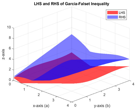
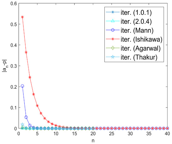
Take $\widetilde{s_n}={\displaystyle \frac{n}{n+1}}$ for all $n\in N$ and initial guess $a_0=2$. Numerical computations with MATLAB version 9.10.0.1602886 (R2021a) software suggest that $p\approx 1.25872$ is the unique fixed point of the map S, satisfying the fixed point equation $a=cos\left(a\right)+sin\left(a\right)$ approximately. Moreover, Figure 1 visually confirms that inequality (4) holds, indicating that the mapping S satisfies the $E_{\nu }$-property. Since S satisfies the Garcia-Falset property and $F\left(S\right)\ne \varnothing$, it follows from Theorem 3 that the iterative algorithm (1) converges to the fixed point $p\approx 1.25872$. Observe that the algorithm (1) converges faster than the iterative algorithms given by Picard–Mann, Mann, Ishikawa, and Thakur, as shown in

Table 1. Convergence behavior of $|a_n-p|$ for various iterative algorithms.

Numb. Iter.	Picard–Mann	Iter. (1)	Iter. (2)	Iter. Mann	Iter. Ishi.	Iter. Tha.
1	0.0161	9.5334 $\times {10}^{-4}$	3.852 $\times {10}^{-4}$	0.2031	0.5341	0.0188
2	0.0020	0	0	0.0834	0.3648	0.0022
3	2.6305 $\times {10}^{-4}$	0	0	0.0377	0.2450	2.5028 $\times {10}^{-4}$
4	0	0	0	0.0177	0.1636	0
5	0	0	0	0.0085	0.1089	0
6	0	0	0	0.0041	0.0723	0
7	0	0	0	0.0020	0.0480	0
8	0	0	0	9.8868 $\times {10}^{-4}$	0.0318	0
9	0	0	0	0	0.0210	0
10	0	0	0	0	0.0139	0
11	0	0	0	0	0.0092	0

and Figure 2.

In

Table 2. Convergence behavior at different initial points.

Initial Pts.	Picard–Mann	Iter. (1)	Iter. (2)	Iter. Mann	Iter. Ishi.	Iter. Tha.
0.1	6	4	3	13	21	6
1	4	3	2	9	16	4
3.5	5	3	2	11	20	5

, we compare the convergence of various iterative algorithms for different choices of initial points. The parameter $s_n$ was chosen to be ${\displaystyle \frac{2n}{5n+2}}$.

Example 3.

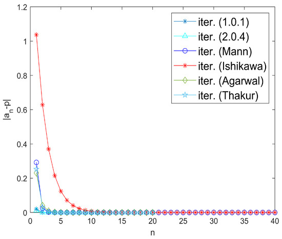
Let $A=[0,4]$ be endowed with the usual norm. Define a mapping $S:A\to A$ by $S\left(a\right)={\displaystyle \frac{1}{3}}+{\displaystyle \frac{1}{6}}cos\left(2a\right).$ Numerical simulations show that $p\approx 0.4396$ is a unique fixed point of S. Also, S satisfies $E_{\nu }$-property given by (4). Choose $\widetilde{s_n}={\displaystyle \frac{1}{n^2+1}},$ for all $n\in N$. We pick $a_0=2$ as initial guess. Now, all the conditions of Theorem 3 are fulfilled and iterative algorithm (1) converges to $p=0.4396.$ Clearly, it converges faster than the iterative algorithms given by Picard–Mann, Mann, Ishikawa, and Thakur, as shown in

Table 3. Convergence behavior of $|a_n-p|$ for various iterative algorithms.

Numb. Iter.	Picard–Mann	Iter. (1)	Iter. (2)	Iter. Mann	Iter. Ishi.	Iter. Tha.
1	0.2709	0.0316	0.0116	0.2921	1.0372	0.2530
2	0.0356	0.0013	2.1799 $\times {10}^{-4}$	0.0384	0.6288	0.0296
3	0.0051	6.7602 $\times {10}^{-5}$	0	0.0070	0.3703	0.036
4	7.3869 $\times {10}^{-4}$	0	0	0.0014	0.2151	4.3864 $\times {10}^{-4}$
5	0	0	0	3.1227 $\times {10}^{-4}$	0.1239	0
6	0	0	0	0	0.0709	0
7	0	0	0	0	0.0404	0
8	0	0	0	0	0.0230	0
9	0	0	0	0	0.0130	0
10	0	0	0	0	0.0073	0
11	0	0	0	0	0.0041	0

and Figure 3.

For parameter $s_n={\displaystyle \frac{2n}{5n+2}},$ 

Table 4. Convergence behavior at different initial points.

Initial Pts.	Picard–Mann	Iter. (1)	Iter. (2)	Iter. Mann	Iter. Ishi.	Iter. Tha.
0.1	5	3	2	5	12	4
1	5	3	3	5	13	5
3.5	4	3	2	7	20	5

exhibits the quicker convergence of the iterative algorithm (1) for different choices of initial points.

Example 4.

Suppose $A=[0,\infty )$ is equipped with the usual norm. Define the mapping $S:[0,\infty )\to [0,\infty )$ by:

$$\left\{\begin{array}{c}S\left(a\right)={\displaystyle \frac{a}{2}},a\ge 2\hfill \\ 0,a\in [0,2).\hfill \end{array}\right.$$

Note that S does not satisfy the Condition $\left(C\right)$. However, S is a Garcia-Falset mapping.

Indeed, for $a={\displaystyle \frac{3}{2}}$ and $b={\displaystyle \frac{5}{2}},$ we have

$${\displaystyle \frac{1}{2}}|a-S\left(a\right)|={\displaystyle \frac{1}{2}}|{\displaystyle \frac{3}{2}}-0|={\displaystyle \frac{3}{4}}.$$

Also

$$|a-b|=|{\displaystyle \frac{3}{2}}-{\displaystyle \frac{5}{2}}|=1.$$

Hence,

$${\displaystyle \frac{1}{2}}|a-S\left(a\right)|<|a-b|,$$

but $\left|S\right(a)-Sb|>|a-b|$. This implies that S does not satisfy the Condition $\left(C\right)$.

Suppose that $\nu =1$. Consider the following cases.

• Case I.
  $a>2$ and $b\in [0,2)$ give that

  $$\begin{array}{ccc}& & |a-Sb|\le \nu |a-Sa|+|a-b|\hfill \\ & & |a-0|\le |a-b|+|a-{\displaystyle \frac{a}{2}}|\hfill \\ & & \left|a\right|\le |a-b|+|{\displaystyle \frac{a}{2}}|\hfill \\ & & b\le {\displaystyle \frac{a}{2}},\hfill \end{array}$$

  which is true.
• Case II.
  When $a,b>2,$ it gives

  $$\begin{array}{ccc}& & |a-Sb|\le \nu |a-Sa|+|a-b|\hfill \\ & & |a-{\displaystyle \frac{b}{2}}|\le |a-b|+|a-{\displaystyle \frac{a}{2}}|\hfill \\ & & |{\displaystyle \frac{2a-b}{2}}|\le |a-b|+|{\displaystyle \frac{a}{2}}|\hfill \\ & & {\displaystyle \frac{2a-b}{2}}\le |a-b|+{\displaystyle \frac{a}{2}},\hfill \end{array}$$
  If $a<b$, we obtain $a-b\le 2(b-a)$, which leads to $a\le b$, a statement that is true. On the other hand, if $a\ge b$, we derive $a-b\ge 2(a-b)$, which simplifies to $0\ge a-b$, and this is also true.
• Case III.
  $a\in [0,2)$ and $b>2$ give

  $$\begin{array}{ccc}& & |a-Sb|\le \nu |a-Sa|+|a-b|\hfill \\ & & |a-{\displaystyle \frac{b}{2}}|\le |a-b|+|a-0|\hfill \\ & & |{\displaystyle \frac{2a-b}{2}}|\le |a-b|+|a|.\hfill \end{array}$$

We can easily check that it is true. Thus, S is the Garcia-Falset mapping.

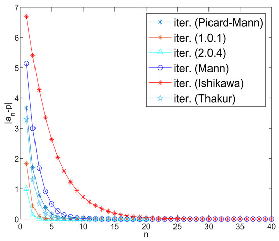
We now present a numerical experiment for the comparison of the convergence of algorithm (1). Taking an initial value $a_0=8\in A$ and $\widetilde{s_n}={\displaystyle \frac{n}{n^2+4n+1}}$, it is noted that the iterative algorithm (1) has the quickest convergence rate, as compared to other algorithms, as shown in

Table 5. Convergence behavior of $|a_n-p|$ for various iterative algorithms.

Numb. Iter.	Picard–Mann	Iter. (1)	Iter. (2)	Iter. Mann	Iter. Ishi.	Iter. Tha.
1	3.4286	1.8571429	1	4.571429	7.3878	3.676
2	1.4286	0.43112	0.12500	2.612245	6.8224	1.689475686151179
3	0.5882	0.1008	0.01563	1.47649	6.34841	0.7823
4	0.2406	0.02371	0.001953	0.8251	5.95301	0.365887450858190
5	0.09804	0.0056	2.441406 $\times {10}^{-4}$	0.4564	5.61952	0.172232522988864
6	0.0398	0.0013	0	0.250303	5.33445	0.081566
7	0.0161	3.18952 $\times {10}^{-4}$	0	0.13624	5.08764	0.038822964674253
8	0.00653	7.648328 $\times {10}^{-5}$	0	0.0737	4.87151	0.018557138861690
9	0.00264	1.839777 $\times {10}^{-5}$	0	0.039627	4.680323	0.008902166228661
10	0.00106	0	0	0.02121	4.50972	0.00428371
11	2103 $\times {10}^{-4}$	0	0	0.011303	4.356304	0.00206682
12	0	0	0	0.0060	4.2174	9.99533 $\times {10}^{-4}$
13	0	0	0	0.00317543	4.090894	4.843748124 $\times {10}^{-4}$
14	0	0	0	0.00167523	3.9750462	2.3515521 $\times {10}^{-4}$
15	0	0	0	8.8139084 $\times {10}^{-4}$	3.86845416	1.14348626 $\times {10}^{-4}$
16	0	0	0	4.6259333 $\times {10}^{-4}$	3.7699557	5.5685004 $\times {10}^{-5}$
17	0	0	0	2.4224943 $\times {10}^{-4}$	3.678581	0
18	0	0	0	1.26602718 $\times {10}^{-4}$	3.5935164	0
19	0	0	0	6.60410533 $\times {10}^{-5}$	3.5140696	0
20	0	0	0	0	3.439650976239416	0

and Figure 4 with fixed point 0.

Now, we compare the convergence of the iterative algorithm (1) with other iterative algorithms by choosing different initial points. Take parameter $s_n={\displaystyle \frac{2n}{5n+2}}$. Indeed, the algorithm (1) proves to be more suitable for Garcia-Falset operators as it has a quicker rate of convergence. The numerical results are demonstrated in

Table 6. Convergence behavior at different initial points.

Initial Pts.	Picard–Mann	Iter. (1)	Iter. (2)	Iter. Mann	Iter. Ishi.	Iter. Tha.
8	12	8	6	-	-	13
2	10	7	5	29	-	12
10	12	8	6	34	-	13
40	13	9	7	37	-	13
1	9	1	1	9	26	1

.

In the following example, it must be noted that the mapping does not have a unique fixed point, and different iterative processes may converge to any of the fixed points for a certain initial value. Hence, to test the convergence, we employ an appropriate stopping criterion: $\parallel a_n-a_{n-1}\parallel +\parallel b_n-b_{n-1}\parallel \le 0.005$ for $n\in \mathbb{N}$, $(a_n,b_n)\in {\mathbb{R}}^2.$

Example 5.

Define a mapping $S:{[0,2]}^2\to {[0,2]}^2$ by,

$$Sa=\left\{\begin{array}{c}({\displaystyle \frac{1}{7}}{(a_1+{\displaystyle \frac{1}{2}})}^2,2-{\displaystyle \frac{2}{5}}{a}_2),a_1\in [0,{\displaystyle \frac{1}{5}})\hfill \\ ({\displaystyle \frac{a_1}{5}}+{\displaystyle \frac{2}{5}},2-{\displaystyle \frac{2}{5}}{a}_2),a_1\in [{\displaystyle \frac{1}{5}},2].\hfill \end{array}\right.$$

where $a=(a_1,a_2)$. The distance between the points is defined using the Euclidean norm. First, we show that S is not non-expansive. Consider the points $a=(0.1,0.5)$ and $b=(0.3,0.5)$. Then,

$$S\left(a\right)=\left({\displaystyle \frac{1}{7}}{\left(0.6\right)}^2,1.8\right)\approx (0.0514,1.8),S\left(b\right)=\left(0.46,1.8\right).$$

We compute the Euclidean distance:

$$\parallel S\left(a\right)-S\left(b\right)\parallel =\sqrt{{(0.0514-0.46)}^2+{(1.8-1.8)}^2}=0.4086,$$

and

$$\parallel a-b\parallel =\sqrt{{(0.1-0.3)}^2+{(0.5-0.5)}^2}=0.2.$$

Thus,

$$\parallel S\left(a\right)-S\left(b\right)\parallel \approx 0.4086,\parallel a-b\parallel =0.2,$$

which implies $\parallel S\left(a\right)-S\left(b\right)\parallel >\parallel a-b\parallel$. Hence, S is not non-expansive.

To show that S satisfies the Garcia-Falset property, we consider the following cases:

• Case I.
  If $a_1,b_1\in [0,{\displaystyle \frac{1}{5}}),$ then for $\nu =1$, following inequality, it must hold for S to satisfy the condition $\left(E_1\right)$

  $$\begin{array}{ccc}& & |a_1-{\displaystyle \frac{1}{7}}{b}_1-{\displaystyle \frac{1}{7}}{b_1}^2-{\displaystyle \frac{1}{28}}|+|a_2-{\displaystyle \frac{2}{5}}{b}_2-2|\hfill \\ & \le & |a_1-{\displaystyle \frac{1}{7}}(a_1+{\displaystyle \frac{1}{2}}){|}^2+|a_2-2+{\displaystyle \frac{2}{5}}{a}_2|+|a_1-b_1|+|a_2-b_2|.\hfill \end{array}$$
  Divide the above inequality into two parts:

  $$\begin{array}{ccc}\hfill |a_1-{\displaystyle \frac{1}{7}}{b}_1-{\displaystyle \frac{1}{7}}{b_1}^2-{\displaystyle \frac{1}{28}}|& \le & |a_1-{\displaystyle \frac{1}{7}}(a_1+{\displaystyle \frac{1}{2}}){|}^2+|a_1-b_1|.\hfill \end{array}$$

  (22)

  $$\begin{array}{ccc}\hfill |a_2+{\displaystyle \frac{2}{5}}{b}_2-2|& \le & |a_2-2+{\displaystyle \frac{2}{5}}{a}_2|+|a_2-b_2|.\hfill \end{array}$$

  (23)

  If we consider (22), then for $a_1,b_1\in [0,{\displaystyle \frac{1}{5}})$, we have

  $$|a_1-{\displaystyle \frac{1}{7}}{b}_1-{\displaystyle \frac{1}{7}}{b_1}^2-{\displaystyle \frac{1}{28}}|\le {\displaystyle \frac{23}{140}}$$

  and

  $$|a_1-{\displaystyle \frac{1}{7}}(a_1+{\displaystyle \frac{1}{2}}){|}^2+|a_1-b_1|\le {\displaystyle \frac{395}{196}}\ge {\displaystyle \frac{23}{140}}.$$

  If we take (23), then for the given range of $a_2$ and $b_2$, we have

  $$|a_2-{\displaystyle \frac{2}{5}}{b}_2-2|\le 2$$

  and

  $$|a_2-2+{\displaystyle \frac{2}{5}}{a}_2|+|a_2-b_2|\le 4\ge 2.$$

  From the above inequalities, it is clear that S has the Garcia-Falset property.
• Case II.
  Let $a_1,b_1\in [{\displaystyle \frac{1}{5}},2],$ then for $\nu =1$, following inequality, it should hold for S to satisfy the condition $\left(E_1\right);$

  $$\begin{array}{ccc}& & |a_1-{\displaystyle \frac{1}{5}}{b}_1-{\displaystyle \frac{2}{5}}|+|a_2+{\displaystyle \frac{2}{5}}{b}_2-2|\hfill \\ & \le & |a_1-{\displaystyle \frac{1}{5}}(a_1+2)|+|a_2-2+{\displaystyle \frac{2}{5}}{a}_2|+|a_1-b_1|+|a_2-b_2|.\hfill \end{array}$$

Again, divide the above inequality into two parts:

$$\begin{array}{ccc}\hfill |a_1-{\displaystyle \frac{1}{5}}{b}_1-{\displaystyle \frac{2}{5}}|& \le & |a_1-{\displaystyle \frac{1}{5}}(a_1+2)|+|a_1-b_1|.\hfill \end{array}$$

(24)

$$\begin{array}{ccc}\hfill |a_2+{\displaystyle \frac{2}{5}}{b}_2-2|& \le & |a_2-2+{\displaystyle \frac{2}{5}}{a}_2|+|a_2-b_2|.\hfill \end{array}$$

(25)

For the given range of a and b, (24) becomes

$$\begin{array}{cc}\hfill |a_1-{\displaystyle \frac{1}{5}}{b}_1-{\displaystyle \frac{2}{5}}|& \le 1.56.\\ \hfill |a_1-{\displaystyle \frac{1}{5}}(a_1+2)|+|a_1-b_1|& \le 3.\end{array}$$

That is, $1.56<3.$ So the inequality is satisfied. The inequality (25) is proven in Case I. Hence, S satisfies the Garcia-Falset property for Case II.

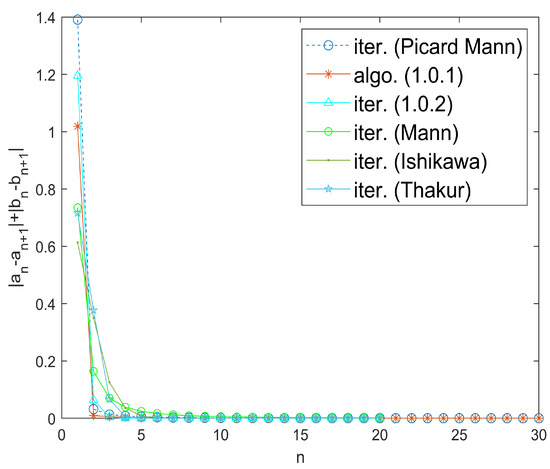
To analyze the rate of convergence of different iterative algorithms and iterative algorithm (1), we have chosen the sequence $\widetilde{s_n}=\sqrt{{\displaystyle \frac{n}{n+1}}}$ with initial guess as $(a_0,b_0)=(0.25,0.5)$. Finally, through numerical approximation using MATLAB version 9.10.0.1602886 (R2021a) software, it is determined that the iterative algorithm (1) converges to the fixed point $({\displaystyle \frac{1}{2}},{\displaystyle \frac{10}{7}})$ faster than Picard–Mann, Mann, Ishikawa, and Thakur’s iterative algorithms, as shown in Figure 5.

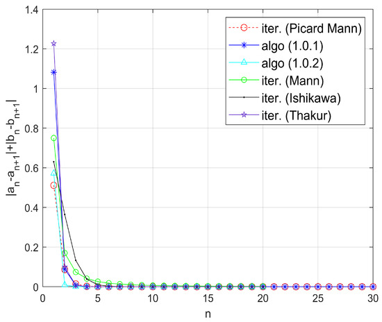
Again, for a different initial guess $(1,1.5),$ we conclude that the iterative algorithm (1) converges to fixed point $(0.04,{\displaystyle \frac{10}{7}})$ faster than Picard–Mann, Mann, Ishikawa, and Thakur iterative algorithms, as shown in Figure 6.

Now, we compare the iterative algorithms using different initial points. It can be observed from

Table 7. Convergence behavior at different initial points.

Initial Pts.	Picard–Mann	Iter. (1)	Iter. (2)	Iter. Mann	Iter. Ishi.	Iter. Tha.
(0.25, 0.5)	5	3	3	10	6	5
(1, 1.5)	4	3	3	-	6	12
(0.5,1.3)	5	3	3	4	4	4
(0.1,1.9)	6	4	4	8	5	4

that algorithm (1) and its Case (2) converges in a lesser number of iterations.

6. Application to Volterra–Stieltjes-Type Delay Functional Differential Equation

Recently, many authors have studied the existence and uniqueness of the solution of Volterra–Stieltjes-type delay functional differential equations, see [27,28] and references therein. As an application of our results, we propose the approximation of the weak solution of Volterra–Stieltjes-type delay functional differential equation utilizing the iterative method (1). Suppose B is a reflexive Banach space equipped with the norm ${\parallel .\parallel }_B$, the dual space of B is denoted as $B^{*}$, and the class of continuous functions is denoted as $\mathcal{C}[L,B],$$L=[0,I]$ with the norm as follows:

$${\parallel a\parallel }_{\mathcal{C}}=\underset{i\in L}{sup}{\parallel a\left(i\right)\parallel }_B,a\in \mathcal{C}[L,B].$$

Let us consider a non-linear second-order Volterra–Stieltjes-type initial value delay functional differential problem as follows:

$${\displaystyle \frac{d}{di}}a\left(i\right)=g_1\left(i,{\int }_0^{h\left(i\right)}{g}_2(i,s,a\left(s\right))d_{s}f(i,s)\right),i\in L$$

(26)

with the initial condition

$$a\left(0\right)=a_0.$$

(27)

Let us consider the following assumptions:

i.

$h:L\to L$ is continuously non-decreasing and $h\left(i\right)\le i.$

ii.

For $q=1,2$, each $g_q:L\times B\to B$ weakly fulfills the Lipschitz condition and is weakly continuous, such that

$$|\varphi (g_q(i,a)-g_q(i,b))|\le k_q\left|\varphi (a-b)\right|,k_q>0,\forall (i,a),(i,b)\in L\times B,\varphi \in B^{*}.$$

where $k_q$ are Lipschitz constants.

iii

$f:L\times \mathbb{R}\to \mathbb{R}$ is continuous function with

$$m=max\{sup|f(i,h(i\left)\right)|+sup|f(i,0)\left|\right\}\mathrm{on}L.$$

iv.

$k_1{k}_{2}mi<1.$

Lemma 5

([27]). A solution of the non-linear second-order Volterra–Stieltjes-type initial value delay functional differential problem (26) and (27) exists whenever it is expressed as an integral equation as follows:

$$a\left(i\right)=a_0+{\int }_0^i{g}_1\left(t,{\int }_0^{h\left(i\right)}{g}_2(t,\theta ,a\left(\theta \right))\right)d_{\theta }f(t,\theta )dt.$$

We derive the following theorem for the existence of the solution of (26) and (27) by using an iterative algorithm (1).

Theorem 7.

Suppose that the assumptions (i)–(iv) hold and $\left\{a_n\right\}$ is a sequence approximated by (1). Then, initial value problem (26) and (27) has a unique solution $p\in \mathcal{C}[L,B]$ and $a_n$ converges to $p.$

Proof. 

Let $\left\{a_n\right\}$ be sequence approximated by (1). Let S be an operator on $\mathcal{C}[L,B]$ by

$$S\left(a\left(i\right)\right)=a_0+{\int }_0^i{g}_1\left(t,{\int }_0^{h\left(i\right)}{g}_2(t,\theta ,a\left(\theta \right))\right)d_{\theta }f(t,\theta )dt.$$

We have

$$\begin{array}{ccc}\hfill \parallel c_n{-p\parallel }_{\mathcal{C}}& =& \parallel (1-\widetilde{s_n})S{a}_n+\widetilde{s_n}{S}^2{a}_n{-p\parallel }_{\mathcal{C}}\hfill \\ & \le & (1-\widetilde{s_n})\parallel S{a}_n-p\parallel +|\widetilde{s_n}{\parallel S^2{a}_n-p\parallel }_{\mathcal{C}}.\hfill \end{array}$$

(28)

Consider

$$\begin{array}{ccc}\hfill \parallel S{a}_n{-p\parallel }_{\mathcal{C}}& =& \parallel S{a}_n-Sp\parallel \hfill \\ & \le & \parallel a_0+{\int }_0^i{g}_1\left(t,{\int }_0^{h\left(t\right)}{g}_2(t,\theta ,a_n\left(\theta \right))\right)d_{\theta }f(t,\theta )dt-\hfill \\ & & a_0-{\int }_0^i{g}_1\left(t,{\int }_0^{h\left(t\right)}{g}_2(t,\theta ,p\left(\theta \right))\right)d_{\theta }f(t,\theta )dt{\parallel }_{\mathcal{C}}\hfill \\ & =& \left|S\right({\int }_0^i{g}_1\left(t,{\int }_0^{h\left(t\right)}{g}_2(t,\theta ,a_n\left(\theta \right))\right)d_{\theta }f(t,\theta )dt-\hfill \\ & & {\int }_0^i{g}_1\left(t,{\int }_0^{h\left(t\right)}{g}_2(t,\theta ,p\left(\theta \right))\right)d_{\theta }f(t,\theta )\left)dt\right|.\hfill \end{array}$$

Using assumption (ii), we have

$$\begin{array}{ccc}\hfill \parallel S{a}_n{-p\parallel }_{\mathcal{C}}& \le & {\int }_0^i{k}_1\left|S\right({\int }_0^{h\left(t\right)}{g}_2(t,\theta ,a_n\left(\theta \right)))d_{\theta }f(t,\theta )-\hfill \\ & & {\int }_0^{h\left(t\right)}{g}_2(t,\theta ,p\left(\theta \right))d_{\theta }f(t,\theta )\left)\right|dt\hfill \\ & \le & k_1{\int }_0^i{\int }_0^{h\left(t\right)}\left|S\right(g_2(t,\theta ,a_n\left(\theta \right)))-\hfill \\ & & g_2(t,\theta ,p\left(\theta \right))\left)d_{\theta }f(t,\theta )\right|dt,\hfill \end{array}$$

and

$$\begin{array}{ccc}\hfill \parallel S{a}_n{-p\parallel }_{\mathcal{C}}& \le & k_1{\int }_0^i{\int }_0^{h\left(t\right)}{k}_2\left|S\left(a_n\left(\theta \right)-p\left(\theta \right)\right)d_{\theta }f(t,\theta )\right|dt\hfill \\ & \le & k_1{k}_2{\parallel a_n-p\parallel }_{\mathcal{C}}{\int }_0^i{\int }_0^{h\left(t\right)}{d}_{\theta }f(t,\theta )dt\hfill \\ & =& k_1{k}_2{\parallel a_n-p\parallel }_{\mathcal{C}}{\int }_0^i(f(t,h\left(t\right))-f(t,0))dt\hfill \\ & \le & k_1{k}_{2}m{\parallel a_n-p\parallel }_{\mathcal{C}}{\int }_0^{i}dt\hfill \\ & =& k_1{k}_{2}mi{\parallel a_n-p\parallel }_{\mathcal{C}}.\hfill \end{array}$$

Moreover, $k_1{k}_{2}mi<1$ yields

$$\begin{array}{ccc}\hfill \parallel S{a}_n{-p\parallel }_{\mathcal{C}}& \le & \parallel a_n{-p\parallel }_{\mathcal{C}}.\hfill \end{array}$$

(29)

Also,

$$\begin{array}{ccc}\hfill \parallel S^2{a}_n{-p\parallel }_{\mathcal{C}}& =& \parallel S\left(S{a}_n\right)-Sp\parallel \hfill \\ & =& \parallel a_0+{\int }_0^i{g}_1\left(t,{\int }_0^{h\left(t\right)}{g}_2(t,\theta ,S{a}_n\left(\theta \right))\right)d_{\theta }f(t,\theta )dt-\hfill \\ & & a_0-{\int }_0^i{g}_1\left(t,{\int }_0^{h\left(t\right)}{g}_2(t,\theta ,p\left(\theta \right))\right)d_{\theta }f(t,\theta )dt{\parallel }_{\mathcal{C}}\hfill \\ & =& \left|S\right({\int }_0^i{g}_1\left(t,{\int }_0^{h\left(t\right)}{g}_2(t,\theta ,S{a}_n\left(\theta \right))\right)d_{\theta }f(t,\theta )dt-\hfill \\ & & {\int }_0^i{g}_1\left(t,{\int }_0^{h\left(t\right)}{g}_2(t,\theta ,p\left(\theta \right))\right)d_{\theta }f(t,\theta )\left)dt\right|.\hfill \end{array}$$

Further, from assumption (ii), we get

$$\begin{array}{ccc}\hfill \parallel S^2{a}_n{-p\parallel }_{\mathcal{C}}& \le & {\int }_0^i{k}_1\left|S\right({\int }_0^{h\left(t\right)}{g}_2(t,\theta ,S{a}_n\left(\theta \right)))d_{\theta }f(t,\theta )-\hfill \\ & & {\int }_0^{h\left(t\right)}{g}_2(t,\theta ,p\left(\theta \right))d_{\theta }f(t,\theta )\left)\right|dt\hfill \\ & \le & k_1{\int }_0^i{\int }_0^{h\left(t\right)}\left|S\right(g_2(t,\theta ,S{a}_n\left(\theta \right)))-\hfill \\ & & g_2(t,\theta ,p\left(\theta \right))\left)d_{\theta }f(t,\theta )\right|dt,\hfill \end{array}$$

and

$$\begin{array}{ccc}\hfill \parallel S^2{a}_n{-p\parallel }_{\mathcal{C}}& \le & k_1{\int }_0^i{\int }_0^{h\left(t\right)}{k}_2\left|S\left(S{a}_n\left(\theta \right)-p\left(\theta \right)\right)d_{\theta }f(t,\theta )\right|dt\hfill \\ & \le & k_1{k}_2{\parallel S{a}_n-p\parallel }_{\mathcal{C}}{\int }_0^i{\int }_0^{h\left(t\right)}{d}_{\theta }f(t,\theta )dt\hfill \\ & =& k_1{k}_2{\parallel S{a}_n-p\parallel }_{\mathcal{C}}{\int }_0^i(f(t,h\left(t\right))-f(t,0))dt\hfill \\ & \le & k_1{k}_{2}m{\parallel S{a}_n-p\parallel }_{\mathcal{C}}{\int }_0^{i}dt\hfill \\ & =& k_1{k}_{2}mi{\parallel S{a}_n-p\parallel }_{\mathcal{C}}.\hfill \end{array}$$

Since $k_1{k}_{2}mi<1$,

$$\begin{array}{ccc}\hfill \parallel S^2{a}_n{-p\parallel }_{\mathcal{C}}& \le & \parallel S{a}_n{-p\parallel }_{\mathcal{C}}.\hfill \end{array}$$

Using (29) we obtain

$$\begin{array}{ccc}\hfill \parallel S^2{a}_n{-p\parallel }_{\mathcal{C}}& \le & \parallel a_n{-p\parallel }_{\mathcal{C}}.\hfill \end{array}$$

We have

$$\begin{array}{ccc}\hfill \parallel c_n-p\parallel & \le & (1-\widetilde{s_n})\parallel a_n-p\parallel +|\widetilde{s_n}{\parallel a_n-p\parallel }_{\mathcal{C}}\hfill \\ & \le & \parallel a_n{-p\parallel }_{\mathcal{C}}.\hfill \end{array}$$

(30)

Thus,

$$\begin{array}{ccc}\hfill \parallel b_n-p\parallel & =& \parallel S{c}_n-p\parallel \hfill \\ & \le & \parallel a_n-p\parallel .\hfill \end{array}$$

By setting $\parallel a_n{-p\parallel }_{\mathcal{C}}=r_n,$ we obtain

$$r_{n+1}\le r_n,\mathrm{for}\mathrm{all}n\in \mathbb{N},$$

which implies

$$\underset{n\to \infty }{lim}{r}_n=0.$$

So, $a_n\to p.$ □

7. Conclusions

In this paper, an iterative algorithm (1) is analyzed for generalized non-expansive mappings satisfying the Garcia-Falset property on a uniformly convex Banach space. Weak and strong convergence theorems for such mappings are established. It is demonstrated that the iterative algorithm (1) is ${\omega }^2$-stable. Numerical experiments have been performed to show that this iterative algorithm converges to a fixed point faster than iterative algorithms such as Picard–Mann, Mann, Ishikawa, and Thakur. To exhibit the utility of the proposed results, we approximated the weak solution of Volterra–Stieltjes-type delay functional differential equation using the mentioned iterative algorithm.

References

- Berinde, V.; Takens, F. Iterative Approximation of Fixed Points; Springer: Berlin/Heidelberg, Germany, 2007; Volume 1912. [Google Scholar]
- Kirk, W.A. A fixed point theorem for mappings that do not increase distances. Am. Math. Mon. 1965, 72, 1004–1006. [Google Scholar] [CrossRef]
- Browder, F.E. Nonexpansive nonlinear operators in a Banach space. Proc. Natl. Acad. Sci. USA 1965, 54, 1041–1044. [Google Scholar] [CrossRef]
- Göhde, D. Zum Prinzip der Kontraktiven Abbildung. Math. Nachr. 1965, 30, 251–258. [Google Scholar] [CrossRef]
- Krasnoselskii, M.A. Two remarks on the method of successive approximations. Uspekhi Math. Nauk. 1955, 10, 123–127. [Google Scholar]
- Mann, W.R. Mean value methods in iteration. Proc. Am. Math. Soc. 1953, 4, 506–510. [Google Scholar] [CrossRef]
- Ishikawa, S. Fixed points by a new iteration method. Proc. Am. Math. Soc. 1974, 44, 147–150. [Google Scholar] [CrossRef]
- Abbas, M.; Nazir, T. A new, faster iteration process applied to constrained minimization and feasibility problems. Mat. Vesn. 2014, 66, 223–234. [Google Scholar]
- Thakur, B.S.; Thakur, D.; Postolache, M. A new iterative scheme for numerical reckoning fixed points of Suzuki’s generalized nonexpansive mappings. Appl. Math. Comput. 2016, 275, 147–155. [Google Scholar] [CrossRef]
- Khan, S.H. A Picard-Mann hybrid iterative process. Fixed Point Theory Appl. 2013, 2013, 69. [Google Scholar] [CrossRef]
- Suzuki, T. Fixed point theorems and convergence theorems for some generalized nonexpansive mappings. J. Math. Anal. Appl. 2008, 340, 1088–1095. [Google Scholar] [CrossRef]
- Garcia-Falset, J.; Llorens-Fuster, E.; Suzuki, T. Fixed point theory for a class of generalized nonexpansive mappings. J. Math. Anal. Appl. 2011, 375, 185–195. [Google Scholar] [CrossRef]
- Usurelu, G.I.; Postolache, M. Convergence analysis for a three-step Thakur iteration for Suzuki-type nonexpansive mappings with visualization. Symmetry 2019, 11, 1441. [Google Scholar] [CrossRef]
- Houmani, H.; Turcanu, T. CQ-Type algorithm for reckoning best proximity points of EP-operators. Symmetry 2019, 12, 4. [Google Scholar] [CrossRef]
- Maldar, S.; Gürsoy, F.; Atalan, Y.; Abbas, M. On a three-step iteration process for multivalued Reich-Suzuki type α-nonexpansive and contractive mappings. J. Appl. Math. Comput. 2022, 68, 863–883. [Google Scholar] [CrossRef]
- Pant, R.; Shukla, R. Approximating fixed points of generalized α-nonexpansive mappings in Banach spaces. Numer. Anal. Optim. 2017, 38, 248–266. [Google Scholar] [CrossRef]
- Gürsoy, F.; Khan, A.R.; Ertürk, M.; Karakaya, V. Weak w2 and data dependence of Mann iteration method in Hilbert spaces. Rev. Real Acad. Cienc. Exactas Fís. Nat. Ser. A Mat. 2019, 113, 11–20. [Google Scholar] [CrossRef]
- Hacıoğlu, E.; Gürsoy, F.; Maldar, S.; Atalan, Y.; Milovanović, G.V. Iterative approximation of fixed points and applications to two-point second-order boundary value problems and to machine learning. Appl. Numer. Math. 2021, 167, 143–172. [Google Scholar] [CrossRef]
- Khatoon, S.; Uddin, I.; Ali, J.; George, R. Common fixed points of two nonexpansive mappings via a faster iteration procedure. J. Funct. Spaces 2021, 2021, 9913540. [Google Scholar] [CrossRef]
- Maniu, G. On a three-step iteration process for Suzuki mappings with a qualitative study. Numer. Funct. Anal. Optim. 2020, 41, 929–949. [Google Scholar] [CrossRef]
- Hacıoğlu, E. A comparative study on iterative algorithms of almost contractions in the context of convergence, stability, and data dependency. Comput. Appl. Math. 2021, 40, 282. [Google Scholar] [CrossRef]
- Timis, I. On the weak stability of Picard iteration for some contractive type mappings. Ann. Univ. Craiova Math. Comput. Sci. Ser. 2010, 37, 106–114. [Google Scholar]
- Senter, H.F.; Dotson, W. Approximating fixed points of nonexpansive mappings. Proc. Am. Math. 1974, 44, 375–380. [Google Scholar] [CrossRef]
- Edelstein, M. Fixed point theorems in uniformly convex Banach spaces. Proc. Am. Math. Soc. 1974, 44, 369–374. [Google Scholar] [CrossRef]
- Clarkson, J.A. Uniformly convex spaces. Trans. Am. Math. Soc. 1936, 40, 396–414. [Google Scholar] [CrossRef]
- Schu, J. Weak and strong convergence to fixed points of asymptotically nonexpansive mappings. Bull. Aust. Math. Soc. 1991, 43, 153–159. [Google Scholar] [CrossRef]
- El-Sayed, A.M.; Omar, Y.M. On the weak solutions of a delay composite functional integral equation of Volterra-Stieltjes type in reflexive Banach space. Mathematics 2022, 10, 245. [Google Scholar] [CrossRef]
- Beg, I.; Abbas, M.; Asghar, M.W. Convergence of AA-Iterative Algorithm for Generalized α-Nonexpansive Mappings with an Application. Mathematics 2022, 10, 4375. [Google Scholar] [CrossRef]
Disclaimer/Publisher’s Note: The statements, opinions and data contained in all publications are solely those of the individual author(s) and contributor(s) and not of MDPI and/or the editor(s). MDPI and/or the editor(s) disclaim responsibility for any injury to people or property resulting from any ideas, methods, instructions or products referred to in the content. |
© 2025 by the authors. Licensee MDPI, Basel, Switzerland. This article is an open access article distributed under the terms and conditions of the Creative Commons Attribution (CC BY) license (https://creativecommons.org/licenses/by/4.0/).