Numerical Simulations for Parabolic Stochastic Equations Using a Structure-Preserving Local Discontinuous Galerkin Method

Abstract

In this paper, a structure-preserving local discontinuous Galerkin (LDG) method is proposed for parabolic stochastic partial differential equations with periodic boundary conditions and multiplicative noise. It is proven that under certain conditions, this numerical method is stable in the $L^2$ sense and can preserve energy conservation. The optimal spatial error estimate in the mean square sense can reach $n+1$ if the degree of the polynomial is n. The correctness of the theoretical results is verified through numerical examples.

1. Introduction

Partial differential equations (PDEs) have a wide range of applications in many fields, from physics and engineering to biology and finance. These equations play a fundamental role in the modeling of complex phenomena [1,2]. However, in nature, many phenomena are affected by stochastic factors. Stochastic differential equations can better describe these random factors in natural processes. Due to the complexity of many real-world problems, it is often difficult, even near impossible, to obtain analytical solutions to partial differential equations. Therefore, numerical methods for partial differential equations have received great attention from scholars [3,4,5,6,7,8,9,10,11,12]. Parabolic equations are widely used to describe diffusion processes, heat conduction phenomena, and problems such as option pricing in financial mathematics. Classical parabolic equations are typically employed to describe diffusion behaviors in deterministic systems, while stochastic parabolic equations, by introducing stochastic terms, can more accurately model complex systems in the real world that are subject to noise interference. With the development of stochastic analysis theory and numerical methods, significant progress has been made in the study of stochastic parabolic equations. Numerical methods for solving stochastic partial differential equations mainly include finite difference methods, finite element methods, discontinuous Galerkin (DG) methods, and so on [13,14,15,16,17].

The DG method, because of its flexibility and high accuracy, exhibits significant advantages when dealing with high-order derivatives and complex boundary conditions. The LDG method overcomes the limitations of traditional DG methods in handling high-order derivatives by introducing auxiliary variables to transform high-order equations into first-order systems. Yan and Shu [18] used the LDG method to propose appropriate numerical fluxes for general KdV-type equations with third-order derivatives, time-dependent biharmonic equations with fourth-order derivatives, and partial differential equations with fifth-order derivatives, which proves stability for most nonlinear problems. Chen [19] proposed the symplectic LDG method for stochastic linear Schrödinger equations with multiplicative noise and concluded that the mean-square error is bounded by the time and space step sizes and their ratios. Li [20] developed an LDG method for solving backward stochastic partial differential equations, proving the stability of the numerical scheme, obtaining optimal error estimates on Cartesian meshes, and deriving suboptimal error estimates on triangular meshes. Li [21] introduced the LDG method for solving multidimensional nonlinear second-order partial differential equations and applied the proposed method to stochastic optimal control problems. Wang [22] proposed two fully discrete IMEX-LDG schemes by combining the LDG spatial discretization with the implicit–explicit Runge–Kutta temporal discretization and performed stability and error analysis for the linearized KdV equation.

From the above literature, it is evident that the LDG method, due to its stability and high accuracy, demonstrates significant advantages in handling high-order equations. Although the LDG method has been successfully applied to various deterministic problems, its application to stochastic equations remains limited. Therefore, this paper discusses the LDG method for stochastic linear parabolic equations and explores whether the numerical solutions obtained by this method can preserve the long-term behavior of the original systems.

Zhang [23] provided sufficient conditions for stochastic multi-symplectic conservation of stochastic Runge–Kutta methods for stochastic Hamiltonian partial differential equations. Zhou [24] proposed a second-order fractional difference-based Crank–Nicholson discretization to ensure the conservation of the energy-preserving or energy-dissipating properties in stochastic space-fractional nonlinear wave equations under appropriate conditions. Hou [25] derived an energy-preserving semidiscretization scheme that preserves symplectic structures to solve stochastic Maxwell equations and proposed two fully discrete symplectic-preserving, multi-symplectic-preserving and energy-preserving methods. Bai [26] presented a high-order mass-conserving and energy-conserving method for solving nonlinear Schrödinger equations, proving the existence, uniqueness, and high-order convergence of numerical solutions.

In this paper, the following parabolic stochastic partial differential equations (SPDEs) driven by multiplicative noise with a periodic boundary condition are considered

$$\left\{\begin{array}{c}\mathrm{d}u(x,t)=\left(a{u}_{xx}(x,t)+b{u}_x(x,t)+cu(x,t)\right)\mathrm{d}t+\left(\alpha u_x(x,t)+\beta u(x,t)\right)\mathrm{d}{W}_t,\hfill \\ u(x,0)=u_0\left(x\right),\hfill \end{array}\right.$$

(1)

where $(x,t)\in [0,l]\times [0,T]$ and $I=[0,l]$. $a\ne 0$, b, c, $\alpha$, and $\beta$ are constants. $\left\{W_t,0\le t\le T\right\}$ is a standard one-dimensional Brownian motion, which is a real-valued continuous $\left\{{\mathcal{F}}_t\right\}$ adapted process on a complete probability space $(\Omega ,\mathcal{F},\mathbb{P})$. Some of the properties of Brownian motion and stochastic integral are summarized below [27]:

(1)

For $0\le s<t<\infty$, the increment $W_t-W_s$ is normally distributed with mean zero and variance $t-s$.

(2)

$\left\{W_t\right\}$ is a continuous square-integrable martingale and its quadratic variation ${⟨W,W⟩}_t=t$ for all $t\ge 0$.

(3)

Let $f\in {\mathcal{M}}^2([a_1,b_1];R)$, the family of $R^d$-valued ${\mathcal{F}}_t$-adapted processes such that ${\int }_{a_1}^{b_1}{\left|f\left(t\right)\right|}^{p}dt<\infty a.s.$ and mathematical expectation $E{\int }_{a_1}^{b_1}{\left|f\left(t\right)\right|}^{p}dt<\infty$, then ${\int }_{a_1}^{b_1}f\left(t\right)d{W}_t$ is ${\mathcal{F}}_{b_1}$-measurable and $E{\int }_{a_1}^{b_1}f\left(t\right)d{W}_t=0$.

In this paper a structure-preserving LDG method is proposed for parabolic SPDEs (1). The rest of this paper is organized as follows. In Section 2, we introduce some preliminary knowledge, notations, and definitions. The numerical scheme of the LDG methods is presented in Section 3. The stability and energy preservation properties of the LDG method is analyzed in Section 4. The optimal error estimation of the proposed method is considered in Section 5. In Section 6, numerical experiments are conducted to validate the theoretical results.

2. Preliminaries

In this section, some preliminary knowledge used in the article is introduced, including notations, definitions, and some lemmas.

Denote the regular spatial mesh by $I_j=\left[x_{j-\frac{1}{2}},x_{j+\frac{1}{2}}\right]$, $j=1,\dots ,N$ with the center of the cell denoted by $x_j=\frac{1}{2}(x_{j-\frac{1}{2}}+x_{j+\frac{1}{2}})$. Here, $x_{\frac{1}{2}}=0$ and $x_{N+\frac{1}{2}}=l$, $h_j=x_{j+\frac{1}{2}}-x_{j-\frac{1}{2}}$, with $h=\underset{1\le j\le N}{max}{h}_j$ denoting the mesh size.

Through out this paper, the Sobolev space $H^{m,p}$ with periodic boundary conditions is considered

$$\begin{array}{cc}\hfill H^{m,p}:=\left\{u\left(x\right),x\in (0,l)\mid {\parallel u\parallel }_{H^{m,p}}=\right.& {\left[{\int }_0^l\left({\left|u\left(x\right)\right|}^p+{\displaystyle \sum _{k=1}^m}{\left|{\displaystyle \frac{{\mathrm{d}}^{k}u\left(x\right)}{\mathrm{d}{x}^k}}\right|}^p\right)\mathrm{d}x\right]}^{{\displaystyle \frac{1}{p}}}<\infty \hfill \\ \hfill & \left.{\displaystyle \frac{{\mathrm{d}}^{k}u\left(0\right)}{\mathrm{d}{x}^k}}={\displaystyle \frac{{\mathrm{d}}^{k}u\left(l\right)}{\mathrm{d}{x}^k}},k=0,1,\dots ,m-1\right\}.\hfill \end{array}$$

We denote $L^2(0,l)$ space with norm $\parallel ·\parallel$ as $L^2$, Sobolev space $H^{m,p}(0,l)$ with norm ${\parallel ·\parallel }_{H^{m,p}}$ as $H^{m,p}$, specially, norm ${\parallel ·\parallel }_{H^{m,2}}$ as ${\parallel ·\parallel }_{H^m}$.

The following lemma is the multidimensional Itô formula for continuous and square integrable martingales.

Lemma 1

([28]). Suppose $M_1\left(t\right),\dots ,M_n\left(t\right)$ are continuous, square integrable martingales. Let $F\left(t,x_1,\dots ,x_n\right)$ be a continuous function with continuous partial derivatives ${\displaystyle \frac{\partial F}{\partial t}},{\displaystyle \frac{\partial F}{\partial x_i}}$, and ${\displaystyle \frac{{\partial }^{2}F}{\partial x_i\partial x_j}}$ for $1\le i,j\le n$. Then, we know

$$\mathrm{d}F={\displaystyle \frac{\partial F}{\partial t}}\mathrm{d}t+{\displaystyle \sum _{i=1}^n}{\displaystyle \frac{\partial F}{\partial x_i}}\mathrm{d}{M}_i\left(t\right)+\frac{1}{2}{\displaystyle \sum _{i,j=1}^n}{\displaystyle \frac{{\partial }^{2}F}{\partial x_i\partial x_j}}\mathrm{d}{⟨M_i,M_j⟩}_t,$$

where ${⟨·,·⟩}_t$ is the cross variation process.

By the Itô formula, for continuous semi-martingales X and Y, we have

$$X_t{Y}_t=X_0{Y}_0+{\int }_0^t{X}_s\mathrm{d}{Y}_s+{\int }_0^t{Y}_s\mathrm{d}{X}_s+{⟨X,Y⟩}_t.$$

(2)

For any locally bounded adapted process H, we have

$${⟨{\int }_0{H}_s\mathrm{d}{X}_s,Y⟩}_t={\int }_0^t{H}_s\mathrm{d}{⟨X,Y⟩}_s.$$

(3)

Moreover, there is a well-known lemma in the martingale theory.

Lemma 2

([29]). If $\mathbb{E}\left[{\left({\int }_0^T{H}_s^2\mathrm{d}s\right)}^{\frac{1}{2}}\right]<\infty$, then $\left\{{\int }_0^t{H}_s\mathrm{d}{W}_s,0\le t\le T\right\}$ is a martingale.

In order to simplify the symbols, throughout this article we give all constants into different positive constants C. We then introduce the Gronwall’s inequality, which is widely used in the theory of differential equations.

Lemma 3

([27]). Let $T>0$ and $C\ge 0$. Let $u(·)$ be a Borel measurable bounded non-negative function on $[0,T]$, and let $v(·)$ be a nonnegative integrable function on $[0,T]$. If $u\left(t\right)\le C+{\int }_0^{t}v\left(s\right)u\left(s\right)\mathrm{d}s$ for $0\le t\le T$, then $u\left(t\right)\le Cexp\left({\int }_0^{t}v\left(s\right)\mathrm{d}s\right)$ for $0\le t\le T$.

Finally, the stability in the mean square sense of Equation (1) is introduced as follows.

Theorem 1.

Let $u_0\left(x\right)\in L^2$. If ${\alpha }^2-2a<0$, then there exists a constant $C>0$, such that the solution to (1) satisfies

$$\underset{0\le t\le T}{sup}\mathbb{E}\left[{\parallel u(·,t)\parallel }^2\right]\le C{∥u_0∥}^2.$$

Proof. 

Multiplying both sides of the first equation in (1) by $u(x,t)$, and integrating by parts on I with respect to x, we get

$${\int }_{I}u(x,t)\mathrm{d}u(x,t)\mathrm{d}x=-a{\int }_I{u}_x^2(x,t)\mathrm{d}x\mathrm{d}t+c{\int }_I{u}^2(x,t)\mathrm{d}x\mathrm{d}t+\beta {\int }_I{u}^2(x,t)\mathrm{d}x\mathrm{d}{W}_t.$$

(4)

By (2), and integrating on I, we have

$${\int }_I{u}^2(x,t)\mathrm{d}x={\int }_I{u}^2(x,0)\mathrm{d}x+2{\int }_I{\int }_0^{t}u(x,s)\mathrm{d}u(x,s)\mathrm{d}x+{\int }_I{⟨u(x,t),u(x,t)⟩}_t\mathrm{d}x.$$

(5)

Substituting (4) into (5) and taking mathematical expectation, we obtain

$$\begin{array}{cc}\hfill \mathbb{E}\left[{\parallel u(·,t)\parallel }^2\right]=& {∥u_0∥}^2-2a\mathbb{E}{\int }_0^t{\int }_I{u}_x^2(x,s)\mathrm{d}x\mathrm{d}s+2c\mathbb{E}{\int }_0^t{\int }_I{u}^2(x,s)\mathrm{d}x\mathrm{d}s\hfill \\ \hfill & + 2\beta \mathbb{E}{\int }_0^t{\int }_I{u}^2(x,s)\mathrm{d}x\mathrm{d}{W}_s+\mathbb{E}{\int }_I{⟨u(x,t),u(x,t)⟩}_t\mathrm{d}x.\hfill \end{array}$$

(6)

Thus, we know

$$\begin{array}{cc}\hfill & \mathbb{E}{\int }_I{⟨u(x,t),u(x,t)⟩}_t\mathrm{d}x\hfill \\ \hfill =& \mathbb{E}{\int }_I{⟨{\int }_0^t\left(\alpha u_x(x,s)+\beta u(x,s)\right)\mathrm{d}{W}_s,{\int }_0^t\left(\alpha u_x(x,s)+\beta u(x,s)\right)\mathrm{d}{W}_s⟩}_t\mathrm{d}x\hfill \\ \hfill =& \mathbb{E}\left[{\int }_0^t{\int }_I\left({\alpha }^2{u}_x^2(x,s)+{\beta }^2{u}^2(x,s)+2\alpha \beta u_x(x,s)u(x,s)\right)\mathrm{d}x\mathrm{d}s\right].\hfill \end{array}$$

(7)

Applying the properties of Brownian motion, the periodic boundary conditions and ${\alpha }^2-2a<0$, we have

$$\begin{array}{cc}\hfill \mathbb{E}\left[{\parallel u(·,t)\parallel }^2\right]=& {∥u_0∥}^2-2a\mathbb{E}{\int }_0^t{\int }_I{u}_x^2(x,s)\mathrm{d}x\mathrm{d}s+2c\mathbb{E}{\int }_0^t{\int }_I{u}^2(x,s)\mathrm{d}x\mathrm{d}s\hfill \\ \hfill & +{\alpha }^2\mathbb{E}{\int }_0^t{\int }_I{u}_x^2(x,s)\mathrm{d}x\mathrm{d}s+{\beta }^2\mathbb{E}{\int }_0^t{\int }_I{u}^2(x,s)\mathrm{d}x\mathrm{d}s\hfill \\ \hfill =& {∥u_0∥}^2+\left({\alpha }^2-2a\right)\mathbb{E}{\int }_0^t{\int }_I{u}_x^2(x,s)\mathrm{d}x\mathrm{d}s+\left({\beta }^2+2c\right)\mathbb{E}{\int }_0^t{\int }_I{u}^2(x,s)\mathrm{d}x\mathrm{d}s\hfill \\ \hfill \le & {∥u_0∥}^2+C{\int }_0^t\mathbb{E}{\parallel u(·,s)\parallel }^2\mathrm{ds}.\hfill \end{array}$$

(8)

Then, by the Gronwall’s inequality, we have

$$\underset{0\le t\le T}{sup}\mathbb{E}\left[{\parallel u(·,t)\parallel }^2\right]\le C{∥u_0∥}^2.$$

(9)

□

Remark 1.

Particularly, when ${\beta }^2+2c=0$ and ${\alpha }^2-2a=0$, then we have

$$\mathbb{E}\left[{\parallel u(·,t)\parallel }^2\right]={∥u_0∥}^2,\forall t>0.$$

Under the conditions ${\beta }^2+2c=0$ and ${\alpha }^2-2a=0$, the solution to Equation (1) is conservation of energy in the mean square sense.

3. The Construction of the LDG Method

The LDG method can be considered as a particular variant of the DG method, the basic of the LDG method is to rewrite the original equations into an equivalent system containing only first-order spatial derivatives by introducing new variables. Then, the standard DG method is used to discretize the obtained equivalent system by selecting the appropriate numerical fluxes. Now, we introduce the construction of the LDG methods for solving parabolic SPDEs (1).

Firstly, by introducing variable $p(x,t)$, (1) is rewritten into a first-order system

$$\left\{\begin{array}{c}\mathrm{d}u(x,t)=\left(a{p}_x(x,t)+b{u}_x(x,t)+cu(x,t)\right)\mathrm{d}t+\left(\alpha u_x(x,t)+\beta u(x,t)\right)\mathrm{d}{W}_t,\hfill \\ p(x,t)=u_x(x,t),(x,t)\in (0,l)\times [0,T],\hfill \\ u(x,0)=u_0\left(x\right),x\in (0,l).\hfill \end{array}\right.$$

(10)

Multiplying both sides of the first two equations in (10) by smooth functions $v(x,t)$ and $s(x,t)$, respectively, and integrating by parts on $I_j$, we get

$$\left\{\begin{array}{cc}\hfill {\int }_{I_j}v(x,t)\mathrm{d}u(x,t)\mathrm{d}x& ={\int }_{I_j}a{p}_x(x,t)v(x,t)\mathrm{d}x\mathrm{d}t+{\int }_{I_j}\left(b{u}_x(x,t)+cu(x,t)\right)v(x,t)\mathrm{d}x\mathrm{d}t\hfill \\ \hfill & +{\int }_{I_j}\left(\alpha p(x,t)+\beta u(x,t)\right)v(x,t)\mathrm{d}x\mathrm{d}{W}_t,\hfill \\ \hfill {\int }_{I_j}p(x,t)s(x,t)\mathrm{d}x& ={\int }_{I_j}{u}_x(x,t)s(x,t)\mathrm{d}x.\hfill \end{array}\right.$$

(11)

Then, denoting ${\left(u_h,p_h\right)}^T$ as an approximation to the exact solution ${(u,p)}^T$, we seek ${\left(u_h,p_h\right)}^T$ in the space of polynomials of the degree up to k in each cell $I_j$

$$S_h=\left\{v\mid v\in P^k\left(I_j\right)\mathrm{for}x\in I_j,j=1,\dots ,N\right\}.$$

(12)

To this end, in (11), by replacing ${(u,p)}^T$ with ${\left(u_h,p_h\right)}^T$ and the smooth functions $v(x,t)$ and $s(x,t)$ with test functions $v_h(x,t)$ and $s_h(x,t)$ in $S_h$, we obtain the following weak formulation

$$\left\{\begin{array}{ccc}{\int }_{I_j}{v}_h(x,t)\mathrm{d}{u}_h(x,t)\mathrm{d}x\hfill & \hfill =& -{\int }_{I_j}a{p}_h(x,t)v_{hx}(x,t)\mathrm{d}x\mathrm{d}t+{\int }_{I_j}\left(b{p}_h(x,t)+c{u}_h(x,t)\right)v_h(x,t)\mathrm{d}x\mathrm{d}t\hfill \\ \hfill & \hfill +& a{\hat{p}}_h(x_{j+\frac{1}{2}},t)v_h(x_{j+\frac{1}{2}}^{-},t)\mathrm{d}t-a{\hat{p}}_h(x_{j-\frac{1}{2}},t)v_h(x_{j-\frac{1}{2}}^{+},t)\mathrm{d}t\hfill \\ \hfill & \hfill +& {\int }_{I_j}(\alpha p(x,t)+\beta u(x,t))v_h(x,t)\mathrm{d}x\mathrm{d}{W}_t,\hfill \\ a{\int }_{I_j}{p}_h(x,t)s_h(x,t)\mathrm{d}x\hfill & \hfill =& -a{\int }_{I_j}{u}_h(x,t)s_{hx}(x,t)\mathrm{d}x\hfill \\ \hfill & \hfill +& a\left[s_h(x_{j+\frac{1}{2}}^{-},t){\hat{u}}_h(x_{j+\frac{1}{2}},t)-s_h(x_{j-\frac{1}{2}}^{+},t){\hat{u}}_h(x_{j-\frac{1}{2}},t)\right].\hfill \end{array}\right.$$

(13)

A key point for the success of the LDG method is the correct design of interface numerical fluxes, which guarantees stability and the local solvability of the auxiliary variables. It is also important for proving the optimal error estimates to correctly select the numerical fluxes so as to locally eliminate them in adjacent or neighboring regions. Here, we select the alternating flux

$$\begin{array}{cc}\hfill {\hat{u}}_h\left(x_{j+\frac{1}{2}},t\right)& :=u_h\left(x_{j+\frac{1}{2}}^{-},t\right),{\hat{p}}_h\left(x_{j+\frac{1}{2}},t\right):=p_h\left(x_{j+\frac{1}{2}}^{+},t\right),\hfill \end{array}$$

(14)

where $x\in I_j$, for $j=1,2,\cdots ,N$.

By taking into account the periodicity of the discontinuous function and selecting suitable numerical fluxes, we are able to deduce the relationship among the coefficients:

$$u_{k,0}\left(t\right)=u_{k,N}\left(t\right),p_{k,0}\left(t\right)=p_{k,N}\left(t\right),$$

$$u_{k,1}\left(t\right)=u_{k,N+1}\left(t\right),p_{k,1}\left(t\right)=p_{k,N+1}\left(t\right).$$

We select $v_h(x,t)=s_h(x,t)={\varphi }_l^j\left(x\right)$ for $l=0,1,\cdots ,n$, then,

$$\begin{array}{cc}\hfill {\displaystyle \sum _{k=0}^n}\left({\int }_{I_j}{\varphi }_l^j\left(x\right){\varphi }_k^j\left(x\right)\mathrm{d}x\right)\mathrm{d}{u}_{k,j}\left(t\right)& =-a{\displaystyle \sum _{m=0}^n}{\int }_{I_j}{\varphi }_m^j\left(x\right){\varphi }_{lx}^j\left(x\right)\mathrm{d}x{p}_{m,j}\left(t\right)\mathrm{d}t\hfill \\ \hfill & + a{\displaystyle \sum _{m=0}^n}{\varphi }_m^{j+1}\left(x_{j+\frac{1}{2}}\right){\varphi }_l^j\left(x_{j+\frac{1}{2}}\right)p_{m,j+1}\left(t\right)\mathrm{d}t\hfill \\ \hfill & - a{\displaystyle \sum _{m=0}^n}{\varphi }_m^j\left(x_{j-\frac{1}{2}}\right){\varphi }_l^j\left(x_{j-\frac{1}{2}}\right)p_{m,j}\left(t\right)\mathrm{d}t\hfill \\ \hfill & +{\displaystyle \sum _{k=0}^n}{\int }_{I_j}{\varphi }_m^j\left(x\right){\varphi }_l^j\left(x\right)\mathrm{d}x\left(b{p}_{m,j}\left(t\right)+c{u}_{m,j}\left(t\right)\right)\mathrm{d}t\hfill \\ \hfill & +{\displaystyle \sum _{m=0}^n}{\int }_{I_j}{\varphi }_m^j\left(x\right){\varphi }_l^j\left(x\right)\mathrm{d}x\left(\alpha p_{m,j}\left(t\right)+\beta u_{m,j}\left(t\right)\right)\mathrm{d}W\left(t\right),\hfill \end{array}$$

$$\begin{array}{cc}\hfill {\displaystyle \sum _{k=0}^n}\left({\int }_{l_j}{\varphi }_l^j\left(x\right){\varphi }_k^j\left(x\right)\mathrm{d}x\right)p_{k,j}\left(t\right)=& -{\displaystyle \sum _{m=0}^n}{\int }_{l_j}{\varphi }_m^j\left(x\right){\varphi }_{lx}^j\left(x\right)\mathrm{d}x{u}_{m,j}\left(t\right)\hfill \\ \hfill & +{\displaystyle \sum _{m=0}^n}\left({\varphi }_m^j\left(x_{j+\frac{1}{2}}\right){\varphi }_l^j\left(x_{j+\frac{1}{2}}\right)u_{m,j}\left(t\right)\right.\hfill \\ \hfill & \left.- {\varphi }_m^{j-1}\left(x_{j-\frac{1}{2}}\right){\varphi }_l^j\left(x_{j-\frac{1}{2}}\right)u_{m,j-1}\left(t\right)\right).\hfill \end{array}$$

Define the mass matrix $Q^j$ satisfying

$$Q_{lk}^j:={\int }_{l_j}{\varphi }_l^j\left(x\right){\varphi }_k^j\left(x\right)\mathrm{d}x,$$

where $Q^j$ is invertible and $Q^{j,-1}$ represents the inverse matrix of $Q^j$, then we have

$$\begin{array}{cc}\hfill \mathrm{d}{u}_{k,j}\left(t\right)=& - a{\displaystyle \sum _{m=0}^n}{\int }_{I_j}{\displaystyle \sum _{l=0}^n}{Q}_{kl}^{j,-1}{\varphi }_m^j\left(x\right){\varphi }_{lx}^j\left(x\right)\mathrm{d}x{p}_{m,j}\left(t\right)\mathrm{d}t\hfill \\ \hfill & + a{\displaystyle \sum _{m=0}^n}{\displaystyle \sum _{l=0}^n}{Q}_{kl}^{j,-1}{\varphi }_m^{j+1}\left(x_{j+\frac{1}{2}}\right){\varphi }_l^j\left(x_{j+\frac{1}{2}}\right)p_{m,j+1}\left(t\right)\mathrm{d}t\hfill \\ \hfill & - a{\displaystyle \sum _{m=0}^n}{\displaystyle \sum _{l=0}^n}{Q}_{kl}^{j,-1}{\varphi }_m^j\left(x_{j-\frac{1}{2}}\right){\varphi }_l^j\left(x_{j-\frac{1}{2}}\right)p_{m,j}\left(t\right)\mathrm{d}t\hfill \\ \hfill & +{\displaystyle \sum _{m=0}^n}{\int }_{I_j}{\displaystyle \sum _{l=0}^n}{Q}_{kl}^{j,-1}{\varphi }_m^j\left(x\right){\varphi }_l^j\left(x\right)\mathrm{d}x\left(b{p}_{m,j}\left(t\right)+c{u}_{m,j}\left(t\right)\right)\mathrm{d}t\hfill \\ \hfill & +{\displaystyle \sum _{m=0}^n}{\int }_{I_j}{\displaystyle \sum _{l=0}^n}{Q}_{kl}^{j,-1}{\varphi }_m^j\left(x\right){\varphi }_l^j\left(x\right)\mathrm{d}x\left(\alpha p_{m,j}\left(t\right)+\beta u_{m,j}\left(t\right)\right)\mathrm{d}\mathrm{W}\left(\mathrm{t}\right),\hfill \end{array}$$

$$\begin{array}{cc}\hfill p_{k,j}\left(t\right)=& -{\displaystyle \sum _{m=0}^n}{\int }_{I_j}{\displaystyle \sum _{s=0}^n}{Q}_{kl}^{j,-1}{\varphi }_m^j\left(x\right){\varphi }_{lx}^j\left(x\right)\mathrm{d}x{u}_{m,j}\left(t\right)\hfill \\ & +{\displaystyle \sum _{m=0}^n}\left({\displaystyle \sum _{l=0}^n}{Q}_{kl}^{j,-1}{\varphi }_m^j\left(x_{j+\frac{1}{2}}\right){\varphi }_l^j\left(x_{j+\frac{1}{2}}\right)u_{m,j}\left(t\right)\right.\hfill \\ \hfill & \left.-{\displaystyle \sum _{l=0}^n}{Q}_{kl}^{j,-1}{\varphi }_m^{j-1}\left(x_{j-\frac{1}{2}}\right){\varphi }_l^j\left(x_{j-\frac{1}{2}}\right)u_{m,j-1}\left(t\right)\right).\hfill \end{array}$$

By constantly substituting variables, we obtain the matrix-valued stochastic differential equation

$$\mathrm{d}\mathbf{u}\left(t\right)=A\mathbf{u}\left(t\right)\mathrm{d}t+B\mathbf{u}\left(t\right)\mathrm{d}W\left(t\right),$$

where A and B are square matrices of $(n+1)$ dimensions.

4. Stability and Conservation Property

In this section, under the assumption that the solution to Equation (1) is sufficiently smooth and has the properties of an integrable strong solution, we conduct an investigation into the stability and the associated energy preservation properties of the LDG method.

Theorem 2.

Let $u_0\left(x\right)\in L^2$. If ${\alpha }^2-2a<0$, then there exists a constant $C>0$, such that the numerical solution obtained through (13) satisfies

$$\underset{0\le t\le T}{\sup }\mathrm{E}\left[{∥u_h(·,t)∥}^2\right]\le C{∥u_h(·,0)∥}^2.$$

Proof. 

Setting the test function $v_h(x,t)=u_h(x,t),s_h(x,t)=a{p}_h(x,t)$, we can obtain that

$$\begin{array}{c}\hfill \left\{\begin{array}{cc}\hfill {\int }_{I_j}{u}_h(x,t)\mathrm{d}{u}_h(x,t)\mathrm{d}x=& -{\int }_{I_j}a{p}_h(x,t)u_{hx}(x,t)\mathrm{d}x\mathrm{d}t+{\int }_{I_j}\left(b{p}_h(x,t)+c{u}_h(x,t)\right)u_h(x,t)\mathrm{d}x\mathrm{d}t\hfill \\ \hfill & +{\int }_{I_j}\left(\alpha p_h(x,t)+\beta u_h(x,t)\right)u_h(x,t)\mathrm{d}x\mathrm{d}{W}_t\hfill \\ \hfill & + a{\hat{p}}_h(x_{j+\frac{1}{2}},t)u_h(x_{j+\frac{1}{2}}^{-},t)\mathrm{d}t-a{\hat{p}}_h(x_{j-\frac{1}{2}},t)u_h(x_{j-\frac{1}{2}}^{+},t)\mathrm{d}t,\hfill \\ \hfill a{\int }_{I_j}{p}_h(x,t)p_h(x,t)\mathrm{d}x=& - a{\int }_{I_j}{u}_h(x,t)p_{hx}(x,t)\mathrm{d}x+a\left[p_h(x_{j+\frac{1}{2}}^{-},t){\hat{u}}_h(x_{j+\frac{1}{2}},t)\right.\hfill \\ \hfill & \left.- p_h(x_{j-\frac{1}{2}}^{+},t){\hat{u}}_h(x_{j-\frac{1}{2}},t)\right].\hfill \end{array}\right.\end{array}$$

(15)

Multiply the last equations in (15) by $\mathrm{d}t$ and add them to the first equation. By integrating these equations with the chosen numerical fluxes, we obtain the following results,

$$\begin{array}{cc}\hfill {\int }_{I_j}{u}_h(x,t)\mathrm{d}{u}_h(x,t)\mathrm{d}x=& - a{\int }_{I_j}{p}_h(x,t)p_h(x,t)\mathrm{d}x\mathrm{d}t-a{\int }_{I_j}{u}_h(x,t)p_{hx}(x,t)\mathrm{d}x\mathrm{d}t\hfill \\ & - a{\int }_{I_j}{p}_h(x,t)u_{hx}(x,t)\mathrm{d}x\mathrm{d}t+{\int }_{I_j}\left(b{p}_h(x,t)+c{u}_h(x,t)\right)u_h(x,t)\mathrm{d}x\mathrm{d}t\hfill \\ & +{\int }_{I_j}\left(\alpha p_h(x,t)+\beta u_h(x,t)\right)u_h(x,t)\mathrm{d}x\mathrm{d}{W}_t\hfill \\ & + a\left[p_h(x_{j+\frac{1}{2}}^{+},t)u_h(x_{j+\frac{1}{2}}^{-},t)-p_h(x_{j-\frac{1}{2}}^{+},t)u_h(x_{j-\frac{1}{2}}^{+},t)\right]\mathrm{d}t\hfill \\ & + a\left[p_h(x_{j+\frac{1}{2}}^{-},t)u_h(x_{j+\frac{1}{2}}^{-},t)-p_h(x_{j-\frac{1}{2}}^{+},t)u_h(x_{j-\frac{1}{2}}^{-},t)\right]\mathrm{d}t.\hfill \end{array}$$

Defining a piecewise smoothing function for $u_h(x,t)$ and $p_h(x,t)$,

$${\hat{O}}_j\left(p_h(x,t),u_h(x,t)\right)=u_h\left(x_{j+\frac{1}{2}}^{-},t\right)p_h\left(x_{j+\frac{1}{2}}^{+},t\right)-u_h\left(x_{j-\frac{1}{2}}^{-},t\right)p_h\left(x_{j-\frac{1}{2}}^{+},t\right).$$

Therefore, we can get

$$\begin{array}{cc}\hfill {\int }_{I_j}{u}_h(x,t)\mathrm{d}{u}_h(x,t)\mathrm{d}x=& {\int }_{I_j}\left(b{p}_h(x,t)+c{u}_h(x,t)\right)u_h(x,t)\mathrm{d}x\mathrm{d}t+a{\hat{O}}_j\left(p_h(x,t),u_h(x,t)\right)\hfill \\ & +{\int }_{I_j}\left(\alpha p_h(x,t)+\beta u_h(x,t)\right)u_h(x,t)\mathrm{d}x\mathrm{d}{W}_t-a{\int }_{I_j}{p}_h(x,t)p_h(x,t)\mathrm{d}x\mathrm{d}t.\hfill \end{array}$$

Summing j from 1 to N, we have

$$\begin{array}{cc}\hfill {\int }_I{u}_h(x,t)\mathrm{d}{u}_h(x,t)\mathrm{d}x=& {\int }_I\left(b{p}_h(x,t)+c{u}_h(x,t)\right)u_h(x,t)\mathrm{d}x\mathrm{d}t+a{\displaystyle \sum _{j=1}^N}{\hat{O}}_j\left(p_h(x,t),u_h(x,t)\right)\hfill \\ & +{\int }_I\left(\alpha p_h(x,t)+\beta u_h(x,t)\right)u_h(x,t)\mathrm{d}x\mathrm{d}{W}_t-a{\int }_I{p}_h(x,t)p_h(x,t)\mathrm{d}x\mathrm{d}t.\hfill \end{array}$$

By the Itô formula, we have

$$u_h^2(x,t)=u_h^2(x,0)+2{\int }_0^t{u}_h(x,s)\mathrm{d}{u}_h(x,s)+<u_h(x,t),u_h(x,t){>}_t.$$

By taking the integral from 0 to l with respect to x in the above equation, and then taking mathematical expectation, we obtain that

$$\begin{array}{cc}\hfill \mathrm{E}\left[{∥u_h(x,t)∥}^2\right]=& {∥u_h(x,0)∥}^2+2\mathrm{E}\left[{\int }_0^t{\int }_I{u}_h(x,s)\mathrm{d}{u}_h(x,s)\mathrm{d}x\right]+\mathrm{E}\left[{\int }_I<u_h(x,t),u_h(x,t){>}_t\mathrm{d}x\right]\hfill \\ \hfill =& {∥u_h(x,0)∥}^2+2\mathrm{E}\left[{\int }_0^t{\int }_I\left(b{p}_h(x,s)+c{u}_h(x,s)\right)u_h(x,s)\mathrm{d}x\mathrm{d}s\right]\hfill \\ & - 2a\mathrm{E}\left[{\int }_0^t{\int }_I{p}_h(x,s)p_h(x,s)\mathrm{d}x\mathrm{d}s\right]+2a\mathrm{E}\left[{\int }_0^t{\displaystyle \sum _{j=1}^N}{\hat{O}}_j\left(p_h(x,s),u_h(x,s)\right)\mathrm{d}s\right]\hfill \\ & + 2\mathrm{E}\left[{\int }_0^t{\int }_I\left(\alpha p_h(x,s)+\beta u_h(x,s)\right)u_h(x,s)\mathrm{d}x\mathrm{d}{W}_s\right]\hfill \\ & + \mathrm{E}\left[{\int }_I<u_h(x,t),u_h(x,t){>}_t\mathrm{d}x\right].\hfill \end{array}$$

Applying the properties of Brownian motion, we have

$$2\mathrm{E}\left[{\int }_0^t{\int }_I\left(\alpha p_h(x,s)+\beta u_h(x,s)\right)u_h(x,s)\mathrm{d}x\mathrm{d}{W}_s\right]=0.$$

Applying the periodic boundary conditions, we have

$$\mathrm{E}\left[{\int }_0^t{\displaystyle \sum _{j=1}^N}{\hat{O}}_j\left(p_h(x,s),u_h(x,s)\right)\mathrm{d}s\right]=0.$$

Then, we have

$$\begin{array}{cc}\hfill \mathrm{E}\left[{∥u_h(·,t)∥}^2\right]=& {∥u_h(·,0)∥}^2+({\alpha }^2-2a){\int }_0^t\mathrm{E}{∥p_h(·,s)∥}^2\mathrm{d}s+({\beta }^2+2c){\int }_0^t\mathrm{E}{∥u_h(·,s)∥}^2\mathrm{d}s.\hfill \end{array}$$

Since ${\alpha }^2-2a<0$, there exists

$$\mathrm{E}\left[{∥u_h(·,t)∥}^2\right]\le {∥u_h(·,0)∥}^2+({\beta }^2+2c){\int }_0^t\mathrm{E}{∥u_h(·,s)∥}^2\mathrm{d}s.$$

With Gronwall’s inequality, we can obtain

$$\underset{0\le t\le T}{\sup }\mathrm{E}\left[{∥u_h(·,t)∥}^2\right]\le C{∥u_h(·,0)∥}^2.$$

□

Remark 2.

Specifically, when ${\beta }^2+2c=0$ and ${\alpha }^2-2a=0$, then we have

$$\mathrm{E}\left[{\parallel u(·,t)\parallel }^2\right]={∥u_h(·,0)∥}^2,\forall t>0.$$

Therefore, in the mean square sense, it can be concluded that the LDG numerical solution (13) constructed in Section 3 can preserve the energy conservation property of Equation (1).

5. Error Estimation Analysis

In this section, we consider the optimal error estimation of the LDG method for solving Equation (1) with strong solutions. First, we introduce the standard $L^2$-projection P and the local Gauss–Radau projections R and L in space $S_h$, which satisfy

$$\begin{array}{cc}\hfill & {\int }_{I_j}[Pu\left(x\right)-u\left(x\right)]v\left(x\right)\mathrm{d}x=0,\forall v\left(x\right)\in P^{n-1}\left(I_j\right),\hfill \\ \hfill & {\int }_{I_j}[Ru\left(x\right)-u\left(x\right)]v\left(x\right)\mathrm{d}x=0,\forall v\left(x\right)\in P^{n-1}\left(I_j\right)\mathrm{with}Ru\left(x_{j-\frac{1}{2}}^{+}\right)=u\left(x_{j-\frac{1}{2}}\right),\hfill \\ \hfill & {\int }_{I_j}[Lu\left(x\right)-u\left(x\right)]v\left(x\right)\mathrm{d}x=0,\forall v\left(x\right)\in P^{n-1}\left(I_j\right)\mathrm{with}Lu\left(x_{j-\frac{1}{2}}^{-}\right)=u\left(x_{j-\frac{1}{2}}\right).\hfill \end{array}$$

Here, we have

$$\parallel Pu-u\parallel +\parallel Ru-u\parallel +\parallel Lu-u\parallel \le {C\parallel u\parallel }_{H^{n+1}}{h}^{n+1},$$

where C is a positive constant independent of u and h.

Then, denote

$$\begin{array}{cccc}\hfill {\epsilon }_u(x,t)=& u(x,t)-u_h(x,t),\hfill & \hfill {\epsilon }_p(x,t)=& p(x,t)-p_h(x,t),\hfill \\ \hfill {\delta }_u(x,t)=& Lu(x,t)-u_h(x,t),\hfill & \hfill {\delta }_p(x,t)=& Rp(x,t)-p_h(x,t),\hfill \\ \hfill {\theta }_u(x,t)=& Lu(x,t)-u(x,t),\hfill & \hfill {\theta }_p(x,t)=& Rp(x,t)-p(x,t),\hfill \end{array}$$

and we have the following spatial error estimation.

Theorem 3.

Suppose $u_0\left(x\right)\in H^{n+1},u(x,t)\in L^2\left([0,T];H^{n+3}\right)\cap L^{\infty }\left(0,T;H^{n+1}\right)$, and Equation (1) has a unique strong solution $u(x,t)$ with ${\alpha }^2-2a<0$. Then, there exists a constant $C>0$ with respect to T, such that

$${\left(\mathrm{E}{∥{\epsilon }_u(·,t)∥}^2\right)}^{\frac{1}{2}}+{\left(\mathrm{E}{\int }_0^t{∥{\epsilon }_p(·,s)∥}^2\mathrm{d}s\right)}^{\frac{1}{2}}\le C{h}^{n+1},\forall t\in [0,T].$$

Proof. 

The weak formulation form is

$$\begin{array}{c}\hfill \left\{\begin{array}{c}{\int }_{I_j}{v}_h(x,t)\mathrm{d}u(x,t)\mathrm{d}x=-a{\int }_{I_j}p(x,t)v_{hx}(x,t)\mathrm{d}x\mathrm{d}t+{\int }_{I_j}\left(bp(x,t)+cu(x,t)\right)v_h(x,t)\mathrm{d}x\mathrm{d}t\hfill \\ +{\int }_{I_j}(\alpha p(x,t)+\beta u(x,t))v_h(x,t)\mathrm{d}x\mathrm{d}{W}_t\hfill \\ +a\hat{p}(x_{j+\frac{1}{2}},t)v_h(x_{j+\frac{1}{2}}^{-},t)\mathrm{d}t-a\hat{p}(x_{j-\frac{1}{2}},t)v_h(x_{j-\frac{1}{2}}^{+},t)\mathrm{d}t,\hfill \\ {\int }_{I_j}p(x,t)s_h(x,t)\mathrm{d}x=-{\int }_{I_j}u(x,t)s_{hx}(x,t)\mathrm{d}x+s_h(x_{j+\frac{1}{2}}^{-},t)\hat{u}(x_{j+\frac{1}{2}},t)-s_h(x_{j-\frac{1}{2}}^{+},t)\hat{u}(x_{j-\frac{1}{2}},t),\hfill \end{array}\right.\end{array}$$

where $v_h(x,t),s_h(x,t)\in S_h$ are the test functions. We choose $v_h(x,t)={\delta }_u(x,t),s_h(x,t)=a{\delta }_p(x,t)$, with the numerical fluxes of (14). We can obtain

$$\begin{array}{cc}\hfill {\int }_{I_j}{\delta }_u(x,t)\mathrm{d}{\delta }_u(x,t)\mathrm{d}x=& {\int }_{I_j}\left(b{\epsilon }_p(x,t)+c{\epsilon }_u(x,t)\right){\delta }_u(x,t)\mathrm{d}x\mathrm{d}t+{\int }_{I_j}{\delta }_u(x,t)\mathrm{d}{\theta }_u(x,t)\mathrm{d}x\hfill \\ & +{\int }_{I_j}\left(\alpha {\epsilon }_p(x,t)+\beta {\epsilon }_u(x,t)\right){\delta }_u(x,t)\mathrm{d}x\mathrm{d}{W}_t-a{\int }_{I_j}{\epsilon }_p(x,t){\delta }_p(x,t)\mathrm{d}x\mathrm{d}t\hfill \\ & + a{\epsilon }_p(x_{j+\frac{1}{2}}^{+},t){\delta }_u(x_{j+\frac{1}{2}}^{-},t)\mathrm{d}t-a{\epsilon }_p(x_{j-\frac{1}{2}}^{+},t){\delta }_u(x_{j-\frac{1}{2}}^{+},t)\mathrm{d}t,\hfill \\ \hfill a{\int }_{I_j}{\epsilon }_p(x,t){\delta }_p(x,t)\mathrm{d}x=& -a{\int }_{I_j}{\delta }_{px}(x,t){\epsilon }_u(x,t)\mathrm{d}x+a{\delta }_p(x_{j+\frac{1}{2}}^{-},t){\epsilon }_u(x_{j+\frac{1}{2}}^{-},t)\hfill \\ & - a{\delta }_p(x_{j-\frac{1}{2}}^{+},t){\epsilon }_u(x_{j-\frac{1}{2}}^{-},t).\hfill \end{array}$$

For piecewise-smooth functions $r(x,t),q(x,t)$ on $I_j$, defining

$$\begin{array}{c}\hfill {\hat{J}}_j^{\pm }(r(x,t),q(x,t)):=-{\int }_{I_j}r(x,t)q_x(x,t)\mathrm{d}x+r\left(x_{j+\frac{1}{2}}^{\pm },t\right)q\left(x_{j+\frac{1}{2}}^{-},t\right)-r\left(x_{j-\frac{1}{2}}^{\pm },t\right)q\left(x_{j-\frac{1}{2}}^{+},t\right),\\ \hfill j=1,2,\cdots ,N,t\in [0,T],\end{array}$$

then we have the error equation

$$\begin{array}{cc}\hfill {\int }_{I_j}{\delta }_u(x,t)\mathrm{d}{\delta }_u(x,t)\mathrm{d}x=& \left[a{\hat{J}}_j^{-}({\epsilon }_u(x,t),{\delta }_p(x,t))+a{\hat{J}}_j^{+}({\epsilon }_p(x,t),{\delta }_u(x,t))\right]\mathrm{d}t\hfill \\ & +{\int }_{I_j}\left(\alpha {\epsilon }_p(x,t)+\beta {\epsilon }_u(x,t)\right){\delta }_u(x,t)\mathrm{d}x\mathrm{d}{W}_t+{\int }_{I_j}{\delta }_u(x,t)\mathrm{d}{\theta }_u(x,t)\mathrm{d}x\hfill \\ & +{\int }_{I_j}\left(b{\epsilon }_p(x,t)+c{\epsilon }_u(x,t)\right){\delta }_u(x,t)\mathrm{d}x\mathrm{d}t-a{\int }_{I_j}{\epsilon }_p(x,t){\delta }_p(x,t)\mathrm{d}x\mathrm{d}t.\hfill \end{array}$$

By the Itô formula, we have

$${\delta }_u^2(x,t)={\delta }_u^2(x,0)+2{\int }_0^t{\delta }_u(x,s)\mathrm{d}{\delta }_u(x,s)+<{\delta }_u(x,t),{\delta }_u(x,t){>}_t.$$

Taking the integral from 0 to l and taking expectation, we obtain

$$\begin{array}{cc}\hfill \mathrm{E}\left[{∥{\delta }_u(x,t)∥}^2\right]=& {∥{\delta }_u(x,0)∥}^2+2\mathrm{E}{\int }_I{\int }_0^t{\delta }_u(x,s)\mathrm{d}{\delta }_u(x,s)\mathrm{d}x+\mathrm{E}{\int }_I<{\delta }_u(x,t),{\delta }_u(x,t){>}_t\mathrm{d}x\hfill \\ \hfill =& {∥{\delta }_u(x,0)∥}^2+2a\mathrm{E}\left[{\int }_0^t{\displaystyle \sum _{j=1}^N}\left[{\hat{J}}_j^{-}({\epsilon }_u(x,s),{\delta }_p(x,s))+{\hat{J}}_j^{+}({\epsilon }_p(x,s),{\delta }_u(x,s))\right]\mathrm{d}s\right]\hfill \\ & + 2\mathrm{E}\left[{\int }_0^t{\int }_I\left(\alpha {\epsilon }_p(x,s)+\beta {\epsilon }_u(x,s)\right){\delta }_u(x,s)\mathrm{d}x\mathrm{d}{W}_s\right]\hfill \\ & + 2\mathrm{E}\left[{\int }_I{\int }_0^t{\delta }_u(x,s)\mathrm{d}{\theta }_u(x,s)\mathrm{d}x\right]\hfill \\ & + 2\mathrm{E}\left[{\int }_0^t{\int }_I\left(b{\epsilon }_p(x,s)+c{\epsilon }_u(x,s)\right){\delta }_u(x,s)\mathrm{d}x\mathrm{d}s\right]\hfill \\ & - 2a\mathrm{E}\left[{\int }_0^t{\int }_I{\epsilon }_p(x,s){\delta }_p(x,s)\mathrm{d}x\mathrm{d}s\right]+\mathrm{E}\left[{\int }_I<{\delta }_u(x,t),{\delta }_u(x,t){>}_t\mathrm{d}x\right].\hfill \end{array}$$

Then, we have

$$\begin{array}{c}\hfill \mathrm{E}\left[{∥{\delta }_u(x,t)∥}^2\right]={∥{\delta }_u(x,0)∥}^2+S_1\left(t\right)+S_2\left(t\right)+S_3\left(t\right)+S_4\left(t\right)+S_5\left(t\right)+S_6\left(t\right),\end{array}$$

where

$$\begin{array}{cc}& S_1\left(t\right)=2a\mathrm{E}\left[{\int }_0^t{\displaystyle \sum _{j=1}^N}\left[{\hat{J}}_j^{-}({\epsilon }_u(x,s),{\delta }_p(x,s))+{\hat{J}}_j^{+}({\epsilon }_p(x,s),{\delta }_u(x,s))\right]\mathrm{d}s\right],\hfill \\ & S_2\left(t\right)=2\mathrm{E}\left[{\int }_0^t{\int }_I\left(\alpha {\epsilon }_p(x,s)+\beta {\epsilon }_u(x,s)\right){\delta }_u(x,s)\mathrm{d}x\mathrm{d}{W}_s\right],\hfill \\ & S_3\left(t\right)=2\mathrm{E}\left[{\int }_I{\int }_0^t{\delta }_u(x,s)\mathrm{d}{\theta }_u(x,s)\mathrm{d}x\right],\hfill \\ & S_4\left(t\right)=2\mathrm{E}\left[{\int }_0^t{\int }_I\left(b{\epsilon }_p(x,s)+c{\epsilon }_u(x,s)\right){\delta }_u(x,s)\mathrm{d}x\mathrm{d}s\right],\hfill \\ & S_5\left(t\right)=-2a\mathrm{E}\left[{\int }_0^t{\int }_I{\epsilon }_p(x,s){\delta }_p(x,s)\mathrm{d}x\mathrm{d}s\right],\hfill \\ & S_6\left(t\right)=\mathrm{E}\left[{\int }_I<{\delta }_u(x,t),{\delta }_u(x,t){>}_t\mathrm{d}x\right].\hfill \end{array}$$

The terms $S_i\left(t\right),i=1,2,\cdots ,6$ are estimated as follows.

• The estimate of $S_1\left(t\right)$.

We can verify that for piecewise-smooth functions $r(x,t),q(x,t)$ on $I_j$, by periodic boundary conditions, the following equation holds

$$\begin{array}{cc}\hfill & {\displaystyle \sum _{j=1}^N}\left[{\hat{J}}_j^{+}(r(x,t),q(x,t))+{\hat{J}}_j^{-}(q(x,t),r(x,t))\right]\hfill \\ \hfill =& {\displaystyle \sum _{j=1}^N}\left[-{\int }_{l_j}r(x,t)q_x(x,t)\mathrm{d}x+r\left(x_{j+\frac{1}{2}}^{+},t\right)q\left(x_{j+\frac{1}{2}}^{-},t\right)-r\left(x_{j-\frac{1}{2}}^{+},t\right)q\left(x_{j-\frac{1}{2}}^{+},t\right)\right.\hfill \\ \hfill & \left.-{\int }_{l_j}q(x,t)r_x(x,t)\mathrm{d}x+q\left(x_{j+\frac{1}{2}}^{-},t\right)r\left(x_{j+\frac{1}{2}}^{-},t\right)-q\left(x_{j-\frac{1}{2}}^{-},t\right)r\left(x_{j-\frac{1}{2}}^{+},t\right)\right]\hfill \\ \hfill =& {\displaystyle \sum _{j=1}^N}\left[-r\left(x_{j+\frac{1}{2}}^{-},t\right)q\left(x_{j+\frac{1}{2}}^{-},t\right)+r\left(x_{j-\frac{1}{2}}^{+},t\right)q\left(x_{j-\frac{1}{2}}^{+},t\right)+r\left(x_{j+\frac{1}{2}}^{+},t\right)q\left(x_{j+\frac{1}{2}}^{-},t\right)\right.\hfill \\ \hfill & \left.- r\left(x_{j-\frac{1}{2}}^{+},t\right)q\left(x_{j-\frac{1}{2}}^{+},t\right)+q\left(x_{j+\frac{1}{2}}^{-},t\right)r\left(x_{j+\frac{1}{2}}^{-},t\right)-q\left(x_{j-\frac{1}{2}}^{-},t\right)r\left(x_{j-\frac{1}{2}}^{+},t\right)\right]\hfill \\ \hfill =& {\displaystyle \sum _{j=1}^N}\left[r\left(x_{j+\frac{1}{2}}^{+},t\right)q\left(x_{j+\frac{1}{2}}^{-},t\right)-r\left(x_{j-\frac{1}{2}}^{+},t\right)q\left(x_{j-\frac{1}{2}}^{-},t\right)\right]\hfill \\ \hfill =& 0.\hfill \end{array}$$

So, we can get

$$\begin{array}{cc}\hfill & 2a\mathrm{E}\left[{\int }_0^t{\displaystyle \sum _{j=1}^N}\left[{\hat{J}}_j^{-}({\epsilon }_u(x,s),{\delta }_p(x,s))+{\hat{J}}_j^{+}({\epsilon }_p(x,s),{\delta }_u(x,s))\right]\mathrm{d}s\right]\hfill \\ \hfill =& 2a\mathrm{E}{\int }_0^t{\displaystyle \sum _{j=1}^N}\left[{\hat{J}}_j^{-}({\delta }_u(x,s),{\delta }_p(x,s))-{\hat{J}}_j^{-}({\theta }_u(x,s),{\delta }_p(x,s))+{\hat{J}}_j^{+}({\delta }_p(x,s),{\delta }_u(x,s))\right.\hfill \\ \hfill & \left.-{\hat{J}}_j^{+}({\theta }_p(x,s),{\delta }_u(x,s))\right]\mathrm{d}s\hfill \\ \hfill =& -2a\mathrm{E}{\int }_0^t{\displaystyle \sum _{j=1}^N}\left[{\hat{J}}_j^{+}({\theta }_p(x,s),{\delta }_u(x,s))+{\hat{J}}_j^{-}({\theta }_u(x,s),{\delta }_p(x,s))\right]\mathrm{d}s.\hfill \end{array}$$

Considering that ${\delta }_{ux}\in P^{n-1}$ and according to the definition of the local Gauss-Radau projections R and L, we can obtain that

$${\int }_{I_j}{\theta }_p(x,s){\delta }_{ux}(x,s)\mathrm{d}x={\int }_{I_j}{\theta }_u(x,s){\delta }_{px}(x,s)\mathrm{d}x=0.$$

According to the properties of local Gauss–Radau projections, it can be derived that

$${\theta }_p\left(x_{j\pm \frac{1}{2}}^{+},t\right)=Rp\left(x_{j\pm \frac{1}{2}}^{+},t\right)-p\left(x_{j\pm \frac{1}{2}}^{+},t\right)=p\left(x_{j\pm \frac{1}{2}},t\right)-p\left(x_{j\pm \frac{1}{2}},t\right)=0,$$

$${\theta }_u\left(x_{j\pm \frac{1}{2}}^{-},t\right)=Lu\left(x_{j\pm \frac{1}{2}}^{-},t\right)-u\left(x_{j\pm \frac{1}{2}}^{-},t\right)=u\left(x_{j\pm \frac{1}{2}},t\right)-u\left(x_{j\pm \frac{1}{2}},t\right)=0,$$

so

$$\begin{array}{cc}& {\hat{J}}_j^{+}({\theta }_p(x,s),{\delta }_u(x,s))\hfill \\ \hfill =& -{\int }_{I_j}{\theta }_p(x,s){\delta }_{ux}(x,s)\mathrm{d}x+{\theta }_p\left(x_{j+\frac{1}{2}}^{+},t\right){\delta }_u\left(x_{j+\frac{1}{2}}^{-},t\right)-{\theta }_p\left(x_{j-\frac{1}{2}}^{+},t\right){\delta }_u\left(x_{j-\frac{1}{2}}^{+},t\right)=0,\hfill \end{array}$$

$$\begin{array}{cc}& {\hat{J}}_j^{-}({\theta }_u(x,s),{\delta }_p(x,s))\hfill \\ \hfill =& -{\int }_{I_j}{\theta }_u(x,s){\delta }_{px}(x,s)\mathrm{d}x+{\theta }_u\left(x_{j+\frac{1}{2}}^{-},t\right){\delta }_p\left(x_{j+\frac{1}{2}}^{-},t\right)-{\theta }_u\left(x_{j-\frac{1}{2}}^{-},t\right){\delta }_p\left(x_{j-\frac{1}{2}}^{+},t\right)=0.\hfill \end{array}$$

On this basis, we obtain

$$S_1\left(t\right)=2a\mathrm{E}\left[{\int }_0^t{\displaystyle \sum _{j=1}^N}\left[{\hat{J}}_j^{-}({\epsilon }_u(x,s),{\delta }_p(x,s))+{\hat{J}}_j^{+}({\epsilon }_p(x,s),{\delta }_u(x,s))\right]\mathrm{d}t\right]=0.$$

• The estimate of $S_2\left(t\right)$.

Based on the properties of Brownian motion, we know

$$S_2\left(t\right)=2\mathrm{E}\left[{\int }_0^t{\int }_I\left(\alpha {\epsilon }_p(x,s)+\beta {\epsilon }_u(x,s)\right){\delta }_u(x,s)\mathrm{d}x\mathrm{d}{W}_s\right]=0.$$

• The estimate of $S_3\left(t\right)$.

  $$\begin{array}{cc}\hfill S_3\left(t\right)=& 2\mathrm{E}\left[{\int }_I{\int }_0^t{\delta }_u(x,s)\mathrm{d}{\theta }_u(x,s)\mathrm{d}x\right]\hfill \\ \hfill =& 2\mathrm{E}\left[{\int }_0^t{\int }_I{\delta }_u(x,s)\left(La{u}_{xx}(x,s)-a{u}_{xx}(x,s)\right)\mathrm{d}x\mathrm{d}s\right]\hfill \\ \hfill & + 2\mathrm{E}\left[{\int }_0^t{\int }_I{\delta }_u(x,s)\left(Lb{u}_x(x,s)-b{u}_x(x,s)\right)\mathrm{d}x\mathrm{d}s\right]\hfill \\ \hfill & + 2\mathrm{E}\left[{\int }_0^t{\int }_I{\delta }_u(x,s)\left(Lcu(x,s)-cu(x,s)\right)\mathrm{d}x\mathrm{d}s\right]\hfill \\ \hfill & + 2\mathrm{E}\left[{\int }_0^t{\int }_I{\delta }_u(x,s)L\left(\alpha u_x(x,s)+\beta u(x,s)\right)\mathrm{d}x\mathrm{d}{W}_s\right]\hfill \\ \hfill & - 2\mathrm{E}\left[{\int }_0^t{\int }_I{\delta }_u(x,s)\left(\alpha u_x(x,s)+\beta u(x,s)\right)\mathrm{d}x\mathrm{d}{W}_s\right]\hfill \\ \hfill \le & 4a^2\mathrm{E}\left[{\int }_0^t{∥L{u}_{xx}(·,s)-u_{xx}(·,s)∥}^2\mathrm{d}s\right]+4b^2\mathrm{E}\left[{\int }_0^t{∥L{u}_x(·,s)-u_x(·,s)∥}^2\mathrm{d}s\right]\hfill \\ \hfill & + 4c^2\mathrm{E}\left[{\int }_0^t{∥Lu(·,s)-u(·,s)∥}^2\mathrm{d}s\right]+\mathrm{E}\left[{\int }_0^t{∥{\delta }_u(·,s)∥}^2\mathrm{d}s\right]\hfill \\ \hfill \le & C{h}^{2n+2}\mathrm{E}\left[{\int }_0^t{∥u_{xx}(·,s)∥}_{H^{n+1}}^2\mathrm{d}s\right]+C{h}^{2n+2}\mathrm{E}\left[{\int }_0^t{∥u_x(·,s)∥}_{H^{n+1}}^2\mathrm{d}s\right]\hfill \\ \hfill & + C{h}^{2n+2}\mathrm{E}\left[{\int }_0^t{∥u(·,s)∥}_{H^{n+1}}^2\mathrm{d}s\right]+\mathrm{E}\left[{\int }_0^t{∥{\delta }_u(·,s)∥}^2\mathrm{d}s\right]\hfill \\ \hfill \le & C{h}^{2n+2}+\mathrm{E}\left[{\int }_0^t{∥{\delta }_u(·,s)∥}^2\mathrm{d}s\right].\hfill \end{array}$$
• The estimate of $S_4\left(t\right)$.

  $$\begin{array}{cc}\hfill & S_4\left(t\right)\hfill \\ \hfill =& 2\mathrm{E}\left[{\int }_0^t{\int }_I\left(b{\epsilon }_p(x,s)+c{\epsilon }_u(x,s)\right){\delta }_u(x,s)\mathrm{d}x\mathrm{d}s\right]\hfill \\ \hfill =& 2\mathrm{E}\left[{\int }_0^t{\int }_I\left[b\left({\delta }_p(x,s)-{\theta }_p(x,s)\right)+c\left({\delta }_u(x,s)-{\theta }_u(x,s)\right)\right]{\delta }_u(x,s)\mathrm{d}x\mathrm{d}s\right]\hfill \\ \hfill \le & 2\mathrm{E}\left[{\int }_0^t{\int }_I\left(\left|b\right|·|{\delta }_p(x,s)|·|{\delta }_u(x,s)|+|b|·|{\theta }_p(x,s)|·|{\delta }_u(x,s)|\right)\mathrm{d}x\mathrm{d}s\right]\hfill \\ \hfill & +2\mathrm{E}\left[{\int }_0^t{\int }_I\left(\left|c\right|·|{\delta }_u(x,s)|·|{\delta }_u(x,s)|+|c|·|{\theta }_u(x,s)|·|{\delta }_u(x,s)|\right)\mathrm{d}x\mathrm{d}s\right]\hfill \\ \hfill \le & D\mathrm{E}\left[{\int }_0^t\left(\left({\displaystyle \frac{12D}{2a-{\alpha }^2}}\right)\parallel {\delta }_u{(·,s)\parallel }^2+\left({\displaystyle \frac{2a-{\alpha }^2}{12D}}\right){\parallel {\delta }_p(·,s)\parallel }^2\right)\mathrm{d}s\right]\hfill \\ \hfill & +D\mathrm{E}\left[{\int }_0^t\left(\parallel {\theta }_p{(·,s)\parallel }^2+{\parallel {\delta }_u(·,s)\parallel }^2\right)\mathrm{d}s\right]+2D\mathrm{E}\left[{\int }_0^t{\parallel {\delta }_u(·,s)\parallel }^2\mathrm{d}s\right]\hfill \\ \hfill & +D\mathrm{E}\left[{\int }_0^t\left(\parallel {\theta }_u{(·,s)\parallel }^2+{\parallel {\delta }_u(·,s)\parallel }^2\right)\mathrm{d}s\right]\hfill \\ \hfill \le & C{h}^{2n+2}+C\mathrm{E}\left[{\int }_0^t{\parallel {\delta }_u(·,s)\parallel }^{2}ds\right]+{\displaystyle \frac{2a-{\alpha }^2}{12}}\mathrm{E}\left[{\int }_0^t{\parallel {\delta }_p(·,s)\parallel }^{2}ds\right],\hfill \end{array}$$

  where $D=$ max $\left\{\right|b|,|c\left|\right\}$.
• The estimate of $S_5\left(t\right)$.

  $$\begin{array}{cc}\hfill S_5\left(t\right)& =-2a\mathrm{E}\left[{\int }_0^t{\int }_I{\epsilon }_p(x,s){\delta }_p(x,s)\mathrm{d}x\mathrm{d}t\right]\hfill \\ \hfill & =2a\mathrm{E}\left[{\int }_0^t{\int }_I{\theta }_p(x,s){\delta }_p(x,s)\mathrm{d}x\mathrm{d}s\right]-2a\mathrm{E}\left[{\int }_0^t{\parallel {\delta }_p(·,s)\parallel }^2\mathrm{d}s\right]\hfill \\ \hfill & \le {\displaystyle \frac{12a^2}{2a-{\alpha }^2}}\mathrm{E}\left[{\int }_0^t{\parallel {\theta }_p(·,s)\parallel }^2\mathrm{d}s\right]+{\displaystyle \frac{2a-{\alpha }^2}{12}}\mathrm{E}\left[{\int }_0^t{\parallel {\delta }_p(·,s)\parallel }^2\mathrm{d}s\right]-2a\mathrm{E}\left[{\int }_0^t{\parallel {\delta }_p(·,s)\parallel }^2\mathrm{d}s\right]\hfill \\ \hfill & \le C{h}^{2n+2}+{\displaystyle \frac{2a-{\alpha }^2}{12}}\mathrm{E}\left[{\int }_0^t{∥{\delta }_p(·,s)∥}^2\mathrm{d}s\right]-2a\mathrm{E}\left[{\int }_0^t{\parallel {\delta }_p(·,s)\parallel }^2\mathrm{d}s\right].\hfill \end{array}$$
• The estimate of $S_6\left(t\right)$.

For $\forall \eta >0$, we have the basic inequality ${(a+b)}^2\le (1+{\displaystyle \frac{1}{\eta }})a^2+(1+\eta )b^2$. So we can get

$$\begin{array}{cc}\hfill S_6\left(t\right)=& \mathrm{E}\left[{\int }_I<{\delta }_u(x,t),{\delta }_u(x,t){>}_t\mathrm{d}x\right]\hfill \\ \hfill =& \mathrm{E}\left[{\int }_0^t{\int }_I{\left(L(\alpha u_x(x,s)+\beta u(x,s))-(\alpha p_h(x,s)+\beta u_h(x,s))\right)}^2\mathrm{d}x\mathrm{d}s\right]\hfill \\ \hfill \le & (1+{\displaystyle \frac{1}{\eta }})\mathrm{E}\left[{\int }_0^t{\parallel (L-I)(\alpha u_x(·,s)+\beta u(·,s))\parallel }^2\mathrm{d}s\right]\hfill \\ & +(1+\eta )\mathrm{E}\left[{\int }_0^t{\parallel \alpha u_x(·,s)+\beta u(·,s)-(\alpha p_h(x,s)+\beta u_h(x,s))\parallel }^2\mathrm{d}s\right]\hfill \\ \hfill \le & C{h}^{2n+2}+(1+\eta )\mathrm{E}\left[{\int }_0^t\left({\alpha }^2(1+\eta )\parallel {\epsilon }_p{\parallel }^2+{\beta }^2(1+{\displaystyle \frac{1}{\eta }}){\parallel {\epsilon }_u\parallel }^2\right)\mathrm{d}s\right]\hfill \\ \hfill =& C{h}^{2n+2}+{\alpha }^2{(1+\eta )}^2\mathrm{E}\left[{\int }_0^t{\parallel ({\delta }_p(·,s)-{\theta }_p(·,s))\parallel }^2\mathrm{d}s\right]\hfill \\ & +{\beta }^2(1+\eta )(1+{\displaystyle \frac{1}{\eta }})\mathrm{E}\left[{\int }_0^t{\parallel ({\delta }_u(·,s)-{\theta }_u(·,s))\parallel }^2\mathrm{d}s\right]\hfill \\ \hfill \le & C{h}^{2n+2}+{\alpha }^2{(1+\eta )}^3\mathrm{E}\left[{\int }_0^t{\parallel {\delta }_p(·,s)\parallel }^2\mathrm{d}s\right]+{\alpha }^2{(1+\eta )}^2(1+{\displaystyle \frac{1}{\eta }})\mathrm{E}\left[{\int }_0^t{\parallel {\theta }_p(·,s)\parallel }^2\mathrm{d}s\right]\hfill \\ & +2{\beta }^2(1+\eta )(1+{\displaystyle \frac{1}{\eta }})\mathrm{E}\left[{\int }_0^t\left(\parallel {\delta }_u{(·,s)\parallel }^2+{\parallel {\theta }_u(·,s)\parallel }^2\right)\mathrm{d}s\right]\hfill \\ \hfill \le & C{h}^{2n+2}+C\mathrm{E}\left[{\int }_0^t{\parallel {\delta }_u(·,s)\parallel }^2\mathrm{d}s\right]+{\alpha }^2{(1+\eta )}^3\mathrm{E}\left[{\int }_0^t{\parallel {\delta }_p(·,s)\parallel }^2\mathrm{d}s\right].\hfill \end{array}$$

Since $2a>{\alpha }^2$, taking $\eta ={\left({\displaystyle \frac{4a+{\alpha }^2}{3{\alpha }^2}}\right)}^{{\displaystyle \frac{1}{3}}}-1>0$, we have

$$S_6\left(t\right)\le C{h}^{2n+2}+C\mathrm{E}\left[{\int }_0^t{\parallel {\delta }_u(·,s)\parallel }^2\mathrm{d}s\right]+\left({\displaystyle \frac{4a+{\alpha }^2}{3}}\right)\mathrm{E}\left[{\int }_0^t{\parallel {\delta }_p(·,s)\parallel }^2\mathrm{d}s\right].$$

Therefore, we know

$$\begin{array}{cc}& \mathrm{E}\left[{∥{\delta }_u(·,t)∥}^2\right]+\left({\displaystyle \frac{2a-{\alpha }^2}{6}}\right)\mathrm{E}{\int }_0^t{∥{\delta }_p(·,s)∥}^2\mathrm{d}s\hfill \\ & \le {∥{\delta }_u(x,0)∥}^2+C\mathrm{E}{\int }_0^t{∥{\delta }_u(·,s)∥}^2\mathrm{d}s+C{h}^{2n+2}.\hfill \end{array}$$

By the fundamental lemma of the calculus of variations, we can obtain

$$\begin{array}{cc}\hfill ∥{\delta }_u(·,0)∥& =∥L{u}_0(·)-u_{h0}(·)∥=∥L{u}_0(·)-P{u}_0(·)∥\hfill \\ & =∥L{u}_0(·)-u_0(·)+u_0(·)-P{u}_0(·)∥\hfill \\ & \le ∥L{u}_0(·)-u_0(·)∥+∥u_0(·)-P{u}_0(·)∥\hfill \\ & \le C{h}^{n+1}{∥u_0∥}_{H^{n+1}}.\hfill \end{array}$$

Applying the Gronwall’s inequality, it yields

$${\left(\mathrm{E}\left[{∥{\delta }_u(·,t)∥}^2\right]\right)}^{\frac{1}{2}}\le C{h}^{n+1},$$

where C is a positive constant. Then, we have

$$\begin{array}{c}\hfill {\left(\mathrm{E}\left[{\int }_0^t{∥{\delta }_p(·,s)∥}^2\mathrm{d}s\right]\right)}^{{\displaystyle \frac{1}{2}}}\le C{h}^{n+1}.\end{array}$$

Since $u\in L^{\infty }\left([0,T];H^{n+1}\right)$, it gives

$${\left(\mathrm{E}\left[{∥{\theta }_u(·,t)∥}^2\right]\right)}^{\frac{1}{2}}\le C{h}^{n+1}\mathrm{E}{\left[{\parallel u(·,t)\parallel }_{H^{n+1}}^2\right]}^{\frac{1}{2}}\le C{h}^{n+1}.$$

Then, it holds that

$${\left(\mathrm{E}\left[{∥{\epsilon }_u(·,t)∥}^2\right]\right)}^{\frac{1}{2}}\le {\left(2\mathrm{E}\left[{∥{\delta }_u(·,t)∥}^2\right]+2\mathrm{E}\left[{∥{\theta }_u(·,t)∥}^2\right]\right)}^{\frac{1}{2}}\le C{h}^{n+1}.$$

In the same way, for $p\in L^2\left([0,T];H^{n+1}\right)$ we have

$$\begin{array}{c}\hfill {\left(\mathrm{E}\left[{\int }_0^t{∥{\theta }_p(·,s)∥}^2\mathrm{d}s\right]\right)}^{{\displaystyle \frac{1}{2}}}\le C{h}^{n+1}{\left(\mathrm{E}\left[{\int }_0^t{\parallel p(·,s)\parallel }^2\mathrm{d}s\right]\right)}^{{\displaystyle \frac{1}{2}}}\le C{h}^{n+1}.\end{array}$$

Thus, we obtain

$$\begin{array}{c}\hfill {\left(\mathrm{E}\left[{\int }_0^t{∥{\epsilon }_p(·,s)∥}^2\mathrm{d}s\right]\right)}^{{\displaystyle \frac{1}{2}}}\le {\left(2\mathrm{E}\left[{\int }_0^t{∥{\delta }_p(·,s)∥}^2\mathrm{d}s\right]+2\mathrm{E}\left[{\int }_0^t{∥{\theta }_p(·,s)∥}^2\mathrm{d}s\right]\right)}^{{\displaystyle \frac{1}{2}}}\le C{h}^{n+1}.\end{array}$$

So, it is not hard to get

$${\left(\mathrm{E}{∥{\epsilon }_u(·,t)∥}^2\right)}^{\frac{1}{2}}+{\left(\mathrm{E}{\int }_0^t{∥{\epsilon }_p(·,s)∥}^2\mathrm{d}s\right)}^{\frac{1}{2}}\le C{h}^{n+1}.$$

□

6. Numerical Experiments

This section presents numerical examples illustrating the method’s effectiveness. We choose the implicit midpoint method for discrete time.

Let $\Delta t$ and $h={\displaystyle \frac{l}{N}}$ be the temporal and spatial step sizes, respectively. $H={∥u_h(·,t)∥}^2$ and $H_{\mathrm{error}}=\mathbb{E}\left[{∥u_h(·,t)∥}^2\right]-{∥u_0∥}^2$. The total error comprises spatial error on the right side of the equation and temporal error on the left

$$∥u\left(·,t_m\right)-u_h^m∥\le ∥u\left(·,t_m\right)-u_h\left(·,t_m\right)∥+∥u_h\left(·,t_m\right)-u_h^m∥$$

Initially, we specify the number of sample paths for Brownian motion as $S=1000$ and the mean square error formulas as $Error\left(h\right)={\left(\mathbb{E}\left[{∥u^N-u_h^N∥}^2\right]\right)}^{\frac{1}{2}}.$

We choose the Gaussian Legendre basis functions of $x\in I_j$.

$${\varphi }_0^j\left(x\right)=1,{\varphi }_1^j\left(x\right)={\displaystyle \frac{x-x_j}{h}},{\varphi }_2^j\left(x\right)={\displaystyle \frac{{\left(x-x_j\right)}^2}{h^2}}-{\displaystyle \frac{1}{12}}$$

6.1. Example 1

Select the coefficients in (1) as $a=0.0008$, $b=0.0008$, $c=-0.0008$, $\alpha =0.04$, and $\beta =0.04$, such that the conditions ${\alpha }^2-2a=0$ and ${\beta }^2+2c=0$ are satisfied. The initial value is defined as $u_0\left(x\right)=sin\left(x\right)/10$. The lengths of the temporal and spatial intervals are selected as $l=2\pi$ and $T=50$. The temporal and spatial step size are chosen as $\Delta t={\displaystyle \frac{T}{N}}=0.02$, $N=2500$, and $h=\pi /40$.

Figure 1a displays the simulation of the phase diagram of the solution with a Brownian motion sample trajectory. Figure 1b shows the simulation of average sample energy error. We can see that the average energy is preserved over long time and the phase diagram is correctly simulated. For comparison, we present the phase diagram and average energy error of the Galerkin spectral element method for solving (1) in Figure 2.

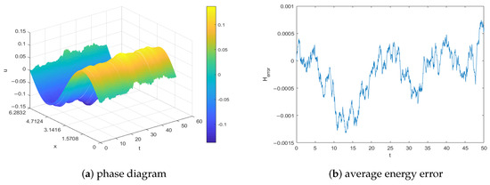
Figure 1. Phase diagram and conservative property of the LDG method for Example 1.

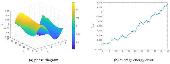
Figure 2. Phase diagram and conservative properties of the Galerkin spectral element method for Example 1.

Secondly, the spatial error of the LDG method is estimated as the mean-square sample error over 1000 different discretized sample paths, being displayed in a log–log plot in Figure 3 and in Table 1. For each numerical sample path, the LDG method is applied with four different spatial step sizes: $h=\pi /20$, $h=\pi /40$, $h=\pi /80$, and $h=\pi /160$. The reference solution is taken as the numerical solution with $N=1000$ and $h=\pi /320$. In this example, as we can see in Figure 3 and Table 1, the LDG method presents a spatial convergence rate of order 3.

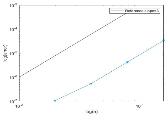
Figure 3. Spatial convergence order curve of the LDG method for Example 1.

Table 1. Spatial errors and convergence order of the LDG method for Example 1.

h	${\mathit{L}}^2$ Error	Order
$\pi /20$	$3.35\times {10}^{-5}$	–
$\pi /40$	$4.19\times {10}^{-6}$	3.00
$\pi /80$	$5.29\times {10}^{-7}$	2.98
$\pi /160$	$1.04\times {10}^{-7}$	2.35

6.2. Example 2

This example is to illustrate the influence of noise intensity on the LDG method. We respectively select the the coefficients in (1) with larger and smaller noise, under which conditions ${\alpha }^2-2a=0$ and ${\beta }^2+2c=0$ still hold. The other parameters are selected as in Example 1. Figure 4a,b displays the phase diagram and average sample energy error of the LDG method for (1) with larger noise intensity $\alpha =0.08$ and $\beta =0.08$, while Figure 4c,d shows the behaviors of the LDG method for (1) with smaller noise intensity $\alpha =0.01$ and $\beta =0.01$.

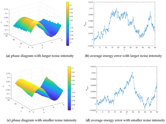
Figure 4. Phase diagrams and conservative properties of the LDG method for Example 2.

6.3. Example 3

Set the coefficients in (1) as $a=0.08$, $b=0.008$, $c=-0.08$, $\alpha =0.01$, and $\beta =0.01$. The other parameters are selected as in Example 1. In this case, ${\alpha }^2-2a<0$ and ${\beta }^2+2c<0$. We can see from the simulation of energy in Figure 5 that after a certain amount of time, the average energy tends to approach 0.

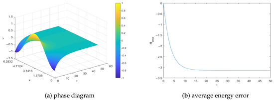
Figure 5. Phase diagram and conservative properties of the LDG method for Example 3.

7. Conclusions

In this paper, we propose a structure-preserving LDG method for parabolic stochastic partial differential equations. We show that under certain conditions, the numerical method is $L^2$ stable and can also maintain energy conservation. At the same time, we also prove that the method can achieve an accuracy of $n+1$ in space and verify the correctness of the theoretical results through several numerical examples.

References

- Liu, T. Porosity reconstruction based on Biot elastic model of porous media by homotopy perturbation method. Chaos Solitons Fractals 2022, 158, 112007. [Google Scholar] [CrossRef]
- Liu, T.; Li, T.; Ullah, M.Z. On five-point equidistant stencils based on Gaussian function with application in numerical multi-dimensional option pricing. Comput. Math. Appl. 2024, 176, 11. [Google Scholar] [CrossRef]
- Khattab, A.G.; Semary, M.S.; Hammad, D.A.; Fathy, A. Exploring stochastic heat equations: A numerical analysis with fast discrete Fourier transform techniques. Axioms 2024, 13, 886. [Google Scholar] [CrossRef]
- Fareed, A.F.; Semary, M.S. Stochastic improved Simpson for solving nonlinear fractional-order systems using product integration rules. Nonlinear Eng. 2025, 14, 20240070. [Google Scholar] [CrossRef]
- Fareed, A.F.; Semary, M.S.; Hassan, H.N. Two semi-analytical approaches to approximate the solution of stochastic ordinary differential equations with two enormous engineering applications. Alex. Eng. J. 2022, 61, 11935–11945. [Google Scholar] [CrossRef]
- Arif, M.S.; Abodayeh, K.; Nawaz, Y. A reliable computational scheme for stochastic reaction–diffusion nonlinear chemical model. Axioms 2023, 12, 460. [Google Scholar] [CrossRef]
- Arif, M.S.; Abodayeh, K.; Nawaz, Y. A computational scheme for stochastic non-Newtonian mixed convection nanofluid flow over oscillatory sheet. Energies 2023, 16, 2298. [Google Scholar] [CrossRef]
- Nawaz, Y.; Arif, M.S.; Nazeer, A.; Abbasi, J.N.; Abodayeh, K. A two-stage reliable computational scheme for stochastic unsteady mixed convection flow of Casson nanofluid. Int. J. Numer. Methods Fluids 2024, 96, 719–737. [Google Scholar] [CrossRef]
- Babaei, A.; Banihashemi, S.; Moghaddam, B.P.; Dabiri, A.; Galhano, A. Efficient solutions for stochastic fractional differential equations with a neutral delay using Jacobi poly-fractonomials. Mathematics 2024, 12, 3273. [Google Scholar] [CrossRef]
- Aryani, E.; Babaei, A.; Valinejad, A. A numerical technique for solving nonlinear fractional stochastic integro-differential equations with n-dimensional Wiener process. Comput. Methods Differ. Equ. 2022, 10, 61–76. [Google Scholar]
- Liu, T.; Ding, B.; Saray, B.N.; Juraev, D.A.; Elsayed, E.E. On the pseudospectral method for solving the fractional Klein–Gordon equation using Legendre cardinal functions. Fractal Fract. 2025, 9, 177. [Google Scholar] [CrossRef]
- Liu, T. Parameter estimation with the multigrid-homotopy method for a nonlinear diffusion equation. J. Comput. Appl. Math. 2022, 413, 114393. [Google Scholar] [CrossRef]
- Liu, Z.; Qiao, Z. Strong approximation of monotone stochastic partial differential equations driven by white noise. IMA J. Numer. Anal. 2020, 40, 1074–1093. [Google Scholar] [CrossRef]
- Mukam, J.D. Some Numerical Techniques for Approximating Semilinear Parabolic (Stochastic) Partial Differential Equations; Technische Universität Chemnitz: Chemnitz, Germany, 2021. [Google Scholar]
- Cui, J.; Hong, J. Strong and weak convergence rates of a spatial approximation for stochastic partial differential equation with one-sided Lipschitz coefficient. SIAM J. Numer. Anal. 2019, 57, 1815–1841. [Google Scholar] [CrossRef]
- Jin, B.; Yan, Y.; Zhou, Z. Numerical approximation of stochastic time-fractional diffusion. ESAIM Math. Model. Numer. Anal. 2019, 53, 1245–1268. [Google Scholar] [CrossRef]
- Peng, G.; Gao, Z.; Feng, X. A stabilized extremum-preserving scheme for nonlinear parabolic equation on polygonal meshes. Int. J. Numer. Methods Fluids 2019, 90, 340–356. [Google Scholar] [CrossRef]
- Yan, J.; Shu, C.W. Local discontinuous Galerkin methods for partial differential equations with higher order derivatives. J. Sci. Comput. 2002, 17, 27–47. [Google Scholar] [CrossRef]
- Chen, C.; Hong, J.; Ji, L. Mean-square convergence of a symplectic local discontinuous Galerkin method applied to stochastic linear Schrödinger equation. IMA J. Numer. Anal. 2017, 37, 1041–1065. [Google Scholar] [CrossRef]
- Li, Y. A high-order numerical method for BSPDEs with applications to mathematical finance. SIAM J. Financ. Math. 2022, 13, 147–178. [Google Scholar] [CrossRef]
- Li, Y. A high-order numerical scheme for stochastic optimal control problem. J. Comput. Appl. Math. 2023, 427, 115158. [Google Scholar] [CrossRef]
- Wang, H.; Tao, Q.; Shu, C.W.; Zhang, Q. Analysis of local discontinuous Galerkin methods with implicit-explicit time marching for linearized KdV equations. SIAM J. Numer. Anal. 2024, 62, 2222–2248. [Google Scholar] [CrossRef]
- Zhang, L.; Ji, L. Stochastic multi-symplectic Runge–Kutta methods for stochastic Hamiltonian PDEs. Appl. Numer. Math. 2019, 135, 396–406. [Google Scholar] [CrossRef]
- Zhou, Y.; Wang, Q.; Zhang, Z. Physical properties preserving numerical simulation of stochastic fractional nonlinear wave equation. Commun. Nonlinear Sci. Numer. Simul. 2021, 99, 105832. [Google Scholar] [CrossRef]
- Hou, B. Meshless structure-preserving GRBF collocation methods for stochastic Maxwell equations with multiplicative noise. Appl. Numer. Math. 2023, 192, 337–355. [Google Scholar] [CrossRef]
- Bai, G.; Hu, J.; Li, B. High-Order mass-and energy-conserving methods for the nonlinear Schrödinger equation. SIAM J. Sci. Comput. 2024, 46, A1026–A1046. [Google Scholar] [CrossRef]
- Mao, X. Stochastic Differential Equations and Their Applications; Harwood: Chichester, UK, 1997. [Google Scholar] [CrossRef]
- Kuo, H.H. Introduction to Stochastic Integration; Springer: New York, NY, USA, 2006. [Google Scholar] [CrossRef]
- He, S.W.; Wang, J.G.; Yan, J.A. Semimartingale Theory and Stochastic Calculus; Routledge: London, UK, 1992; p. 400. [Google Scholar]
Disclaimer/Publisher’s Note: The statements, opinions and data contained in all publications are solely those of the individual author(s) and contributor(s) and not of MDPI and/or the editor(s). MDPI and/or the editor(s) disclaim responsibility for any injury to people or property resulting from any ideas, methods, instructions or products referred to in the content. |
© 2025 by the authors. Licensee MDPI, Basel, Switzerland. This article is an open access article distributed under the terms and conditions of the Creative Commons Attribution (CC BY) license (https://creativecommons.org/licenses/by/4.0/).