Numerical Method for Band Gap Structure and Dirac Point of Photonic Crystals Based on Recurrent Neural Network

Abstract

In this paper, we propose a recurrent neural network numerical method with the finite element method for partial differential equations to study the band gap structure and Dirac points in two-dimensional photonic crystals. Electromagnetic wave propagation is governed by Maxwell’s equations. We transform the partial differential equations into large-scale generalized eigenvalue problems by spatially discretising them using the finite element method. Compared with traditional numerical computation methods, neural networks can perform high-speed parallel computation. Existing neural network-based eigenvalue solvers are typically restricted to computing extremal eigenvalues of real symmetric matrix pairs. To overcome this limitation, we develop a novel RNN-based numerical scheme tailored for solving the band structure problem in photonic crystals. We validate our method by computing the dispersion relations of photonic crystals with periodic dielectric columns, achieving excellent agreement with the plane-wave expansion method. In addition, we calculate the Dirac points at the center of the Brillouin zone, which is crucial for understanding the unique optical properties of photonic crystals. We determine the precise filling ratios at which these Dirac points appear, thus providing insight into the relationship between geometrical and material parameters and the appearance of Dirac points.

1. Introduction

Photonic crystals (PhCs) are novel optical materials composed of materials with varying dielectric constants arranged periodically in space. The most fundamental structural feature of PhCs is the photonic band gap (PBG), a unique structure that prohibits the propagation of photons in a certain frequency range. The PBG offers remarkable control over photon flow within the crystal, enabling a wide range of applications in optical devices and optical communication [1,2]. The laws of electromagnetic wave propagation in PhCs are usually described as a system of Maxwell’s equations. Calculating the energy band structure of PhCs is essentially solving a series of partial differential equations (PDEs) with multiple lowest least positive eigenvalues and corresponding eigenvectors. In the band structure of PhCs, the Dirac point is a special feature with a linear dispersion relation that plays a crucial role in condensed matter physics and classical wave systems. In 2011, C.T. Chan’s group discovered a Dirac-like cone at the center of the Brillouin zone in two-dimensional (2D) square lattice PhCs [3]. Leveraging the PBG principle allows control over photon propagation in PhCs, enabling the fabrication of diverse semiconductor photonic devices. Simultaneously, the photonic crystal energy band structure at the Dirac point exhibits linear dispersion, which gives rise to remarkable electronic-like properties. Notable phenomena such as boundary states [4], quantum Hall effects, pseudo-diffusive transmission, and zitterbewegung [5] have attracted significant attention from both academic research and industrial applications.

Numerous researchers have leveraged the powerful function approximation capabilities and flexibility of artificial neural networks (ANNs) to develop innovative methods for solving differential equations. Machine learning techniques such as Physics-Informed Neural Networks (PINNs) [6], Deep Galerkin Methods (DGMs) [7], and the Deep Ritz Method (DRM) [8] have emerged as prominent approaches for solving PDEs. Recent advancements have expanded these frameworks further, with novel neural network architectures [9,10,11,12,13,14] being proposed to address PDE challenges. However, these neural network methods primarily handle standard boundary conditions (e.g., Dirichlet and Neumann types) and non-coupled solution domains. Common numerical methods for simulating 2D PhC structures include the plane-wave expansion (PWE) method [15], the finite-difference time-domain (FDTD) method [16], the finite element method (FEM) [17], etc. The eigenvalue equations under investigation involve periodic boundary conditions within solution domains comprising dielectric materials of varying permittivity. Therefore, we propose to use the FEM to deal with the boundary conditions and the coupling of the region. Through integration with electromagnetic variational principles, we derive the finite element model for 2D PhCs directly from Maxwell’s equations. This FEM discretization yields large-scale generalized eigenvalue problems of the form $\mathit{A}\mathit{u}=\lambda \mathit{B}\mathit{u}$, where $\mathit{A}\in C^{n\times n}$ is a Hermitian matrix and $\mathit{B}\in R^{n\times n}$ is a real symmetric positive definite matrix.

Numerical methods for solving large-scale generalized eigenvalue problem, such as the subspace iteration method, Davidson’s method, and Lanczos’s method [18] have been extensively studied. Traditional algorithms are computationally expensive for such problems, while neural networks offer significant performance improvements through parallelization [19,20]. A Recurrent Neural Network (RNN) is an exemplary model for dynamic computation in neuroscience and machine learning, which has more computational power than feedforward neural networks and has a much better theoretical convergence rate compared to other previous correlated neural network methods [21,22,23]. This network has good convergence and evolves as a decreasing capacity function for a given initial state, eventually reaching a stable state. Not only does it function as an associative memory, it also shows remarkable potential in solving optimization problems. Since its energy function tends to be minimized, in principle, any optimization problem whose objective function can be expressed in the form of an energy function can be solved by using an RNN. Stability in this network is closely related to its capacity for associative memory. Researchers have proposed a large number of easy-to-simulate circuit implementations of RNN models for solving optimization problems as well as their highly parallel processing capabilities, including RNN models for solving matrix eigenvalue problems [24,25,26,27,28]. Mathematically, this neural network approach transforms the eigenvalue problem into a dynamical system of ordinary differential equations (ODEs), often termed neurodynamic optimization.

In this paper, we propose a new RNN model to compute the maximum eigenvalue of the generalized eigenvalue problem, where $\mathit{A}\in C^{n\times n}$ is a Hermitian matrix and $\mathit{B}\in R^{n\times n}$ is a real symmetric positive definite matrix. To compute all eigenvalues of the generalized eigenvalue problem in 2D PhCs, we develop an innovative algorithm based on our RNN model. Our motivation stems from the need for a more efficient and scalable solution to this complex problem, which is crucial for advancing the understanding and design of photonic structures. In Section 3, we present comprehensive numerical simulation results that validate the effectiveness of our proposed algorithm, including band structure calculations and visualizations for 2D square lattice PhCs with periodically arranged circular dielectric columns. Our simulations demonstrate remarkable agreement with results obtained from the traditional PWE method, confirming the reliability and accuracy of our RNN-based approach. Furthermore, our algorithm analyzes the band structure of 2D square lattice PhCs with different geometrical and material properties. By modulating the radius of the medium column and the functional form of the dielectric constant, we observe significant alterations in the number, width, and position of band gaps. Notably, the Dirac point (or semi-Dirac point) may emerge or vanish depending on these parameters, highlighting the intricate relationships within the photonic structures. To deepen our understanding of these phenomena, we calculate the Dirac points at the center of the Brillouin zone in 2D square lattice PhCs with periodically arranged circular and rectangular dielectric columns.

2. Method

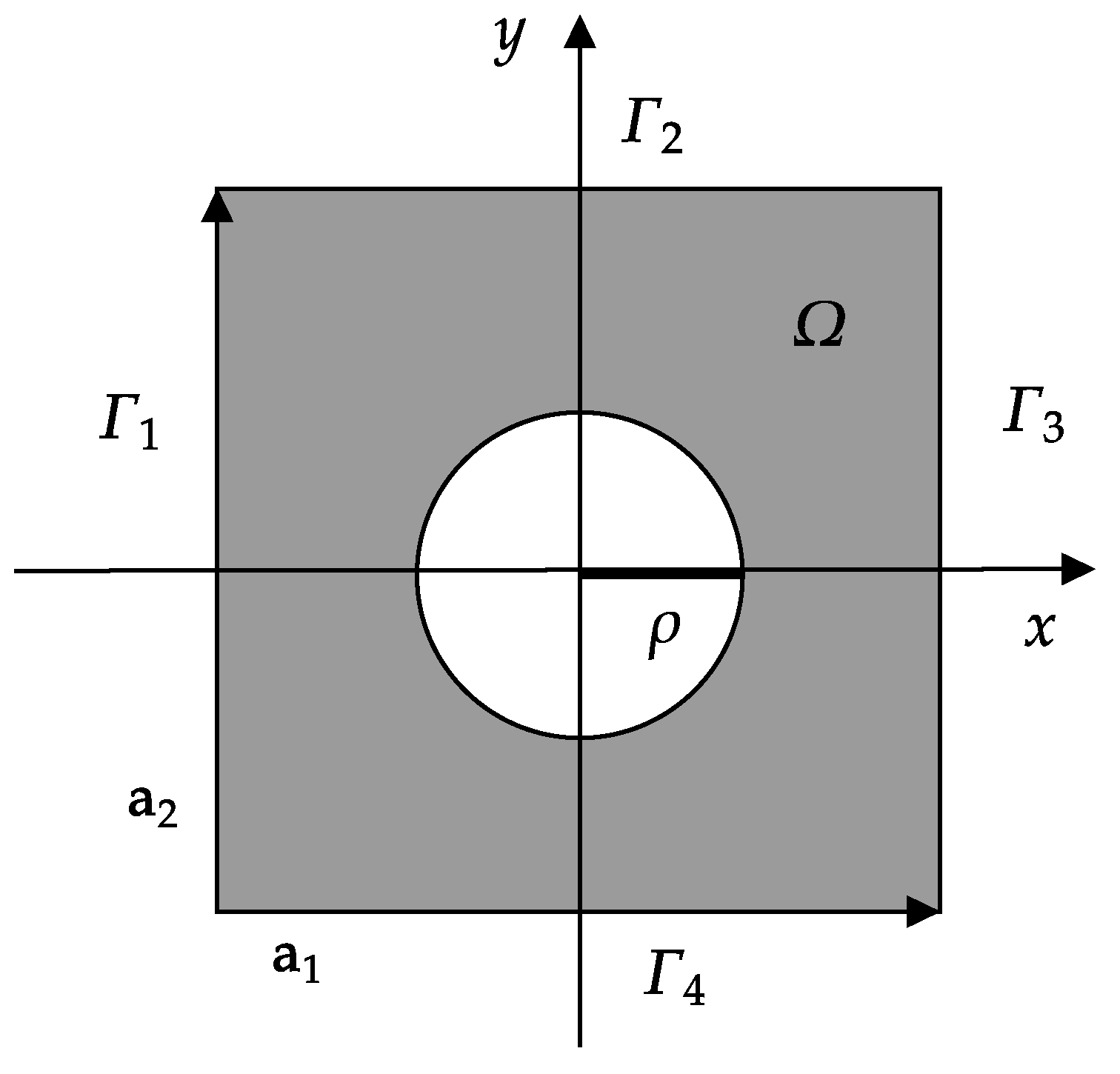
2.1. Model for Band Gap Calculation

We consider the computational model of the band structure in 2D square lattice PhCs, with its unit cell as shown in Figure 1. The lattice basis vectors are ${\mathit{a}}_{\mathbf{1}}=L{\mathit{e}}_{\mathit{x}}$ and ${\mathit{a}}_{\mathbf{2}}=L{\mathit{e}}_{\mathit{y}}$, where L is the lattice constant and ${\mathit{e}}_{\mathit{x}}$, ${\mathit{e}}_{\mathit{y}}$ are unit vectors. The domain $\mathsf{\Omega }$ is the square region bounded by ${\mathsf{\Gamma }}_1$, ${\mathsf{\Gamma }}_2$, ${\mathsf{\Gamma }}_3$, and ${\mathsf{\Gamma }}_4$, where ${\mathsf{\Gamma }}_1$ is parallel to ${\mathsf{\Gamma }}_3$ and ${\mathsf{\Gamma }}_2$ is parallel to ${\mathsf{\Gamma }}_4$. The 2D PhCs are artificial structures formed by periodically arranged dielectric columns, with the dielectric constant of the dielectric column being ${\epsilon }_2$ and that of the background medium being ${\epsilon }_1$. We assume that the radius of each dielectric column is $\rho$ and the relative dielectric function is

$$\epsilon \left(\mathit{r}\right)=\left\{\begin{array}{c}{\epsilon }_2,\mathrm{if}|\mathit{r}-l_1{\mathit{a}}_{\mathbf{1}}-l_2{\mathit{a}}_{\mathbf{2}}|<\rho ;\hfill \\ {\epsilon }_1,\mathrm{otherwise},\hfill \end{array}\right.$$

(1)

where $\mathit{r}=(x,y)$ represents the coordinates and $l_1$ and $l_2$ are arbitrary integers.

Photonic band structures are governed by the eigenvalue problems derived from the Maxwell’s equations:

$$\left\{\begin{array}{c}\nabla \times \mathit{E}+i\omega \mu \mathit{H}=0\hfill \\ \nabla \times \mathit{H}-i\omega \epsilon \mathit{E}=0\hfill \end{array}.\right.$$

(2)

We assume that the magnetic permeability $\mu$ is constant. Since the electromagnetic waves can be decomposed into harmonic waves as $\mathit{E}\left(\mathit{r},t\right)=\mathit{E}\left(\mathit{r}\right)e^{-i\omega t}$, $\mathit{H}\left(\mathit{r},t\right)=\mathit{H}\left(\mathit{r}\right)e^{-i\omega t}$, where $\mathit{E}\left(\mathit{r},t\right)$ and $\mathit{H}\left(\mathit{r},t\right)$ are the electric and magnetic field strength and $\omega$ is the angular frequency. We then substitute these into Equation (2) to obtain the Helmholtz equations, which are independent of the time variable [8]:

$$\left\{\begin{array}{c}{\displaystyle \frac{1}{\epsilon \left(\mathit{r}\right)}}\nabla \times \nabla \times \mathit{E}\left(\mathit{r}\right)={\left({\displaystyle \frac{\omega }{c}}\right)}^2\mathit{E}\left(\mathit{r}\right)\hfill \\ \nabla \times \left({\displaystyle \frac{1}{\epsilon \left(\mathit{r}\right)}}·\nabla \times \mathit{H}\left(\mathit{r}\right)\right)={\left({\displaystyle \frac{\omega }{c}}\right)}^2\mathit{H}\left(\mathit{r}\right)\hfill \end{array}\mathrm{in}\mathsf{\Omega }\right.$$

(3)

where c is the speed of light in air. When we analyze the PBG problem in 2D PhCs, the problem can be simplified into two polarization cases: TM (transverse magnetic) and TE (transverse electric), where $\mathit{E}\left(\mathit{r}\right)=(0,0,u(x,y))$ for TM polarization and $\mathit{H}\left(\mathit{r}\right)=(0,0,u(x,y))$ for TE polarization. Introducing the wave vector $\mathit{k}=(\alpha ,\beta )$ into the first Brillouin zone $B_f$ of the square lattice as shown in Figure 2, the irreducible Brillouin region $B_f$ is the triangular region bounded by $\mathsf{\Gamma }=2\pi /L(0,0)$, $X=2\pi /L(1/2,0)$, and $M=2\pi /L(1/2,1/2)$.

According to Bloch’s principle, the wave function $u\left(\mathit{r}\right)$ can be described as $u\left(\mathit{r}\right)=e^{i\mathit{k}·\mathit{r}}{u}_R\left(\mathit{r}\right)$, where $u_R\left(\mathit{r}\right)$ is the Floquet transform of $u\left(\mathit{r}\right)$, ensuring periodicity in the x and y directions. For notational simplicity, we replace $u_R$ with u. Substituting the wave function into Equation (3) yields PDEs with periodic boundary conditions:

$$\left\{\begin{array}{c}(\nabla +i\mathit{k})·\left[\varrho (\nabla +i\mathit{k})u\right]+{\omega }^2\kappa u=0,\mathrm{in}\mathsf{\Omega }\hfill \\ {u|}_{{\mathsf{\Gamma }}_1}{=u|}_{{\mathsf{\Gamma }}_3},u{{|}_{{\mathsf{\Gamma }}_2}=u|}_{{\mathsf{\Gamma }}_4},\mathrm{on}\partial \mathsf{\Omega }\hfill \end{array}\right.$$

(4)

where the material coefficients are $\varrho =\left\{\begin{array}{cc}1,& TM\\ {\displaystyle \frac{1}{\epsilon \left(\mathit{r}\right)}},& TE\end{array}\right.$ and $\kappa =\left\{\begin{array}{cc}{\displaystyle \frac{\epsilon \left(\mathit{r}\right)}{c^2}},& TM\\ {\displaystyle \frac{1}{c^2}},& TE\end{array}\right.$.

2.2. Finite Element Schemes

Define the complete Sobolev space

$$\mathbb{X}=\left\{v|v\in H^1\left(\mathsf{\Omega }\right),\mathrm{and}{v|}_{{\mathsf{\Gamma }}_1}={v|}_{{\mathsf{\Gamma }}_3},{v|}_{{\mathsf{\Gamma }}_2}={v|}_{{\mathsf{\Gamma }}_4}\right\}$$

where $H^1\left(\mathsf{\Omega }\right)$ is Hilbert space and $\mathsf{\Omega }$ denotes the computational region. The norm of $\mathsf{\Omega }$ space is ${\left|\right|v\left|\right|}_1={\left|\right|\nabla v\left|\right|}_{L^2\left(\mathsf{\Omega }\right)}+{\left|\right|v\left|\right|}_{L^2\left(\mathsf{\Omega }\right)}$, $\forall v\in \mathbb{X}$, where $\left|\right|·{\left|\right|}_{L^2\left(\mathsf{\Omega }\right)}$ is the norm of $L^2\left(\mathsf{\Omega }\right)$ space. Following Galerkin’s variational principle and applying continuous boundary conditions, we have

$$〈\varrho (\nabla +i\mathit{k})u,(\nabla +i\mathit{k})v〉-{\omega }^2〈\kappa u,v〉=0,\forall v\in \mathbb{X}$$

where $〈·,·〉$ is the standard inner product of $L^2\left(\mathsf{\Omega }\right)$ space. Then Equation (4) can be written as the following variational problem: given vector $\mathit{k}\in B_f$, find $u\in \mathbb{X}$ and $\omega$ such that

$$a(u,v)={\omega }^{2}b(u,v),v\in \mathbb{X}$$

(5)

where $a(u,v)=〈\varrho (\nabla +i\mathit{k})u,(\nabla +i\mathit{k})v〉$ and $b(u,v)=〈\kappa u,v〉$ are the bilinear forms.

The linear finite element discretization method is used to solve the weak form above. First, we discretize the solution region $\mathsf{\Omega }$ by using triangular mesh, designated as M. The discrete solution space corresponding to solution space $\mathbb{X}$ is ${\mathbb{X}}_h$ as

$${\mathbb{X}}_h=\left\{v_h{|v_h\in \mathbb{X},v_h|}_K=a_K+b_{K}x+c_{K}y,\left\{a_K,b_K,c_K\right\}\in \mathrm{R},K\in M\right\},$$

which satisfies the boundary conditions, and K is the triangular element code. We define the norm of a function in the space ${\mathbb{X}}_h$ as the norm in the space $\mathbb{X}$. There are test functions $v_h\in {\mathbb{X}}_h$ defined on the triangular elements, and the finite element discretization problem corresponding to the variational problem can be described as follows: given vector $\mathit{k}\in B_f$, find $u_h\in {\mathbb{X}}_h$ and ${\omega }_h$ such that

$$a(u_h,v_h)={\omega }_h^{2}b(u_h,v_h),v_h\in {\mathbb{X}}_h.$$

According to the discrete linear equations system, we obtain the cell stiffness matrices and generate the total stiffness matrices $\mathit{A}$ and $\mathit{B}$ based on the local numbering and overall numbering relationships of the linear triangular elements.

After imposing periodic boundary conditions, we reduce Equation (4) to the form of the large-scale generalized eigenvalue problem

$$\mathit{A}\mathit{u}=\lambda \mathit{B}\mathit{u}$$

(6)

where $\mathit{A}\in C^{n\times n}$ is a Hermitian matrix and $\mathit{B}\in R^{n\times n}$ is a real symmetric positive definite matrix. For the wave vector $\mathit{k}$ traversing the boundary of the first Brillouin zone, we can then obtain the PBG structure.

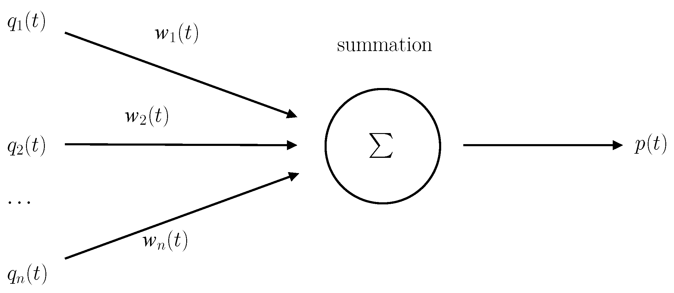
2.3. RNN Model and Algorithm

For the large-scale generalized eigenvalue problem, we propose a new neural network model based on the RNN architecture and an associated algorithm to compute all generalized eigenvalues. We consider the following single-layer linear neural network model, as shown in Figure 3. The neural network is structured with three layers: the input layer, the hidden layer, and the output layer. There are different numbers of neurons on each layer. The neurons in different layers are interconnected with varying degrees of linkage, where the strength of these connections is represented by the weight vector, denoted as $\mathit{w}\left(t\right)=(w_1\left(t\right),w_2\left(t\right),\cdots ,w_n\left(t\right))$. The operation of the linear neural network can be viewed as computing a function:

$$p\left(t\right)=\sum _{i=1}^n{w}_i\left(t\right)q_i\left(t\right)={\mathit{w}}^T\left(t\right)\mathit{q}\left(t\right),$$

(7)

where $\mathit{q}\left(t\right)=(q_1\left(t\right),q_2\left(t\right),\cdots ,q_n\left(t\right))$ represents the input vector at time step t and $p\left(t\right)$ represents the output of the neural network, the activation function is linear. There is only one neuron in the output layer and t is the number of iterations.

Building on the neural network model described above, several studies have employed RNN models integrated with neurodynamic optimization approaches to compute the maximum or minimum generalized eigenvalues of matrix pairs. These methods are not only efficient but also highly parallelizable, making them suitable for large-scale computational problems. In 2006, Liu [27] proposed an algorithm based on an RNN model to compute the largest eigenvalue and its corresponding eigenvector of the generalized eigenvalue problem:

$$\tilde{\mathit{A}}\mathit{x}=\lambda \tilde{\mathit{B}}\mathit{x}$$

(8)

where $\tilde{\mathit{A}}\in R^{n\times n}$ is a symmetric matrix and $\tilde{\mathit{B}}\in R^{n\times n}$ is a symmetric positive definite matrix. To iteratively update the weight vector, they introduced the following discrete-time update rule:

$$\mathit{x}(t+1)=\mathit{x}\left(t\right)+\eta ({\mathit{x}}^T\left(t\right)\tilde{\mathit{B}}\mathit{x}\left(t\right){\tilde{\mathit{B}}}^{-1}\tilde{\mathit{A}}\mathit{x}\left(t\right)-{\mathit{x}}^T\left(t\right)\tilde{\mathit{A}}\mathit{x}\left(t\right)\mathit{x}\left(t\right)),t\ge 0$$

(9)

where $0<\eta <1$ is the learning rate of the neural network and t is the number of iterations. Furthermore, Liu formulated a continuous-time RNN model to describe the dynamic evolution of $\mathit{x}\left(t\right)$ and rigorously demonstrated its convergence:

$${\displaystyle \frac{d\mathit{x}\left(t\right)}{dt}}={\mathit{x}}^T\left(t\right)\tilde{\mathit{B}}\mathit{x}\left(t\right){\tilde{\mathit{B}}}^{-1}\tilde{\mathit{A}}\mathit{x}\left(t\right)-{\mathit{x}}^T\left(t\right)\tilde{\mathit{A}}\mathit{x}\left(t\right)\mathit{x}\left(t\right),t\ge 0.$$

(10)

Considering the generalized eigenvalue problem (6), the objective of the neural network algorithm is to establish a suitable learning rule for updating the network’s weight vector. This learning rule ensures that the weight vector converges to the eigenvector corresponding to the largest eigenvalue of the matrix pair $(\mathit{A},\mathit{B})$. To achieve this, we similarly propose the following neural network weight vector updating algorithm and illustrate its effectiveness through arithmetic examples:

$$\mathit{u}(t+1)=\mathit{u}\left(t\right)+\eta ({\mathit{u}}^T\left(t\right)\mathit{B}\mathit{u}\left(t\right){\mathit{B}}^{-1}\mathit{A}\mathit{u}\left(t\right)-{\mathit{u}}^T\left(t\right)\mathit{A}\mathit{u}\left(t\right)\mathit{u}\left(t\right)),t\ge 0$$

(11)

where $0<\eta <1$ is the learning rate and $\mathit{u}\left(t\right)$ is the state of the neural network. This equation essentially defines a Hopfield neural network-based update rule for the weight vector. The network’s output typically converges to the eigenvector associated with the largest generalized eigenvalue, effectively solving the optimization problem in an iterative manner.

According to stochastic approximation theory, the convergence of the stochastic recursive Equation (11) is equivalent to the stability of the corresponding continuous ODE system, also referred to as the RNN model, which is described as follows:

$${\displaystyle \frac{d\mathit{u}\left(t\right)}{dt}}={\mathit{u}}^T\left(t\right)\mathit{B}\mathit{u}\left(t\right){\mathit{B}}^{-1}\mathit{A}\mathit{u}\left(t\right)-{\mathit{u}}^T\left(t\right)\mathit{A}\mathit{u}\left(t\right)\mathit{u}\left(t\right),t\ge 0.$$

(12)

The eigenvector associated with the largest generalized eigenvalue serves as the stable equilibrium of the neural network. This implies that, for any initial vector, the solution of (11) will converge to the eigenvector $\mathit{u}$ corresponding to the maximum generalized eigenvalue of the matrix pair $(\mathit{A},\mathit{B})$. To compute the eigenvector associated with the maximum eigenvalue, we typically solve this ODE system using the Runge–Kutta method, setting the relative tolerance ${ϵ}_{rel}=10$$\times {10}^{-3}$ and the absolute tolerance ${ϵ}_{abs}=10$$\times {10}^{-6}$. This approach optimizes computational efficiency by using the difference between the 4th- and 5th-order solutions at each step as an estimate of the local truncation error and adaptively adjusting the step size based on a weighted norm of this error. The corresponding maximum generalized eigenvalue can then be obtained using the Rayleigh quotient $\beta \left(t\right)={\displaystyle \frac{{\mathit{u}}^T\left(t\right)\mathit{A}\mathit{u}\left(t\right)}{{\mathit{u}}^T\left(t\right)\mathit{B}\mathit{u}\left(t\right)}}$.

After computing the maximum eigenvalue, we now outline the algorithm for determining the remaining eigenvalues of the generalized eigenvalue problem (see Algorithm 1). Utilizing the computed maximum eigenvalue, we construct a systematic approach to sequentially obtain all eigenvalues in descending order. Specifically, we propose the following algorithm, based on the neural network model (12), for computing the eigenvalues ${\lambda }_1\ge {\lambda }_2\ge \cdots \ge {\lambda }_n$ in descending order. In this algorithm, the largest eigenvalue ${\lambda }_1$ is first calculated based on the given RNN model (12). Subsequently, the matrix $\mathit{A}$ is iteratively updated through the deflation operator $\mathit{A}\leftarrow \mathit{A}(I-{\displaystyle \sum _{k=1}^{i-1}}{\mathit{e}}_k{\mathit{e}}_k^H)$, where $e_i$ for $i=1,\cdots ,n$ denotes the orthonormal eigenvector obtained by applying schmidt orthogonalization to $u_i$. Through this process, it can be rigorously shown that ${\lambda }_k=0$ for $k=1,\cdots ,i$ and ${\lambda }_{i+1}$ is the largest eigenvalue. To ensure spectral non-negativity, a stabilization term $\alpha \mathit{B}$ is incorporated into the matrix $\mathit{A}$. This systematic approach enables sequential determination of all eigenvalues for the generalized eigenvalue problem (6) in descending order.

Algorithm 1 RNN algorithm for generalized eigenvalue problem

Input: Hermitian matrix $\mathit{A}$, real symmetric matrix $\mathit{B}$, matrix dimension n, solution interval $[0,t]$, arbitrary constant $\alpha >0$ Output: eigenvalues ${\lambda }_1,\cdots ,{\lambda }_n$       1: for i = 1 to n do       2:    let ${\mathit{A}}_i={\mathit{A}}_{i-1}(I-{\displaystyle \sum _{k=1}^{i-1}}{\mathit{e}}_k{\mathit{e}}_k^H)+\alpha \mathit{B}$ where ${\mathit{A}}_0=\mathit{A}$ and set initial random vector ${\mathit{u}}_i\left(0\right)$       3:    compute ${\displaystyle \frac{d{\mathit{u}}_i\left(t\right)}{dt}}={\mathit{u}}_i^T\left(t\right)\mathit{B}{\mathit{u}}_i\left(t\right){\mathit{B}}^{-1}{\mathit{A}}_i{\mathit{u}}_i\left(t\right)-{\mathit{u}}_i^T\left(t\right){\mathit{A}}_i{\mathit{u}}_i\left(t\right){\mathit{u}}_i\left(t\right)$       4:    get ${\lambda }_i$ by ${\displaystyle \frac{{\mathit{u}}_i^T\left(t\right){\mathit{A}}_i{\mathit{u}}_i\left(t\right)}{{\mathit{u}}_i^T\left(t\right)\mathit{B}{\mathit{u}}_i\left(t\right)}}$ and schmidt orthogonalization of ${\mathit{u}}_1,\cdots ,{\mathit{u}}_i$ yields unit eigenvectors ${\mathit{e}}_1,\cdots ,{\mathit{e}}_i$       5: end for

This algorithm leverages the neural network’s ability to iteratively converge to the desired eigenvectors and eigenvalues, providing a robust and efficient method for solving the generalized eigenvalue problem. In summary, the overall process regarding solving Equation (4) for photonic crystal structures is as follows (Figure 4).

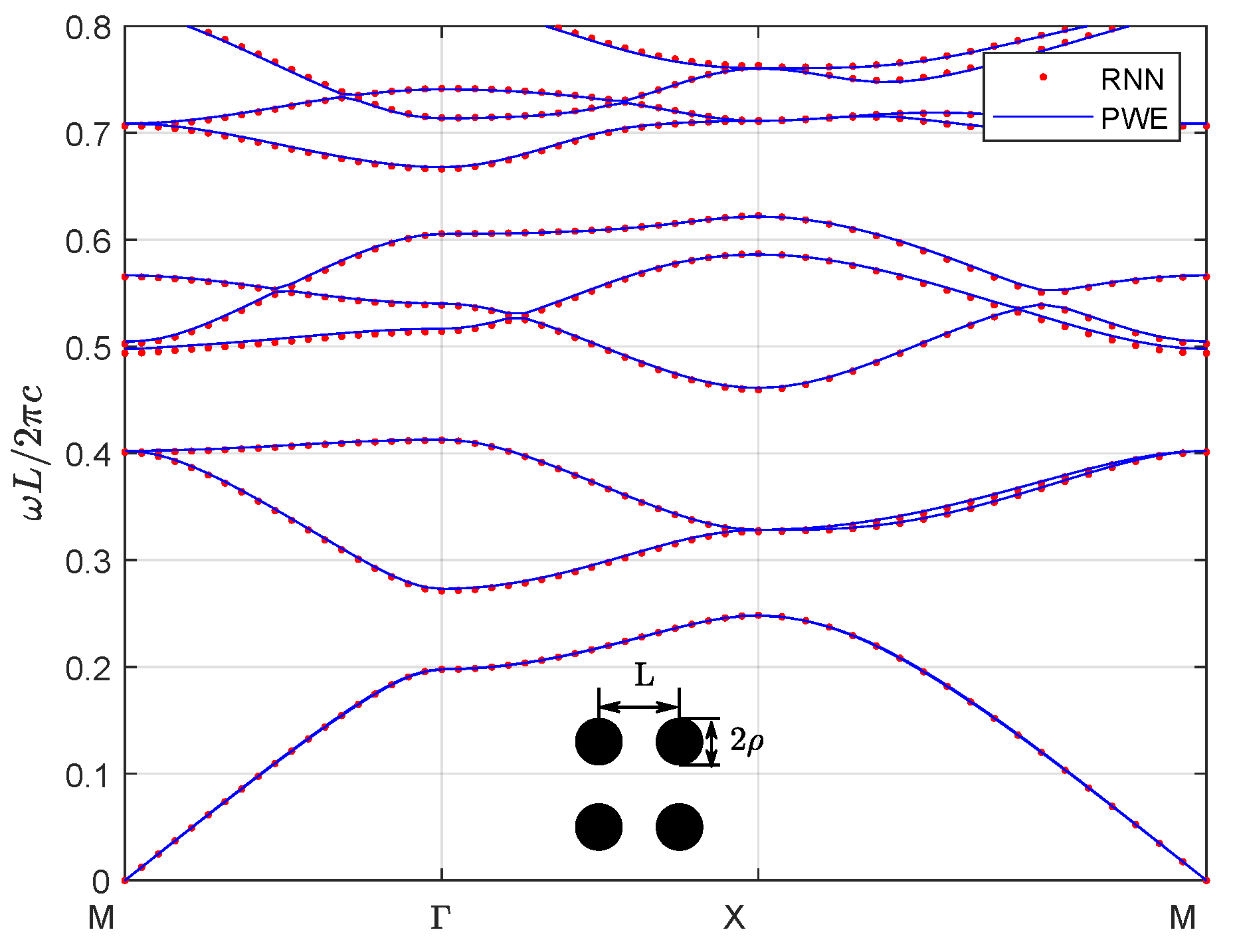
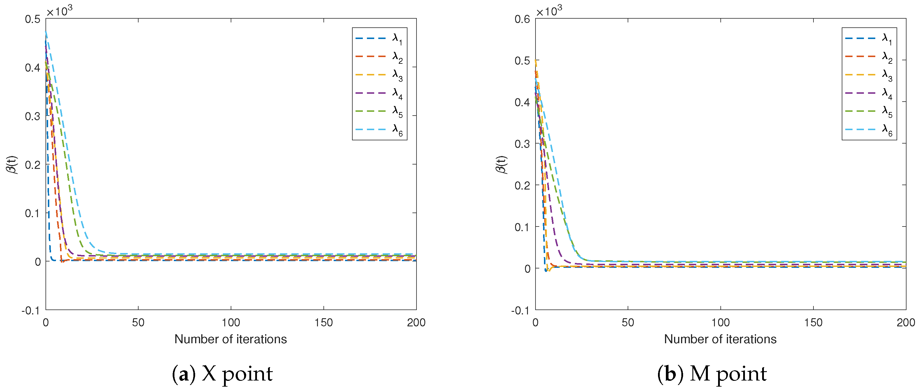
3. Numerical Calculation

In order to validate our approach, we present several numerical examples of 2D PhCs composed of a background medium and dielectric columns in this section. We use the finite element meshing method for Equation (4), which yields generalized eigenvalue problem matrices of a scale in the thousands. For the first numerical example, we consider 2D square lattice PhCs with periodically arranged circular dielectric columns. In the x-y plane, the circular dielectric columns are evenly arranged in the square lattice against an air background and extend infinitely along the z-axis. The background medium is air, with a dielectric constant of ${\epsilon }_1=1$, and the dielectric column material is Aluminum Nitride (AlN), with a dielectric constant of ${\epsilon }_2=8.9$. The chosen structural parameters are as follows: the lattice constant is $L=1$ and the radius of dielectric column is $\rho =0.375L$. We use our proposed algorithm to calculate the band structure for TM polarization and compare these results with those obtained using the PWE method, as depicted in Figure 5. We also calculate the relative errors $\xi$ between the results from our RNN model and the PWE method for the first ten bands that are displayed in

Table 1. Relative error: the relative errors $\xi$ for the RNN method and PWE method for first ten bands.

Band	$\mathit{\xi }$	Band	$\mathit{\xi }$
1	1.28 $\times {10}^{-3}$	6	2.10 $\times {10}^{-3}$
2	1.83 $\times {10}^{-3}$	7	2.47 $\times {10}^{-3}$
3	5.10 $\times {10}^{-4}$	8	4.87 $\times {10}^{-3}$
4	1.58 $\times {10}^{-3}$	9	7.26 $\times {10}^{-3}$
5	2.93 $\times {10}^{-4}$	10	7.92 $\times {10}^{-3}$

. For TM polarization, the normalized frequency ranges of forbidden bands are as follows: 0.2483∼0.2713, 0.4122∼0.4594, and 0.6226∼0.6663.

Also, to further validate the effectiveness and convergence performance of the proposed algorithm, we analyze the transient behavior of the Rayleigh quotient $\beta \left(t\right)={\displaystyle \frac{{\mathit{u}}^T\left(t\right)\mathit{A}\mathit{u}\left(t\right)}{{\mathit{u}}^T\left(t\right)\mathit{B}\mathit{u}\left(t\right)}}$ for the first six eigenvalues at the M and X symmetry points by using the RNN method. As shown in Figure 6, the RNN model demonstrates robust and rapid convergence to stable solutions.

We next investigate the PBG properties in the square lattice for TM polarization by varying the radius $\rho$ of the dielectric column while fixing other parameters. As shown in Figure 7, as the dielectric filling ratio $\rho /L$ gradually increases to approximately 0.1, the PBG emerges and its width gradually widens. However, as the dielectric filling ratio continues to increase and reaches its maximum value, the bandwidth begins to gradually decrease and eventually narrows and disappears at a specific point. During this process, the position of the PBG shifts to lower frequencies as the dielectric filling ratio increases. Specifically, the first PBG appears at $\rho /L=0.096$ and reaches its maximum bandwidth at $\rho /L=0.190$, and then disappears at $\rho /L=0.420$. Similarly, the second PBG emerges at $\rho /L=0.230$ and reaches its maximum bandwidth at $\rho /L=0.324$.

Next, for the second numerical example, we consider a new kind of wide-bandgap semiconductor material BiNbO4, which exhibits exceptional properties and significant potential for various applications. BiNbO4 ceramics are low-temperature sintered materials exhibiting excellent microwave dielectric properties, including a high dielectric constant and low loss. These characteristics make them promising for broad applications in microwave communication, electronic components, and related fields [29]. BiNbO4 ceramics sintered at 1000 °C are relatively dense, and their dielectric properties vary little with frequency and temperature. The dielectric constants and dielectric losses of BiNbO4 ceramics sintered at 1 kHz and 1000 °C are 56.6 and 0.001, respectively [30]. We choose the same crystal structure as the first example above, the lattice constant is $L=1$ and the radius of the dielectric column is $\rho =0.378L$, and then calculate the band structure of the materials of the dielectric column for TM polarization, which is shown in Figure 8.

Further analysis reveals the following optimal conditions for maximizing the PBGs: the first gap reaches a maximum of 0.225 when the radius of the dielectric column is $\rho =0.122L$ in Figure 9. The second gap reaches a maximum of 0.1128 when the radius of the dielectric column is $\rho =0.230L$ in Figure 10. The third gap reaches a maximum of 0.1144 when the radius of the dielectric column is $\rho =0.234L$ in Figure 11.

Finally, leveraging the parallel and rapid computational capabilities of neural networks, we investigate the Dirac points in 2D square lattice PhCs with periodically arranged circular dielectric columns using the control variates method. In this study, the dielectric constant of the background medium is ${\epsilon }_1=1$ and that of the dielectric column is ${\epsilon }_2=12.5$. By continuously adjusting the filling ratios for calculation, we can obtain the same conclusion as the finding of C.T. Chan’s group [3]. For TM polarization, the band structure of the photonic lattice is shown in Figure 12. The chosen structural parameters are as follows: the lattice constant is $L=1$ and the radius of the dielectric column is $\rho =0.20L$. There is a triply degenerate point A at the $\mathsf{\Gamma }$ point, which is formed by accidental degeneracy. To further explore the behavior of the degenerate states, we keep the dielectric constant ${\epsilon }_2$ of the dielectric column unchanged and change the radius $\rho$. This adjustment causes the triply degenerate state to split into a two-fold degenerate state and a non-degenerate state. The frequency of the two-fold degenerate state is higher than that of the non-degenerate state at the $\mathsf{\Gamma }$ point when $\rho =0.19L$, as shown in Figure 13, and the frequency of the two-fold degenerate state is lower than that of the non-degenerate state at the $\mathsf{\Gamma }$ point when $\rho =0.21L$, as shown in Figure 14.

In the case where the background medium of the 2D square lattice PhCs with periodic circular dielectric columns fixed as air, the realization of the Dirac point is governed by two key variables: the filling ratio and the dielectric constant of dielectric column. To systematically explore how these variables influence Dirac point formation, we performed parameter studies by varying each quantity independently while holding others constant. The curve depicted in Figure 15 illustrates the relationship between the filling ratio and the dielectric constant required for the emergence of the Dirac point at the $\mathsf{\Gamma }$ point. Our analysis reveals a clear inverse correlation between these two parameters: as the dielectric constant of the dielectric column increases, the filling ratio necessary to achieve the Dirac point decreases. This trend highlights the delicate balance between the material properties and geometric configuration in the formation of Dirac points within photonic crystal structures. This inverse relationship can be attributed to the interplay between the electromagnetic field distribution and the periodic potential imposed by the photonic crystal lattice. Higher dielectric constants enhance the contrast in the refractive index, thereby strengthening the photonic band gap effects. Consequently, the formation of Dirac points requires a lower filling ratio.

Similarly, we examine a configuration of rectangular dielectric columns arranged in a square lattice against an air background, extending infinitely along the z-axis. Here, the dielectric constant of the background medium is ${\epsilon }_1=1$ and that of the dielectric column is ${\epsilon }_2=11.5$. The chosen structural parameters are as follows: the lattice constant is $L=1$ and the length of dielectric column is $\rho =0.185L$. There is also a triply degenerate point A at the $\mathsf{\Gamma }$ point for TM polarization, which is shown in Figure 16. When we change $\rho =0.185L$ to $0.175L$ and $0.195L$, the triply degenerate state splits into a two-fold degenerate state and a non-degenerate state. Specifically, the frequency of the two-fold degenerate state is higher than that of the non-degenerate state at the $\mathsf{\Gamma }$ point when $\rho =0.175L$, as shown in Figure 17, and the frequency of the two-fold degenerate state is lower than that of the non-degenerate state at the $\mathsf{\Gamma }$ point when $\rho =0.195L$, as shown in Figure 18. Keeping the background medium as air, we also investigate the influence of the filling ratio and the dielectric constant of the rectangular dielectric column at the Dirac points. The results of this analysis are presented in Figure 19, which illustrates the relationship between these parameters and the emergence of Dirac points.

4. Conclusions

In this paper, we propose a numerical method based on an RNN for solving the generalized eigenvalue problems arising from finite element discretization of Maxwell’s equations. To validate the accuracy and reliability of our method, we compare the results with those obtained by the PWE method. The numerical simulations demonstrate excellent agreement between the two approaches, confirming the effectiveness of our RNN-based algorithm. Furthermore, we investigate the conditions for the emergence of Dirac points at the $\mathsf{\Gamma }$ point in 2D square lattice PhCs, focusing on the influence of dielectric constants and filling ratios. This analysis is extended to PhCs with both circular and rectangular dielectric columns arranged periodically. These findings provide valuable insights into the design and optimization of photonic crystals for applications requiring precise control over Dirac point formation, such as in topological photonic and advanced optical communication systems.

References

1. Zong, Y.X.; Xia, J.B. Photonic band structure of two-dimensional metal/dielectric photonic crystals. J. Phys. D Appl. Phys. 2015, 48, 355103. [Google Scholar] [CrossRef]
2. Lu, S.; Li, W.; Guo, H.; Lu, M. Analysis of birefringent and dispersive properties of photonic crystal fibers. Appl. Opt. 2011, 50, 5798–5802. [Google Scholar] [CrossRef]
3. Huang, X.; Lai, Y.; Hang, Z.H.; Zheng, H.; Chan, C.T. Dirac cones induced by accidental degeneracy in photonic crystals and zero-refractive-index materials. Nat. Mater. 2011, 10, 582–586. [Google Scholar] [CrossRef]
4. Zhong, W.; Zhang, X. Acoustic analog of monolayer graphene and edge states. Phys. Lett. A 2011, 375, 3533–3536. [Google Scholar] [CrossRef]
5. Wang, L.G.; Wang, Z.G.; Zhu, S.Y. Zitterbewegung of optical pulses near the Dirac point inside a negative-zero-positive index metamaterial. Europhys. Lett. 2009, 86, 47008. [Google Scholar] [CrossRef]
6. Savović, S.; Ivanović, M.; Drljača, B.; Simović, A. Numerical Solution of the Sine–Gordon Equation by Novel Physics-Informed Neural Networks and Two Different Finite Difference Methods. Axioms 2024, 13, 872. [Google Scholar] [CrossRef]
7. Raissi, M.; Perdikaris, P.; Karniadakis, G.E. Physics-informed neural networks: A deep learning framework for solving forward and inverse problems involving nonlinear partial differential equations. J. Comput. Phys. 2019, 378, 686–707. [Google Scholar] [CrossRef]
8. Yu, B. The deep Ritz method: A deep learning-based numerical algorithm for solving variational problems. Commun. Math. Stat. 2018, 6, 1–12. [Google Scholar]
9. Sirignano, J.; Spiliopoulos, K. DGM: A deep learning algorithm for solving partial differential equations. J. Comput. Phys. 2018, 375, 1339–1364. [Google Scholar] [CrossRef]
10. Pei, F.; Cao, F.; Ge, Y. A Novel Neural Network-Based Approach Comparable to High-Precision Finite Difference Methods. Axioms 2025, 14, 75. [Google Scholar] [CrossRef]
11. Mazraeh, H.D.; Parand, K. GEPINN: An innovative hybrid method for a symbolic solution to the Lane-Emden type equation based on grammatical evolution and physics-informed neural networks. Astron. Comput. 2024, 48, 100846. [Google Scholar] [CrossRef]
12. Mazraeh, H.D.; Parand, K. A three-stage framework combining neural networks and Monte Carlo tree search for approximating analytical solutions to the Thomas–Fermi equation. J. Comput. Sci. 2025, 87, 102582. [Google Scholar] [CrossRef]
13. Mazraeh, H.D.; Parand, K. Approximate symbolic solutions to differential equations using a novel combination of Monte Carlo tree search and physics-informed neural networks approach. Eng. Comput. 2025, 1–29. [Google Scholar] [CrossRef]
14. Mazraeh, H.D.; Parand, K. An innovative combination of deep Q-networks and context-free grammars for symbolic solutions to differential equations. Eng. Appl. Artif. Intell. 2025, 142, 109733. [Google Scholar] [CrossRef]
15. Shi, S.; Chen, C.; Prather, D.W. Plane-wave expansion method for calculating band structure of photonic crystal slabs with perfectly matched layers. J. Opt. Soc. Am. A 2004, 21, 1769–1775. [Google Scholar] [CrossRef] [PubMed]
16. Shi, S.; Chen, C.; Prather, D.W. Second-order accurate FDTD space and time grid refinement method in three space dimensions. IEEE Photon. Technol. Lett. 2006, 18, 1237–1239. [Google Scholar] [CrossRef]
17. Xiao, W.; Gong, B.; Sun, J.; Zhang, Z. Finite element calculation of photonic band structures for frequency dependent materials. J. Sci. Comput. 2021, 87, 27. [Google Scholar] [CrossRef]
18. Malheiros-Silveira, G.N.; Hernandez-Figueroa, H.E. Prediction of Dispersion Relation and PBGs in 2-D PCs by Using Artificial Neural Networks. IEEE Photon. Technol. Lett. 2012, 24, 1799–1801. [Google Scholar] [CrossRef]
19. Liu, L.; Shao, H.; Nan, D. Recurrent neural network model for computing largest and smallest generalized eigenvalue. Neurocomputing 2008, 71, 3589–3594. [Google Scholar] [CrossRef]
20. Yi, Z.; Fu, Y.; Tang, H.J. Neural networks based approach for computing eigenvectors and eigenvalues of symmetric matrix. Comput. Math. Appl. 2004, 47, 1155–1164. [Google Scholar] [CrossRef]
21. Kong, X.; Du, B.; Feng, X.; Luo, J. Unified and Self-Stabilized Parallel Algorithm for Multiple Generalized Eigenpairs Extraction. IEEE Trans. Signal Process. 2020, 68, 3644–3659. [Google Scholar] [CrossRef]
22. Blake, B.; Cotler, J.; Pehlevan, C.; Zavatone-Veth, J.A. Dynamically Learning to Integrate in Recurrent Neural Networks. arXiv 2025, arXiv:2503.18754v1. [Google Scholar] [CrossRef]
23. Tavakkoli, V.; Chedjou, J.C.; Kyamakya, K. A Novel Recurrent Neural Network-Based Ultra-Fast, Robust, and Scalable Solver for Inverting a “Time-Varying Matrix”. Sensors 2019, 19, 4002. [Google Scholar] [CrossRef]
24. Tang, Y.; Li, J. Another neural network based approach for computing eigenvalues and eigenvectors of real skew-symmetric matrices. Comput. Math. Appl. 2010, 60, 1385–1392. [Google Scholar] [CrossRef]
25. Tang, Y.; Li, J. Notes on “Recurrent neural network model for computing largest and smallest generalized eigenvalue”. Neurocomputing 2010, 73, 1006–1012. [Google Scholar] [CrossRef]
26. Zhu, L.; Xu, W. The inverse eigenvalue problem of structured matrices from the design of Hopfield neural networks. Appl. Math. Comput. 2016, 273, 1–7. [Google Scholar] [CrossRef]
27. Liu, L.; Wu, W. Dynamical system for computing largest generalized eigenvalue. Lect. Notes Comput. Sci. 2006, 3971, 399–404. [Google Scholar] [CrossRef]
28. Liu, Y.; You, Z.; Cao, L. A recurrent neural network computing the largest imaginary or real part of eigenvalues of real matrices. Comput. Math. Appl. 2007, 53, 41–53. [Google Scholar] [CrossRef]
29. Luo, R.B.; Zeng, W.; Wu, Y.D.; Jiang, W.L.; Tang, B.; Zhong, M.; Liu, Q.J. First-principles calculations on electronic, optical and photocatalytic properties of BiNbO4. Mater. Sci. Semicond. Process. 2022, 140, 106391. [Google Scholar] [CrossRef]
30. Zhai, H.; Chen, B.; Luo, H.; Li, H.; Zheng, L.; Yang, J.; Liu, Z. The stability and dielectric performance of BiNbO4 prepared by citrate method assisting sintering process. Phys. Status Solidi A 2016, 213, 2525–2530. [Google Scholar] [CrossRef]
Figure 1. Photonic crystal unit cell of square lattice.
Axioms 14 00445 g001
Figure 2. First Brillouin zone of square lattice.
Axioms 14 00445 g002
Figure 3. Neural model.
Axioms 14 00445 g003
Figure 4. Flowchart for calculating the eigenvalues of Equation (4).
Axioms 14 00445 g004
Figure 5. Computed band structure of example 1: ε 1 = 1 , ε 2 = 8.9 , and ρ = 0.375 L ; the curves represent the computational results of the PWE method and the dots represent the computational results of our proposed algorithm.
Axioms 14 00445 g005
Figure 6. Transient behaviour of β ( t ) with initial u ( 0 ) when solving for the first six eigenvalues of Equation (4).
Axioms 14 00445 g006
Figure 7. Gap map of TM polarization for example 1: ε 1 = 1 and ε 2 = 8.9 .
Axioms 14 00445 g007
Figure 8. Computed band structure: ε 1 = 1 , ε 2 = 56.6 , and ρ = 0.378 L .
Axioms 14 00445 g008
Figure 9. Computed band structure: ε 1 = 1 , ε 2 = 56.6 , and ρ = 0.122 L .
Axioms 14 00445 g009
Figure 10. Computed band structure: ε 1 = 1 , ε 2 = 56.6 , and ρ = 0.230 L .
Axioms 14 00445 g010
Figure 11. Computed band structure: ε 1 = 1 , ε 2 = 56.6 , and ρ = 0.234 L .
Axioms 14 00445 g011
Figure 12. Computed band structure: ε 1 = 1 , ε 2 = 12.5 , and ρ = 0.20 L .
Axioms 14 00445 g012
Figure 13. Computed band structure: ε 1 = 1 , ε 2 = 12.5 , and ρ = 0.19 L .
Axioms 14 00445 g013
Figure 14. Computed band structure: ε 1 = 1 , ε 2 = 12.5 , and ρ = 0.21 L .
Axioms 14 00445 g014
Figure 15. The relationship of the dielectric constant and filling ratio of the circular dielectric column to the Dirac point at the Γ point.
Axioms 14 00445 g015
Figure 16. Computed band structure: ε 1 = 1 , ε 2 = 11.5 , and ρ = 0.185 L .
Axioms 14 00445 g016
Figure 17. Computed band structure: ε 1 = 1 , ε 2 = 11.5 , and ρ = 0.175 L .
Axioms 14 00445 g017
Figure 18. Computed band structure: ε 1 = 1 , ε 2 = 11.5 , and ρ = 0.195 L .
Axioms 14 00445 g018
Figure 19. The relationship of the dielectric constant and filling ratio of the rectangular dielectric column to the Dirac point at the Γ point.
Axioms 14 00445 g019