Very Special Relativity Models: Infrared Regularization and Loop Corrections

Abstract

We review the $Sim(2)$ invariant infrared regularization of Very Special Relativity models that we have proposed recently and apply it to compute loop corrections in quantum electrodynamics with VSR masses for neutrino and photon. Then, we compute the axial anomaly. Finally, we study the Gross–Neveu model with a VSR mass in the large N limit uncovering a new phase of the model.

1. Introduction

The standard model of particle physics (SM) gives a very precise description of strong, weak and electromagnetic interactions. Still, some important problems need to be understood, among them the origin of a neutrino’s mass. In SM, neutrinos are massless and have left-handed chirality. But it is known that some of the three species of neutrinos are massive, which helps to understand the phenomenon of neutrino oscillations [1]. In Lorentz’s invariant theory, SM neutrinos obtain mass by the introduction of heavy right-handed neutrinos as in the seesaw mechanism [2]. An alternative manner to obtain neutrino masses is to break Lorentz symmetry.

Special relativity is valid at very high energy [3], but its violation opens the road to new physics. Lorentz invariance can be violated in models of Quantum Gravity [4,5], constant background fields derived from spontaneous symmetry, breaking of the Lorentz symmetry of a still unknown more basic theory [6,7,8,9], and in Very Special Relativity (VSR) [10].

VSR postulates that the basic symmetry of nature is not Lorentz’s six-parameter group, but a subgroup of it, such as $T(2),E(2),HOM(2)$ or $Sim(2)$. The most interesting of these is the four-parameters $Sim(2)$ group. In it, the only invariant tensors are the ones that are invariant under the whole Lorentz group, so all classical effects of Special Relativity are true in VSR with $Sim(2)$ symmetry. This subgroup of Lorentz leaves a null vector $n_{\mu }$ invariant, except by a factor, $n_{\mu }\to e^{\varphi }{n}_{\mu }$, so that ratios of scalars such as ${\displaystyle \frac{n·p_1}{n·p_2}}$ are $Sim(2)$-invariant but violate Lorentz. Here, $p_{i\mu }$ are vectors in space-time. $Sim(2)$ permits a new term in Dirac equation so that chiral particles have a mass [11]. VSR has been generalized to consider supersymmetry [12,13], curved spaces [14,15], noncommutativity [16,17], cosmological constant [18], dark matter [19], cosmology [20], and Abelian gauge fields [21].

Using this idea, we wrote the VSR SM [22]. It has the symmetry and particles of the SM, $SU{(2)}_L\times U{(1)}_R$, but neutrinos obtain a VSR mass. Neutrino oscillations appear naturally and new processes beyond the SM are predicted, such as $\mu \to e+\gamma$.

To compute loop corrections, we need a $Sim(2)$-invariant regularization that preserves gauge invariance. Recently, in Ref. [23], we introduced such regularization inspired by physical considerations when we studied the non-relativistic potential in VSR models with VSR massive gauge particles. The non-relativistic potential (Coulomb potential) has singularities at certain angles for all radial distances, creating infinite electric forces, which contradict experience. We employed the new infrared regularization to implement the one-loop renormalization of VSR quantum electrodynamics with a gauge-invariant photon mass $m_{\gamma }$. We obtain a remarkable contribution to the anomalous magnetic moment of the electron, depending on the electron neutrino and photon mass. It fits nicely between the bounds of the most recent measurements.

The infrared regularization of [23] was used to calculate photon–photon scattering in VSR QED with a VSR photon mass [24]. Gauge invariance and $Sim(2)$ symmetry are preserved. We obtain an analytic result for the total cross section. New terms appear due to the photon mass. They are anisotropic, very small, and can be tested at cosmological scales.

In [25], we extended the infrared regulator to include ${\gamma }_5$ Dirac matrix and used it to compute the axial anomaly in two and four dimensions. We compared these calculations with the results obtained in Refs. [26,27]. By evaluating the fermion mass contribution to the divergence of the chiral current, we were able to explain the meaning of both previous calculations of the chiral anomaly. Finally, we applied the infrared regulator to solve the Gross–Neveu (GN) model with a VSR fermion mass in the large N limit. A second phase is possible: in one of them, the chiral symmetry is broken, as usual; in the other phase, the chiral symmetry is unbroken.

In this paper, we will review these results and comment on future applications.

The paper is written as follows. Section 2 presents quantum electrodynamics (QED) with a VSR massive neutrino and photon. In Section 3, we review the infrared regularization of [23]. Section 4 discusses the one-loop renormalization of VSR QED. In Section 5, we compute the one-loop renormalization of VSR QED with a gauge-invariant photon mass. Section 6 contains the calculation of the anomalous magnetic moment of the electron. Section 7 is devoted to the computation of the scattering of light by light in VSR QED. Section 8 discusses the VSR Schwinger model. It contains the computation of the self-energy of the photon, the two-dimensional axial anomaly, and the fermion mass contribution to the divergence of the axial current. In Section 9, we use the infrared regulator to compute the axial anomaly in four dimensions. In Section 10, we solve the GN model with a VSR mass in the large N limit. Section 11 is devoted to the conclusions and discussions.

2. The Model

The leptonic sector of VSRSM consists of three $SU(2)$ doublets $L_a=\left(\begin{array}{c}{\nu }_{aL}^0\\ e_{aL}^0\end{array}\right)$, where ${\nu }_{aL}^0={\displaystyle \frac{1}{2}}(1-{\gamma }_5){\nu }_a^0$ and $e_{aL}^0={\displaystyle \frac{1}{2}}(1-{\gamma }_5)e_a^0$, and three $SU(2)$ singlet $R_a=e_{aR}^0={\displaystyle \frac{1}{2}}(1+{\gamma }_5)e_n^0$. We accept that there is no right-handed neutrino. The index a classifies the different families and the index 0 means that the fermion fields are the physical fields before spontaneous symmetry breaking.

In this review, we study the electron family. It consists of the $e_L$ (the left-hand-side electron) and ${\nu }_e$ (the electron’s neutrino) forming a doublet of $SU{(2)}_L$, and $e_R$ (the right-hand-side electron), which is a $U{(1)}_R$ singlet. In order to respect the $SU{(2)}_L$ symmetry, we introduce a VSR mass m for the doublet. Then, m is the VSR mass of both electron and neutrino. After spontaneous symmetry breaking (SSB), the electron obtains a mass term $M={\displaystyle \frac{G_{e}v}{\sqrt{2}}}$, where $G_e$ is the electron Yukawa coupling and v is the VEV of the Higgs. Please see Equation (52) of [22]. The electron mass is $M_e=\sqrt{M^2+m^2}$. The neutrino mass is not affected by SSB: $M_{{\nu }_e}=m$.

Restricting the VSRSM after SSB to photon ($A_{\mu }$) and electron ($\psi$) alone, neglecting the terms in the VSRSM that contain the neutrino and the gauge bosons $Z_0,W^{\pm }$, we obtain the VSR QED action. Furthermore, we add a VSR mass $m_{\gamma }$ for the photon. We use the Feynman gauge.

$$\begin{array}{ccc}\hfill \mathcal{L}=\overline{\psi }\left(i\left(\cancel{D}+{\displaystyle \frac{1}{2}}\cancel{n}{m}^2{(n·D)}^{-1}\right)-M\right)\psi -{\displaystyle \frac{1}{4}}{F}_{\mu \nu }{F}^{\mu \nu }& & \\ \hfill -{\displaystyle \frac{1}{2}}{m}_{\gamma }^2(n^{\alpha }{F}_{\mu \alpha }){\displaystyle \frac{1}{{(n·\partial )}^2}}(n_{\beta }{F}^{\mu \beta })-{\displaystyle \frac{{({\partial }_{\mu }{A}_{\mu })}^2}{4}}\end{array}$$

(1)

where $D_{\mu }={\partial }_{\mu }-ie{A}_{\mu },F_{\mu \nu }={\partial }_{\mu }{A}_{\nu }-{\partial }_{\nu }{A}_{\mu }$ and $n·n=0$.

This Lagrangian (without the gauge fixing term) is gauge-invariant under the usual gauge transformations: $\delta A_{\mu }(x)={\partial }_{\mu }\Lambda (x)$. This is a basic property of a VSR mass for the photon. It conserves gauge invariance, whereas a Lorentz-invariant mass for the photon destroys gauge invariance.

The Feynman rules are written in Appendix A.

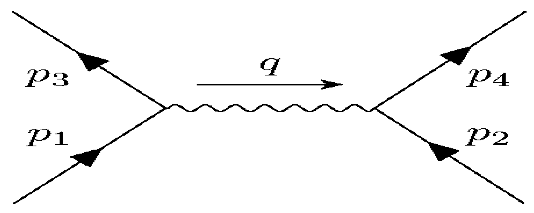
NRL of Electrodynamics

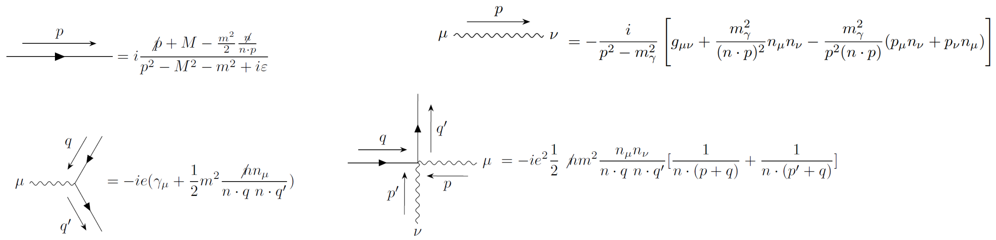
We now consider $e-e$ scattering at the tree level, using the Feynman rules of Appendix A. It is given by Figure 1:

Thus:

$$\begin{array}{cc}\hfill i\mathcal{M}={(-ie)}^2{\overline{u}}_3\left({\gamma }^{\mu }+{\displaystyle \frac{1}{2}}{m}^2{\displaystyle \frac{\cancel{n}{n}^{\mu }}{n·p_{1}n·p_3}}\right)u_1{\Delta }_{\mu \nu }(q){\overline{u}}_4\left({\gamma }^{\nu }+{\displaystyle \frac{1}{2}}{m}^2{\displaystyle \frac{\cancel{n}{n}^{\nu }}{n·p_{2}n·p_4}}\right)u_2,& q=p_1-p_3\end{array}$$

But the external legs are on-shell, so

$$\begin{array}{cc}\hfill q_{\mu }{\overline{u}}_3\left({\gamma }^{\mu }+{\displaystyle \frac{1}{2}}{m}^2{\displaystyle \frac{\cancel{n}{n}^{\mu }}{n·p_{1}n·p_3}}\right)u_1=0,& q_{\nu }{\overline{u}}_4\left({\gamma }^{\nu }+{\displaystyle \frac{1}{2}}{m}^2{\displaystyle \frac{\cancel{n}{n}_{\nu }}{n·p_{2}n·p_4}}\right)u_2=0\end{array}$$

Also:

$$\begin{array}{ccc}\hfill {\overline{u}}_3\left({\gamma }^{\mu }+{\displaystyle \frac{1}{2}}{m}^2{\displaystyle \frac{\cancel{n}{n}^{\mu }}{n·p_{1}n·p_3}}\right)u_1{n}_{\mu }{n}_{\nu }{\overline{u}}_4\left({\gamma }^{\nu }+{\displaystyle \frac{1}{2}}{m}^2{\displaystyle \frac{\cancel{n}{n}_{\nu }}{n·p_{2}n·p_4}}\right)u_2=& & \\ \hfill {\overline{u}}_3\cancel{n}{u}_1{\overline{u}}_4\cancel{n}{u}_2& \end{array}$$

In the NRL, we have

$$\begin{array}{ccc}\hfill {\overline{u}}_3\cancel{n}{u}_1=2n_{0}M{\delta }_{s_1{s}_3}& & \\ \hfill {\overline{u}}_3{\gamma }^{\mu }{u}_1=2M{\delta }_{s_1{s}_3}{\delta }_0^{\mu }& \end{array}$$

That is:

$$\begin{array}{ccc}\hfill i\mathcal{M}=i{e}^2{(2M)}^2{\displaystyle \frac{1}{q^2-m_{\gamma }^2}}{\delta }_{s_1{s}_3}{\delta }_{s_2{s}_4}\left(1+{\displaystyle \frac{n_0^2{m}_{\gamma }^2}{{(n·q)}^2}}\right),& & q=(0,\overrightarrow{q})\hfill \end{array}$$

Compare with the Born approximation

$$\begin{array}{ccc}\hfill <p^{\prime }\left|iT\right|p>& =-i\overline{V}(\overrightarrow{q})2\pi \delta (E_{p^{\prime }}-E_p),& \overrightarrow{q}={\overrightarrow{p}}^{\prime }-\overrightarrow{p}\hfill \end{array}$$

$$\begin{array}{cc}\hfill \overline{V}(\overrightarrow{q})={\displaystyle \frac{e^2}{{\overrightarrow{q}}^2+m_{\gamma }^2}}\left(1+{\displaystyle \frac{m_{\gamma }^2}{{(\widehat{n}.\overrightarrow{q})}^2}}\right)& \end{array}$$

$$\begin{array}{cc}\hfill V(\overrightarrow{x})=e^2\int {\displaystyle \frac{d^{3}q}{{(2\pi )}^3}}{\displaystyle \frac{e^{i\overrightarrow{q}.\overrightarrow{x}}}{{\overrightarrow{q}}^2+m_{\gamma }^2}}\left(1+{\displaystyle \frac{m_{\gamma }^2}{{(\widehat{n}.\overrightarrow{q})}^2}}\right)& \end{array}$$

The first term produced the expected Yukawa potential:

$$\begin{array}{cc}\hfill V(\overrightarrow{x})={\displaystyle \frac{e^2}{4\pi }}{\displaystyle \frac{e^{-m_{\gamma }r}}{r}}+e^2\int {\displaystyle \frac{d^{3}q}{{(2\pi )}^3}}{\displaystyle \frac{e^{i\overrightarrow{q}.\overrightarrow{x}}}{{\overrightarrow{q}}^2+m_{\gamma }^2}}{\displaystyle \frac{m_{\gamma }^2}{{(\widehat{n}.\overrightarrow{q})}^2}}& \end{array}$$

The second term is infrared divergent and needs to be regularized. But for all regularizations, the potential diverges for certain values of ${\displaystyle \frac{\overrightarrow{x}.\widehat{n}}{r}}$ for any r, which implies the existence of infinite forces for certain angles for any r, which is ruled out by experiments.

3. A New Regularization

Write:

$$\int {\displaystyle \frac{d^{3}q}{{(2\pi )}^3}}{\displaystyle \frac{e^{i\overrightarrow{q}.\overrightarrow{x}}}{{\overrightarrow{q}}^2+m_{\gamma }^2}}{\displaystyle \frac{1}{{(\widehat{n}.\overrightarrow{q})}^2}}=-n_0^2{\int }_{-\infty }^{\infty }d{x}_0\int {\displaystyle \frac{d^{4}q}{{(2\pi )}^4}}{\displaystyle \frac{e^{-iq.x}}{q^2-m_{\gamma }^2}}{\displaystyle \frac{1}{{(n·q)}^2}}$$

Compute:

$$U(x)=\int {\displaystyle \frac{d^{4}q}{{(2\pi )}^4}}{\displaystyle \frac{e^{-iq.x}}{q^2-m_{\gamma }^2}}{\displaystyle \frac{1}{{(n·q)}^2}}$$

We desire to keep gauge invariance, naive power counting, and $Sim(2)$ symmetry. The first two properties are satisfied by Mandelstam-Leibbrandt (ML) prescription [28,29]. The ML is:

$${\displaystyle \frac{1}{n·p}}=\underset{\epsilon \to 0}{lim}{\displaystyle \frac{p·\overline{n}}{n·pp·\overline{n}+i\epsilon }}$$

(2)

where ${\overline{n}}_{\mu }$ is a new null vector with the property $n·\overline{n}=1$.

ML introduces an additional null vector ${\overline{n}}_{\mu }$ that breaks the $Sim(2)$ symmetry of the model.

Nevertheless, there is a simple way to recover $Sim(2)$ symmetry: to take the limit ${\overline{n}}_{\mu }\to 0$. Then, only one null vector will remain: $n_{\mu }$.

Let us see how this limit can be implemented, using as an example, $U(x)$.

To calculate $U(x)$ from the definition of ML (Equation (2)) is complicated.

Instead, we want to point out the following symmetry:

$$n_{\mu }\to \lambda n_{\mu },{\overline{n}}_{\mu }\to {\lambda }^{-1}{\overline{n}}_{\mu },\lambda \ne 0,\lambda \epsilon R$$

(3)

It keeps the definitions of $n_{\mu }$ and ${\overline{n}}_{\mu }$:

$$\begin{array}{ccc}\hfill 0=n·n\to {\lambda }^{2}n·n=0& & \\ \hfill 0=\overline{n}·\overline{n}\to {\lambda }^{-2}\overline{n}·\overline{n}=0& & \\ \hfill 1=n·\overline{n}\to n·\overline{n}=1& \end{array}$$

We see from (2) that:

$${\displaystyle \frac{1}{n·p}}\to {\displaystyle \frac{1}{n·p}}{\lambda }^{-1}$$

$U(x)$ can be written as follows:

$$\begin{array}{ccc}\hfill U(x)=\int {\displaystyle \frac{d^{4}q}{{(2\pi )}^4}}{\displaystyle \frac{e^{-iq.x}}{q^2-m_{\gamma }^2}}{\displaystyle \frac{1}{{(n·q)}^2}}=& & \\ \hfill {(\overline{n}·x)}^{2}f(x·x,n·x\overline{n}·x)& \end{array}$$

where the function $f(x·x,n·x\overline{n}·x)$ is uniquely determined by the following conditions:

• $n·n=0=\overline{n}·\overline{n}$, $n·\overline{n}=1$
• Scale invariance under $n_{\mu }\to \lambda n_{\mu },{\overline{n}}_{\mu }\to {\lambda }^{-1}{\overline{n}}_{\mu }$.
• $f(x·x,n·x\overline{n}·x)$ must be regular at $n·x\overline{n}·x=0$.

The technique used to determine this function is explained in Ref. [30].

To obtain the limit ${\overline{n}}_{\mu }\to 0$, we use the following approach. Write ${\overline{n}}_{\mu }=\rho {\overline{n}}_{\mu }^{(0)},n_{\mu }={\rho }^{-1}{n}_{\mu }^{(0)}$, with ${\overline{n}}_{\mu }^{(0)},n_{\mu }^{(0)}$ satisfying condition 1. Then, condition 1. is satisfied for all $\rho$.

We define ${\overline{n}}_{\mu }\to 0$ by the limit $\rho \to 0$.

We obtain ${lim}_{\rho \to 0}{\rho }^2{({\overline{n}}^{(0)}·x)}^{2}f(x·x,n^{(0)}·x{\overline{n}}^{(0)}·x)=0$.

That is, due to $Sim(2)$ symmetry, we must have

$$U(x)=\int {\displaystyle \frac{d^{4}q}{{(2\pi )}^4}}{\displaystyle \frac{e^{-iq.x}}{q^2-m_{\gamma }^2}}{\displaystyle \frac{1}{{(n·q)}^2}}=0$$

Then

$$\int {\displaystyle \frac{d^{3}q}{{(2\pi )}^3}}{\displaystyle \frac{e^{i\overrightarrow{q}.\overrightarrow{x}}}{{\overrightarrow{q}}^2+m_{\gamma }^2}}{\displaystyle \frac{1}{{(\widehat{n}.\overrightarrow{q})}^2}}=0$$

Thus

$$\begin{array}{cc}\hfill V(\overrightarrow{x})={\displaystyle \frac{e^2}{4\pi }}{\displaystyle \frac{e^{-m_{\gamma }r}}{r}}& \end{array}$$

which is the expected Yukawa potential for a massive photon.

The same solution applies to the gravitational potential in very special linear gravity (VSLG) [31,32]. In VSLG, the graviton propagator contains terms similar to the massive photon propagator (Appendix A). When we use it to compute the classical gravitational potential between two masses, we obtain the same non-physical terms of the form:

$$\int {\displaystyle \frac{d^{3}q}{{(2\pi )}^3}}{\displaystyle \frac{e^{i\overrightarrow{q}.\overrightarrow{x}}}{{\overrightarrow{q}}^2+m_{\gamma }^2}}{\displaystyle \frac{1}{{(\widehat{n}.\overrightarrow{q})}^n}},n=2,4$$

The $Sim(2)$ limit of these integrals vanishes, so we recover a Yukawa-type gravitational potential.

A More General Integral

Consider an arbitrary function g and calculate

$$\int {\displaystyle \frac{d^{d}q}{{(2\pi )}^d}}g(q^2,q·x){\displaystyle \frac{1}{{(n·q)}^a}}$$

The M-L prescription using the method of [30] implies

$$\int {\displaystyle \frac{d^{d}q}{{(2\pi )}^d}}g(q^2,q·x){\displaystyle \frac{1}{{(n·q)}^a}}={(\overline{n}·x)}^{a}f(x·x,n·x\overline{n}·x)$$

for a unique $f(x·x,n·x\overline{n}·x)$, under the conditions:

• $n·n=0=\overline{n}·\overline{n}$, $n·\overline{n}=1$
• Scale invariance under $n_{\mu }\to \lambda n_{\mu },{\overline{n}}_{\mu }\to {\lambda }^{-1}{\overline{n}}_{\mu }$.
• $f(x·x,n·x\overline{n}·x)$ must be regular at $n·x\overline{n}·x=0$.

$x_{\mu }$ is an arbitrary vector.

To obtain the limit ${\overline{n}}_{\mu }\to 0$, write ${\overline{n}}_{\mu }=\rho {\overline{n}}_{\mu }^{(0)},n_{\mu }={\rho }^{-1}{n}_{\mu }^{(0)}$, with ${\overline{n}}_{\mu }^{(0)},n_{\mu }^{(0)}$ satisfying condition 1. Then condition 1. is satisfied for all $\rho$.

We define ${\overline{n}}_{\mu }\to 0$ by the limit $\rho \to 0$.

We obtain ${lim}_{\rho \to 0}{\rho }^a{({\overline{n}}^{(0)}·x)}^{a}f(x·x,n^{(0)}·x{\overline{n}}^{(0)}·x)=0$.

Thus:

$$\int {\displaystyle \frac{d^{d}q}{{(2\pi )}^d}}g(q^2,q·x){\displaystyle \frac{1}{{(n·q)}^a}}=0,a>0$$

It is clear that this result applies to loop integrals of the sort [30]:

$$\begin{array}{ccc}\hfill \int dp{\displaystyle \frac{1}{{[p^2+2p.q-m^2+i\epsilon ]}^a}}{\displaystyle \frac{1}{{(n·p)}^b}}={(-1)}^{a+b}i{(\pi )}^{\omega }{(-2)}^b{\displaystyle \frac{\Gamma (a+b-\omega )}{\Gamma (a)\Gamma (b)}}{(\overline{n}·q)}^b& & \\ \hfill {\int }_0^{1}dt{t}^{b-1}{\displaystyle \frac{1}{{(m^2+q^2-2n·q\overline{n}·qt-i\epsilon )}^{a+b-\omega }}},& \omega ={\displaystyle \frac{d}{2}}& \end{array}$$

(4)

Therefore, the $Sim(2)$ limit is:

$$\int dp{\displaystyle \frac{1}{{[p^2+2p.q-m^2+i\epsilon ]}^a}}{\displaystyle \frac{1}{{(n·p)}^b}}=0,b>0,q_{\mu }arbitrary$$

Taking derivatives in $q_{\mu }$, we obtain:

$$\int dp{\displaystyle \frac{1}{{[p^2+2p.q-m^2+i\epsilon ]}^a}}{\displaystyle \frac{p_{{\alpha }_1}\dots .p_{{\alpha }_n}}{{(n·p)}^b}}=0,b>0,q_{\mu }arbitrary$$

That is, the $Sim(2)$-invariant regularization of any integral over $p_{\mu }$, containing ${\displaystyle \frac{1}{n·p}}$ to any positive power, must be put to zero.

It is clear that this procedure respects gauge invariance and $Sim(2)$ invariance.

But what happens if $\gamma$ matrices are included?

See an example:

$$\begin{array}{cc}\hfill \int {\displaystyle \frac{dp}{p^2-m^2}}{\displaystyle \frac{\cancel{n}\cancel{p}\cancel{n}}{n·p}}=\int {\displaystyle \frac{dp}{p^2-m^2}}{\displaystyle \frac{(2n·p-\cancel{p}\cancel{n})\cancel{n}}{n·p}}=2\int {\displaystyle \frac{dp}{p^2-m^2}}& \end{array}$$

I can evaluate p integral first, using ML:

$$\begin{array}{cc}\hfill \int {\displaystyle \frac{dp}{p^2-m^2}}{\displaystyle \frac{\cancel{n}\cancel{p}\cancel{n}}{n·p}}=\cancel{n}{\gamma }_{\mu }\cancel{n}\int {\displaystyle \frac{dp}{p^2-m^2}}{\displaystyle \frac{p_{\mu }}{n·p}}=\cancel{n}{\gamma }_{\mu }\cancel{n}\int {\displaystyle \frac{dp}{p^2-m^2}}{\overline{n}}_{\mu }& \end{array}$$

the naive limit will be zero, but if we move $\cancel{n}$ to the right (or left) $\cancel{n}\overline{\cancel{n}}\cancel{n}=2$, we obtain the same answer as before.

But, assume that $\cancel{n}$ was already to the right. Consider:

$$\begin{array}{cc}\hfill \int {\displaystyle \frac{dp}{p^2-m^2}}{\displaystyle \frac{\cancel{p}\cancel{n}}{n·p}}=\int {\displaystyle \frac{dp}{p^2-m^2}}\overline{n}\cancel{n}\to ?& \end{array}$$

Prescription: We move all $\cancel{n}$ to the right, pick up all $n·(p+R)$ produced by this motion, and use them to cancel as many $n·(p+R)$ in the denominator as possible. Finally, all remaining ${(n·(p+R))}^{-a},a>0$ are replaced by zero. Here, $R_{\mu }$ represents any vector different from $p_{\mu }$ (the integration variable) including the zero vector. Notice that ${\displaystyle \frac{n·p}{n·(p+q)}}=1$ because ${\displaystyle \frac{n·p}{n·(p+q)}}=1-{\displaystyle \frac{n·q}{n·(p+q)}}$ and the second term vanishes in the last step of the procedure.

According to this:

$$\begin{array}{c}\hfill \int {\displaystyle \frac{dp}{p^2-m^2}}{\displaystyle \frac{\cancel{p}\cancel{n}}{n·p}}=0\end{array}$$

and

$$\begin{array}{cc}\hfill \int {\displaystyle \frac{dp}{p^2-m^2}}{\displaystyle \frac{\cancel{n}\cancel{p}\cancel{n}}{n·p}}=2\int {\displaystyle \frac{dp}{p^2-m^2}}& \end{array}$$

The reason behind this prescription is the following. We want ${\overline{n}}_{\mu }=0$ to recover $Sim(2)$ invariance. But we are not permitted to lose gauge invariance. Gauge invariance appears in the form of Ward identities that the Feynman graphs must satisfy. If we write all graphs in a “canonical form” such as all $\cancel{n}$ to the right in all monomials (only one $\cancel{n}$ remains because $\cancel{n}.\cancel{n}=0$), the Ward identities that generally involve products with external momenta will be satisfied for arbitrary values of $n_{\mu }$ and ${\overline{n}}_{\mu }$ (to prove the Ward identity, we do not need $n·n=\overline{n}·\overline{n}=0$, $n·\overline{n}=1$ when all $\cancel{n}$ are to the right of all $\overline{\cancel{n}}$). Then, after evaluating ${\overline{n}}_{\mu }=0$, the Ward identity still will be satisfied in the surviving set of integrals defining the graphs. This remaining set defines the $Sim(2)$-invariant gauge theory.

The prescription has a degree of arbitrariness. We could equally well use the convention of moving all $\cancel{n}$ to the left.

In the calculations in VSR QED, we have verified whether this arbitrariness in the prescription produces ambiguities. We did not find any.

In Appendix B, we present the method of traces to take the ${\overline{n}}_{\mu }=0$ limit. Using the trace method, it is obvious that the Ward identities are satisfied for the ${\overline{n}}_{\mu }=0$ sector. In VSR QED, the trace method gives the same results as the one presented in this chapter.

In the next section, we will apply this prescription to take the ${\overline{n}}_{\mu }\to 0$ limit ($Sim(2)$ limit) to VSR QED. We will see that the answer is explicitly gauge-invariant.

4. Renormalization of VSR QED

In this section, we follow [33].

Since the $U(1)$ gauge symmetry, as well as the $Sim(2)$ symmetry of the photon and electron, are preserved, the whole renormalized lagrangian of VSR QED is:

$$\begin{array}{ccc}\hfill {\mathcal{L}}_R=-{\displaystyle \frac{1}{4}}{Z}_3{F}_{\mu \nu }{F}^{\mu \nu }-{\displaystyle \frac{1}{2}}{m}_{\gamma }^2{Z}_{\gamma }(n^{\alpha }{F}_{\mu \alpha }){\displaystyle \frac{1}{{(n·\partial )}^2}}(n_{\beta }{F}^{\mu \beta })+& & \\ \hfill Z_2\overline{\psi }i\cancel{D}\psi +Z_{\nu }\overline{\psi }{\displaystyle \frac{i}{2}}\cancel{n}{m}^2{(n·D)}^{-1}\psi -Z_{0}M\overline{\psi }\psi & & \\ \hfill D_{\mu }={\partial }_{\mu }-ie{A}_{\mu }& \end{array}$$

Z’s are renormalization constants.

${\mathcal{L}}_R$ is invariant under renormalized gauge transformations:

$$\begin{array}{ccc}\hfill {\psi }^{\prime }(x)=e^{i\alpha (x)}\psi (x)& & \\ \hfill A_{\mu }^{\prime }(x)=A_{\mu }(x)+{\displaystyle \frac{1}{e}}{\partial }_{\mu }\alpha (x)\end{array}$$

In perturbation theory, we write:

$$\begin{array}{ccc}\hfill {\mathcal{L}}_R=-{\displaystyle \frac{1}{4}}{F}_{\mu \nu }{F}^{\mu \nu }-{\displaystyle \frac{1}{2}}{m}_{\gamma }^2(n^{\alpha }{F}_{\mu \alpha }){\displaystyle \frac{1}{{(n·\partial )}^2}}(n_{\beta }{F}^{\mu \beta })+& & \\ \hfill \overline{\psi }i\cancel{D}\psi +\overline{\psi }{\displaystyle \frac{i}{2}}\cancel{n}{m}^2{(n·D_R)}^{-1}\psi -M\overline{\psi }\psi +& & \\ \hfill -{\displaystyle \frac{1}{4}}(Z_3-1)F_{\mu \nu }{F}^{\mu \nu }-{\displaystyle \frac{1}{2}}{m}_{\gamma }^2(Z_{\gamma }-1)(n^{\alpha }{F}_{\mu \alpha }){\displaystyle \frac{1}{{(n·\partial )}^2}}(n_{\beta }{F}^{\mu \beta })+& & \\ \hfill (Z_2-1)\overline{\psi }i\cancel{D}\psi +(Z_{\nu }-1)\overline{\psi }{\displaystyle \frac{i}{2}}\cancel{n}{m}^2{(n·D_R)}^{-1}\psi -(Z_0-1)M\overline{\psi }\psi & \end{array}$$

and treat the counter terms involving $Z_3-1$, $Z_{\gamma }-1$, $Z_2-1$, $Z_{\nu }-1$ and $Z_0-1$ as perturbations.

4.1. Renormalized Photon Mass

Let ${\Pi }_{\mu \nu }$ be the photon self energy. ${\Pi }_{\mu \nu }$ is symmetric, $Sim(2)$-invariant, and satisfies the Ward identity $p_{\mu }{\Pi }_{\mu \nu }=0$. Therefore:

$${\Pi }_{\mu \nu }=A_2(p_{\mu }{p}_{\nu }-p^2{\eta }_{\mu \nu })+A_3\left({\displaystyle \frac{p_{\mu }{n}_{\nu }+p_{\nu }{n}_{\mu }}{n·p}}-{\displaystyle \frac{p^2{n}_{\mu }{n}_{\nu }}{{(n·p)}^2}}-{\eta }_{\mu \nu }\right)$$

(5)

$Sim(2)$ invariance implies that $A_i$ is function of $p^2$ only. The inverse of the full propagators is:

$$\begin{array}{ccc}\hfill {\Delta }_{\mu \nu }^{-1}=-(-p^2+m_{\gamma }^2){\eta }_{\mu \nu }-m_{\gamma }^2{\displaystyle \frac{p^2}{{(n·p)}^2}}{n}_{\mu }{n}_{\nu }+m_{\gamma }^2{\displaystyle \frac{n_{\mu }{p}_{\nu }+n_{\nu }{p}_{\mu }}{n·p}}-{\Pi }_{\mu \nu }=& & \\ \hfill {\eta }_{\mu \nu }(p^2-m_{\gamma }^2+p^2{A}_2+A_3)-A_2{p}_{\mu }{p}_{\nu }+{\displaystyle \frac{n_{\mu }{p}_{\nu }+n_{\nu }{p}_{\mu }}{n·p}}(m_{\gamma }^2-A_3)+{\displaystyle \frac{p^2}{{(n·p)}^2}}{n}_{\mu }{n}_{\nu }(A_3-m_{\gamma }^2)& \end{array}$$

The full propagator is:

$$\begin{array}{c}\hfill {\Delta }_{\mu \nu }={\displaystyle \frac{A_2}{(A_2+1){(p^2)}^2}}{p}_{\mu }{p}_{\nu }+{\displaystyle \frac{1}{p^2-m_{\gamma }^2+p^2{A}_2+A_3}}\\ \hfill \left({\eta }_{\mu \nu }+{\displaystyle \frac{n_{\mu }{p}_{\nu }+n_{\nu }{p}_{\mu }}{n·p}}\left({\displaystyle \frac{A_3-m_{\gamma }^2}{p^2(A_2+1)}}\right)-{\displaystyle \frac{p^2}{{(n·p)}^2}}{n}_{\mu }{n}_{\nu }\left({\displaystyle \frac{A_3-m_{\gamma }^2}{p^2(A_2+1)}}\right)\right)\end{array}$$

It is easy to check that the longitudinal part of the full propagator does not obtain radiative corrections, which is required by the Ward identity.

The full propagator have a pole at $p^2=m_R^2$ ($m_R$ is the physical photon mass) when

$$m_{\gamma }^2=m_R^2(1+(A_2(m_R^2)+(Z_3-1)))+(A_3(m_R^2)+(Z_{\gamma }-1)m_{\gamma }^2)$$

(6)

Around the pole:

$$\begin{array}{ccc}\hfill {\Delta }_{\mu \nu }\sim z_{\gamma }^{-1}{\displaystyle \frac{1}{p^2-m_R^2}}\left({\eta }_{\mu \nu }-{\displaystyle \frac{n_{\mu }{p}_{\nu }+n_{\nu }{p}_{\mu }}{n·p}}+{\displaystyle \frac{p^2}{{(n·p)}^2}}{n}_{\mu }{n}_{\nu }\right)& & \\ \hfill z_{\gamma }^{-1}=1+(A_2(m_R^2)+(Z_3-1))+m_R^2{A}_2^{\prime }(m_R^2)+A_3^{\prime }(m_R^2)& \end{array}$$

$z_{\gamma }$ is photon’s wave function renormalization.

4.2. Renormalized Electron Mass

Let $\Sigma (p)$ be the electron self energy. Write:

$$\begin{array}{cc}\hfill \Sigma (p)=A(p^2)\cancel{p}+B(p^2){\displaystyle \frac{\cancel{n}}{n·p}}+C(p^2)& \end{array}$$

The inverse of the full propagator is:

$$\begin{array}{ccc}\hfill S^{-1}=\cancel{p}-M-{\displaystyle \frac{m^2}{2}}{\displaystyle \frac{\cancel{n}}{n·p}}-\Sigma (p)=& & \\ \hfill (1-A)\left(\cancel{p}-{\displaystyle \frac{{\overline{m}}^2}{2}}{\displaystyle \frac{\cancel{n}}{n·p}}-\overline{M}\right)& & \\ \hfill {\overline{m}}^2={\displaystyle \frac{m^2+2B(p^2)}{1-A(p^2)}},\overline{M}={\displaystyle \frac{M+C(p^2)}{1-A(p^2)}}& \end{array}$$

Then:

$$\begin{array}{ccc}\hfill S={\displaystyle \frac{1}{1-A(p^2)}}{\displaystyle \frac{\left(\cancel{p}-\frac{{\overline{m}}^2}{2}\frac{\cancel{n}}{n·p}+\overline{M}\right)}{p^2-{\overline{m}}^2(p^2)-{\overline{M}}^2(p^2)}}=& & \\ \hfill {\displaystyle \frac{\left(\cancel{p}-\frac{{\overline{m}}^2}{2}\frac{\cancel{n}}{n·p}+\overline{M}\right)}{p^2(1-A(p^2))-m^2-2B(p^2)-\frac{{(M+C(p^2))}^2}{1-A(p^2)}}}& & \end{array}$$

(7)

It has a pole when:

$$\begin{array}{cc}\hfill p^2={\overline{m}}^2(M_R^2)+{\overline{M}}^2(M_R^2)=M_R^2& \end{array}$$

(8)

Define

$K=p^2(1-A(p^2))-m^2-2B(p^2)-{\displaystyle \frac{{(M+C(p^2))}^2}{1-A(p^2)}}$

The residue at the pole $p^2=M_R^2$ is

$$\begin{array}{c}\hfill z_e^{-1}=K^{\prime }(M_R^2)=1-A(M_R^2)-M_R^2{A}^{\prime }(M_R^2)-2B^{\prime }(M_R^2)-\\ \hfill (2\overline{M}(M_R^2)C^{\prime }(M_R^2)+A^{\prime }(M_R^2)\overline{M}{(M_R^2)}^2)& \end{array}$$

Introduce the notation $Q(M_R^2)=\overline{Q}$. Then, in perturbation theory:

$$\begin{array}{cc}\hfill z_e=1+\overline{A}+M_R^2{\overline{A}}^{\prime }+2{\overline{B}}^{\prime }+2M{\overline{C}}^{\prime }+{\overline{A}}^{\prime }{M}^2+\dots & \end{array}$$

$z_e$ is the electron’s wave function renormalization.

5. Single-Loop VSR QED with a Gauge-Invariant Photon Mass

In this section, we apply our $Sim(2)$ regularization, ${\overline{n}}_{\mu }=0$ limit, to obtain the renormalized single-particle irreducible graphs at one loop in VSR QED with a gauge-invariant photon mass. Most of the computations have used FORM [34].

We will verify that the Ward identity for the photon self energy is preserved and that the Ward–Takahashi identity is satisfied. We will explicitly calculate the counter terms in the on-shell renormalization scheme (OSR). All along, the $Sim(2)$ symmetry is respected.

Finally, the on-shell $\gamma -e-e$ vertex is evaluated. We verified that the renormalized vertex is conserved in the OSR. To show this is non-trivial. The gauge and $Sim(2)$ symmetry play a fundamental role.

Having carried this out, we were able to obtain a prediction for the anomalous magnetic moment of the electron, taking into account a massive neutrino and a gauge-invariant photon mass, $m_{\gamma }$. It has log corrections in $m_{\gamma }$, which means that the model does not reduce to the one without a photon mass in the zero photon mass limit. These log corrections are actually interesting from the phenomenological point of view because they enhance the very small contribution of the neutrino mass to the anomalous magnetic moment of the electron.

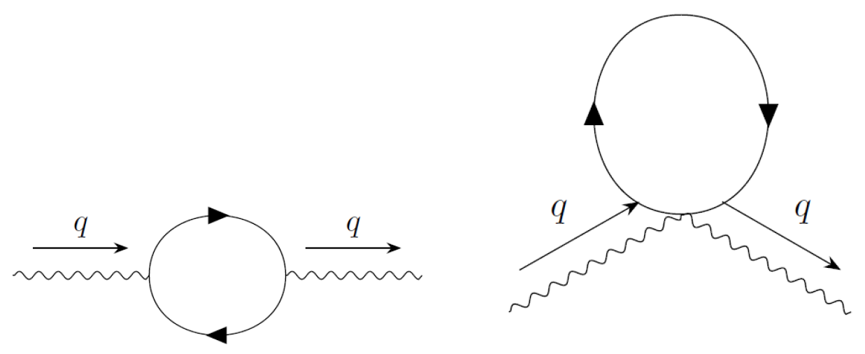
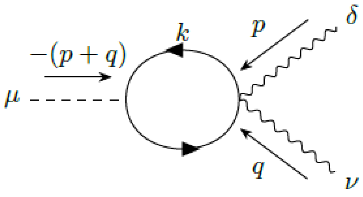
5.1. Photon Self Energy

In this subsection, we present the calculation of the photon self-energy. It is given by the two graphs of Figure 2:

$$\begin{array}{ccc}\hfill i{\Pi }_{1\mu \nu }=-{(-ie)}^2\int dpTr(\left[{\gamma }_{\mu }+{\displaystyle \frac{1}{2}}{\displaystyle \frac{n_{\mu }\cancel{n}{m}^2}{n·(p+q)n·p}}\right]{\displaystyle \frac{i\left(\cancel{p}+M-\frac{m^2}{2}\frac{\cancel{n}}{n·p}\right)}{p^2-M_e^2+i\epsilon }}& & \\ \hfill \left[{\gamma }_{\nu }+{\displaystyle \frac{1}{2}}{\displaystyle \frac{n_{\nu }\cancel{n}{m}^2}{n·(p+q)n·p}}\right]{\displaystyle \frac{i\left(\cancel{p}+\cancel{q}+M-\frac{m^2}{2}\frac{\cancel{n}}{n·(p+q)}\right)}{{(p+q)}^2-M_e^2+i\epsilon }})& \end{array}$$

(9)

$$\begin{array}{cc}\hfill i{\Pi }_{2\mu \nu }=e^{2}i{n}_{\mu }{n}_{\nu }\int dp{\displaystyle \frac{1}{n·pn·(p+q)n·(p-q)}}Tr(\cancel{n}{m}^2{\displaystyle \frac{i\left(\cancel{p}+M-\frac{m^2}{2}\frac{\cancel{n}}{n·p}\right)}{p^2-M_e^2+i\epsilon }})& \end{array}$$

(10)

We use the new prescription to compute the diagrams. The second graph vanishes in the $Sim(2)$ limit, whereas the first graph is:

$$\begin{array}{cc}\hfill i{\Pi }_{\mu \nu }=4e^2\int {\displaystyle \frac{d^{d}p}{{(2\pi )}^d}}{\displaystyle \frac{-2p_{\mu }{p}_{\nu }-p_{\mu }{q}_{\nu }-p_{\nu }{q}_{\mu }-{\eta }_{\mu \nu }(M_e^2-p^2-p.q)}{(p^2-M_e^2+i\epsilon )({(p+q)}^2-M_e^2+i\epsilon )}}& \end{array}$$

Notice that some terms proportional to $m^2$ survive. They come from terms produced by the trace of the sort: $m^{2}n·p,m^{2}n·(p+q)$. These terms cancel the ${\displaystyle \frac{1}{n·p}},{\displaystyle \frac{1}{n·(p+q)}}$, so that after applying the $Sim(2)$ limit, they survive. These are just the terms we need to write the final result entirely in terms of the physical electron mass, $M_e^2=M^2+m^2$, which is expected from unitarity.

We obtain the standard QED result, with the electron mass $M_e=\sqrt{M^2+m^2}$.

Write:

$$\begin{array}{cc}\hfill {\eta }^{\mu \nu }{\Pi }_{\mu \nu }(q)=(d-1)q^2\Pi (q)& \end{array}$$

Then:

$$\begin{array}{cc}\hfill (d-1)q^2\Pi (q)=-4i{e}^2\int {\displaystyle \frac{d^{d}p}{{(2\pi )}^d}}{\displaystyle \frac{-2p^2-2p·q-d(M_e^2-p^2-p·q)}{(p^2-M_e^2+iϵ)({(p+q)}^2-M_e^2+iϵ)}}& \end{array}$$

Define $d=4-ϵ,e\to e{\mu }^{{\displaystyle \frac{ϵ}{2}}}$

$$\begin{array}{c}\hfill \Pi (q^2)=-{\displaystyle \frac{\alpha }{\pi }}\left[{\displaystyle \frac{1}{\epsilon }}{\displaystyle \frac{2}{3}}+\left({\displaystyle \frac{1}{3}}log(4\pi )-\gamma \right)-{\int }_0^{1}dx2x(1-x)log\left({\displaystyle \frac{M_e^2-x(1-x)q^2-i\epsilon }{{\mu }^2}}\right)\right]+\\ \hfill o(\epsilon )\end{array}$$

where $\alpha ={\displaystyle \frac{e^2}{4\pi }}$ is the fine structure constant.

In on-shell renormalization, we require that $m_{\gamma }=m_R$ and $z_{\gamma }=1$. We obtain two conditions:

$$\begin{array}{ccc}\hfill -\Pi (m_{\gamma }^2)+Z_3-1+Z_{\gamma }-1=0& & \\ \hfill -\Pi (m_{\gamma }^2)+Z_3-1-m_{\gamma }^2{\Pi }^{\prime }(m_{\gamma }^2)=0& \end{array}$$

$$\begin{array}{cc}\hfill Z_{\gamma }-1=m_{\gamma }^2{\Pi }^{\prime }(m_{\gamma }^2)=-2{\lambda }^2{\displaystyle \frac{\alpha }{\pi }}{\int }_0^{1}dx{\displaystyle \frac{x^2{(1-x)}^2}{1-x(1-x){\lambda }^2-i\epsilon }},& \lambda ={\displaystyle \frac{m_{\gamma }}{M_e}}\end{array}$$

a finite counter term.

$$\begin{array}{ccc}\hfill Z_3-1=-{\displaystyle \frac{\alpha }{\pi }}\left[{\displaystyle \frac{1}{\epsilon }}{\displaystyle \frac{2}{3}}+\left({\displaystyle \frac{1}{3}}log(4\pi )-\gamma \right)-{\int }_0^{1}dx2x(1-x)log\left({\displaystyle \frac{M_e^2-x(1-x)m_{\gamma }^2-i\epsilon }{{\mu }^2}}\right)\right]& & \\ \hfill -2{\lambda }^2{\displaystyle \frac{\alpha }{\pi }}{\int }_0^{1}dx{\displaystyle \frac{x^2{(1-x)}^2}{1-x(1-x){\lambda }^2-i\epsilon }}& \end{array}$$

$$\begin{array}{c}\hfill {\Pi }_{OSR}(q^2)={\displaystyle \frac{\alpha }{\pi }}\left[{\int }_0^{1}dx2x(1-x)log\left({\displaystyle \frac{M_e^2-x(1-x)q^2-i\epsilon }{M_e^2-x(1-x)m_{\gamma }^2-i\epsilon }}\right)\right]+\\ \hfill 2{\lambda }^2{\displaystyle \frac{\alpha }{\pi }}{\int }_0^{1}dx{\displaystyle \frac{x^2{(1-x)}^2}{1-x(1-x){\lambda }^2-i\epsilon }}\end{array}$$

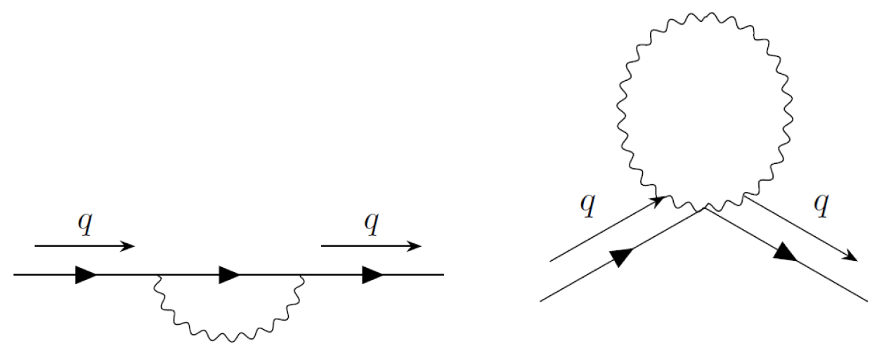
5.2. Electron Self Energy

In this subsection, we obtain the electron self-energy. We have two graphs contributing to the two proper vertexes. See Figure 3.

$$\begin{array}{ccc}\hfill -i{\Sigma }_1(q)={(-ie)}^2\int dp\left({\gamma }_{\mu }+{\displaystyle \frac{1}{2}}{m}^2\cancel{n}{n}_{\mu }{\displaystyle \frac{1}{n·(p+q)}}{\displaystyle \frac{1}{n·q}}\right){\displaystyle \frac{i\left(\cancel{p}+\cancel{q}+M-\frac{m^2}{2}\frac{\cancel{n}}{n·(p+q)}\right)}{{(p+q)}^2-M_e^2+iϵ}}& & \\ \hfill \left({\gamma }_{\nu }+{\displaystyle \frac{1}{2}}{m}^2\cancel{n}{n}_{\nu }{\displaystyle \frac{1}{n·(p+q)}}{\displaystyle \frac{1}{n·q}}\right)\left(-{\displaystyle \frac{n_{\mu }}{n·p}}{\displaystyle \frac{n_{\nu }}{n·p}}{\displaystyle \frac{i{m}_{\gamma }^2}{p^2-m_{\gamma }^2}}+{\displaystyle \frac{n_{\mu }{p}_{\nu }+n_{\nu }{p}_{\mu }}{n·p(p^2-m_{\gamma }^2)}}{\displaystyle \frac{i{m}_{\gamma }^2}{p^2}}-{\displaystyle \frac{i{\eta }_{\mu \nu }}{p^2-m_{\gamma }^2}}\right)& \end{array}$$

(11)

According to our prescription, we pass all $\cancel{n}$ to the right, pick up all $n·(p+R)$ obtained by this motion, and with them, cancel as many $n·(p+R)$ in the denominator as possible. Finally, all ${(n·(p+R))}^{-a},a>0$ that remain are replaced by zero. Here, $R_{\mu }$ represents any vector different from $p_{\mu }$ (the integration variable) including the zero vector. See that ${\displaystyle \frac{n·p}{n·(p+q)}}=1$ because ${\displaystyle \frac{n·p}{n·(p+q)}}=1-{\displaystyle \frac{n·q}{n·(p+q)}}$.

In the $Sim(2)$ limit, we obtain:

$$\begin{array}{ccc}\hfill {\Sigma }_1(p)=i{e}^{2}2m^2{\displaystyle \frac{\cancel{n}}{n·p}}(S_3-m_{\gamma }^2{I}_3)+((2-d)(V_6+S_3)+2m_{\gamma }^2{I}_3)\cancel{p}+M(d{S}_3-2m_{\gamma }^2{I}_3)& & \\ \hfill +(Z_2-1)\cancel{p}+(Z_{\nu }-1){\displaystyle \frac{1}{2}}{m}^2{\displaystyle \frac{\cancel{n}}{n·p}}-(Z_0-1)M& \end{array}$$

The functions used in this subsection are defined in Appendix C.

Thus:

$$\begin{array}{ccc}\hfill A=(2-d)(V_6+S_3)+2m_{\gamma }^2{I}_3+(Z_2-1)& & \\ \hfill B=2m^2(S_3-m_{\gamma }^2{I}_3)+(Z_{\nu }-1){\displaystyle \frac{1}{2}}{m}^2& & \\ \hfill C=M(d{S}_3-2m_{\gamma }^2{I}_3)-(Z_0-1)M& \end{array}$$

On-shell renormalization means the following:. m: physical neutrino mass; $M_e^2=M^2+m^2$: physical electron mass. That is:

$$\begin{array}{ccc}\hfill {\overline{m}}^2(M_e^2)=m^2,& 2B(M_e^2)+m^{2}A(M_e^2)=0& \\ \hfill {\overline{M}}_R(M_e^2)=M,& C(M_e^2)+A(M_e^2)M=0\end{array}$$

Moreover, we must have:

$$\begin{array}{ccc}\hfill z_e=1& & \\ \hfill A(M_e^2)+m^2{A}^{\prime }(M_e^2)+2B^{\prime }(M_e^2)+2M{C}^{\prime }(M_e^2)+2A^{\prime }(M_e^2)M^2=0& \end{array}$$

These three conditions fix the three counter terms as the pole and finite part of the ensuing expressions when $d\to 4$:

$$\begin{array}{c}{Z}_2-1=(2-d)(V_6(M_e^2)+S_3(M_e^2))-2m_{\gamma }^2{I}_3(M_e^2)-(2B^{\prime }(M_e^2)+m^2{A}^{\prime }(M_e^2)+\\ 2M{C}^{\prime }(M_e^2)+2M^2{A}^{\prime }(M_e^2))\\ Z_{\nu }-1={\displaystyle \frac{1}{m^2}}(2B^{\prime }(M_e^2)+m^2{A}^{\prime }(M_e^2)+2M{C}^{\prime }(M_e^2)+2M^2{A}^{\prime }(M_e^2))\\ -4(S_3(M_e^2)-m_{\gamma }^2{I}_3(M_e^2))\\ Z_0-1=4S_3(M_e^2)-2m_{\gamma }^2{I}_3(M_e^2)-{\displaystyle \frac{1}{M}}(2B^{\prime }(M_e^2)+m^2{A}^{\prime }(M_e^2)+2M{C}^{\prime }(M_e^2)+\\ 2M^2{A}^{\prime }(M_e^2))\end{array}$$

In the calculation of the on-shell three vertexes, we use on-shell renormalization of the electron self energy.

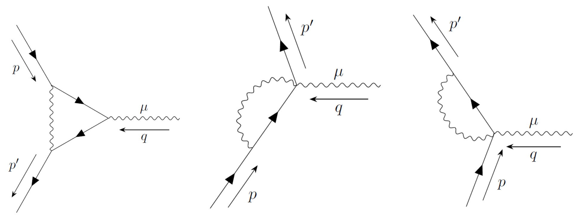
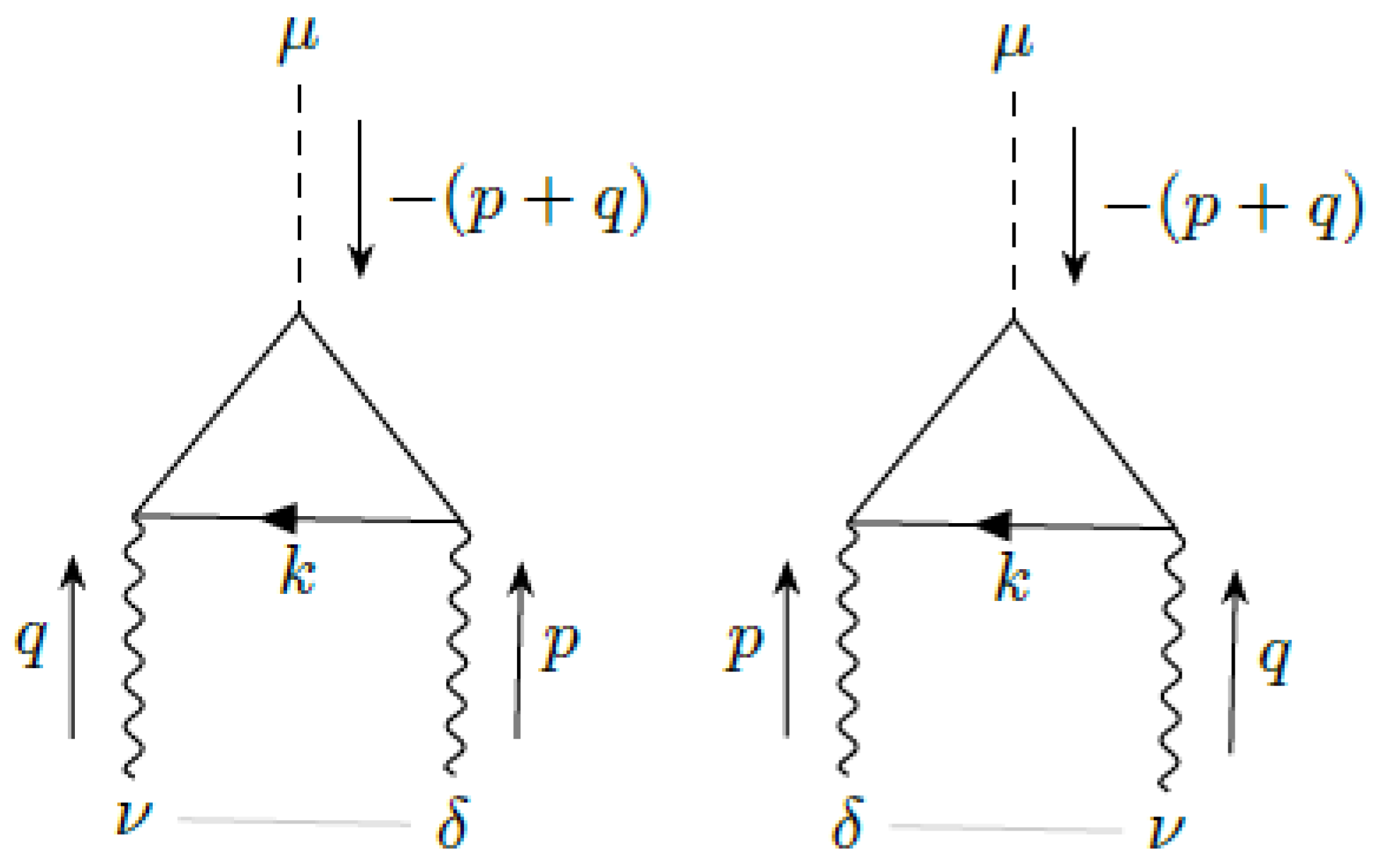
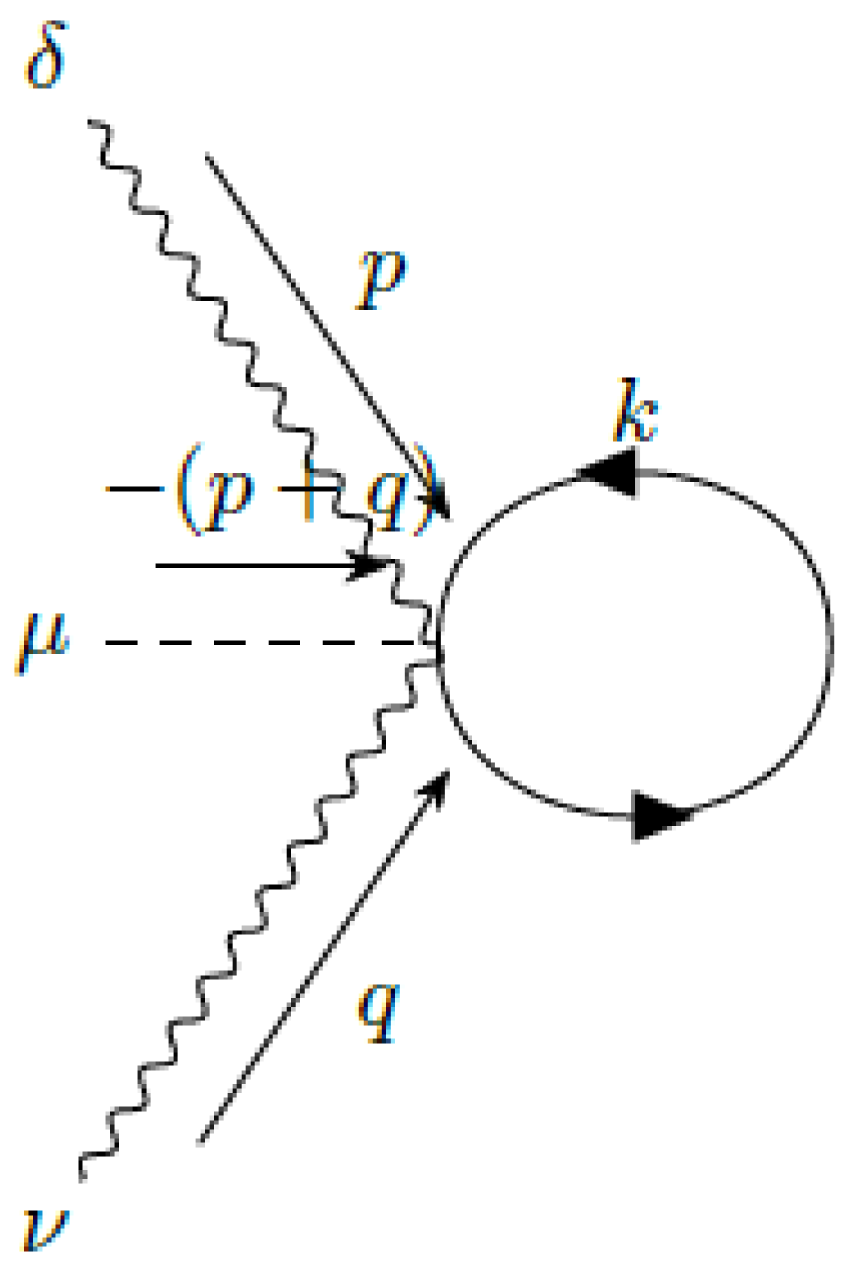
5.3. On-Shell Vertex Correction

In this subsection, we discuss the three-point proper vertex and verify the Ward–Takahashi identity. This is an important test of the gauge invariance of the infrared regulator. The single-loop contribution to ${\Gamma }^{\mu }(p^{\prime }=p+q,p)$ consists of the addition of three graphs (Figure 4):

The addition of the three graphs gives the vertex correction:

$$\begin{array}{ccc}\hfill \delta {\Gamma }^{\mu }(p+q,p)=\int dk{\displaystyle \frac{i}{{(k-p)}^2}}{(-ie)}^2\left[{\gamma }_{\nu }+{\displaystyle \frac{1}{2}}{m}^2{\displaystyle \frac{n_{\nu }\cancel{n}}{n·(p+q)n·(k+q)}}\right]{\displaystyle \frac{\left({\cancel{k}}^{\prime }+M-\frac{m^2}{2}\frac{\cancel{n}}{n·k^{\prime }}\right)}{k^{\prime 2}-M_e^2+i\epsilon }}& & \\ \hfill \left[{\gamma }^{\mu }+{\displaystyle \frac{1}{2}}{m}^2{\displaystyle \frac{n^{\mu }\cancel{n}}{n·(k+q)n·k}}\right]{\displaystyle \frac{\left(\cancel{k}+M-\frac{m^2}{2}\frac{\cancel{n}}{n·k}\right)}{k^2-M_e^2+i\epsilon }}\left[{\gamma }^{\nu }+{\displaystyle \frac{1}{2}}{m}^2{\displaystyle \frac{n^{\nu }\cancel{n}}{n·pn·k}}\right]+& & \\ \hfill {(-ie)}^2{m}^2\int dk{\displaystyle \frac{i}{{(k-p-q)}^2}}{\displaystyle \frac{1}{k^2-M_e^2+i\epsilon }}{\displaystyle \frac{n^{\mu }\cancel{n}n·(k+p)}{n·pn·(p+q)n·(k-q)}}+& & \\ \hfill {(-ie)}^2{m}^2\int dk{\displaystyle \frac{i}{{(k-p)}^2}}{\displaystyle \frac{n^{\mu }\cancel{n}n·(k+p+q)}{n·pn·(p+q)n·(k+q)}}& & \end{array}$$

(12)

Here, $k^{\prime }=k+q$. This vertex correction formally satisfies the Ward–Takahashi identity:

$$-i{q}_{\mu }{\Gamma }^{\mu }(p+q,p)=S^{-1}(p+q)-S^{-1}(p)=-i\left(\cancel{p}+\cancel{q}-M-\Sigma (p+q)-\cancel{p}+M+\Sigma (p)\right)$$

(13)

Evaluating the ${\overline{n}}_{\mu }=0$ limit we obtain our result for the vertex correction. It is written in detail in Appendix D. It is well defined, because the integrals have been dimensionally regularized. We have verified that it satisfies the Ward–Takahashi identity for any value of the parameters, including the non-zero photon mass $m_{\gamma }$. This is a remarkable result of our prescription for the VSR integrals. For the first time, we are able to incorporate a gauge-invariant photon mass that preserves explicitly all the symmetries of the model.

Now, we proceed to evaluate the on-shell vertex correction, i.e.,

$$\begin{array}{c}\hfill \overline{u}(p+q))\delta {\Gamma }^{\mu }u(p)\end{array}$$

(14)

with

$$\begin{array}{c}\hfill \left(\cancel{p}-M-{\displaystyle \frac{m^2}{2}}{\displaystyle \frac{\cancel{n}}{n·p}}\right)u(p)=0\end{array}$$

(15)

$$\begin{array}{c}\hfill \overline{u}(p+q))\left(\cancel{p}+\cancel{q}-M-{\displaystyle \frac{m^2}{2}}{\displaystyle \frac{\cancel{n}}{n·p+n·q}}\right)=0\end{array}$$

(16)

We have defined the form factors $G_2,G_3,F_3,F_1,F_2$.

$$\begin{array}{c}\hfill \overline{u}(p+q)\delta {\Gamma }^{\mu }(p+q,p)u(p)=R_{1\mu }+R_{2\mu }+\\ \hfill \overline{u}(p+q)\left\{G_2\left[-i{\sigma }^{\mu \nu }{q}_{\nu }\cancel{n}\right]+G_3\cancel{n}{Q}^{\mu }+F_3\cancel{n}{\sigma }^{\mu \nu }{q}_{\nu }\cancel{n}+{\tilde{\gamma }}^{\mu }{F}_1+F_{2}i{\displaystyle \frac{{\sigma }^{\mu \nu }}{2M}}{q}_{\nu }\right\}u(p)\end{array}$$

(17)

where

$$\begin{array}{cc}\hfill Q_{\mu }=q_{\mu }-q^2{\displaystyle \frac{n_{\mu }}{n·q}},& q·Q=0,\end{array}$$

(18)

$$\begin{array}{c}\hfill {\tilde{\gamma }}^{\mu }={\gamma }^{\mu }+{\displaystyle \frac{m^2}{2}}{\displaystyle \frac{\cancel{n}{n}^{\mu }}{n·p(n·p+n·q)}},{\tilde{\gamma }}^{\mu }{q}_{\mu }=0,onshell\end{array}$$

(19)

$$\begin{array}{c}\hfill G_3={\displaystyle \frac{i{m}^{2}n·q}{n·p(n·p+n·q)}}((2-d){\overline{T}}_8-(2-d){\overline{T}}_7+{\displaystyle \frac{{\overline{T}}_6(1-\frac{d}{2})}{2}}+(2-d){\overline{V}}_4+{\displaystyle \frac{{\overline{V}}_3(1+\frac{d}{2})}{2}})\end{array}$$

(20)

$$\begin{array}{c}\hfill F_3={\displaystyle \frac{m^{2}M}{2n·p(n·p+n·q)}}\left(\left(1-{\displaystyle \frac{d}{2}}\right){\overline{T}}_6+{\displaystyle \frac{d}{2}}{\overline{V}}_3\right)\end{array}$$

(21)

$$\begin{array}{c}\hfill G_2={\displaystyle \frac{i{m}^2}{n·p}}\left(-{\displaystyle \frac{1}{2}}\left(1-{\displaystyle \frac{d}{2}}\right){\overline{T}}_6-2{\overline{V}}_4+{\displaystyle \frac{1}{2}}\left(3-{\displaystyle \frac{d}{2}}\right){\overline{V}}_3\right)+\\ \hfill {\displaystyle \frac{i{m}^2}{n·p+n·q}}\left((d-2){\overline{T}}_7+{\displaystyle \frac{1}{2}}\left(1-{\displaystyle \frac{d}{2}}\right){\overline{T}}_6-2{\overline{V}}_4+{\displaystyle \frac{1}{2}}\left(1+{\displaystyle \frac{d}{2}}\right){\overline{V}}_3+2m_{\gamma }^2{\overline{V}}_2\right)\end{array}$$

(22)

$$\begin{array}{c}\hfill F_1=-i(2-d){\overline{V}}_6-i(8-4d){\overline{T}}_5-i(d-2){\overline{S}}_4+2i{m}_{\gamma }^2{\overline{I}}_4-i(2-d)(2M^2+m^2){\overline{T}}_6\\ \hfill -i(d-2){\displaystyle \frac{n·q}{n.(p+q)}}{m}^2{\overline{T}}_7-i(4m^2+2d{M}^2){\overline{V}}_3+4i{m}^2{\displaystyle \frac{n·p}{n.(p+q)}}{m}_{\gamma }^2{\overline{V}}_2+2i{m}^2{\displaystyle \frac{n·p}{n.(p+q)}}{m}_{\gamma }^2{\overline{S}}_1\\ \hfill -i(4-2d)q^2{\overline{T}}_8-i(2+d)q^2{\overline{T}}_7+2i{q}^2{\overline{T}}_6+Z_2-1\end{array}$$

(23)

$$\begin{array}{c}\hfill F_2=i{M}^2\left((6d-8-d^2){\overline{T}}_7+\left(8-5d+{\displaystyle \frac{d^2}{2}}\right){\overline{T}}_6+(4d-16){\overline{V}}_4+\left(5d-8-{\displaystyle \frac{d^2}{2}}\right){\overline{V}}_3\right)\end{array}$$

(24)

The two terms $R_{1\mu }$ and $R_{2\mu }$ are, in general, non-zero. We find:

$$R_{1\mu }=q_{\mu }\overline{u}(p+q)u(p)\left(2-{\displaystyle \frac{3d}{2}}+{\displaystyle \frac{d^2}{4}}\right)iM({\overline{V}}_5-{\overline{V}}_6+{\overline{S}}_4-{\overline{S}}_3)$$

(25)

which is zero on shell since ${\overline{V}}_5={\overline{V}}_6$ and ${\overline{S}}_3={\overline{S}}_4$. We recall that for integral $Q(p,q)$, we employ the notation $\overline{Q}=Q(p^2=M_e^2,q)$.

Actually $R_{1\mu }$ appears also in standard QED, so it is not a surprise that it cancels on shell.

$R_{2\mu }$ is trickier. It is not present in standard QED. It diverges in $d=4$.

$$R_{2\mu }=i\overline{u}(p+q){\displaystyle \frac{\cancel{n}{n}_{\mu }}{n·p(n·p+n·q)}}u(p)m^2(\left({\displaystyle \frac{d}{2}}-1\right){\overline{V}}_6+\left({\displaystyle \frac{d}{2}}-3\right){\overline{S}}_3+m_{\gamma }^2{\overline{I}}_3)$$

(26)

To cancel this term from the renormalized three vertex, we must add the vertex counter term. The VSR QED three vertex has two different counter terms, whereas in QED the three vertex has one counter term.

From the Lagrangian we can read the counter term for the 3-point function.

We have to find terms linear in $A_{\mu }$ in

$$\begin{array}{cc}\hfill (Z_2-1)\overline{\psi }i\cancel{D}\psi +(Z_{\nu }-1)\overline{\psi }{\displaystyle \frac{i}{2}}\cancel{n}{m}^2{(n·D)}^{-1}\psi & \end{array}$$

Thus:

$$\begin{array}{ccc}\hfill (Z_2-1){\gamma }^{\mu }-(Z_{\nu }-1){\displaystyle \frac{1}{2}}{m}^2{\displaystyle \frac{n_{\mu }\cancel{n}}{n·pn·(p+q)}}=& & \\ \hfill (Z_2-1)\left({\gamma }^{\mu }+{\displaystyle \frac{1}{2}}{m}^2{\displaystyle \frac{n_{\mu }\cancel{n}}{n·pn·(p+q)}}\right)-{\displaystyle \frac{1}{2}}{m}^2{\displaystyle \frac{n_{\mu }\cancel{n}}{n·pn·(p+q)}}((Z_{\nu }-1)+(Z_2-1))& \end{array}$$

The first counter term renormalizes the coupling of the photon to the electric current, i.e., $F_1$. The counter term that affects $R_{2\mu }$ is the last one. Due to charge conservation, the addition of the counterterm $-{\displaystyle \frac{1}{2}}{m}^2{\displaystyle \frac{n_{\mu }\cancel{n}}{n·pn·(p+q)}}((Z_{\nu }-1)+(Z_2-1))$ must cancel $R_{2\mu }$. It is easy to check that it does.

It remains to prove that on-shell renormalization implies that e is the physical electron charge. To carry this out, we must show that $F_1(q^2=0)=1$.

Let us see how it goes in VSR QED.

5.4. $F_1(0)$

Near on shell, the Ward–Takahashi identity is:

$$\begin{array}{cc}\hfill -i{k}_{\mu }{\Gamma }^{\mu }(p+k,p)=S^{-1}(p+k)-S^{-1}(p)=z_e^{-1}\left[\cancel{k}+{\displaystyle \frac{m^2}{2}}{\displaystyle \frac{\cancel{n}n·k}{{(n·p)}^2}}\right]& \end{array}$$

But the renormalization of the electric charge is:

$${\Gamma }^{\mu }(p,p)=i{F}_1(0)\left({\gamma }^{\mu }+{\displaystyle \frac{m^2}{2}}{\displaystyle \frac{\cancel{n}{n}^{\mu }}{{(n·p)}^2}}\right)$$

(27)

In the Ward–Takahashi identity:

$$\begin{array}{ccc}\hfill F_1(0)\left(\cancel{k}+{\displaystyle \frac{m^2}{2}}{\displaystyle \frac{\cancel{n}n·k}{{(n·p)}^2}}\right)=z_e^{-1}\left[\cancel{k}+{\displaystyle \frac{m^2}{2}}{\displaystyle \frac{\cancel{n}n·k}{{(n·p)}^2}}\right]& & \\ \hfill F_1(0)=z_e^{-1}\end{array}$$

Using various identities that we list in Appendix E, we are able to show that this equality holds in our infrared (${\overline{n}}^{\mu }=0$ limit) and ultraviolet (dimensional regularization) regularization. But on-shell renormalization of the electron propagator imposes $z_e=1$. Therefore, $F_1(0)=1$ and e represent the physical electron charge.

We are ready to extract the anomalous magnetic moment of the electron in the next section.

6. Anomalous Magnetic Moment of the Electron

In the non-relativistic (NR) limit, we obtain

Table 1. In the right column, we list the form factor. In the left column, we have the NR limit of the matrix element accompanying the form factor in (17). All form factors are evaluated at $q_{\mu }=0$. Here, $A_0$ is the electric potential and $A_i$ is the vector potential. ${\phi }_{s^{\prime }}$ is a two dimensional constant vector that corresponds to the NR limit of the Dirac spinors.

NR Limit	Form Factor
$2M_e{\phi }_s^{\uparrow }{\phi }_s{A}_0$	$F_1$(0)
${\displaystyle \frac{3m^2}{4M^2}}i{\epsilon }_{ijk}{\phi }_s^{\uparrow }{\sigma }^i{\phi }_{s^{\prime }}{\widehat{n}}_j{q}_k{A}_0$	$F_1$(0)
$i{\epsilon }_{ijk}{q}_j{\phi }_s^{\uparrow }{\sigma }^k{\phi }_{s^{\prime }}{A}_i$	$F_1$(0)
$-2i{n}_{0}M{\epsilon }_{ijk}{\phi }_s^{\uparrow }{\sigma }^k{\phi }_{s^{\prime }}{q}_j{A}_i$	$G_2(0)$
$-i{\epsilon }_{ijk}{n}_k{\displaystyle \frac{m^2}{M}}{\phi }_s^{\uparrow }\widehat{n}.\overrightarrow{\sigma }{\phi }_{s^{\prime }}{q}_j{A}_i$	$G_2(0)$
$i(2M{\epsilon }_{ijk}{n}_k{\phi }_s^{\uparrow }{\sigma }^j{\phi }_{s^{\prime }}+2M_{e}i{n}_i{\phi }_s^{\uparrow }{\phi }_{s^{\prime }})A_0{q}_i$	$G_2(0)$
$2M_e{n}_0{\phi }_s^{\uparrow }{\phi }_{s^{\prime }}{Q}_{\mu }{A}^{\mu }$	$G_3(0)$
$(-4M_e{\epsilon }_{ijk}{n}_k{\phi }_s^{\uparrow }\overrightarrow{n}.\overrightarrow{\sigma }{\phi }_{s^{\prime }}+4M_e{n}_0^2{\epsilon }_{ijk}{\phi }_s^{\uparrow }{\sigma }^k{\phi }_{s^{\prime }})q_j{A}_i$	$F_3(0)$
$4M_e{n}_0{\epsilon }_{ijk}{n}_j{\phi }_s^{\uparrow }{\sigma }^k{\phi }_{s^{\prime }}{A}_0{q}_i$	$F_3(0)$
$i{\epsilon }_{ijk}{\phi }_s^{\uparrow }{\sigma }^k{\phi }_{s^{\prime }}{A}_i{q}_j$	$F_2(0)$
$-i{\displaystyle \frac{m^2}{2M^2}}{\epsilon }_{ijk}{\widehat{n}}_j{\phi }_s^{\uparrow }{\sigma }^k{\phi }_s{A}_0{q}_j$	$F_2(0)$

, keeping terms that are at most linear in $q_{\mu }$.

We see that the anomalous magnetic moment is:

$$a_e=F_2(0)-2n_{0}M{G}_2(0)-4i{M}_e{n}_0^2{F}_3(0)$$

(28)

The integrals we used to calculate the form factors are listed in Appendix F. ∼ means a small $\lambda$ limit. We obtain:

$$\begin{array}{c}\hfill F_2(0)=i4M^2({\overline{V}}_3(0)-{\overline{T}}_6(0))\sim {\displaystyle \frac{\alpha }{2\pi }}{\displaystyle \frac{M^2}{M_e^2}}\end{array}$$

(29)

$$\begin{array}{c}\hfill G_2(0)=i{m}^2{\displaystyle \frac{1}{n·p}}(4{\overline{S}}_2(0)-2{\overline{V}}_3(0)+2{\overline{T}}_7(0)+2m_{\gamma }^2{\overline{V}}_2(0))\sim -{\displaystyle \frac{m^2}{M_e^2}}{\displaystyle \frac{\alpha }{2\pi n_0{M}_e}}\left(log(\lambda )-{\displaystyle \frac{3}{4}}\right)\end{array}$$

(30)

$$\begin{array}{c}\hfill F_3(0)=m^{2}M{\displaystyle \frac{1}{{(n·p)}^2}}\left(-{\displaystyle \frac{1}{2}}{\overline{T}}_6(0)+{\overline{V}}_3(0)\right)=i{\displaystyle \frac{m^2}{M_e^2}}{\displaystyle \frac{M}{n_0^2{M}_e^2}}{\displaystyle \frac{\alpha }{4\pi }}\left({\displaystyle \frac{1}{2}}log(\lambda )+{\displaystyle \frac{1}{4}}\right)\end{array}$$

(31)

That is:

$$a_e={\displaystyle \frac{\alpha }{2\pi }}\left(1+{\displaystyle \frac{m^2}{M_e^2}}\left(3log(\lambda )-2\right)\right)$$

(32)

Phenomenology

From the Particle Data Group [35]:

$$m_{\gamma }<3\times {10}^{-27}eV/c^2$$

(33)

The present experimental value and uncertainty for $a_e$ is [36] $a_{\mathrm{e}}=0.00115965218073(28)$.

The ${\alpha }^5$ QED prediction is [37] $a_e=0.00115965218164(764)$.

Assuming that the difference between QED prediction and experimental value is due to the mass of the photon, we obtain:

$${\displaystyle \frac{m^2}{M_e^2}}\left(-3log(\lambda )+2\right)\sim 7.9\times {10}^{-10}$$

(34)

Using the current bound on the photon mass, we obtain:

$${\displaystyle \frac{m}{M_e}}\le 1.9\times {10}^{-6}$$

(35)

This value puts the electron neutrino mass around 1 eV or less. Remarkably the most recent electron anti-neutrino mass bound is $m_{\nu }<0.8eV{c}^{-2}$ [38].

But $m_{\gamma }$ could be smaller, implying a smaller electron neutrino mass.

In fact, the most stringent bound on neutrino masses comes from cosmology [39,40]

$$\sum m_i<0.12eV$$

(36)

If $m_{\nu }\sim 0.12eV$, we obtain $\lambda \sim e^{-4500}$, which is a tiny but non-zero photon mass.

Recently, the Fermilab Muon $g-2$ experiment [41] confirmed the measurement at Brookhaven National Laboratory [42] to produce a world average for the anomalous magnetic moment of the muon:

$$a_{\mu }^{experimental}=116592059(22)\times {10}^{-11}$$

(37)

There is some discrepancy between different methods to evaluate the hadronic contribution to the anomalous magnetic moment of the muon [41], so it is not clear whether new physics is needed or not.

In any case, it is interesting to compute the corrections from massive neutrinos and massive photons to $a_{\mu }$. The ${\overline{n}}_{\mu }\to 0$ limit explained in this review can be used to explore this possibility.

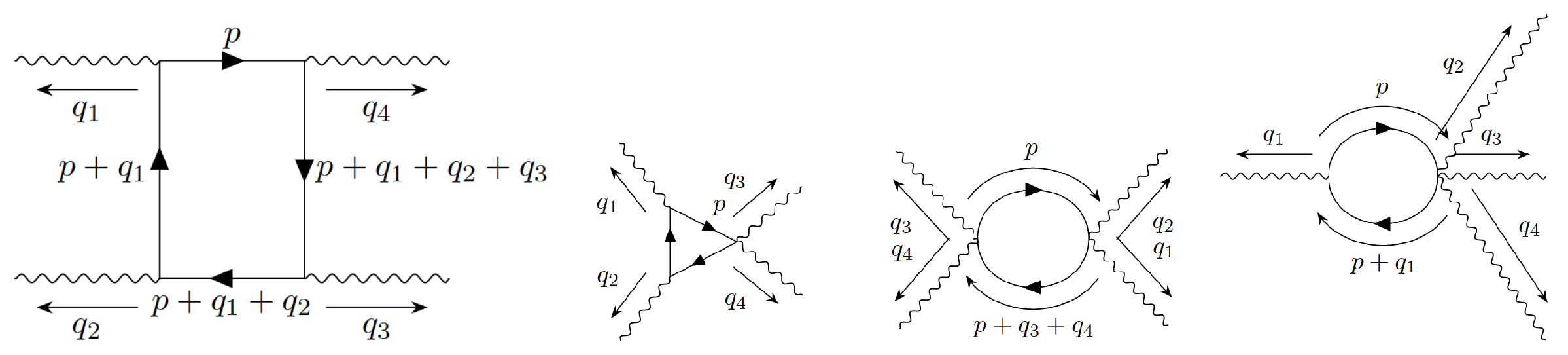
7. Photon–Photon Scattering in VSR QED

The Feynman rules are given in Appendix A. The graphs that contribute to photon–photon scattering in VSR QED are contained in Figure 5. To draw the graphs, we used [43].

It is easy to check that the infrared regularization implies that graphs (2, 3, 4) vanish, because the negative powers of $n·p$ are too large to be canceled by positive powers generated by the trace.

Define $V_{\mu }(p^{\prime },p)=\left({\gamma }_{\mu }+{\displaystyle \frac{1}{2}}{m}^2{\displaystyle \frac{\cancel{n}}{n·pn·p^{\prime }}}{n}_{\mu }\right)$, $S_F(p)=i{\displaystyle \frac{\cancel{p}+M-\frac{m^2}{2}\frac{\cancel{n}}{n·p}}{p^2-M_e^2+i\epsilon }}$

We verify this using graph (2).

$$\begin{array}{c}\hfill C_{{\mu }_1{\mu }_2{\mu }_3{\mu }_4}=-{(-i{e}^2)}^3{\displaystyle \frac{1}{2}}{n}_{{\mu }_3}{n}_{{\mu }_4}{m}^2\\ \hfill \int dpTr\left\{S_F(p)V_{{\mu }_1}(p+q_1,p)S_F(p+q_1)V_{{\mu }_2}(p+q_1+q_2,p+q_1)S_F(p+q_1+q_2)\cancel{n}\right\}\\ \hfill {\displaystyle \frac{1}{n·(p+q_1+q_2)}}{\displaystyle \frac{1}{n·p}}\left({\displaystyle \frac{1}{n·(q_3+p)}}+{\displaystyle \frac{1}{n·(q_4+p)}}\right)& \end{array}$$

The $Sim(2)$ symmetry implies the same number of $n_{\mu }$ in the numerator as in the denominator. But due to the new VSR vertex, two $n_{\mu }$s are outside the integral. In the denominator, we have three $n·p$-type factors, so the trace will produce at most one $n·p$ factor. The integral vanishes.

The same reasoning shows that graphs (3,4) vanish.

Moreover, graph (1) gives the standard QED result with electron mass given by $M_e=\sqrt{M^2+m^2}$, as required by unitarity. Thus:

$$\begin{array}{c}-{(-ie)}^4\int {\displaystyle \frac{d^{n}p}{{(2\pi )}^n}}Tr[V_{{\mu }_1}(p+q_1,p)S_F(p+q_1)V_{{\mu }_2}(p+q_1+q_2,p+q_1)S_F(p+q_1+q_2)\hfill \\ V_{{\mu }_3}(p+q_1+q_2+q_3,p+q_1+q_2)S_F(p+q_1+q_2+q_3)V_{{\mu }_4}(p,p+q_1+q_2+q_3)S_F(p)]=\\ -{(-ie)}^4\int {\displaystyle \frac{d^{n}p}{{(2\pi )}^n}}Tr[{\gamma }_{{\mu }_1}{S}_F^{\prime }(p+q_1){\gamma }_{{\mu }_2}{S}_F^{\prime }(p+q_1+q_2)\\ \hfill {\gamma }_{{\mu }_3}{S}_F^{\prime }(p+q_1+q_2+q_3){\gamma }_{{\mu }_4}{S}_F^{\prime }(p)]\end{array}$$

(38)

with $S_F^{\prime }(p)={\displaystyle \frac{i\left(\cancel{p}+M_e\right)}{p^2-M_e^2+i\epsilon }}$

Through the regularization procedure, we are using dimensional regularization. Then, the amplitude for photon–photon scattering is gauge-invariant [44].

We like to calculate the scattering cross section for this process.

7.1. Photon–Photon Scattering for $q_i^2\ll M_e^2$

The exact result for the amplitude is complicated [45].

Because the mass of the photon is very small, we will not have any difference from QED, except in the $q_i\to 0$ limit $q_i^2\ll M_e^2$. But in this zone, the amplitude goes to the Euler–Heisenberg Lagrangian, which is much simpler to write.

Keeping up to $o(F_{\mu \nu }^4)$, which describes photon–photon scattering, we obtain [46]:

$$\begin{array}{ccc}\hfill \mathcal{L}=-\mathcal{F}+{\displaystyle \frac{{\alpha }^2}{360}}{\displaystyle \frac{1}{M_e^4}}(4{(F_{\mu \nu }{F}^{\mu \nu })}^2+7{(F_{\mu \nu }{\tilde{F}}^{\mu \nu })}^2)& & \end{array}$$

(39)

where $\mathcal{F}={\displaystyle \frac{1}{4}}{F}_{\mu \nu }{F}^{\mu \nu }$, ${\tilde{F}}_{\mu \nu }={\displaystyle \frac{1}{2}}{\epsilon }_{\mu \nu \alpha \beta }{F}^{\alpha \beta }$; $\alpha$ is the fine structure constant.

From Equation (39), it is very simple to obtain the photon–photon scattering amplitude for $q_i^2\ll M_e^2$ [46]. It is:

$$\begin{array}{c}\hfill M=-{\displaystyle \frac{i{\alpha }^2}{45M_e^2}}{\displaystyle \frac{1}{12}}\\ \hfill (5(tr{f}_1{f}_{2}tr{f}_3{f}_4+tr{f}_1{f}_{3}tr{f}_2{f}_4+tr{f}_1{f}_{4}tr{f}_2{f}_3)\\ \hfill -7tr(f_1{f}_2{f}_3{f}_4+f_2{f}_1{f}_3{f}_4+f_3{f}_1{f}_2{f}_4+\\ \hfill f_2{f}_3{f}_1{f}_4+f_3{f}_2{f}_1{f}_4+f_1{f}_3{f}_2{f}_4))\end{array}$$

(40)

with $f_{i\rho \sigma }=i(q_{i\rho }{ϵ}_{i\sigma }-q_{i\sigma }{ϵ}_{i\rho })$

7.2. VSR Cross Section with Unpolarized Photons

The amplitude is formally equal to the QED result. The VSR characteristic is hidden in the vectors ${ϵ}_{i\sigma }$. Moreover, we have $q_{i\mu }{q}_i^{\mu }=m_{\gamma }^2$. The $Sim(2)$ symmetry allows us to write $n_{\mu }=(1,\widehat{n})$, $\widehat{n}.\widehat{n}=1$. For light-by-light scattering, we take $q_1=k_1,q_2=k_2,q_3=-k_3,q_4=-k_4$.

The sum over polarizations in VSR is given by [47]:

$$\begin{array}{cc}\hfill \sum _{\lambda }{ϵ}_{\mu }^{\lambda }(k){ϵ}_{\nu }^{\lambda *}(k)=-g_{\mu \nu }-{\displaystyle \frac{m_{\gamma }^2}{{(n·k)}^2}}{n}_{\mu }{n}_{\nu }+{\displaystyle \frac{1}{n·k}}(k_{\mu }{n}_{\nu }+k_{\nu }{n}_{\mu })& \end{array}$$

(41)

but, contracted with gauge-invariant terms $J^{\mu }$ that satisfy $k_{\mu }{J}^{\mu }=0$, it reduces to:

$$\begin{array}{cc}\hfill \sum _{\lambda }{ϵ}_{\mu }^{\lambda }(k){ϵ}_{\nu }^{\lambda *}(k)=-g_{\mu \nu }-{\displaystyle \frac{m_{\gamma }^2}{{(n·k)}^2}}{n}_{\mu }{n}_{\nu }& \end{array}$$

(42)

The unpolarized differential cross section is given by [46]:

$$\begin{array}{c}\hfill {\displaystyle \frac{d\sigma }{d\Omega }}={\displaystyle \frac{1}{{(2\pi )}^2}}{\displaystyle \frac{1}{2{\omega }^2}}{\displaystyle \frac{{\alpha }^4}{{(90)}^2{M}_e^8}}P\end{array}$$

(43)

P is written in Appendix G.

The total cross section is:

$$\begin{array}{cc}\hfill \sigma ={\displaystyle \frac{1}{{(2\pi )}^2}}{\displaystyle \frac{1}{2{\omega }^2}}{\displaystyle \frac{{\alpha }^4}{{(90)}^2{M}_e^8}}\int d\Omega P& \end{array}$$

To compute the total cross section $\sigma$, we work in the CM system. Most of the calculations have used FORM [34]. Then:

$$\begin{array}{ccc}\hfill k_1=(\omega ,\overrightarrow{k}),& & k_2=(\omega ,-\overrightarrow{k}),\hfill \\ \hfill k_3=(\omega ,{\overrightarrow{k}}^{\prime }),& & k_2=(\omega ,-{\overrightarrow{k}}^{\prime })\hfill \end{array}$$

To integrate over the solid angle, we choose polar coordinates for ${\overrightarrow{k}}^{\prime }$ with the z-axis in the direction of $\widehat{n}$. Keeping up to $o\left({\displaystyle \frac{m_{\gamma }^2}{{\omega }^2}}log\left({\displaystyle \frac{m_{\gamma }^2}{{\omega }^2}}\right)\right)$ and including the factor ${\displaystyle \frac{1}{2}}$ due to Bose statistics, we obtain:

$$\sigma ={\displaystyle \frac{973}{10125\pi }}{\displaystyle \frac{{\alpha }^4}{M_e^8}}{\omega }^6\left(1-{\displaystyle \frac{5}{56}}{\displaystyle \frac{m_{\gamma }^2}{{\omega }^2}}log\left({\displaystyle \frac{4{\omega }^2}{m_{\gamma }^2}}\right){(3+{cos}^2\alpha )}^2\right)$$

(44)

where $\overrightarrow{k}.\widehat{n}=kcos\alpha$. The result holds for $m_{\gamma }<\omega <M_e$.

The anisotropy of the leading correction shows the loss of rotational symmetry of VSR.

From the Particle Data Group [35]:

$$m_{\gamma }<3\times {10}^{-27}eV/c^2$$

(45)

For extremely low-frequency radio waves (ELF), $\omega \sim {10}^{-14}$ eV, corresponding to a wavelength $\lambda \sim {10}^8$ m, so the anisotropic term is very small and no conflict with present experimental data appears.

To detect the anisotropy, we have to look at cosmological scales. In fact, we expect that our result will produce tiny but measurable anisotropies in the Cosmic Microwave Background Radiation (CMB).

CMB anomalies have been pointed out since 20 years ago [48] and strong evidence of a dipole cosmic anisotropy has been accumulating [49].

In Ref. [22], we already speculated about the cosmic origin of the privileged direction in VSR, given by $\overrightarrow{n}$.

It is enticing to think that the physical cause of the small neutrino masses and tiny photon and graviton masses is due to a primordial dipole anisotropy of the Universe.

7.3. $2N$ Legs and Euler–Heisenberg Lagrangian

The same reasoning introduced at the beginning of Section 7 applies to 6, 8…$2N$ photon graphs.

We reach the following conclusions:

(1) Additional VSR graphs, obtained by the insertion of 2, 3, …$2N-1$ vertices, vanish in the $Sim(2)$ limit. In fact, the $Sim(2)$ symmetry implies the same number of $n_{\mu }$ in the numerator as in the denominator. But insertions of the new VSR vertices imply that $n_{\mu }$’s are outside the integral. Then, the number of $n·p$-type factors that are integrated over is negative. Therefore, the integral vanishes in the ${\overline{n}}_{\mu }=0$ limit.

(2) The remaining graphs corresponding to standard QED graphs reduce to the standard QED result with $M_e^2=M^2+m^2$ as required by unitarity.

Therefore, the ${\overline{n}}_{\mu }\to 0$ limit of the Euler–Heisenberg Lagrangian in VSR coincides with the E-H lagrangian in QED with $M_e^2=M^2+m^2$.

To obtain conclusion (2), use the $\cancel{n}$ to the right prescription and replace $m^2=M_e^2-M^2$. By explicit computation for $N=1,\dots ,4$, we found that M appears to be the first power alone. The coefficient of M is made of functions of $M_e^2$ multiplied by an odd number of Dirac’s matrices. So, their trace vanishes. This seems to hold for all N.

8. VSR Schwinger Model

A word of caution. In this section, we work in a 1 + 1 space-time, so the Lorentz group is a single-parameter group. As we discussed in [26], the two-dimensional Lorentz group acts as a scale transformation on the null vector $n_{\mu }=(1,1)$. So, we can introduce VSR-like mass terms for the fermions. When we refer to $Sim(2)$ symmetry or regulator in two dimensions, we mean the scale transformation mentioned above.

For a previous discussion of this model, please see Ref. [26].

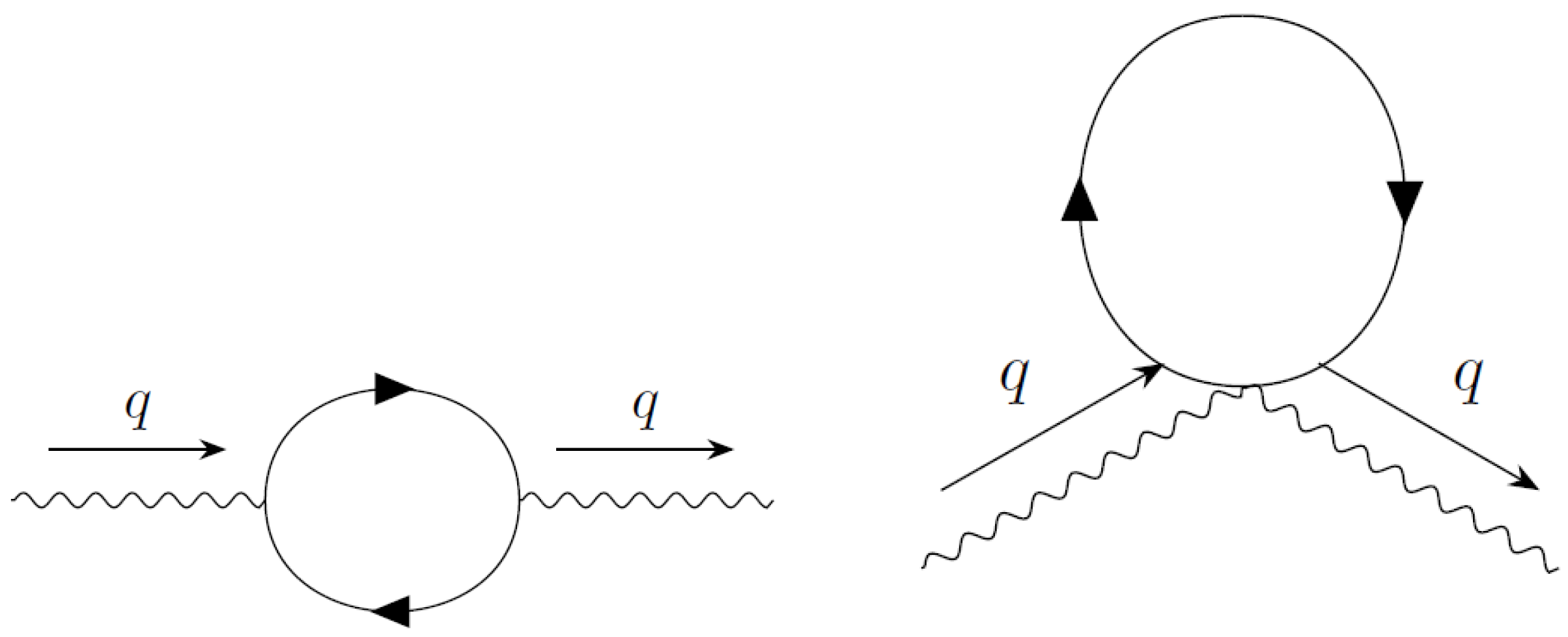
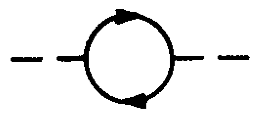
8.1. Photon Self Energy

Let us compute the photon self-energy. It is given by the two graphs of Figure 6:

$$\begin{array}{ccc}\hfill i{\Pi }_{1\mu \nu }=-e^2\int dpTr[({\gamma }_{\mu }+{\displaystyle \frac{n_{\mu }\cancel{n}{m}^2}{2n·(p+q)n·p}}){\displaystyle \frac{\left(\cancel{p}+M-\frac{m^2\cancel{n}}{2n·p}\right)}{p^2-M_e^2+i\epsilon }}& & \\ \hfill ({\gamma }_{\nu }+{\displaystyle \frac{n_{\nu }\cancel{n}{m}^2}{2n·(p+q)n·p}}){\displaystyle \frac{\left(\cancel{p}+\cancel{q}+M-\frac{m^2\cancel{n}}{2n·(p+q)}\right)}{{(p+q)}^2-M_e^2+i\epsilon }}]\end{array}$$

(46)

$$\begin{array}{cc}\hfill i{\Pi }_{2\mu \nu }=-e^2{n}_{\mu }{n}_{\nu }\int dp{\displaystyle \frac{1}{n·pn·(p+q)n·(p-q)}}Tr(\cancel{n}{m}^2{\displaystyle \frac{\left(\cancel{p}+M-\frac{m^2\cancel{n}}{2n·p}\right)}{p^2-M_e^2+i\epsilon }})& \end{array}$$

(47)

We use the ${\overline{n}}_{\mu }\to 0$ limit to evaluate the diagrams.

The second graph vanishes because there are three $n·p$s in the denominator and at most one $n·p$ in the numerator of the integrand. So, the ${\overline{n}}_{\mu }\to 0$ limit is zero. The counting of $n·p$ is determined by $Sim(2)$ symmetry. The second graph has 2 $n_{\mu }$ outside the integral, so there must be two $n·p$s in the denominator ($n·q$ is not factored outside the integral). The first graph gives:

$$\begin{array}{cc}\hfill i{\Pi }_{1\mu \nu }=4e^2\int {\displaystyle \frac{d^{d}p}{{(2\pi )}^d}}{\displaystyle \frac{-2p_{\mu }{p}_{\nu }-p_{\mu }{q}_{\nu }-p_{\nu }{q}_{\mu }-{\eta }_{\mu \nu }(M_e^2-p^2-p·q)}{(p^2-M_e^2+i\epsilon )({(p+q)}^2-M_e^2+i\epsilon )}}& \end{array}$$

(48)

Observe that some terms proportional to $m^2$ remain. They are produced by terms created by the trace of the form $m^{2}n·p,m^{2}n·(p+q)$. These terms balance the ${\displaystyle \frac{1}{n·p}},{\displaystyle \frac{1}{n·(p+q)}}$, so that after computing the $Sim(2)$ limit, they stay. These are precisely the factors we need to write the final result entirely in terms of the physical electron mass, $M_e^2=M^2+m^2$, which is expected from unitarity. This is the QED result, with the electron mass $M_e=\sqrt{M^2+m^2}$.

Using dimensional regularization, we obtain:

$$i{\Pi }_{1\mu \nu }=-2e^{2}i{\displaystyle \frac{tr(1)}{{(4\pi )}^{d/2}}}\Gamma \left(2-{\displaystyle \frac{d}{2}}\right){\int }_0^1{\displaystyle \frac{dx}{{(-q^{2}x(1-x)+M_e^2)}^{2-\frac{d}{2}}}}x(1-x)(q^2{\eta }_{\mu \nu }-q_{\mu }{q}_{\nu })$$

(49)

Put:

$$tr(1)=2,d=2$$

$$\begin{array}{cc}\hfill i{\Pi }_{\mu \nu }=-{\displaystyle \frac{e^2}{\pi }}i(q^2{\eta }_{\mu \nu }-q_{\mu }{q}_{\nu }){\int }_0^1{\displaystyle \frac{dx}{(-q^{2}x(1-x)+M_e^2)}}x(1-x)& \end{array}$$

If the fermion has a VSR mass $m\ne 0$, $M=0$, the photon stays massless. Only when $m=M=0$ does the photon obtains a mass $m_{\gamma }^2={\displaystyle \frac{e^2}{\pi }}$.

Using Equation (19.15) of [50], we obtain the vector current in the presence of an external electromagnetic field $A_{\mu }$:

$$\begin{array}{cc}\hfill <j^{\mu }(q)>=\int d^{2}x<j^{\mu }(x)>e^{iq.x}={\displaystyle \frac{i}{e}}(i{\Pi }^{\mu \nu }(q)A_{\nu }(q))& \end{array}$$

That is:

$$<j^{\mu }(q)>={\displaystyle \frac{e}{\pi }}(q^2{\eta }^{\mu \nu }-q^{\mu }{q}^{\nu })A_{\nu }(q){\int }_0^1{\displaystyle \frac{dx}{(-q^{2}x(1-x)+M_e^2)}}x(1-x)$$

(50)

It satisfies the conservation law $q_{\mu }<j^{\mu }(q)>=0$.

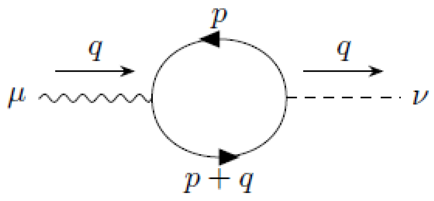
8.2. Two-Dimensional Axial Anomaly

In this case, we have to compute the expectation value of the axial vector current in a background field $A_{\nu }$. We follow the convention of [50], ${ϵ}^{01}=+1$.

$$<j^{5\nu }(q)>=\int d^{2}x<j^{5\nu }(x)>e^{iqx}={(-ie)}^{-1}i{\Pi }^{5\mu \nu }(q)A_{\mu }$$

(51)

The two-dimensional axial vector current in VSR electrodynamics is given by the two graphs (Figure 7 and Figure 8):

$$\begin{array}{c}\hfill i{\Pi }^{15\mu \nu }=-{(-ie)}^2\int dpTr\{\left[{\gamma }^{\mu }+{\displaystyle \frac{1}{2}}{n}^{\mu }\left(\cancel{n}\right)m^2{(n·(p+q))}^{-1}{(n·p)}^{-1}\right]\\ \hfill {\displaystyle \frac{i\left(\cancel{p}+M-\frac{m^2}{2}\frac{\cancel{n}}{n·p}\right)}{p^2-M^2-m^2+i\epsilon }}\left[{\gamma }^{\nu }+{\displaystyle \frac{1}{2}}{n}^{\nu }\left(\cancel{n}\right)m^2{(n·(p+q))}^{-1}{(n·p)}^{-1}\right]{\gamma }^5{\displaystyle \frac{i\left(\left(\cancel{p}+\cancel{q}\right)+M-\frac{m^2}{2}\frac{\cancel{n}}{n·(p+q)}\right)}{{(p+q)}^2-M_e^2+i\epsilon }}\}\end{array}$$

(52)

$$\begin{array}{c}\hfill i{\Pi }^{25\mu \nu }=(-1){(ie)}^2{n}^{\mu }{n}^{\nu }i\int dp{(n·p)}^{-1}{(n·p)}^{-1}[{(n·(q+p))}^{-1}+{(n·(-q+p))}^{-1}]\\ \hfill Tr\{{\displaystyle \frac{1}{2}}\cancel{n}{m}^2{\displaystyle \frac{i\left(\cancel{p}+M-\frac{m^2}{2}\frac{\cancel{n}}{n·p}\right)}{p^2-M_e^2+i\epsilon }}{\gamma }^5\}& & \end{array}$$

(53)

Notice that this is a new vertex with one photon line and one axial vector line (current insertion). Please see Figure A2 in Appendix A.

This graph vanishes in the $Sim(2)$ limit. There are three $n·p$s in the denominator and at most one $n·p$ in the numerator of the integrand, where $p_{\mu }$ is the integration variable. According to the rules of Section 3, the integral vanishes when ${\overline{n}}_{\mu }\to 0$. Now, we compute the $Sim(2)$ limit of ${\Pi }^{15\mu \nu }$.

We have to study the behavior of the ${\overline{n}}_{\mu }\to 0$ limit in the presence of ${\gamma }_5$. It is straightforward to do so. We must use, from the beginning the standard definition of ${\gamma }_5$ in the corresponding dimension, ${\gamma }_5=i{\gamma }_0{\gamma }_1$ in two dimensions, and ${\gamma }_5=i{\gamma }_0{\gamma }_1{\gamma }_2{\gamma }_3$ in four dimensions. Then, we displace all $\cancel{n}$ to the right, collect all $n·(p+R)$ produced by this motion, and use them to cancel as many $n·(p+R)$ in the denominator as possible. At the end, all remaining ${(n·(p+R))}^{-a},a>0$ are substituted by zero. Here, $R_{\mu }$ means any vector different from $p_{\mu }$ (the integration variable), with the zero vector included.

We obtain the standard QED answer with the physical fermion mass: $M_e^2=M^2+m^2.$

$$i{\Pi }_{1\mu \nu }^5=-e^2\int dp{\displaystyle \frac{Tr\left\{{\gamma }_{\mu }\cancel{p}{\gamma }_{\nu }{\gamma }_5\cancel{p}+{\gamma }_{\mu }\cancel{p}{\gamma }_{\nu }{\gamma }_5\cancel{q}+M_e^2{\gamma }_{\mu }{\gamma }_{\nu }{\gamma }_5\right\}}{(p^2-M_e^2+i\epsilon )({(p+q)}^2-M_e^2+i\epsilon )}}$$

(54)

Using the two-dimensional identity:

$${\gamma }^{\mu }{\gamma }_5=-{\epsilon }^{\mu \alpha }{\gamma }_{\alpha }$$

We obtain $i{\Pi }_{1\mu \nu }^5=-{ϵ}_{\nu \alpha }i{\Pi }_{\mu }^{\alpha }$, which implies

$$<j^{\mu 5}(q)>=-{\epsilon }^{\mu \nu }<j_{\nu }(q)>$$

(55)

From Equations (50) and (55), the divergence of the axial current is:

$$\begin{array}{cc}\hfill <j^{\mu 5}(q)>q_{\mu }=-{\displaystyle \frac{e}{\pi }}{q}^2{\epsilon }^{\mu \nu }{q}_{\mu }{A}_{\nu }(q){\int }_0^1{\displaystyle \frac{dx}{(-q^{2}x(1-x)+M_e^2)}}x(1-x)& \end{array}$$

(56)

Equation (56) agrees with the calculation of the divergence of the axial current obtained in [26] with $M=0$. In [27], we computed the same quantity and obtained the standard anomaly, i.e., Equation (56) with $m=0,M=0$. We will see below that the different results are a matter of interpretation. In fact, we can see that a $Sim(2)$ regulator will break the chiral symmetry by generating a standard fermion mass. So, we obtain:

$$\begin{array}{cc}\hfill {\partial }_{\mu }{j}^{\mu 5}(x)={\displaystyle \frac{e}{2\pi }}{\epsilon }^{\mu \nu }{F}_{\mu \nu }+2M_e\overline{\psi }{\gamma }_5\psi & \end{array}$$

(57)

In fact, define $K_{\mu }$ by:

$$\int d^{2}x<\overline{\psi }(x){\gamma }_5\psi (x)>e^{iqx}=K^{\mu }(q)A_{\mu }(q)$$

(58)

We obtain:

$$\begin{array}{ccc}\hfill K^{\mu }=-(-ie)\int dp{\displaystyle \frac{Tr\left\{{\gamma }^{\mu }i\left(\cancel{p}+M_e\right){\gamma }_{5}i\left(\cancel{p}+\cancel{q}+M_e\right)\right\}}{(p^2-M_e^2+i\epsilon )({(p+q)}^2-M_e^2+i\epsilon )}}=& & \\ \hfill {\displaystyle \frac{M_e}{2\pi }}e{\epsilon }^{\mu \alpha }{q}_{\alpha }\int dx{\displaystyle \frac{1}{M_e^2-q^{2}x(1-x)-i\epsilon }}& \end{array}$$

(59)

Notice that $K^{\mu }{q}_{\mu }=0$, as implied by gauge invariance.

Then:

$$\begin{array}{cc}\hfill <j^{\mu 5}(q)>q_{\mu }-2M_e{K}^{\mu }{A}_{\mu }={\displaystyle \frac{e}{\pi }}{\epsilon }^{\mu \nu }{q}_{\mu }{A}_{\nu }(q)& \end{array}$$

(60)

The divergence of the chiral current obtains two contributions; one is due to a non-zero mass: $2M_e\overline{\psi }{\gamma }_5\psi$. The other is the anomaly, which is present even for a massless fermion model with $M=m=0$. The main difference is that the contribution of the mass is finite and unambiguous. The anomaly term requires an ultraviolet (UV) regulator that breaks the chiral symmetry. In a model with a VSR mass, the infrared regularization introduces a mass-like term that contributes to the divergence of the chiral current as well as the standard anomaly.

This observation permits us to understand the results of the anomaly obtained in [26,27].

The result of [26] corresponds to considering the non-zero divergence of the chiral current as the anomaly. Instead, in [27] we computed the standard anomaly, which is present even for zero fermion mass, as a result of the UV regulator.

8.3. Anomaly Calculation in Dimensional Regularization

In this subsection, we will directly compute the expectation value of the chiral current using dimensional regularization instead of using Equation (55). To treat ${\gamma }^5$, we follow the prescription of [51]. That is, in any number of dimensions

$$\begin{array}{ccc}\hfill {\gamma }^5& =i{\gamma }^0{\gamma }^1,& \end{array}$$

(61)

$$\begin{array}{cc}\hfill \{{\gamma }^5,{\gamma }^{\mu }\}=0.\mu =0,1;& [{\gamma }^5,{\gamma }^{\mu }]=0,\mu =2,3,\dots .,d\end{array}$$

(62)

$q_{\mu },n^{\mu }$ are two-dimensional vectors. $p_{\mu }$ is d-dimensional.

We found Equation (54) in the previous subsection:

$$\begin{array}{c}\hfill i{\Pi }_{1\mu \nu }^5=-e^2\int dp\\ \hfill {\displaystyle \frac{Tr\left\{{\gamma }_{\mu }\cancel{p}{\gamma }_{\nu }{\gamma }_5\cancel{p}+{\gamma }_{\mu }\cancel{p}{\gamma }_{\nu }{\gamma }_5\cancel{q}+M_e^2{\gamma }_{\mu }{\gamma }_{\nu }{\gamma }_5\right\}}{(p^2-M_e^2+i\epsilon )({(p+q)}^2-M_e^2+i\epsilon )}}\end{array}$$

Write $\cancel{p}={\cancel{p}}_1+{\cancel{p}}_2$ with $p_{1\mu },\mu =0,1$; $p_{2\mu },\mu =2,\dots ,d$. Then:

$$\begin{array}{c}\hfill i{\Pi }_{1\mu \nu }^5=-e^2{\int }_0^{1}dx\int dp\\ \hfill {\displaystyle \frac{Tr\left\{{\gamma }_{\mu }{\cancel{p}}_1{\gamma }_{\nu }{\gamma }_5{\cancel{p}}_1+{\gamma }_{\mu }{\cancel{p}}_2{\gamma }_{\nu }{\gamma }_5{\cancel{p}}_2+(x^2-x){\gamma }_{\mu }\cancel{q}{\gamma }_{\nu }{\gamma }_5\cancel{q}+M_e^2{\gamma }_{\mu }{\gamma }_{\nu }{\gamma }_5\right\}}{{(p^2-M_e^2+i\epsilon +q^{2}x(1-x))}^2}}\end{array}$$

Using dimensional regularization, the numerator can be replaced by:

$$\begin{array}{c}\hfill Tr\left({\gamma }_{\mu }{\cancel{p}}_1{\gamma }_{\nu }{\gamma }_5{\cancel{p}}_1\right)=-{{\epsilon }_{\nu }}^{\alpha }Tr\left({\gamma }_{\mu }{\cancel{p}}_1{\gamma }_{\alpha }{\cancel{p}}_1\right)\to -{{\epsilon }_{\nu }}^{\alpha }\left(4{\displaystyle \frac{1}{2}}{p}_1^2{\eta }_{\mu \alpha }-2p_1^2{\eta }_{\mu \alpha }\right)=0\end{array}$$

(63)

$$\begin{array}{cc}\hfill Tr\left({\gamma }_{\mu }{\cancel{p}}_2{\gamma }_{\nu }{\gamma }_5{\cancel{p}}_2\right)=-p_2^{2}Tr({\gamma }_{\mu }{\gamma }_{\nu }{\gamma }_5)\to -p^2{\displaystyle \frac{d-2}{d}}Tr({\gamma }_{\mu }{\gamma }_{\nu }{\gamma }_5)& \end{array}$$

(64)

But,

$${\displaystyle \frac{d-2}{d}}\int dp{\displaystyle \frac{p^2}{{(p^2-M_e^2+i\epsilon +q^{2}x(1-x))}^2}}={\displaystyle \frac{i}{4\pi }}$$

Therefore:

$$i{\Pi }_{1\mu \nu }^5=-e^2{\displaystyle \frac{i}{\pi }}(q^2{\epsilon }_{\mu \nu }+q_{\mu }{\epsilon }_{\nu \alpha }{q}^{\alpha })\int dx{\displaystyle \frac{x(1-x)}{M_e^2-q^{2}x(1-x)}}$$

(65)

That is, the divergence of the axial current is

$$q_{\mu }<j^{\mu 5}>={\displaystyle \frac{i}{e}}i{\Pi }_1^{\mu \nu 5}{q}_{\nu }{A}_{\mu }=-{\displaystyle \frac{e}{2\pi }}{q}^2{\epsilon }^{\mu \nu }{F}_{\mu \nu }\int dx{\displaystyle \frac{x(1-x)}{M_e^2-q^{2}x(1-x)}}$$

which coincides with Equation (56).

In the massless case, we recover Equation (19.18) of [50]. If $M=0$, we have conservation of chiral symmetry at the classical level in VSR QED, but this symmetry is broken at the quantum level. We can consider the above expression as the anomaly as in [26] or interpret the anomaly as the one corresponding to the massless case [27] and the remaining, being finite and unambiguous, as the mass contribution to the divergence of the chiral current.

9. Four-Dimensional Axial Anomaly

We compute:

$$\int d^{4}x{e}^{-irx}<p,q\left|j^{\mu 5}(x)\right|0>={(2\pi )}^4\delta (-r+p+q){\epsilon }_{\nu }^{*}(q){\epsilon }_{\delta }^{*}(p)i{\Pi }^{\mu \nu \delta }$$

There are four topologically distinct graphs, plus permutations of the external legs, that add to the axial anomaly in four dimensions (Figure 9, Figure 10, Figure 11 and Figure 12). The Feynman rules are written in Appendix A, Figure A2. They are crucial to satisfying the formal Ward identity for the vector current (charge conservation) as well as the right computation of the axial anomaly [27].

$$\begin{array}{c}i{\Pi }^{15\mu \nu \delta }=-{(-ie)}^2\int dkTr\{\left[{\gamma }^{\mu }+{\displaystyle \frac{1}{2}}{\displaystyle \frac{n^{\mu }\cancel{n}{m}^2}{n·(k+q)n·(k-p)}}\right]{\gamma }^5\\ {\displaystyle \frac{i\left(\left(\cancel{k}+\cancel{q}\right)+M-\frac{m^2}{2}\frac{\cancel{n}}{n·(k+q)}\right)}{{(k+q)}^2-M^2-m^2+i\epsilon }}\\ \left[{\gamma }^{\nu }+{\displaystyle \frac{1}{2}}{\displaystyle \frac{n^{\nu }\cancel{n}{m}^2}{n·(k+q)n·k}}\right]{\displaystyle \frac{i\left(\cancel{k}+M-\frac{m^2}{2}\frac{\cancel{n}}{n·k}\right)}{k^2-M^2-m^2+i\epsilon }}\\ \left[{\gamma }^{\delta }+{\displaystyle \frac{1}{2}}{\displaystyle \frac{n^{\delta }\cancel{n}{m}^2}{n·(k-p)n·k}}\right]{\displaystyle \frac{i\left(\cancel{k}-\cancel{p}+M-\frac{m^2}{2}\frac{\cancel{n}}{n·(k-p)}\right)}{{(k-p)}^2-M^2-m^2+i\epsilon }}\}+(p,\delta )\to (q,\nu )\end{array}$$

(66)

$$\begin{array}{c}\hfill i{\Pi }^{25\mu \nu \delta }=(-1){(ie)}^2{n}^{\delta }{n}^{\nu }i\int dk{\displaystyle \frac{1}{n·kn·(k-p-q)}}[{\displaystyle \frac{1}{n·(k-q)}}+{\displaystyle \frac{1}{n·(k-p)}}]\\ \hfill Tr\{{\displaystyle \frac{1}{2}}\cancel{n}{m}^2{\displaystyle \frac{i\left(\cancel{k}-\cancel{p}-\cancel{q}+M-\frac{m^2}{2}\frac{\cancel{n}}{n·(k-p-q)}\right)}{{(k-p-q)}^2-M_e^2+i\epsilon }}\left[{\gamma }^{\mu }+{\displaystyle \frac{1}{2}}{\displaystyle \frac{n^{\mu }\cancel{n}{m}^2}{n·kn·(k-p-q)}}\right]{\gamma }^5& & \\ \hfill {\displaystyle \frac{i\left(\cancel{k}+M-\frac{m^2}{2}\frac{\cancel{n}}{n·k}\right)}{k^2-M_e^2+i\epsilon }}\}\end{array}$$

(67)

$$\begin{array}{c}i{\Pi }^{35\mu \nu \delta }=(-1){(ie)}^2{n}^{\delta }{n}^{\mu }i\int dk{\displaystyle \frac{1}{n·kn·(k-q)}}[{\displaystyle \frac{1}{n·(k-q-p)}}+{\displaystyle \frac{1}{n·(k+p)}}]\\ Tr\left\{{\displaystyle \frac{1}{2}}\cancel{n}{m}^2{\gamma }^5{\displaystyle \frac{i\left(\cancel{k}+M-\frac{m^2}{2}\frac{\cancel{n}}{n·k}\right)}{k^2-M^2-m^2+i\epsilon }}\left[{\gamma }^{\nu }+{\displaystyle \frac{1}{2}}{\displaystyle \frac{\cancel{n}{n}^{\nu }{m}^2}{n·kn·(k-q)}}\right]{\displaystyle \frac{i\left(\cancel{k}-\cancel{q}+M-\frac{m^2}{2}\frac{\cancel{n}}{n·(k-q)}\right)}{{(k-q)}^2-M^2-m^2+i\epsilon }}\right\}\\ +(p,\delta )\to (q,\nu )\end{array}$$

(68)

$$\begin{array}{c}i{\Pi }^{45\mu \nu \delta }=i{e}^2{n}^{\nu }{n}^{\mu }{n}^{\delta }i\int dk{\displaystyle \frac{1}{{(n·k)}^2}}[{\displaystyle \frac{1}{n·(k+p+q)}}{\displaystyle \frac{1}{n·(k+p)}}+{\displaystyle \frac{1}{n·(k+p+q)}}{\displaystyle \frac{1}{n·(k+q)}}+\\ {\displaystyle \frac{1}{n·(k-p)}}{\displaystyle \frac{1}{n·(k-p-q)}}+{\displaystyle \frac{1}{n·(k-q)}}{\displaystyle \frac{1}{n·(k+p)}}+{\displaystyle \frac{1}{n·(k-p)}}{\displaystyle \frac{1}{n·(k+q)}}+\\ {\displaystyle \frac{1}{n·(k-q)}}{\displaystyle \frac{1}{n·(k-p-q)}}]Tr\left\{{\displaystyle \frac{1}{2}}\cancel{n}{m}^2{\gamma }^{5}i{\displaystyle \frac{i\left(\cancel{k}+M-\frac{m^2}{2}\frac{\cancel{n}}{n·k}\right)}{k^2-M^2-m^2+i\epsilon }}\right\}\end{array}$$

(69)

But the ${\overline{n}}_{\mu }\to 0$ limit easily shows that the graphs with insertions of non-standard QED vertices, Figure 10, Figure 11 and Figure 12, vanish. In fact, Figure 10 contains two $n_{\mu }$s outside the integral. $Sim(2)$ symmetry means that there are two ${\displaystyle \frac{1}{n·(k+R)}}$s inside the integral. That is, the integral is proportional to ${\overline{n}}_{\alpha }{\overline{n}}_{\beta }\to 0$. The same discussion implies that graphs (11,12) vanish.

The standard graphs, Figure 9, stay.

We have to investigate the ${\overline{n}}_{\mu }\to 0$ limit in the presence of ${\gamma }_5$. As we carried out in two dimensions, we must use, from the beginning the standard definition of ${\gamma }_5$ in the corresponding dimension, ${\gamma }_5=i{\gamma }_0{\gamma }_1{\gamma }_2{\gamma }_3$ in four dimensions. We displace all $\cancel{n}$ to the right, collect all $n·(p+R)$ produced by this motion, and use them to cancel as many $n·(p+R)$ in the denominator as possible. At the end, all remaining ${(n·(p+R))}^{-a},a>0$ are replaced by zero. Here, $R_{\mu }$ means any vector different from $p_{\mu }$ (the integration variable), the zero vector included.

The result agrees with standard QED with a mass $M_e$:

$$\begin{array}{cc}\hfill i{\Pi }^{15\mu \nu \delta }=e^2\int dkTr\left\{{\gamma }^{\mu }{\gamma }_{5}i{\displaystyle \frac{\cancel{k}+\cancel{q}+M_e}{{(k+q)}^2-M_e^2+i\epsilon }}{\gamma }^{\nu }i{\displaystyle \frac{\cancel{k}+M_e}{k^2-M_e^2+i\epsilon }}{\gamma }^{\delta }i{\displaystyle \frac{\cancel{k}-\cancel{p}+M_e}{{(k-p)}^2-M_e^2+i\epsilon }}\right\}& \end{array}$$

(70)

This is a great simplification.

Therefore, the divergence of the axial vector current has two terms: the same anomaly as in standard QED when $M=m=0$, plus a mass term if either $M\ne 0$ or $m\ne 0$. If $M=0$ and $m\ne 0$, the axial vector current is conserved classically but is broken at the quantum level by a mass term.

10. Gross–Neveu Model in VSR

Please see the word of caution at the beginning of Section 8.

We follow [52]. We add a VSR mass m to the fermion.

$$\begin{array}{cc}\hfill \mathcal{L}={\overline{\psi }}^a\left(i\left(\cancel{\partial }+{\displaystyle \frac{1}{2}}\cancel{n}{m}^2{(n·\partial )}^{-1}\right)\right){\psi }^a+{\displaystyle \frac{g_0}{2N}}{({\overline{\psi }}^a{\psi }^a)}^2& \end{array}$$

(71)

The Lagrangian is invariant under the discrete chiral symmetry:

$${\psi }^a\to {\gamma }_5{\psi }^a,{\overline{\psi }}^a\to -{\overline{\psi }}^a{\gamma }_5$$

The large N limit can be obtained by the introduction of a boson field $\sigma$.

$$\begin{array}{ccc}\hfill \mathcal{L}={\overline{\psi }}^a\left(i\left(\cancel{\partial }+{\displaystyle \frac{1}{2}}\cancel{n}{m}^2{(n·\partial )}^{-1}\right)\right){\psi }^a+{\displaystyle \frac{g_0}{2N}}{({\overline{\psi }}^a{\psi }^a)}^2-{\displaystyle \frac{N}{2g_0}}{\left(\sigma -{\displaystyle \frac{g_0}{N}}{\overline{\psi }}^a{\psi }^a\right)}^2\to & & \\ \hfill {\overline{\psi }}^a\left(i\left(\cancel{\partial }+{\displaystyle \frac{1}{2}}\cancel{n}{m}^2{(n·\partial )}^{-1}\right)\right){\psi }^a-{\displaystyle \frac{N}{2g_0}}{\sigma }^2+\sigma {\overline{\psi }}^a{\psi }^a& \end{array}$$

(72)

The generating functional is obtained by integrating over the fermion fields to obtain:

$$\begin{array}{cc}\hfill Z=\int d\sigma e^{i\int dx\left(-{\displaystyle \frac{N}{2g_0}}{\sigma }^2\right)+tr\left(log\left(i\left(\cancel{\partial }+{\displaystyle \frac{1}{2}}\cancel{n}{m}^2{(n·\partial )}^{-1}+\sigma (x)\right)\right)\right)}& \end{array}$$

(73)

To find the vacuum, we just need the effective potential $V_{eff}$. $\sigma$ is independent of $x^{\mu }$.

$$\begin{array}{cc}\hfill -i{V}_{eff}(\sigma )=-i{\displaystyle \frac{N}{2g_0}}{\sigma }^2+tr\left(log\left(i\left(\cancel{\partial }+{\displaystyle \frac{1}{2}}\cancel{n}{m}^2{(n·\partial )}^{-1}+\sigma \right)\right)\right)& \end{array}$$

(74)

Thus:

$$-i{V}_{eff}(\sigma )=-i{\displaystyle \frac{N}{2g_0}}{\sigma }^2-\sum _{n=1}{\displaystyle \frac{N}{2n}}Tr\int dp{\displaystyle \frac{{(p^2-m^2)}^n}{{(p^2-m^2+i\epsilon )}^{2n}}}{\sigma }^{2n}$$

(75)

We see that we do not have infrared divergences in the effective potential. We do need the infrared regulator of Section 3 if we want to compute the effective action. For instance, Figure 13 needs the infrared regulator for arbitrary external momentum.

We calculate the effective potential using dimensional regularization in the minimal subtraction scheme (MS). $\mu$ is the arbitrary scale introduced in dimensional regularization.

The model is renormalizable.

The renormalized coupling g in MS is: ${\displaystyle \frac{1}{g}}={\displaystyle \frac{1}{g_0}}-{\displaystyle \frac{1}{\pi \epsilon }},\epsilon =2-d$.

We obtain:

$${\displaystyle \frac{1}{N}}{V}_{eff}={\sigma }^2\left({\displaystyle \frac{1}{2g}}-{\displaystyle \frac{{\Gamma }^{\prime }(1)}{4\pi }}-{\displaystyle \frac{1}{4\pi }}\right)+{\displaystyle \frac{1}{4\pi }}{m}^{2}log\left({\displaystyle \frac{{\sigma }^2}{m^2}}+1\right)+{\displaystyle \frac{{\sigma }^2}{4\pi }}log\left({\displaystyle \frac{{\sigma }^2+m^2}{4\pi {\mu }^2}}\right)$$

(76)

To compare with [52] Equation (2.26), choose

$$\begin{array}{cc}\hfill log(4\pi {\mu }^2)=log(M^2)+2-{\Gamma }^{\prime }(1)& \end{array}$$

We obtain:

$${\displaystyle \frac{1}{N}}{V}_{eff}={\displaystyle \frac{{\sigma }^2}{2g}}+{\displaystyle \frac{1}{4\pi }}{m}^{2}log\left({\displaystyle \frac{{\sigma }^2}{m^2}}+1\right)+{\displaystyle \frac{{\sigma }^2}{4\pi }}\left(log\left({\displaystyle \frac{{\sigma }^2+m^2}{M^2}}\right)-3\right)$$

(77)

It goes to Coleman’s Equation (2.26) when $m\to 0$.

The ground state ${\sigma }_0$ is the absolute minimum of $V_{eff}$. It satisfies:

$${\displaystyle \frac{{\sigma }_0\left(log\left(\frac{{{\sigma }_0}^2+m^2}{M^2}\right)-3\right)}{2\pi }}+{\displaystyle \frac{{\sigma }_0}{2\pi \left(\frac{{\sigma }_0^2}{m^2}+1\right)}}+{\displaystyle \frac{{\sigma }_0^3}{2\pi ({\sigma }_0^2+m^2)}}+{\displaystyle \frac{{\sigma }_0}{g}}=0$$

(78)

i.e., ${\sigma }_0=0$ or

$${\sigma }_0^2=M^2{e}^{2-{\displaystyle \frac{2\pi }{g}}}-m^2$$

(79)

Notice that now we have the additional condition that $M^2{e}^{2-{\displaystyle \frac{2\pi }{g}}}-m^2\ge 0$. ${\sigma }_0^2+m^2$ is a physical quantity. Thus, it satisfies the homogeneous renormalization group equation:

$$\begin{array}{c}\hfill \left(M{\displaystyle \frac{\partial }{\partial M}}+\beta (g){\displaystyle \frac{\partial }{\partial g}}\right)({\sigma }_0^2+m^2)=0\end{array}$$

(80)

$$\begin{array}{c}\hfill \beta (g)=-{\displaystyle \frac{g^2}{\pi }}\end{array}$$

(81)

So, in the phase where $M^2{e}^{2-{\displaystyle \frac{2\pi }{g}}}-m^2\ge 0$, the model is asymptotically free. It is easy to verify that if $M^2{e}^{2-{\displaystyle \frac{2\pi }{g}}}-m^2\ge 0$, then ${\sigma }_0$ is a global minimum of $V_{eff}$.

The running coupling is:

$$g={\displaystyle \frac{g_0}{1+\frac{g_0}{\pi }log\left(\frac{M}{M_0}\right)}}$$

(82)

The model has two phases:

• $M^2{e}^{2-{\displaystyle \frac{2\pi }{g}}}-m^2\ge 0,{\sigma }_0\ne 0$. The discrete chiral symmetry is spontaneously broken.
• $M^2{e}^{2-{\displaystyle \frac{2\pi }{g}}}-m^2<0,{\sigma }_0=0$, The discrete chiral symmetry is preserved.

11. Conclusions

In this paper, we have reviewed the prescription introduced in [23] to obtain the $Sim(2)$ limit of VSR graphs, infrared regularized using the ML regularization. In ML, besides the $n_{\mu }$ null vector of VSR theories, a second null vector ${\overline{n}}_{\mu }$ is required. ML preserves naive power counting and gauge invariance but destroys the $Sim(2)$ symmetry.

To recover the $Sim(2)$ symmetry, we take the limit ${\overline{n}}_{\mu }\to 0$. For scalar integrals, this limit is well defined and straightforward.

In the presence of $\gamma$ matrices, we need to introduce a prescription. In this paper, we used the convention to move all $\cancel{n}$ to the right and then take ${\overline{n}}_{\mu }\to 0$. In Appendix E, we present the method of traces to compute ${\overline{n}}_{\mu }\to 0$. In VSR QED, both methods give the same answer.

${\overline{n}}_{\mu }\to 0$ chooses a subset of integrals defining the $Sim(2)$ regularized Feynman graphs. The Ward identities are satisfied among graphs belonging to this subset.

Using this prescription, we proceed to compute the single-loop renormalization of VSR QED with a gauge-invariant photon mass. We have shown that the photon self energy is transverse and that the Ward–Takahashi identity is satisfied for the $Sim(2)$-invariant graphs.

Then, we computed the three vertex on shell and checked that it is conserved; we extracted the form factors and computed the anomalous magnetic moment of the electron corrected by non-zero neutrino and photon mass.

Using the most recent data for the photon mass, we obtain a bound for the electron neutrino mass.

As a second application of the regulator, we computed the unpolarized differential cross section for photon–photon scattering in VSR QED with a gauge-invariant photon mass in terms of Lorentz scalar functions (Appendix G). We restricted our calculation to ${\overrightarrow{k}}_i^2<M_e^2$ because for higher values of the momenta, VSR QED coincides with QED. Using this result, we have obtained the leading contribution in the limit $m_{\gamma }\to 0$ to the total cross section $\sigma$ in the CM system. The leading contribution is anisotropic, exhibiting the loss of rotational invariance of VSR models. But the photon mass term is very small, so no conflict with available experimental data appears.

We expect that our result will produce tiny but measurable anisotropies in the Cosmic Microwave Background Radiation (CMB). The anisotropy is due to a preferred direction $\widehat{n}$.

We applied the infrared regulator to single-loop amplitudes with an arbitrary number of photon legs, reaching the ensuing conclusions:

(1) Additional VSR graphs, obtained by the insertion of 2, 3,…$2N-1$ vertices, vanish in the $Sim(2)$ limit.

(2) The remaining graphs corresponding to standard QED graphs reduce to the standard QED result with $M_e^2=M^2+m^2$ as required by unitarity.

Therefore, the ${\overline{n}}_{\mu }\to 0$ limit of the Euler–Heisenberg Lagrangian in VSR coincides with the E-H lagrangian in QED with $M_e^2=M^2+m^2$ as required by unitarity.

Lastly, we broaden the infrared regularization of [23] to accept terms with ${\gamma }_5$. We have verified that $Sim(2)$ and gauge symmetries are preserved.

In this context, we first consider the two-dimensional anomaly in the Schwinger model. We have explicitly checked that the result is gauge-invariant and produces the standard anomaly. In addition, by calculating the mass contribution to the divergence of the axial current, we were able to clarify the different results obtained in previous works [26,27]. In [26], we obtained the divergence of the axial current in the presence of a VSR fermion mass. We find the same answer in the present paper for $M=0$. In [27], we obtained the standard anomaly produced by the ultraviolet divergences. According to the analysis we have carried out now, the divergence of the axial current receives two contributions: the anomaly, which is present even for massless fermions, and the mass term. If we introduce a VSR fermion mass, the axial vector current is conserved at the classical level, but is violated at the quantum level by the anomaly due to ultraviolet divergences, and by a mass term. The mass term seems to be unavoidable if we want to preserve $Sim(2)$ symmetry at the quantum level.

As a second application of the infrared regulator, we computed the triangle anomaly in four-dimensional QED with a VSR fermion mass. Again, the regulator adds the VSR terms in such a way that the final answer is the same as the standard QED one with the physical mass for the fermion $M_e=\sqrt{M^2+m^2}$. It follows that we obtain the standard anomaly as in [27] plus a VSR mass contributions to the divergence of the axial current.

As a last example, we solved the Gross–Neveu (GN) model with a VSR fermion mass. We discovered that the VSR mass m allows the existence of two phases. In one of them, the chiral symmetry is broken as in the standard GN model; in the new phase, the chiral symmetry is unbroken.

The $Sim(2)$ regulator we reviewed in this paper is very simple and reduces all integrals to standard dimensionally regularized integrals. It is universal, i.e, it applies to all VSR graphs because the zero vector is an invariant vector for $Sim(2)$ too. It can be applied to all sorts of VSR theories, not just VSR QED. We are guaranteed to preserve the gauge invariance of the model.

Many applications are feasible: VSR extension of the Nambu–Jona–Lasinio model, considering the implications of VSR masses for fermions in supersymmetric and superstring models, and loop computations in the VSRSM including the three families of quarks and leptons, among others.

References

1. Langacker, P. The Standard Model and Beyond; CRC Press: Boca Raton, FL, USA; Taylor and Francis Group: Abingdon, UK, 2010. [Google Scholar]
2. Mohapatra, R. Unification and Supersymmetry: The Frontiers of Quark-Lepton Physics, 3rd ed.; Springer: New York, NY, USA, 2002. [Google Scholar]
3. Pierre Auger Collaboration. Observation of the Suppression of the Flux of Cosmic Rays above 4 × 10¹⁹eV. Phys. Rev. Lett. 2008, 101, 061101. [Google Scholar] [CrossRef] [PubMed]
4. Amelino-Camelia, G. Quantum-Spacetime Phenomenology. Living Rev. Relativ. 2013, 16, 5. [Google Scholar] [CrossRef] [PubMed]
5. Jacobson, T.; Liberati, S.; Mattingly, D. Astrophysical Bounds on Planck Suppressed Lorentz Violation. Lect. Notes Phys. 2005, 669, 101. [Google Scholar]
6. Myers, R.C.; Pospelov, M. Ultraviolet Modifications of Dispersion Relations in Effective Field Theory. Phys. Rev. Lett. 2003, 90, 211601. [Google Scholar] [CrossRef]
7. Andrianov, A.A.; Giacconi, P.; Soldati, R. Lorentz and CPT violations from Chern-Simons modifications of QED. J. High Energy Phys. 2002, 2, 30. [Google Scholar] [CrossRef]
8. Colladay, D.; Kostelecky, V.A. CPT violation and the standard model. Phys. Rev. D 1997, 55, 6760. [Google Scholar] [CrossRef]
9. Colladay, D.; Kostelecky, V.A. Lorentz-violating extension of the standard model. Phys. Rev. D 1998, 58, 116002. [Google Scholar] [CrossRef]
10. Cohen, A.G.; Glashow, S.L. Very special relativity. Phys. Rev. Lett. 2006, 97, 021601. [Google Scholar] [CrossRef]
11. Cohen, A.; Glashow, S. A Lorentz-Violating Origin of Neutrino Mass? Available online: https://arxiv.org/abs/hep-ph/0605036v1 (accessed on 1 May 2025).
12. Cohen, A.G.; Freedman, D.Z. Sim(2) and SUSY. J. High Energy Phys. 2007, 707, 39. [Google Scholar] [CrossRef]
13. Vohanka, J. Gauge theory and SIM(2) superspace. Phys. Rev. D 2012, 85, 105009. [Google Scholar] [CrossRef]
14. Gibbons, G.W.; Gomis, J.; Pope, C.N. General Very Special Relativity is Finsler Geometry. Phys. Rev. D 2007, 76, 081701. [Google Scholar] [CrossRef]
15. Muck, W. Very special relativity in curved space–times. Phys. Lett. B 2008, 670, 95. [Google Scholar] [CrossRef]
16. Sheikh-Jabbari, M.M.; Tureanu, A. Realization of Cohen-Glashow very special relativity on noncommutative space-time. Phys. Rev. Lett. 2008, 101, 261601. [Google Scholar] [CrossRef]
17. Das, S.; Ghosh, S.; Mignemi, S. Non-commutative spacetime in very special relativity. Phys. Lett. A 2011, 375, 3237. [Google Scholar] [CrossRef]
18. Alvarez, E.; Vidal, R. Very special (de Sitter) relativity. Phys. Rev. D 2008, 77, 127702. [Google Scholar] [CrossRef]
19. Ahluwalia, D.V.; Horvath, S.P. Very special relativity as relativity of dark matter: The Elko connection. J. High Energy Phys. 2010, 1011, 78. [Google Scholar] [CrossRef]
20. Chang, Z.; Li, M.-H.; Li, X.; Wang, S. Cosmological model with local symmetry of very special relativity and constraints on it from supernovae. Eur. Phys. J. C 2013, 73, 2459. [Google Scholar] [CrossRef]
21. Cheon, S.; Lee, C.; Lee, S. SIM(2)-invariant Modifications of Electrodynamic Theory. Phys. Lett. B 2009, 679, 73. [Google Scholar] [CrossRef]
22. Alfaro, J.; González, P.; Ávila, R. Electroweak standard model with very special relativity. Phys Rev. D 2015, 91, 105007, Addendum in Phys. Rev. D 2015, 91, 129904. [Google Scholar] [CrossRef]
23. Alfaro, J. Renormalization of Very Special Relativity gauge theories. JHEP 2023, 6, 003. [Google Scholar] [CrossRef]
24. Alfaro, J. Light-Light scattering in Very Special Relativity Quantum Electrodynamics and Cosmic Anisotropies. Phys. Lett. B 2024, 858, 139021. [Google Scholar] [CrossRef]
25. Alfaro, J. Infrared Regularization of Very Special Relativity Models. Universe 2024, 10, 348. [Google Scholar] [CrossRef]
26. Alfaro, J.; Soto, A. Schwinger model a la Very Special Relativity. Phys. Lett. B 2019, 797, 134923. [Google Scholar] [CrossRef]
27. Alfaro, J. Axial anomaly in very special relativity. Phys. Rev. D 2021, 103, 075011. [Google Scholar] [CrossRef]
28. Mandelstam, S. Light-cone superspace and the ultraviolet finiteness of the N = 4 model. Nucl. Phys. B 1983, 213, 149. [Google Scholar] [CrossRef]
29. Leibbrandt, G. Light-cone gauge in Yang-Mills theory. Phys. Rev. D 1984, 29, 1699. [Google Scholar] [CrossRef]
30. Alfaro, J. Mandelstam-Leibbrandt prescription. Phys. Rev. D 2016, 93, 065033, Erratum in Phys. Rev. D 2016, 94, 049901(E). [Google Scholar] [CrossRef]
31. Alfaro, J.; Santoni, A. Very Special Linear Gravity: A Gauge-Invariant Graviton Mass. Phys. Lett. B 2022, 829, 137080. [Google Scholar] [CrossRef]
32. Santoni, A.; Alfaro, J.; Soto, A. Graviton Mass Bounds in Very Special Relativity from Binary Pulsar’s Gravitational Waves. Phys. Rev. D 2023, 108, 044072. [Google Scholar] [CrossRef]
33. Pokorski, S. Gauge Field Theories, Cambridge Monographs on Mathematical Physics; Cambridge University Press: Cambridge, UK, 2000. [Google Scholar]
34. Vermaseren, J.A.M. New Features of FORM. math-ph/0010025. Available online: https://arxiv.org/abs/math-ph/0010025 (accessed on 1 May 2025).
35. Workman, R.L.; Burkert, V.D.; Crede, V.; Klempt, E.; Thoma, U.; Tiator, L.; Agashe, K.; Aielli, G.; Allanach, B.C.; Amsler, C.; et al. Review of Particle Physics, Particle Data Group. Prog. Theor. Exp. Phys. 2022, 2022, 083C01. [Google Scholar]
36. Hanneke, D.; Fogwell Hoogerheide, S.; Gabrielse, G. Cavity control of a single-electron quantum cyclotron: Measuring the electron magnetic moment. Phys. Rev. A 2011, 83, 052122. [Google Scholar] [CrossRef]
37. Aoyama, T.; Hayakawa, M.; Kinoshita, T.; Nio, M. Tenth-order electron anomalous magnetic moment: Contribution of diagrams without closed lepton loops. Phys. Rev. D 2015, 91, 033006. [Google Scholar] [CrossRef]
38. The KATRIN Collaboration. Direct neutrino-mass measurement with sub-electronvolt sensitivity. Nat. Phys. 2022, 18, 160–166. [Google Scholar] [CrossRef]
39. Shadab, A.; Marie, A.; Santiago, A.; Christophe, B.; Julian, E.B.; Matthew, A.B.; Dmitry, B.; Michael, R.B.; Adam, S.B.; Bovy, J.; et al. Completed SDSS-IV extended baryon oscillation spectroscopic survey: Cosmological implications from two decades of spectroscopic surveys at the Apache Point Observatory. Phys. Rev. D 2021, 103, 083533. [Google Scholar]
40. Aghanim, N.; Akrami, Y.; Ashdown, M.; Aumont, J.; Baccigalupi, C.; Ballardini, M.; Banday, A.J.; Barreiro, R.B.; Bartolo, N.; Basak, S.; et al. Planck 2018 results. VI. Cosmological parameters. Astron. Astrophys. 2020, 641, A6. [Google Scholar]
41. Aguillard, D.P.; Albahri, T.; Allspach, D.; Anisenkov, A.; Badgley, K.; Baeßler, S.; Bailey, I.; Bailey, L.; Baranov, V.A.; Barlas-Yucel, E.; et al. Detailed report on the measurement of the positive muon anomalous magnetic moment to 0.20 ppm. Phys. Rev. D 2020, 110, 032009. [Google Scholar] [CrossRef]
42. Bennett, W.; Bousquet, B.; Brown, H.N.; Bunce, G.; Carey, R.M.; Cushman, P.; Danby, G.T.; Debevec, P.T.; Deile, M.; Muon g-2 Collaboration; et al. Final report of the E821 muon anomalous magnetic moment measurement at BNL. Phys. Rev. D 2006, 73, 072003. [Google Scholar] [CrossRef]
43. Ellis, J. TikZ-Feynman: Feynman diagrams with TikZ. Comput. Phys. Commun. 2017, 210, 103–123. [Google Scholar] [CrossRef]
44. Khare, A. Dimensional regularization and gauge invariance of the photon-photon scattering amplitude. J. Phys. G 1977, 3, 1019. [Google Scholar] [CrossRef]
45. Lifshitz, E.M.; Pitaevskii, L.P. Relativistic Quantum Theory, Part 2; Pergamon Press: Oxford, UK, 1974. [Google Scholar]
46. Itzykson, C.; Zuber, J.B. Quantum Field Theory; McGraw-Hill: New York, NY, USA, 1980. [Google Scholar]
47. Alfaro, J.; Soto, A. Photon mass in very special relativity. Phys. Rev. D 2019, 100, 055029. [Google Scholar] [CrossRef]
48. Akrami, Y.; Ashdown, M.; Aumont, J.; Baccigalupi, C.; Ballardini, M.; Banday, A.J.; Barreiro, R.B.; Bartolo, N.; Basak, S.; Benabed, K.; et al. Planck Collaboration VII:Isotropy and statistics of the CMB. Astron. Astrophys. 2020, 641, A7. [Google Scholar]
49. Kester, C.E.; Bernui, A.; Hipolito-Ricaldi, W.S. Probing the statistical isotropy of the universe with Planck data of the cosmic microwave background. Astron. Astrophys. 2024, 683, A176. [Google Scholar] [CrossRef]
50. Peskin, M.E.; Schroeder, D.V. An Introduction to Quantum Field Theory; The Convention Is ϵ01=+1; Perseus Books: Reading, MA, USA, 1995; Chapter 19.1. [Google Scholar]
51. Hooft, G.’t.; Veltman, M.J.G. Regularization and Renormalization of Gauge Fields. Nucl. Phys. B 2016, 44, 189–213. [Google Scholar] [CrossRef]
52. Coleman, S. Aspects of Symmetry; Cambridge University Press: Cambridge, UK, 1985. [Google Scholar]
Figure 1. e + e e + e scattering .
Axioms 14 00441 g001
Figure 2. Vacuum polarization single-loop graphs.
Axioms 14 00441 g002
Figure 3. Electron self-energy single-loop graphs. The second graph vanishes in the Feynman gauge.
Axioms 14 00441 g003
Figure 4. Single-loop contribution to the 3-point proper vertex.
Axioms 14 00441 g004
Figure 5. Single-loop graphs for light-by-light scattering in VSR QED. i q i = 0 .
Axioms 14 00441 g005
Figure 6. Vacuum polarization single-loop graphs in two-dimensional VSR QED.
Axioms 14 00441 g006
Figure 7. i Π 15 μ ν ’s contribution to the two-dimensional axial vector current in VSR QED.
Axioms 14 00441 g007
Figure 8. i Π 25 μ ν ’s contribution to the two-dimensional axial vector current in VSR QED.
Axioms 14 00441 g008
Figure 9. i Π 15 μ ν δ ’s contribution to the four-dimensional axial current in VSR QED.
Axioms 14 00441 g009
Figure 10. i Π 25 μ ν δ ’s contribution to the four-dimensional axial current in VSR QED.
Axioms 14 00441 g010
Figure 11. i Π 35 μ ν δ ’s contribution to the four-dimensional axial current in VSR QED.
Axioms 14 00441 g011
Figure 12. i Π 45 μ ν δ ’s contribution to the four-dimensional axial current in VSR QED.
Axioms 14 00441 g012
Figure 13. Self energy of the σ field at one loop order.
Axioms 14 00441 g013