Numerical Solutions for Fractional Fixation Times in Evolutionary Models

Abstract

The fixation time of alleles is a fundamental concept in population genetics, traditionally studied using the Wright–Fisher model and classical coalescent theory. However, these models often assume homogeneous environments and equal reproductive success among individuals, limiting their applicability to real-world populations where environmental heterogeneity plays a significant role. In this paper, we introduce a new forward-time model for estimating fixation time that incorporates environmental heterogeneity through the use of fractional calculus. By introducing a fractional parameter α, we capture the effects of heterogeneous environments on offspring production. To solve the resulting fractional differential equations, we develop a novel spectral method based on Eta-based functions, which are well-suited for approximating solutions to complex, high-variation systems. The proposed method reduces the problem to an optimization framework via the operational matrix of fractional derivatives. We demonstrate the effectiveness and accuracy of this approach through numerical examples and show that it consistently captures fixation dynamics across various scenarios. This work offers a robust and flexible framework for modeling evolutionary processes in heterogeneous environments.

1. Introduction

Today, the availability of extensive, high-quality genomic data makes it possible to infer the evolutionary history of observed populations. This area of research has significant implications, particularly in human history and in identifying genes associated with diseases [1,2,3,4]. Understanding evolutionary history involves two complementary approaches: forward-in-time and backward-in-time modeling. The backward approach is based on coalescent theory, while the forward approach is traditionally modeled using the Wright–Fisher framework [5,6,7,8,9,10].

Natural populations often inhabit heterogeneous environments, where individuals differ in their reproductive success. Therefore, it is important to understand how environmental heterogeneity affects offspring production. This is especially relevant in areas such as cancer research, where the role of heterogeneity in tumor cell evolution—and its impact on allele frequency distributions—remains an open and challenging question. Gaining insight into this could improve our understanding of therapeutic resistance in tumors [11,12,13,14]. Recently, Mashayekhi et al. developed a framework that incorporates environmental heterogeneity into offspring production models [15]. Their approach is based on generalizing the coalescent process using tools from fractional calculus, resulting in what is known as the fractional coalescent. However, the coalescent model typically considers a small number of individuals and does not make full use of allele frequency data.

In the fractional coalescent framework, the fractional derivative order $\alpha$ captures the effects of environmental heterogeneity by linking environmental quality to reproductive success. In scenarios where gene frequency dynamics follow a Markov process, it has been shown that the average coalescent time equals the average fixation time for the population [16,17,18]. Since the time to the most recent common ancestor depends on $\alpha$ in the coalescent model, we expect the fixation time in the forward model to reflect a similar dependency. To explore this, we introduce the parameter $\alpha$ into the forward-time framework by using the fractional Taylor series to derive the fixation time.

In population genetics, fixation time refers to the expected number of generations required for a specific allele to reach a frequency of one, effectively becoming the only allele at its locus. Under the classical Wright–Fisher model—which assumes random mating, non-overlapping generations, and constant population size—fixation time is a central quantity in understanding allele dynamics. For neutral alleles (those with no selective advantage or disadvantage), fixation times are typically long, especially in large populations. These time scales and the effective population sizes are driven by genetic drift. In contrast, beneficial alleles tend to fix more rapidly, while deleterious alleles rarely fix and take longer when they do. Thus, fixation time is a key metric in understanding genetic variation and evolutionary dynamics.

Recently, fractional calculus has shown promising results in modeling various fields. Examples of its application to real-world problems include modeling the dynamics of tuberculosis with vaccination [19], analyzing dynamical systems in disease spread [20], and modeling COVID-19 dynamics [21].

Existing models that estimate fixation time rely on classical (integer-order) calculus and assume equal reproductive success among individuals, as in the Wright–Fisher model [22]. In this paper, we introduce a new model for estimating fixation time that employs fractional calculus to explicitly account for environmental heterogeneity in reproductive success. This new approach is formulated using fractional differential equations, where the order of the derivative represents the extent to which heterogeneity influences offspring production.

To study fixation time under this new model, we propose a computational method for solving the resulting fractional differential equations. Due to the complexity of fractional systems, we develop a spectral method based on Eta-based functions—basis functions that have proven effective in solving various dynamical systems [23,24,25]. This approach is particularly advantageous when the exact solution is unknown, offering flexibility and precision in handling the complexity of fractional population models.

Current spectral methods in population genetics are limited to integer-order equations and are not well-suited for cases involving environmental heterogeneity or gene flow between populations [26]. To address this, we develop a novel spectral method using Eta-based functions for solving fractional differential equations. These functions are effective at approximating highly oscillatory and polynomial behaviors, making them well-suited for the kinds of variation encountered in biological systems [27,28,29,30,31,32,33,34,35].

Eta-based functions are especially powerful in approximating solutions to problems where the exact behavior is unknown. When frequencies in the system approach zero, these functions naturally approximate polynomials. This versatility makes them ideal for addressing real-world problems where deriving exact solutions is either infeasible or computationally expensive.

To develop our method for solving the fractional differential equations relevant to fixation time, we first construct the operational matrix of fractional derivatives for the Eta-based functions. We then formulate a computational technique that uses the best approximation via these functions. By employing the operational matrix, we reduce the fractional differential system to an optimization problem. We also analyze the error bound of the method to assess its accuracy and sensitivity to input parameters. Numerical examples are provided to illustrate the strengths of the proposed method and demonstrate its validity.

Finally, we apply the new numerical method to study fixation times in a population under various scenarios. We use different types of Eta-based functions to ensure robustness in the results. Despite employing distinct basis functions, we observe consistent outcomes, underscoring the reliability of our method in capturing the fixation time dynamics. This consistency reinforces the credibility of the approach as a meaningful tool for modeling fixation time under complex environmental conditions.

The structure of the paper is as follows: Section 2 derives the fixation time model using fractional dynamics in population genetics. Section 3 provides the necessary background on Eta-based functions and introduces the operational matrix for fractional derivatives. Section 4 presents the numerical method for solving fractional differential equations. Section 5 applies the method to study fixation time in populations. Section 6 concludes the paper.

2. Modeling Fixation Times Using Fractional Dynamics in Population Genetics

In this section, we derive a model for calculating fixation times while incorporating the effect of heterogeneity.

We consider a simple case: a diploid population of fixed size N. Assume there is no selective difference between the two alleles, $A_1$ and $A_2$, at a given locus, and that mutation is absent. Each generation consists of $2N$ gene copies. Let X denote the number of $A_1$ alleles in the population. Clearly, in any generation, X can take values in the set $0,1,\dots ,2N$. We denote the value of X in generation t by $X\left(t\right)$. The model assumes that alleles in generation $t+1$ are sampled with replacement from those in generation t. Under this assumption, $X(t+1)$ follows a binomial distribution with parameters $2N$ (number of trials) and ${\displaystyle \frac{X\left(t\right)}{2N}}$ (success probability).

If $X\left(t\right)=i$, then the probability $p_{ij}$ that $X(t+1)=j$ is given by [36]

$$p_{ij}=\left({\displaystyle \genfrac{}{}{0pt}{}{2N}{j}}\right){\left({\displaystyle \frac{i}{2N}}\right)}^j{\left(1-{\displaystyle \frac{i}{2N}}\right)}^{2N-j},i,j=0,1,2,\dots ,2N.$$

(1)

We consider a neutral model in which genetic drift is the sole evolutionary force—there is no selection or mutation. The process of tracking allele $A_1$ over time is modeled as a Markov chain with states ranging from 0 to $2N$, corresponding to the number of $A_1$ alleles in the population. The states 0 (loss of $A_1$) and $2N$ (fixation of $A_1$) are absorbing states, meaning that once the population reaches either of these, it remains there indefinitely. The absorption time is the random variable that represents the number of generations required to reach one of the absorbing states, starting from an initial allele count. Based on the properties of Markov chains, the mean absorption time ${\overline{t}}_i$ when $X\left(t\right)=i$ satisfies the following recurrence relation [36]:

$${\overline{t}}_i=\sum _{j=0}^{2N}{p}_{ij}{\overline{t}}_j+1.$$

(2)

To incorporate the effect of heterogeneity into Equation (2), we introduce the rescaled variable $x={\displaystyle \frac{i}{2N}}$ and define ${\overline{t}}_i=\rho \left(x\right)$. Let $x+{\left(\delta x\right)}^{1/\alpha }={\displaystyle \frac{j}{M}}$, where $\alpha$ is a parameter that quantifies the degree of heterogeneity. Applying the fractional Taylor series expansion, we obtain

$$\rho \left(x\right)=\sum \mathrm{Prob}\{x\to x+{\left(\delta x\right)}^{1/\alpha }\}\rho (x+{\left(\delta x\right)}^{1/\alpha })+1=E\left\{\rho (x+{\left(\delta x\right)}^{1/\alpha })\right\}+1.$$

(3)

Using the fractional Taylor expansion for $\rho (x+{\left(\delta x\right)}^{1/\alpha })$, we have

$$\rho \left(x\right)=\rho \left(x\right)+E{\left({\left(\delta x\right)}^{1/\alpha }\right)}^{\alpha }{\displaystyle \frac{D_x^{\alpha }\rho \left(x\right)}{\Gamma (\alpha +1)}}+E{\left({\left(\delta x\right)}^{1/\alpha }\right)}^{2\alpha }{\displaystyle \frac{D_x^{2\alpha }\rho \left(x\right)}{\Gamma (2\alpha +1)}}+1$$

$$=\rho \left(x\right)+E\left(\delta x\right){\displaystyle \frac{D_x^{\alpha }\rho \left(x\right)}{\Gamma (\alpha +1)}}+E{\left(\delta x\right)}^2{\displaystyle \frac{D_x^{2\alpha }\rho \left(x\right)}{\Gamma (2\alpha +1)}}+1.$$

(4)

where $D_x^{\alpha }$ is the Caputo fractional derivative and has the following definition [37]:

$$\left(D_x^{\alpha }f\right)\left(x\right)={\displaystyle \frac{1}{\Gamma (n-\alpha )}}{\int }_0^x{\displaystyle \frac{f^{\left(n\right)}\left(s\right)}{{(x-s)}^{\alpha +1-n}}}ds,n-1<\alpha \le n,n\in \mathbb{N},$$

(5)

where $\alpha >0$ is the order of the derivative and n is the smallest integer greater than $\alpha$.

From Equation (4), we obtain the following fractional differential equation that governs the mean absorption time:

$$E\left(\delta x\right){\displaystyle \frac{D_x^{\alpha }\rho \left(x\right)}{\Gamma (\alpha +1)}}+E{\left(\delta x\right)}^2{\displaystyle \frac{D_x^{2\alpha }\rho \left(x\right)}{\Gamma (2\alpha +1)}}+1=0.$$

(6)

In Equation (6), the terms $E\left(\delta x\right)$ and $E{\left(\delta x\right)}^2$ may depend on evolutionary forces. Under different scenarios, these terms take on various forms, but they are always functions of x. In this paper, we explore different functional forms for $E\left(\delta x\right)$ and $E{\left(\delta x\right)}^2$ to investigate how they influence the behavior of fixation time using Equation (6). Solving this fractional differential equation requires boundary conditions, which depend on both the population parameters and the heterogeneity parameter $\alpha$. In this paper, we consider two following boundary conditions,

$$\rho \left(0\right)={\rho }_0,\rho \left(1\right)={\rho }_1,$$

(7)

where ${\rho }_0$ and ${\rho }_1$ are two known values chosen based on biological interpretation. For example, setting ${\rho }_0={\rho }_1=1$ ensures, through these boundary conditions, that fixation occurs at the boundaries.

The solution demonstrates that the mean absorption (or fixation) time is influenced by $E\left(\delta x\right)$, $E{\left(\delta x\right)}^2$, and $\alpha$, highlighting the role of population heterogeneity in shaping the temporal dynamics of allele fixation. In the following two sections, we develop a new numerical method for solving Equation (6) to investigate the behavior of fixation time under various evolutionary forces.

Heterogeneity in Population Genetics and Fractional Calculus

In our earlier work [15], we introduced the first application of fractional calculus in population genetics to model the effects of heterogeneity. This approach generalizes the classical coalescent process using tools from fractional calculus, leading to what is known as the fractional coalescent. In classical coalescent theory, pairs of lineages are selected to coalesce based on equivalence classes and exponentially distributed waiting times. In contrast, the fractional coalescent modifies the distribution of waiting times to reflect fluctuations in offspring number caused by environmental heterogeneity.

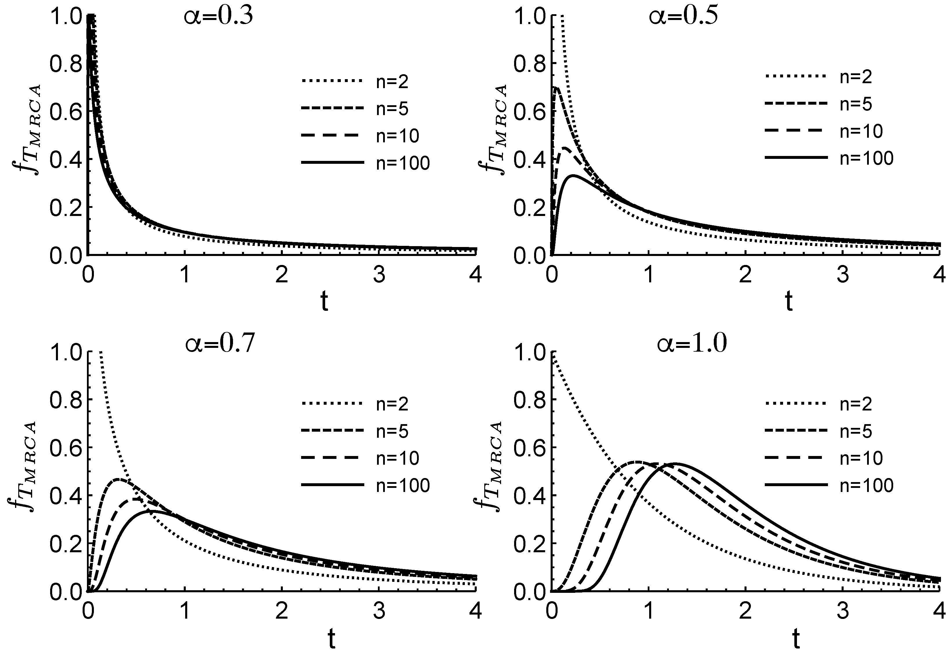
The key insight from [15] is that when the variance in offspring number is not constant—due, for example, to changing environmental conditions—the waiting time distribution becomes dependent on the order of the fractional derivative, denoted by $\alpha$. Figure 1 illustrates how changes in $\alpha$ affect the distribution of the time to the most recent common ancestor, $f_{T_{\mathrm{MRCA}}}\left(t\right)$. Here, $\alpha =1$ corresponds to no fluctuations, while smaller values of $\alpha$ indicate greater variability in offspring number. In this context, $\alpha$ serves as a measure of the intensity of fluctuations arising from heterogeneous environments. The figure assumes a population of size n.

In the fractional calculus framework, real datasets have also been analyzed, covering three species with distinct life history strategies: humpback whales, which are long-lived, highly mobile, and produce few offspring; the malaria parasite Plasmodium falciparum, which must adapt to both mosquito saliva and the vertebrate bloodstream; and influenza viruses, which face highly variable host immune responses, leading to considerable heterogeneity in transmission dynamics [15].

The analysis shows that environmental heterogeneity has minimal effect on the humpback whale and malaria parasite datasets. However, for the influenza dataset, heterogeneity appears to play a significant role and must be considered in population genetic inference. These findings emphasize that estimates of effective population size—and thus species diversity—can be strongly affected by whether heterogeneity is incorporated into the model [15].

In scenarios where gene frequency dynamics follow a Markov process, it has been shown that the average coalescent time equals the average fixation time [16,17,18]. Based on Figure 1, since coalescent time depends on the parameter $\alpha$, which reflects the intensity of fluctuations due to environmental heterogeneity, it follows that fixation time also depends on $\alpha$. In both the forward- and backward-time processes, $\alpha$ represents the order of the fractional derivative.

In the forward-time framework, this fractional order appears in the differential equation given in Equation (6). In this paper, we investigate how $\alpha$ influences fixation time by introducing a new numerical method for solving Equation (6). In future research, we plan to extend this analysis to real datasets to further explore the role of heterogeneity in evolutionary dynamics.

3. Eta-Based Functions

Eta functions were introduced by L. Gr. Ixaru [27], as a tool for deriving highly accurate CP methods for the Schrödinger equation. However, as was realized later on, they are of equal importance for the derivation by exponential fitting of numerical formulas for operations on highly oscillatory functions (numerical differentiation, quadrature, solving differential equations, interpolation, etc.); see [28,31,32,33,34,35,38,39] and references therein.

The Eta functions are primarily intended to approximate functions of the forms

$$F\left(t\right)={\Omega }_1\left(t\right)sin\left(\omega t\right)+{\Omega }_2\left(t\right)cos\left(\omega t\right)\mathrm{or}F\left(t\right)={\Omega }_1\left(t\right)sinh\left(\omega t\right)+{\Omega }_2\left(t\right)cosh\left(\omega t\right),$$

(8)

where frequency $\omega$ is a given constant, and ${\Omega }_1\left(t\right),{\Omega }_2\left(t\right)$ are smooth and slowly varying functions. With them, different categories of functions become tractable on equal footing. Thus, when $\omega$ is small, these functions are smooth, but when $\omega$ is increased, their behavior is increasingly oscillatory or with hyperbolic variation.

Eta functions ${\eta }_m\left(Z\right)$ with $m>0$ and $Z\ne 0$ are generated by recurrence [27,28]:

$${\eta }_m\left(Z\right)={\displaystyle \frac{{\eta }_{m-2}\left(Z\right)-(2m-1){\eta }_{m-1}\left(Z\right)}{Z}},m=1,2,3,\dots$$

(9)

where

$${\eta }_{-1}\left(Z\right)=\left\{\begin{array}{cc}cos\left(\right|Z{|}^{{\displaystyle \frac{1}{2}}})\hfill & Z\le 0\hfill \\ cosh\left(Z^{{\displaystyle \frac{1}{2}}}\right)\hfill & Z>0,\hfill \end{array}\right.{\eta }_0\left(Z\right)=\left\{\begin{array}{cc}{\displaystyle \frac{sin\left(\right|Z{|}^{\frac{1}{2}})}{{\left|Z\right|}^{\frac{1}{2}}}}\hfill & Z<0\hfill \\ 1\hfill & Z=0\hfill \\ {\displaystyle \frac{sinh\left(Z^{\frac{1}{2}}\right)}{Z^{\frac{1}{2}}}}\hfill & Z>0.\hfill \end{array}\right.$$

(10)

For $Z=0$ these functions have the following values:

$${\eta }_m\left(0\right)={\displaystyle \frac{1}{(2m+1)!!}},m=1,2,.\dots$$

(11)

where $!!$ is a double factorial [27]. These functions have the following property [24]:

$${\eta }_m\left(Z\right)=2^m\sum _{q=0}^{\infty }{\displaystyle \frac{(q+m)!}{q!(2q+2m+1)!}}{Z}^q=2^{-(m+1)}\sqrt{\pi }\sum _{q=0}^{\infty }{\displaystyle \frac{1}{\Gamma (q+m+\frac{3}{2})}}{\displaystyle \frac{{\left(\frac{Z}{4}\right)}^q}{q!}},m=0,1,\dots$$

(12)

These functions are used to introduce the set of Eta-based functions in the following way:

$$f_m\left(x\right)=x^{m-1}{\eta }_{\lfloor {\displaystyle \frac{m}{2}}\rfloor -1}\left(Z\left(x\right)\right),m=1,2,\dots$$

(13)

where $\lfloor {\displaystyle \frac{m}{2}}\rfloor$ is the integer part of ${\displaystyle \frac{m}{2}}$, and $Z\left(x\right)=-{\omega }^2{x}^2$ in the trigonometric case and $Z\left(x\right)={\omega }^2{x}^2$ in the hyperbolic case. An important property of the Eta-based functions is that they tend to power functions when $\omega =0$ (for more details, please see [28]).

3.1. Best Approximation Using Eta-Based Functions

Suppose that $H=L^2[0,1]$ and $\{f_1\left(x\right),f_2\left(x\right),\dots ,f_M\left(x\right)\}\subset H$ be the set of Eta-based functions and

$$Y=span\{f_1\left(x\right),f_2\left(x\right),\dots ,f_M\left(x\right)\}$$

and f is an arbitrary element in H. Because Y is a finite-dimensional vector space, f has the unique best approximation out of Y, such as $g\in Y,$ that is

$$\forall y\in Y,\Vert f-g\Vert \le \Vert f-y\Vert .$$

Since $g\in Y,$ there exist the unique coefficients $c_1,c_2,\dots ,c_M$, such that

$$f\simeq g=\sum _{m=1}^M{c}_m{f}_m\left(x\right)=C^{T}B\left(x\right),$$

(14)

where

$$B^T\left(x\right)=[f_1\left(x\right),f_2\left(x\right),\dots ,f_M\left(x\right)],$$

(15)

and

$$C^T=[c_1,c_2,\dots ,c_M].$$

(16)

Using the properties of the best approximation [40], because $f\in H$ using Equation (14), we have

$$f_i=<f,f_i\left(x\right)>=<\sum _{m=1}^M{c}_m{f}_m\left(x\right),f_i\left(x\right)>=\sum _{m=1}^M{c}_m{d}_m^i$$

$$i=1,2,\dots ,M,$$

where $f_i=<f,f_i\left(x\right)>$ and $d_m^i=<f_m\left(x\right),f_i\left(x\right)>$ and $<,>$ denote inner product.

Therefore

$$f_i=C^T{[d_1^i,d_2^i,\dots ,d_M^i]}^T.$$

$$i=1,2,\dots ,M.$$

So we get

$$F=D^{T}C,$$

where

$$F={[f_1,f_2,\dots ,f_M]}^T$$

and

$$D=\left[d_m^i\right]$$

where D is a dual operational matrix of order $M\times M$ and has the following definition:

$$D={\int }_0^{1}B\left(x\right)B^T\left(x\right)dx.$$

(17)

In the next section, we use matrix D to introduce the operational matrix of fractional derivatives of Eta-based functions.

3.2. Operational Matrix of Fractional Derivatives

In this section, we introduce the fractional derivative matrix of the Eta-based function. We use the series presentation of Eta-function in Equation (12) to derive the fractional derivative matrix.

Using Equation (15), the fractional derivative matrix is defined as

$$D_x^{\alpha }\left(B\left(x\right)\right)=H_{\alpha }B\left(x\right),$$

(18)

where $H_{\alpha }$ in the $M\times M$ derivative matrix. Using Equation (12) and the definition of the Caputo fractional derivative in Equation (5), the element of the matrix $H_{\alpha }$ is defined as

$$H_{\alpha }=\left[h_{ij}\right],i,j=1,2,\dots ,M,$$

(19)

where for the trigonometric and $i=1$ we have

$$h_{ij}=\sum _{q=1}^N{\displaystyle \frac{{(-1)}^q{\omega }^{2q}}{\left(2q\right)!}}{\displaystyle \frac{\Gamma (2q+1)}{\Gamma (2q+1-\alpha )}}{l}_{qj}^i,$$

and for $i\ne 1$ we have

$$h_{ij}=\sum _{q=0}^N{2}^{\lfloor {\displaystyle \frac{i}{2}}\rfloor -1}{\displaystyle \frac{(q+\lfloor \frac{i}{2}\rfloor -1)!}{q!(2q+2\lfloor \frac{i}{2}\rfloor -1)!}}{(-\omega )}^2{\displaystyle \frac{\Gamma (2q+i)}{\Gamma (2q+i-\alpha )}}{l}_{qj}^i,$$

also, for the hyperbolic case and $i=1$, we have

$$h_{ij}=\sum _{q=1}^N{\displaystyle \frac{{\omega }^{2q}}{\left(2q\right)!}}{\displaystyle \frac{\Gamma (2q+1)}{\Gamma (2q+1-\alpha )}}{l}_{qj}^i,$$

and for $i\ne 1$ we have

$$h_{ij}=\sum _{q=0}^N{2}^{\lfloor {\displaystyle \frac{i}{2}}\rfloor -1}{\displaystyle \frac{(q+\lfloor \frac{i}{2}\rfloor -1)!}{q!(2q+2\lfloor \frac{i}{2}\rfloor -1)!}}{\left(\omega \right)}^2{\displaystyle \frac{\Gamma (2q+i)}{\Gamma (2q+i-\alpha )}}{l}_{qj}^i,$$

and

$$l_{qj}^i=[{\int }_0^1{x}^{2q+i-1-\alpha }\times f_1\left(x\right)dx,{\int }_0^1{x}^{2q+i-1-\alpha }\times f_2\left(x\right)dx,\dots ,{\int }_0^1{x}^{2q+i-1-\alpha }\times f_M\left(x\right)dx]\times D^{-1},$$

where the matrix D has been introduced in Equation (17), and N is the order of the truncated series defined in Equation (12). In the next section, we use the operational matrix of fractional derivatives to introduce a numerical method for solving the fractional differential equation.

4. Numerical Method

In this section, we use the Eta-based function to solve the general fractional differential equation, which has the following form:

$$\begin{array}{c}M\left(x\right)D_x^{\alpha }f\left(x\right)+V\left(x\right)D_x^{2\alpha }f\left(x\right)+Q\left(x\right)=0,0\le \alpha \le 1,0\le x\le 1\hfill \\ \\ f\left(0\right)=f_0,f\left(1\right)=f_1,\hfill \end{array}$$

(20)

where $Q\left(x\right)$ is a known function.

Let us assume, using Equation (14), the best approximation of function $f\left(x\right)$ has the following form:

$$f\left(x\right)\simeq C^{T}B\left(x\right),$$

(21)

using Equations (21) and (18), we get

$$D_x^{\alpha }f\left(x\right)\simeq C^T{H}_{\alpha }B\left(x\right),D_x^{2\alpha }f\left(x\right)\simeq C^T{H}_{2\alpha }B\left(x\right),$$

(22)

Substitute Equations (21) and (22) in Equation (20), and we have

$$M\left(x\right)C^T{H}_{\alpha }B\left(x\right)+V\left(x\right)C^T{H}_{2\alpha }B\left(x\right)+Q\left(x\right)=0$$

(23)

We apply the collocation method by requiring the residual of the problem in Equation (23) to vanish at specific collocation points. These points are chosen as Newton–Cotes nodes $x_r$, given by [41]

$$x_r={\displaystyle \frac{r}{M}},r=1,\dots ,M-1.$$

(24)

To enforce the boundary conditions, we formulate the following optimization problem:

$$\begin{array}{cc}\mathrm{Minimize}\hfill & J={\sum }_{r=1}^{M-1}{(M\left(x_r\right)C^T{H}_{\alpha }B\left(x_r\right)+V\left(x_r\right)C^T{H}_{2\alpha }B\left(x_r\right)+Q\left(x_r\right))}^2,\hfill \\ \hfill & \\ \mathrm{subject}\mathrm{to}\hfill & C^{T}B\left(0\right)-f_0=0,\hfill \\ \hfill & \\ \hfill & C^{T}B\left(1\right)-f_1=0,\hfill \end{array}$$

(25)

Equation (25) defines a nonlinear programming problem, which can be solved using standard optimization techniques. In our implementation, we use Mathematica to solve for the unknown coefficient vector $C^T$.

4.1. Error Bound

This section aims to assess the error norm associated with the numerical scheme outlined in Section 4. To initiate the discourse on errors, we first introduce the following theorem, which serves as a foundation for the subsequent discussion in this section.

Theorem 1.

Suppose that $f\left(x\right)$ belongs to the Sobolev space $H^{\mu }(0,1)$ and $\mu \ge 0$, and $f_m(m=1,\dots ,M)$ are the Eta-based functions defined on the interval $[0,1]$. Assume that $g\left(x\right)=\sum _{m=1}^M{c}_m{f}_m\left(x\right)$ denotes the best approximation of a function $f\left(x\right)$. Then we have [42]

$${∥f\left(x\right)-g\left(x\right)∥}_{L^{\infty }(0,1)}\le c{M}^{{\displaystyle \frac{3}{4}}-\mu }{\left|f\right|}_{H^{\mu ;M}(0,1)}+\sum _{m=1}^M{2}^{-\lfloor {\displaystyle \frac{m}{2}}\rfloor }\sqrt{\pi }{\epsilon }_m\left|c_m\right|,$$

(26)

where ${\epsilon }_m$ is a small number depending on Eta-based functions, and

$${\left|f\right|}_{H^{\mu ;M}(0,1)}={\left(\sum _{r=min\{\mu ,M+1\}}^{\mu }{∥f^{\left(r\right)}∥}_{L^2(0,1)}^2\right)}^{{\displaystyle \frac{1}{2}}}.$$

In the next theorem, we will conduct an error analysis for the numerical scheme presented in Section 4.

Theorem 2.

Suppose that $f\left(x\right)$ belongs to the Sobolev space $H^{\mu }(0,1)$ and $\mu \ge 0$, and $f_m(m=1,\dots ,M)$ are the Eta-based functions defined on the interval $[0,1]$. Assume that $g\left(x\right)=\sum _{m=1}^M{c}_m{f}_m\left(x\right)$ denotes the best approximation of a function $f\left(x\right)$. Then

$$\left|\right|E_M{\left|\right|}_{L^{\infty }(0,1)}\le ({\displaystyle \frac{{\left|\right|M\left(x\right)\left|\right|}_{L^{\infty }(0,1)}}{\Gamma (2-\alpha )}}+{\displaystyle \frac{{\left|\right|V\left(x\right)\left|\right|}_{L^{\infty }(0,1)}}{\Gamma (3-2\alpha )}})(c{M}^{{\displaystyle \frac{3}{4}}-\mu }{\left|f\right|}_{H^{\mu ;M}}(0,1)+\sum _{m=1}^M{2}^{-\lfloor {\displaystyle \frac{m}{2}}\rfloor }\sqrt{\pi }{\epsilon }_m\left|c_m\right|),$$

where $E_M$ is the error bound.

Proof. 

If $g\left(x\right)$ is the best approximation of $f\left(x\right)$, using Equation (20), we have

$$\left|\right|E_M{\left|\right|}_{L^{\infty }(0,1)}=\left|\right|M\left(x\right)D^{\alpha }g\left(x\right)+V\left(x\right)D^{2\alpha }g\left(x\right)-Q\left(x\right){\left|\right|}_{L^{\infty }(0,1)}$$

$$=\left|\right|M\left(x\right)D^{\alpha }g\left(x\right)+V\left(x\right)D^{2\alpha }g\left(x\right)-(M\left(x\right)D^{\alpha }f\left(x\right)+V\left(x\right)D^{2\alpha }f\left(x\right)){\left|\right|}_{L^{\infty }(0,1)},$$

(27)

and using Equation (27), we have

$$\left|\right|E_M{\left|\right|}_{L^{\infty }(0,1)}\le {\left|\right|M\left(x\right)\left|\right|}_{L^{\infty }(0,1)}\left|\right|D^{\alpha }f\left(x\right)-D^{\alpha }g\left(x\right){\left|\right|}_{L^{\infty }(0,1)}+$$

$${\left|\right|V\left(x\right)\left|\right|}_{L^{\infty }(0,1)}\left|\right|D^{2\alpha }f\left(x\right)-D^{2\alpha }g\left(x\right){\left|\right|}_{L^{\infty }(0,1)}.$$

(28)

We assume $0\le \alpha <1$ and $1\le 2\alpha <2$, so we have [43]

$$\begin{array}{c}\left|\right|D^{\alpha }f\left(x\right)-D^{\alpha }g\left(x\right){\left|\right|}_{L^{\infty }(0,1)}\le {\displaystyle \frac{\left|\right|f\left(x\right)-{g\left(x\right)\left|\right|}_{L^{\infty }(0,1)}}{\Gamma (2-\alpha )}},\hfill \\ \left|\right|D^{2\alpha }f\left(x\right)-D^{2\alpha }g\left(x\right){\left|\right|}_{L^{\infty }(0,1)}\le {\displaystyle \frac{\left|\right|f\left(x\right)-{g\left(x\right)\left|\right|}_{L^{\infty }(0,1)}}{\Gamma (3-2\alpha )}}.\hfill \end{array}$$

(29)

Using Equations (26), (28), and (29), the result can be obtained. □

Remark 1.

The results of Theorem 2 show that the convergence rate depends not only on the number of basis functions but also on the order of the fractional derivatives, α. This contrasts with the classical spectral method for solving dynamical systems, where the convergence rate depends solely on the number of basis functions.

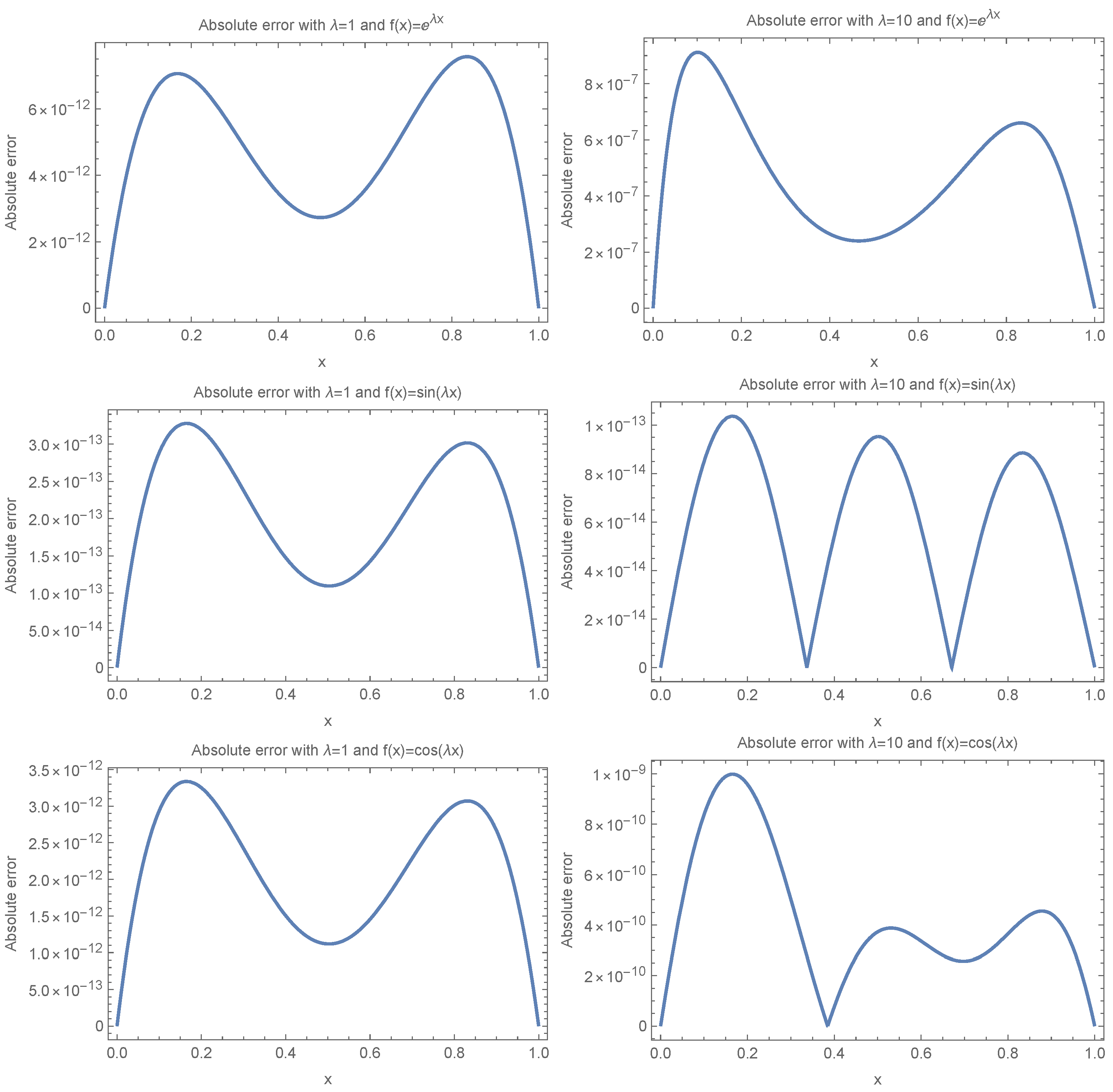
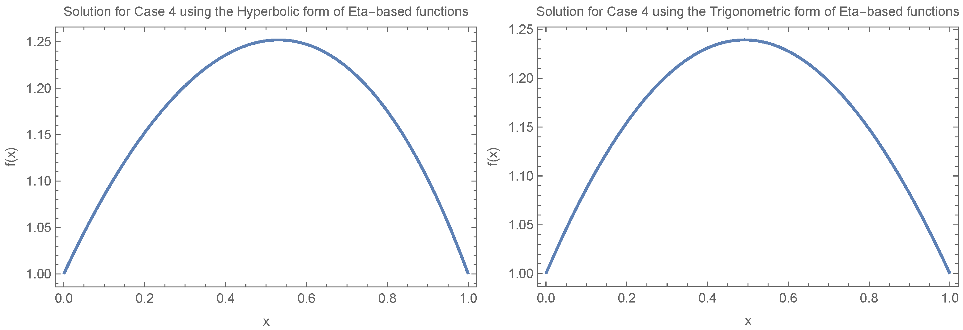
4.2. Numerical Example

In this section, we apply the numerical method introduced in Section 4 to solve a set of test cases and evaluate the accuracy of the approach. For the computations in this section, we used Mathematica 14.1.0 for Mac OS X $x86$ (64-bit) (16 July 2024). The reported error is the absolute error $L^{\infty }$, computed for different scenarios of the problems.

• Case 1: We consider Equation (20) with either $M\left(x\right)=1$, $V\left(x\right)=0$ or $M\left(x\right)=0$, $V\left(x\right)=1$, and choose $Q\left(x\right)$ such that the exact solution is $f\left(x\right)=e^{\lambda x}$. To provide more details, we first consider the case $M\left(x\right)=1$, $V\left(x\right)=0$. The other case, $M\left(x\right)=0$, $V\left(x\right)=1$, can be treated using a similar method. For $M\left(x\right)=1$, $V\left(x\right)=0$, Equation (20) takes the following form:

  $$\begin{array}{c}{D}_x^{\alpha }f\left(x\right)+Q\left(x\right)=0,0\le \alpha \le 1,0\le x\le 1\hfill \\ \\ f\left(0\right)=f_0,f\left(1\right)=f_1,\hfill \end{array}$$

  (30)
  Since the exact solution is $f\left(x\right)=e^{\lambda x}$, the function $Q\left(x\right)$ takes the following form:

  $$Q\left(x\right)=-\lambda t^{1-\alpha }\left({\mathcal{E}}_{1,2-\alpha }\left(\lambda t\right)\right)$$

  where ${\mathcal{E}}_{\alpha ,\beta }\left(t\right)$ denotes the Mittag–Leffler function, defined by the following expression:

  $${\mathcal{E}}_{\alpha ,\beta }\left(t\right)=\sum _{n=0}^{\infty }{\displaystyle \frac{t^n}{\Gamma (\alpha n+\beta )}},\alpha >0,\beta ,t\in \mathcal{C},$$

  (31)

  and ${\mathcal{E}}_{\alpha ,1}\left(t\right)={\mathcal{E}}_{\alpha }\left(t\right).$
  To apply the numerical method presented in Section 4, we use Equation (21) and assume $f\left(x\right)\simeq C^{T}B\left(x\right)$. Then, using Equations (25) and (30), we formulate the following optimization problem:

  $$\begin{array}{cc}\mathrm{Minimize}\hfill & J=\sum _{r=1}^{M-1}{(C^T{H}_{\alpha }B\left(x_r\right)+Q\left(x_r\right))}^2,\hfill \\ \hfill & \\ \mathrm{subject}\mathrm{to}\hfill & C^{T}B\left(0\right)-1=0,\hfill \\ \hfill & \\ \hfill & C^{T}B\left(1\right)-e^{\lambda }=0,\hfill \\ \hfill & \end{array}$$

  (32)

  where $x_r$ are chosen as the Newton–Cotes nodes, given in Equation (24).
  Equation (32) defines a nonlinear programming problem that can be solved using standard optimization techniques. In our implementation, we employ Mathematica to determine the unknown coefficient vector $C^T$.
  Figure 2 shows the results for $\alpha =1$ with various values of $\lambda$. The method demonstrates excellent performance, especially for large values of $\lambda$ (i.e., highly oscillatory cases), where classical basis functions typically struggle to maintain accuracy.

  Table 1. Absolute error for Case 1 with varying values of $\alpha$ and $\lambda$.

  Case 1	$\mathit{\lambda }=1$	$\mathit{\lambda }=3$	$\mathit{\lambda }=5$	$\mathit{\lambda }=7$
  $\alpha =0.2$	$6.0\times {10}^{-4}$	$25\times {10}^{-4}$	$14\times {10}^{-4}$	$6.0\times {10}^{-3}$
  $\alpha =0.8$	$25\times {10}^{-4}$	$4.0\times {10}^{-3}$	$5.0\times {10}^{-3}$	$15\times {10}^{-3}$

  presents the absolute error for different values of $\alpha$ and $\lambda$. These results indicate that even for $\alpha \ne 1$, the absolute error remains sufficiently small to support qualitative conclusions about fixation time behavior, which we explore in the next section.
• Case 2: Again using Equation (20) with $M\left(x\right)=1$, $V\left(x\right)=0$ or $M\left(x\right)=0$, $V\left(x\right)=1$, we now choose $Q\left(x\right)$ so that the exact solution is $f\left(x\right)=sin\left(\lambda x\right)$. The details for deriving the exact solution and applying the numerical method in this case are similar to those in Case 1.
  Figure 2 illustrates the results for $\alpha =1$ across various values of $\lambda$. As in Case 1, the method delivers high accuracy even for large $\lambda$, where oscillations typically hinder traditional methods.

  Table 2. Absolute error for Case 2 with varying values of $\alpha$ and $\lambda$.

  Case 2	$\mathit{\lambda }=1$	$\mathit{\lambda }=3$	$\mathit{\lambda }=5$	$\mathit{\lambda }=7$
  $\alpha =0.2$	$8.0\times {10}^{-4}$	$6.0\times {10}^{-4}$	$14\times {10}^{-4}$	$2.0\times {10}^{-3}$
  $\alpha =0.8$	$2.0\times {10}^{-3}$	$15\times {10}^{-3}$	$7.0\times {10}^{-3}$	$12\times {10}^{-3}$

  displays the absolute errors corresponding to different combinations of $\alpha$ and $\lambda$. For $\alpha \ne 1$, the errors remain sufficiently low to inform our discussion of fixation time behavior in the following section.
• Case 3: We now consider Equation (20) with $M\left(x\right)=1$, $V\left(x\right)=0$ or $M\left(x\right)=0$, $V\left(x\right)=1$, selecting $Q\left(x\right)$ such that the exact solution is $f\left(x\right)=cos\left(\lambda x\right)$. The details for deriving the exact solution and applying the numerical method in this case are similar to those in Case 1. Figure 2 presents the results for $\alpha =1$ and a range of $\lambda$ values. Once again, the method performs reliably, maintaining high accuracy even for large $\lambda$ and outperforming traditional approaches for oscillatory solutions.

  Table 3. Absolute error for Case 3 with varying values of $\alpha$ and $\lambda$.

  Case 3	$\mathit{\lambda }=1$	$\mathit{\lambda }=3$	$\mathit{\lambda }=5$	$\mathit{\lambda }=7$
  $\alpha =0.2$	$6.0\times {10}^{-5}$	$10\times {10}^{-4}$	$15\times {10}^{-4}$	$6.0\times {10}^{-3}$
  $\alpha =0.8$	$4.0\times {10}^{-5}$	$1.0\times {10}^{-4}$	$3.0\times {10}^{-4}$	$1.0\times {10}^{-3}$

  shows the absolute error for various values of $\alpha$ and $\lambda$. The results confirm that the method remains robust for $\alpha \ne 1$, providing a reliable basis for interpreting the fixation time behavior discussed in the next section.
• Case 4: We now consider Equation (20) with $M\left(x\right)=V\left(x\right)=Q\left(x\right)=1$, for which the exact solution is unknown. The numerical procedure follows that of Case 1. To assess robustness, we use Eta-based functions in both the trigonometric and hyperbolic forms. As shown in Figure 3, the solutions from both cases exhibit nearly identical behavior, with an error bound of about ${10}^{-3}$. This consistency indicates that Eta-based functions are reliable even without a known exact solution, supporting their use in studying fixation time behavior in Section 5, where the exact solution is also unavailable.

4.3. Advantages of Eta-Based Functions

In this section, to demonstrate the advantages of using Eta-based functions, we revisit two important cases from the previous section (Cases 2 and 3). We apply the same numerical method introduced in Section 4, but this time using Legendre polynomials, and compare the results with those obtained using Eta-based functions.

Table 4. Absolute error of Case 2 using Eta-based functions and Legendre polynomials for different values of $\lambda$.

Method	$\mathit{\lambda }=1$	$\mathit{\lambda }=5$	$\mathit{\lambda }=10$	$\mathit{\lambda }=15$
Eta-based functions	$3.0\times {10}^{-13}$	$8.0\times {10}^{-13}$	$1.0\times {10}^{-13}$	$5.0\times {10}^{-11}$
Legendre polynomials	$1.4\times {10}^{-6}$	$3.5\times {10}^{-2}$	$1.2\times {10}^0$	$2.5\times {10}^0$

and

Table 5. Absolute error of Case 3 using Eta-based functions and Legendre polynomials for different values of $\lambda$.

Method	$\mathit{\lambda }=1$	$\mathit{\lambda }=5$	$\mathit{\lambda }=10$	$\mathit{\lambda }=15$
Eta-based functions	$3.5\times {10}^{-12}$	$1.5\times {10}^{-16}$	$1.0\times {10}^{-9}$	$7.0\times {10}^{-16}$
Legendre polynomials	$2.5\times {10}^{-6}$	$2.5\times {10}^{-2}$	$1.5\times {10}^0$	$7.0\times {10}^0$

present the absolute errors for both Eta-based functions and Legendre polynomials, using the same number of basis functions ($M=5$), across different values of $\lambda$. The results align with those reported in [23], highlighting the superior performance of Eta-based functions over traditional basis functions such as Jacobi polynomials, especially in highly oscillatory regimes.

To provide a layman’s interpretation, the absolute errors reported in Table 4 and Table 5 measure how far the numerical results deviate from the expected or exact fixation time. For example, an error of ${10}^{-3}$ corresponds to a deviation of less than $0.1\%$ from the expected value, while an error of ${10}^{-6}$ reflects a deviation of less than $0.0001\%$. In our results, the Eta-based functions consistently produce errors on the order of ${10}^{-13}$ to ${10}^{-16}$, which implies extremely high accuracy—essentially, the results are accurate to more than 12 decimal places. In contrast, Legendre polynomials yield errors ranging from ${10}^{-6}$ to as high as ${10}^0$, which can mean deviations of $100\%$ or more in some cases. This stark contrast illustrates that using traditional basis functions like Legendre polynomials can lead to substantial inaccuracies, particularly for larger values of $\lambda$, which correspond to more oscillatory behavior in the solution. In practical terms, this means that models relying on Legendre polynomials may significantly misestimate fixation time in complex or rapidly changing environments, while Eta-based functions maintain reliable precision even under such challenging conditions.

5. Fixation Times in Population Genetics

In this section, we apply the numerical method presented in Section 4 to solve Equation (6), which presented the fixation time. This will help us study the behavior of fixation time in different scenarios. Using Equations (6), (21), and (22), we have

$$E\left(\delta x\right){\displaystyle \frac{C^T{H}_{\alpha }B\left(x\right)}{\Gamma (\alpha +1)}}+E{\left(\delta x\right)}^2{\displaystyle \frac{C^T{H}_{2\alpha }B\left(x\right)}{\Gamma (2\alpha +1)}}+1=0$$

(33)

We apply the collocation method by requiring the residual of the problem in Equation (33) to vanish at Newton–Cotes nodes $x_r$ in Equation (24). To enforce the boundary conditions in Equation (7) and ensure that the fixation time remains non-negative, we formulate the following optimization problem:

$$\begin{array}{cc}\mathrm{Minimize}\hfill & J={\sum }_{r=1}^{M-1}{(E\left(\delta x_r\right){\displaystyle \frac{C^T{H}_{\alpha }B\left(x_r\right)}{\Gamma (\alpha +1)}}+E{\left(\delta x_r\right)}^2{\displaystyle \frac{C^T{H}_{2\alpha }B\left(x_r\right)}{\Gamma (2\alpha +1)}}+1)}^2,\hfill \\ \hfill & \\ \mathrm{subject}\mathrm{to}\hfill & C^{T}B\left(0\right)-{\rho }_0=0,\hfill \\ \hfill & \\ \hfill & C^{T}B\left(1\right)-{\rho }_1=0,\hfill \\ \hfill & \\ \hfill & C^{T}B\left(x_r\right)\ge 0,r=1,\dots ,M-1.\hfill \end{array}$$

(34)

Equation (34) defines a nonlinear programming problem, which can be solved using standard optimization techniques. In our implementation, we use Mathematica to solve for the unknown coefficient vector $C^T$.

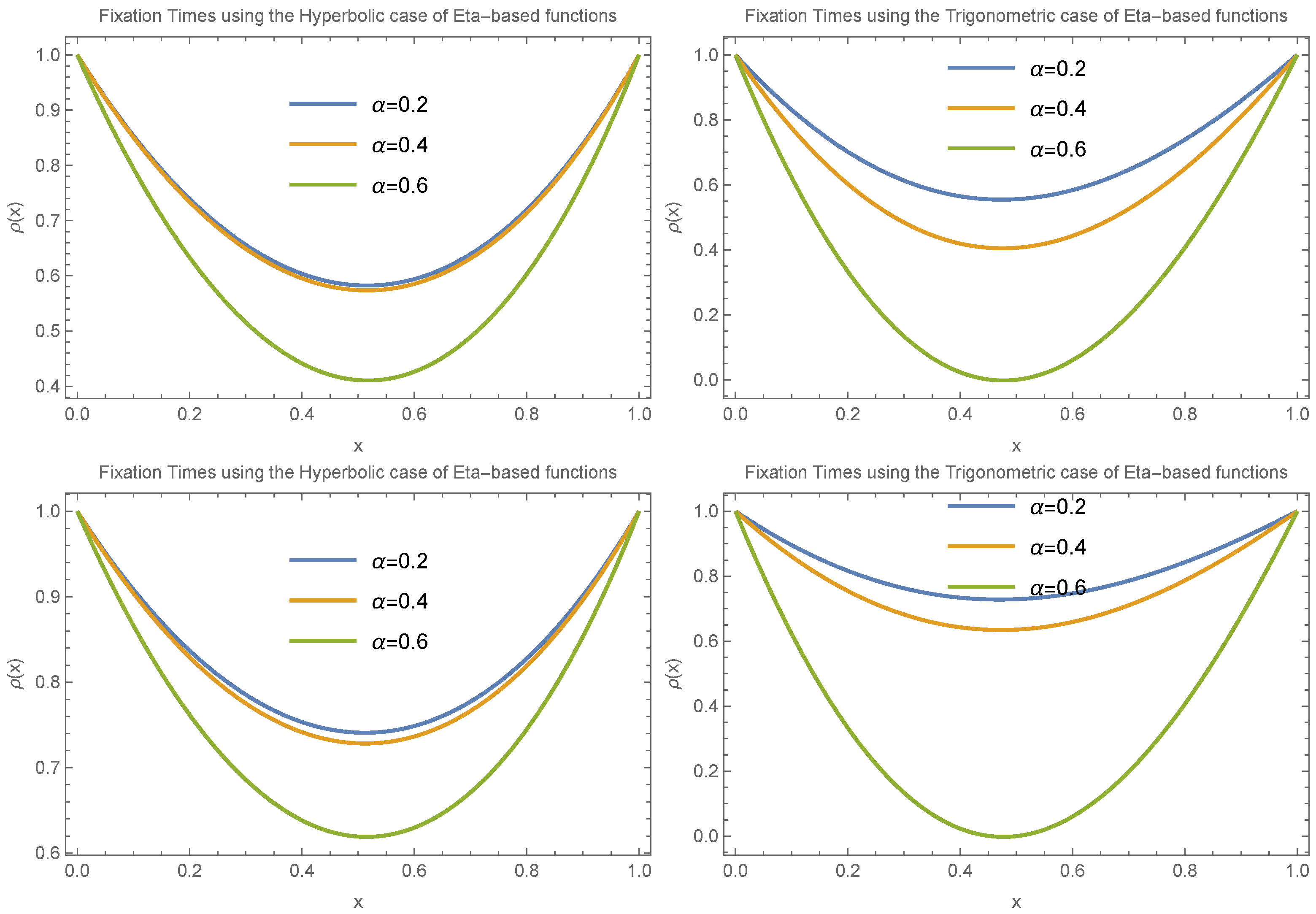
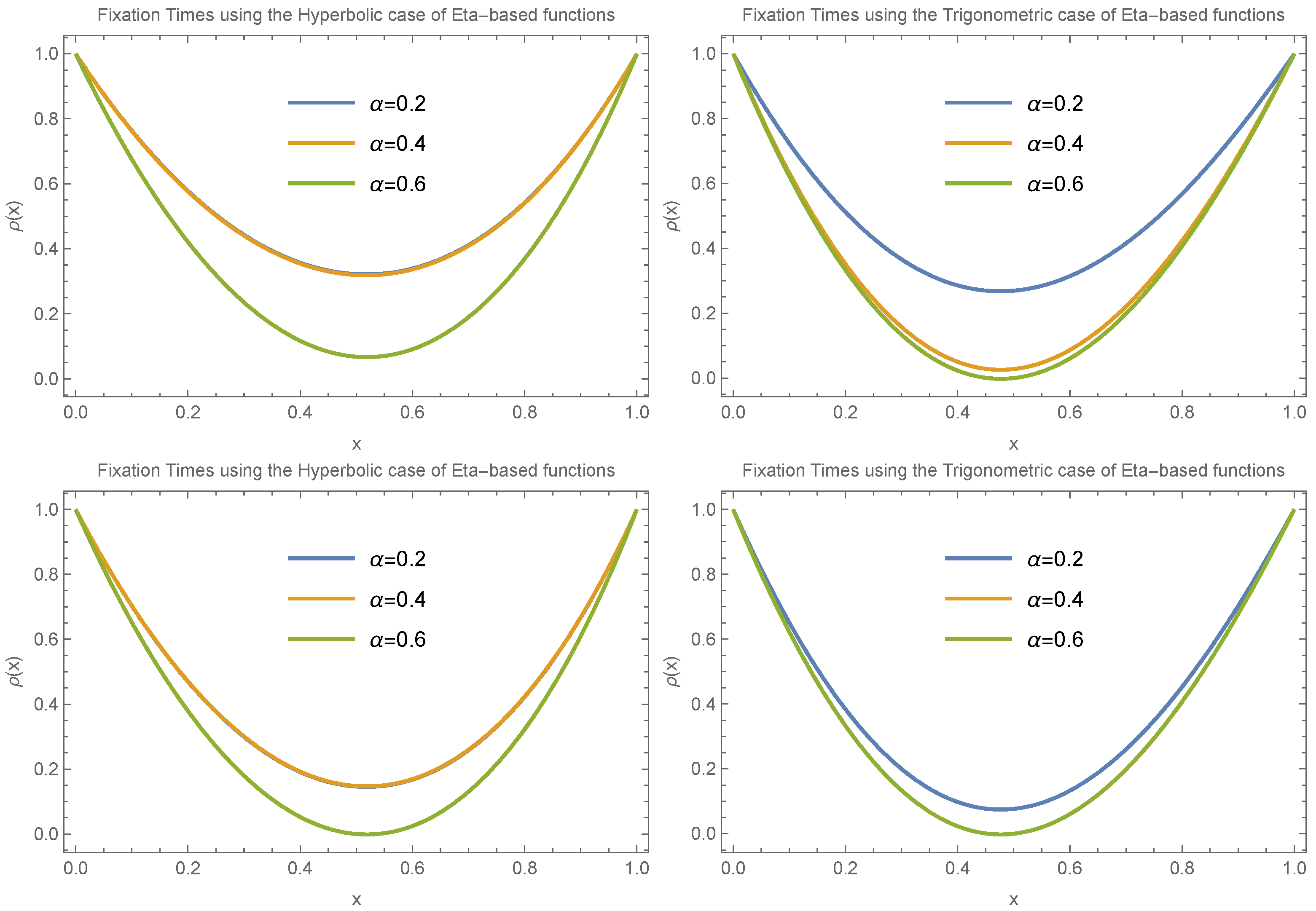
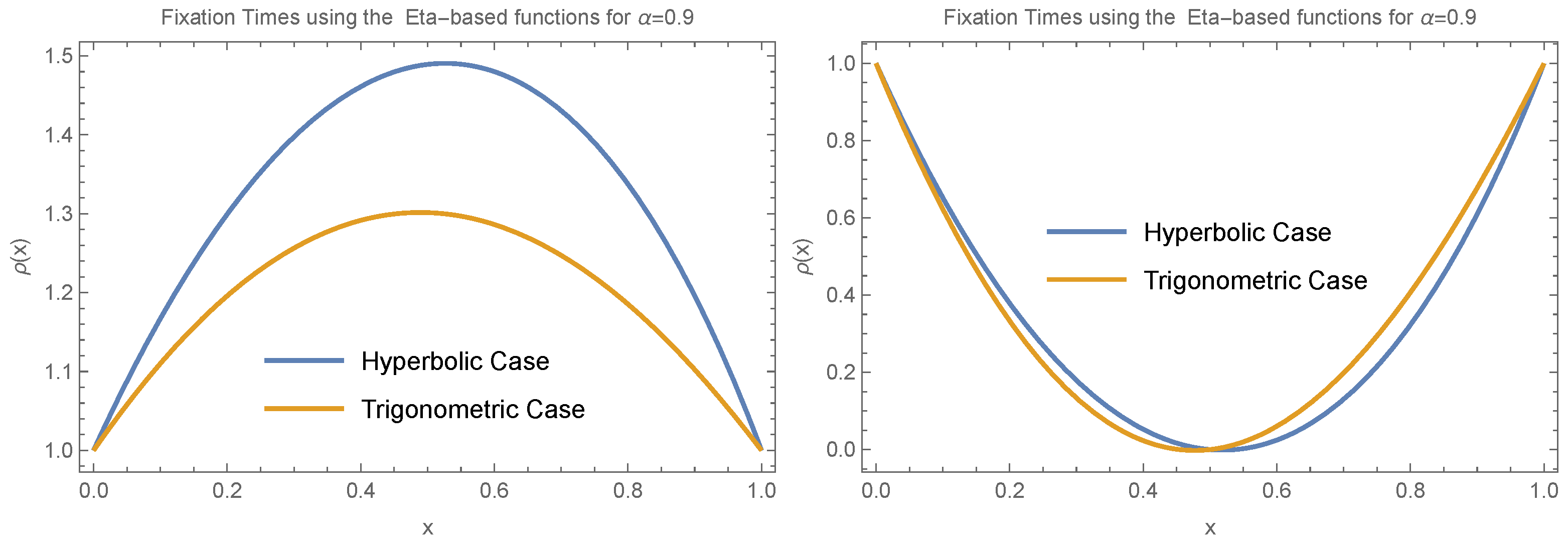
We explored several scenarios to study the behavior of the fixation time across different values of $\alpha$, which we interpret as a parameter reflecting the effect of heterogeneity. These scenarios involved varying the behavior of $E\left(\delta x\right)$ and $E{\left(\delta x\right)}^2$ by considering different functional forms for $E\left(\delta x_r\right)$ and $E{\left(\delta x_r\right)}^2$. Additionally, we examined different forms of the Eta functions, including both trigonometric and hyperbolic cases.

Figure 4 illustrates how fixation time changes with allele frequency x under the condition $E\left(\delta x\right)=E{\left(\delta x\right)}^2$. We consider two specific cases: $E\left(\delta x\right)=E{\left(\delta x\right)}^2=1$ and $E\left(\delta x\right)=E{\left(\delta x\right)}^2=e^x$, evaluating both the trigonometric and hyperbolic forms of the Eta function separately and focusing on small values of $\alpha$ ($\alpha <0.8$).

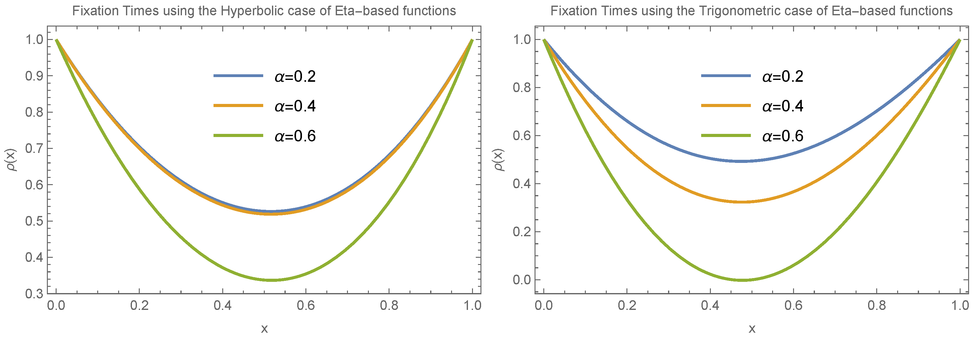
Figure 5 and Figure 6 continue with the assumption $E\left(\delta x\right)=E{\left(\delta x\right)}^2$ under different scenarios, including $E\left(\delta x\right)=E{\left(\delta x\right)}^2=e^{-x}$, $E\left(\delta x\right)=E{\left(\delta x\right)}^2=sin\left(x\right)$, and $E\left(\delta x\right)=E{\left(\delta x\right)}^2=cos\left(x\right)$, again for small $\alpha$ values ($\alpha <0.8$). The results in Figure 4, Figure 5 and Figure 6 show that despite the different scenarios, fixation time consistently decreases for small allele frequencies ($x<{\displaystyle \frac{1}{2}}$) and increases for large allele frequencies ($x>{\displaystyle \frac{1}{2}}$).

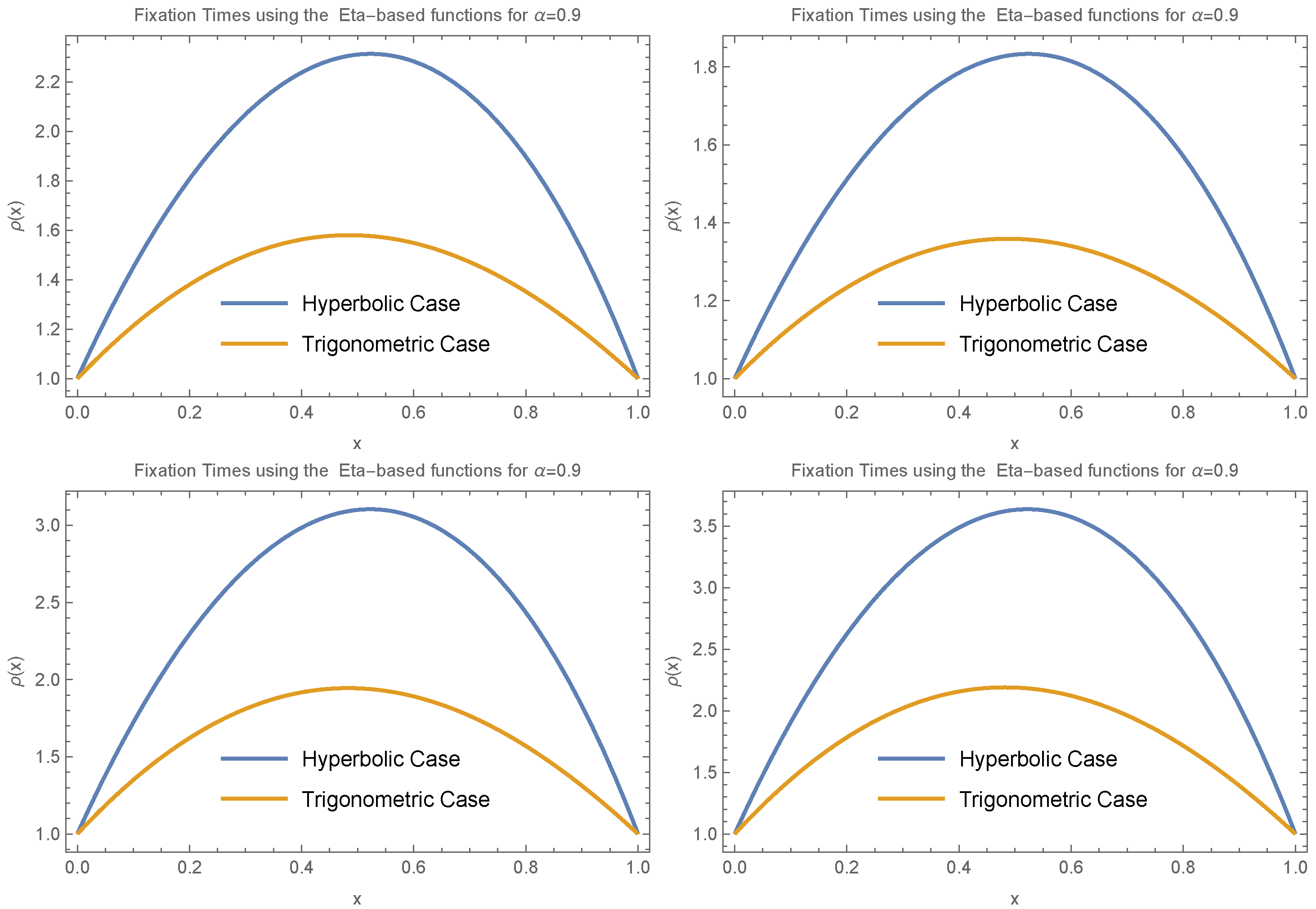
We also investigated the behavior of fixation time for a larger value of $\alpha$, specifically $\alpha =0.9$. In this case, we again assumed $E\left(\delta x\right)=E{\left(\delta x\right)}^2$ and explored several functional forms: $E\left(\delta x\right)=E{\left(\delta x\right)}^2=1$, $e^x$, $e^{-x}$, and $sin\left(x\right)$. The results, presented in Figure 7, include both trigonometric and hyperbolic forms of the Eta function. These results reveal that fixation time increases for small allele frequencies ($x<{\displaystyle \frac{1}{2}}$) and decreases for large allele frequencies ($x>{\displaystyle \frac{1}{2}}$).

Taken together, the results from Figure 4, Figure 5, Figure 6 and Figure 7 show that when $E\left(\delta x\right)=E{\left(\delta x\right)}^2$, the behavior of fixation time is qualitatively similar across different functional forms. For both small ($\alpha <0.8$) and large ($\alpha >0.8$) values of $\alpha$, fixation time tends to exhibit an extremum around $x={\displaystyle \frac{1}{2}}$.

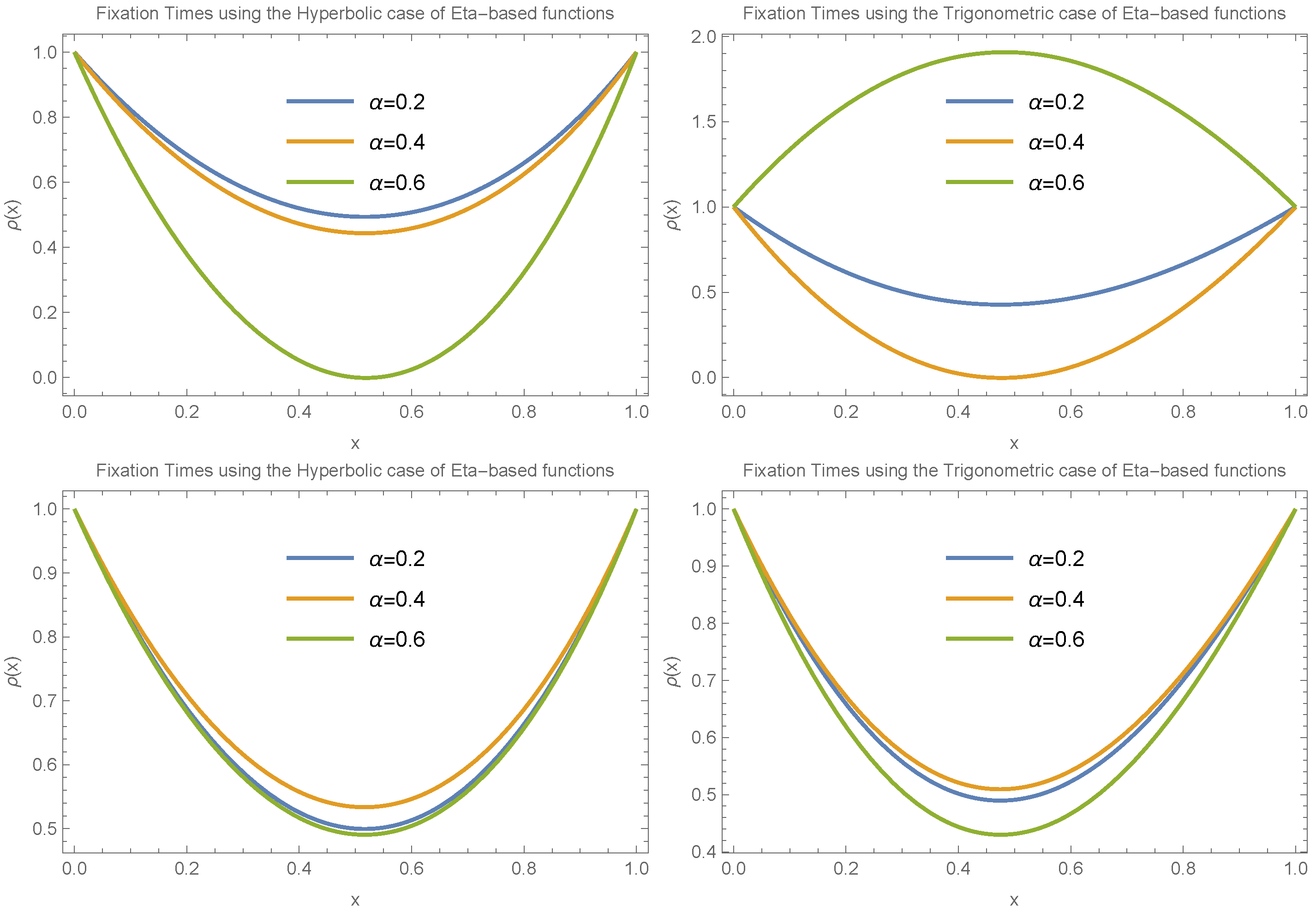
To draw a more general conclusion, we also considered the case where $E\left(\delta x\right)\ne E{\left(\delta x\right)}^2$. Figure 8 and Figure 9 present the results for small and large values of $\alpha$, respectively. These scenarios involve different choices for $E\left(\delta x\right)$ and $E{\left(\delta x\right)}^2$ in both trigonometric and hyperbolic Eta cases. The results again confirm the presence of an extremum in fixation time near $x={\displaystyle \frac{1}{2}}$. The main difference in this case is that the transition between having a minimum versus a maximum at the extreme point occurs more gradually compared to the $E\left(\delta x\right)=E{\left(\delta x\right)}^2$ case.

The numerical results show that fixation time depends on both the heterogeneity parameter $\alpha$ and the initial allele frequency. This contrasts with the classical approach, where heterogeneity is not considered and fixation time depends solely on the initial allele frequency. Specifically, for small values of $\alpha$, fixation time consistently decreases when the allele starts at low frequencies and increases when it starts at high frequencies. In contrast, for larger values of $\alpha$, this pattern may reverse, with fixation time increasing for low initial frequencies and decreasing for high ones. Biologically, this suggests that heterogeneity interacts with the initial genetic composition of the population in shaping allele dynamics. In microbial populations, where beneficial mutations typically arise at low frequencies, a highly heterogeneous environment (corresponding to small $\alpha$) may lead to more rapid fixation and faster adaptation. In more homogeneous settings, however, such mutations may take longer to fix unless they reach a higher frequency early in the process. Similarly, in tumor evolution, resistance mutations that appear at low frequencies may fix more rapidly in a heterogeneous tumor microenvironment, potentially reducing the window of opportunity for effective treatment. In contrast, a more uniform microenvironment may slow down this process unless resistant clones grow sufficiently large. These results indicate that our framework captures nuanced dynamics that are directly relevant to real-world evolutionary scenarios, particularly in systems where spatial or environmental heterogeneity plays a critical role.

6. Conclusions

In this study, we introduced a novel forward-time framework for estimating fixation time in population genetics by incorporating the effects of environmental heterogeneity using fractional calculus. Traditional models, such as the Wright–Fisher and classical coalescent approaches, assume uniform environments and equal reproductive success, which limits their ability to capture the complexity of real-world biological systems. By introducing a fractional parameter $\alpha$, our model explicitly accounts for the impact of heterogeneous environments on reproductive dynamics.

To solve the resulting fractional differential equations, we developed a spectral method based on Eta-based functions. These functions proved highly effective in approximating unknown or oscillatory solutions, enabling a computationally efficient and accurate numerical approach. By leveraging the operational matrix of fractional derivatives, we reduced the problem to an optimization framework, making the method scalable and practical for large systems.

Our numerical results demonstrated the consistency and robustness of the method across different parameter settings and basis functions, validating its utility in modeling fixation dynamics under varying degrees of heterogeneity. However, as with all modeling approaches, certain limitations should be noted. The current model assumes constant environmental heterogeneity over time and does not yet account for spatial structure, stochasticity, or gene flow. Addressing these factors could further enhance the model’s applicability and realism.

Despite these limitations, the proposed framework offers promising avenues for real-world applications. In particular, it may be relevant for modeling microbial adaptation in fluctuating environments, understanding clonal dynamics in cancer genomics where selection pressures vary across tissues, or exploring fixation processes in epidemiological contexts involving heterogeneous host immunity or transmission rates.

Overall, this work contributes both theoretical and computational advances toward understanding fixation time in heterogeneous populations, and it opens up several directions for future research in applied evolutionary modeling.