Abstract
Transfinite interpolation, originally proposed in the early 1970s as a global interpolation method, was first implemented using Lagrange polynomials and cubic Hermite splines. While initially developed for computer-aided geometric design (CAGD), the method also found application in global finite element analysis. With the advent of isogeometric analysis (IGA), Bernstein–Bézier polynomials have increasingly replaced Lagrange polynomials, particularly in conjunction with tensor product B-splines and non-uniform rational B-splines (NURBSs). Despite its early promise, transfinite interpolation has seen limited adoption in modern CAD/CAE workflows, primarily due to its mathematical complexity—especially when blending polynomials of different degrees. In this context, the present study revisits transfinite interpolation and demonstrates that, in four broad classes, Lagrange polynomials can be systematically replaced by Bernstein polynomials in a one-to-one manner, thus giving the same accuracy. In a fifth class, this replacement yields a robust dual set of basis functions with improved numerical properties. A key advantage of Bernstein polynomials lies in their natural compatibility with weighted formulations, enabling the accurate representation of conic sections and quadrics—scenarios where IGA methods are particularly effective. The proposed methodology is validated through its application to a boundary-value problem governed by the Laplace equation, as well as to the eigenvalue analysis of an acoustic cavity, thereby confirming its feasibility and accuracy.
Keywords:
transfinite interpolation; tensor product; Bernstein polynomials; Lagrange polynomials; isogeometric analysis (IGA); boundary-value problem (BVP); eigenvalue problem; finite element analysis MSC:
65B99; 65N06; 74S05
1. Introduction
Engineering analysis of two- and three-dimensional boundary-value (including eigenvalue) problems is usually performed using tensor product expansion of the problem variable, applying either local or global interpolation. In chronological sequence, from oldest to the most recent, the most-used univariate functions are Lagrange polynomials, Bernstein polynomials, B-splines, and NURBSs ([1,2,3], among others). And since these univariate functions are constituent elements of usual tensor products, they have successively passed from tensor product Lagrange polynomials to tensor product NURBS.
It is well known that Lagrange and Bernstein polynomials of the same degree n both form bases for the degree-n polynomial space and are thus linearly equivalent. The transformation between these bases dates back to 1932 [4] and is extensively covered in Lorentz’s classical monograph on Bernstein polynomials [5]. Subsequent research has explored their interrelations [6], the eigenstructure of Bernstein operators [7], and mappings via generalized Bézier curves [8]. Studies have also examined the asymptotic behavior of iterated Bernstein operators [9] and developed algorithms for converting between Bernstein and Lagrange forms [10].
In addition to the algebraic properties of Bernstein-type bases, considerable attention has been devoted to spline-based approximation frameworks, especially those emphasizing structural or geometric preservation. For instance, the construction and efficient computation of cardinal B-splines, which are foundational to many spline-based methods, have been studied in [11]. Subdivision schemes, which play a crucial role in geometric modeling and are intimately connected with B-spline refinement, are surveyed comprehensively in [12]. Shape-preserving approximations by polynomials and splines, which are essential in applications demanding monotonicity or convexity constraints, are developed in [13]. Similarly, moment-preserving spline approximations—vital for maintaining integral properties of the original function—are explored in [14,15]. A detailed and unified treatment of such topics, including both classical and modern developments in Bernstein operators and their applications, is presented in a recent monograph by Bustamante [16].
In the advent of isogeometric analysis (IGA), Lagrange polynomials have been progressively substituted by Bernstein polynomials as well as B-splines and NURBSs. One practical reason for this replacement is because the Bernstein polynomials allow for the introduction of weights that may ensure the accurate representation of conics and surfaces such as cylindrical and spherical parts [3]. However, this can be achieved not only for IGA tensor products but for transfinite patches as well [17]. Regarding the analysis module, which refers to the numerical solution to a partial differential equation (PDE) with given boundary conditions, the isoparametric concept has been adopted in all cases, which uses the same set of basis functions for the approximation of the geometry and the primary variable of the problem . In some simple cases, such as ideal tensor products implemented with Lagrange polynomials, the nodal values ’s can be blindly replaced by generalized coefficients denoted and the Lagrange by Bernstein polynomials [17,18], but the range of applicability of this method is still unknown.
For the sake of clarity and focus, this paper restricts itself to the use of Bernstein polynomials only, excluding discussions of B-splines and NURBSs. Overall, five categories of transfinite elements are investigated, as follows:
- Tensor product elements.
- Classical transfinite elements (fully structured).
- Distorted tensor products.
- Elements with different degrees on opposite edges (partially unstructured).
- Coons elements.
The study opens with a review of the tensor product formulation, leading to the derivation of a general transformation matrix that maps Lagrange polynomials to their Bernstein counterparts. This matrix is subsequently employed to establish the relationship between the nodal values and the generalized coefficients .
Next, the paper examines classical transfinite elements in a structured setting, where it uncovers the implicit transformation matrix governing the interpolation. It then extends the analysis to tensor product elements with distorted boundaries, identifying the relationship between nodal points and control points for both Lagrange and Bernstein representations.
The fourth part investigates non-tensor product elements, characterized by variable polynomial interpolation orders along their four edges. For these cases, a robust Bernstein-based basis is proposed, and avenues for future research are discussed. Finally, the paper presents a variation of the transfinite element inspired by the Coons patch, wherein nodal or control points are defined solely along the boundary.
The proposed methodology is validated through two benchmark problems: a boundary-value problem governed by the Laplace equation, and an acoustic eigenvalue problem. Both cases possess known closed-form solutions, allowing for rigorous accuracy assessment.
2. Basic Theory
2.1. Bernstein Polynomials
It is well known that the Bézier interpolation of a curve of degree n, or a univariate function, has the following form:
with the Bernstein polynomials given by
where gives the control points. In the case of a univariate function , the control points are substituted by the generalized coefficients .
2.2. Relationship Between Bernstein and Lagrange Polynomials
2.2.1. Univariate Approximation
Previously, in References [17,18,19], transformation matrices were derived that relate Lagrange polynomials to Bernstein polynomials of the same degree, . In more detail, if the x-axis is uniformly subdivided into m segments, the -associated Lagrange polynomials (of degree m) form a column vector , whereas the -associated Bernstein polynomials form another column vector . These two sets of polynomials of the same degree m are interrelated by
where is a transformation matrix of size .
2.2.2. Tensor Products
Similar expressions may be written also for the y-direction, where the corresponding column vectors ) and the associated transformation matrix appear:
In case of a tensor product of degree , using and nodal points along the axes x and y, respectively (i.e., totally nodal points), we can write the following (see [18]):
where the matrix of generalized coefficients (in tensor product Bernstein polynomials) is related to the matrix (including all the nodal values) through two univariate transformation matrices. These matrices are as follows:
and
An implementation of Equation (6) featuring a nine-node tensor product element is demonstrated in Section 3.5.
2.3. Non-Uniform Lagrange Polynomials
The standard expressions for the transformation matrices , as reported in prior studies [17,18,19], have been derived under the assumption of uniform (equally spaced) Lagrange polynomials. However, when the internal nodes along a parametric line segment (typically defined over the interval ) are displaced from their initial uniform positions, the underlying set of nodal points—on which the Lagrange basis is constructed—changes accordingly, since the nodal values are directly tied to those positions. In contrast, Bernstein polynomials maintain a fixed, standard form (as defined in Equation (1)) and are independent of the spatial distribution of the associated control points.
As a result, any modification to the nodal distribution along a segment leads to a corresponding change in the transformation matrix (e.g., or ) and, consequently, in the associated generalized coefficients. A numerical estimation of each one-dimensional transformation matrix—say, —can be performed by collocating Equation (5) at all nodal points over the interval , leading to the linear system . For each distinct configuration of internal nodal positions that defines the vector (of size , the matrix (of size ) changes accordingly. The coefficient vector is then obtained by inversion as , yielding the transformation matrix .
The case of multiple nodes is not examined in the present paper.
3. Transformation Matrices Between Tensor Product Bernstein and Lagrange Functional Sets
In this section, we shall derive the general expression for the transformation matrix , which correlates the tensor product Bernstein and Lagrange polynomial sets. For this purpose, as an example, first we start with the quadratic interpolation, and then we present the general expression.
3.1. Quadratic Interpolation
Let us consider a quadratic element (1-2-3) shown in Figure 1a. As has been proven previously in Ref. [18], the relationship between the three quadratic Lagrange polynomials associated with the nodes (1, 2, 3) and the corresponding Bernstein polynomials is as follows:
Note that regarding the subscripts in both polynomials of Equation (8), i.e., and , the first index ‘’ refers to the serial number of the node (measured from the left end) whereas the second index ‘’ (after comma) refers to the polynomial degree (here, ).

Figure 1.
(a) Quadratic and (b) bi-quadratic uniform elements.
Obviously, since each boundary edge of the bi-quadratic quadrilateral element shown in Figure 1b is entirely self-contained, the relationship given in Equation (8) is useful for interpolation along the horizontal edges towards the -direction (1-2-3 and 7-8-9). Moreover, regarding the vertical -direction, the independent variable in both parts of Equation (8) must be substituted by the independent variable .
To derive the bivariate shape functions of the element in Figure 1b, both parts of Equation (8) are multiplied by , which in turn is further replaced by the same transformation in , and thus we obtain the following:
whence we have
In a similar way, multiplying Equation (8) by , we obtain a shorter expression:
Also, multiplying Equation (8) by , we have
If all the nine shape functions of each functional set are packed into two column vectors as
then the combination of Equations (10)–(13) determines a linear relationship between them—i.e.,
with
3.2. Generalization
It is worth mentioning that in the general case of a ‘square’ tensor product associated with a univariate transformation matrix (with common entries ),
the transformation matrix may be written as follows:
Moreover, in the most general case of a ‘rectangular’ tensor product of degree associated with univariate transformation matrices with entries and with entries , the transformation matrix may be written as follows:
3.3. Transformation of Structural Engineering Matrices (K,M)
When the stiffness (and mass) matrix is known in the functional system of Lagrange polynomials, it is also known in terms Bernstein polynomials. In this context, omitting the corresponding factor (e.g., the density in elastodynamics, or the inverse of speed squared in acoustics), the mass matrix ( in the Lagrangian basis and in the Bézierian one) will be interrelated through the abovementioned transformation matrix , one being a quadratic form of the other, as follows:
In a similar way, the stiffness matrices in the two systems will be interrelated by
whereas, by virtue of Equation (14), the force vectors will be interrelated by
Considering a static problem, for the functional set including Lagrange polynomials, the equilibrium equation becomes
and by virtue of Equations (20) and (21) becomes
After simplification of matrix in both parts of Equation (23), we obtain the following:
Moreover, since the displacement field does not depend on the functional basis but is the same in both of them, we have
Substitution of Equation (14) into Equation (25) gives the following:
Substituting Equation (26) into Equation (24), we receive
| Significant Remark: Comparing the equilibrium equations in terms of Lagrange polynomials according to Equation (22) with those in terms of Bernstein polynomials according to Equation (27), one may understand that the numerical solution of each of them equals the numerical solution of the other. Similar findings regarding the equivalence of the two polynomial bases may be derived for the eigenvalue problem and transient analysis as well. |
3.4. Numerical Verification
In addition to the above theoretical presentation, we also demonstrate the numerical coincidence (and a small difference regarding the condition number) in the following BVP (Example 1), which is characterized by different polynomial degrees in each direction and a non-polynomial exact solution.
Example 1.
Heat-flow in rectangular domain.
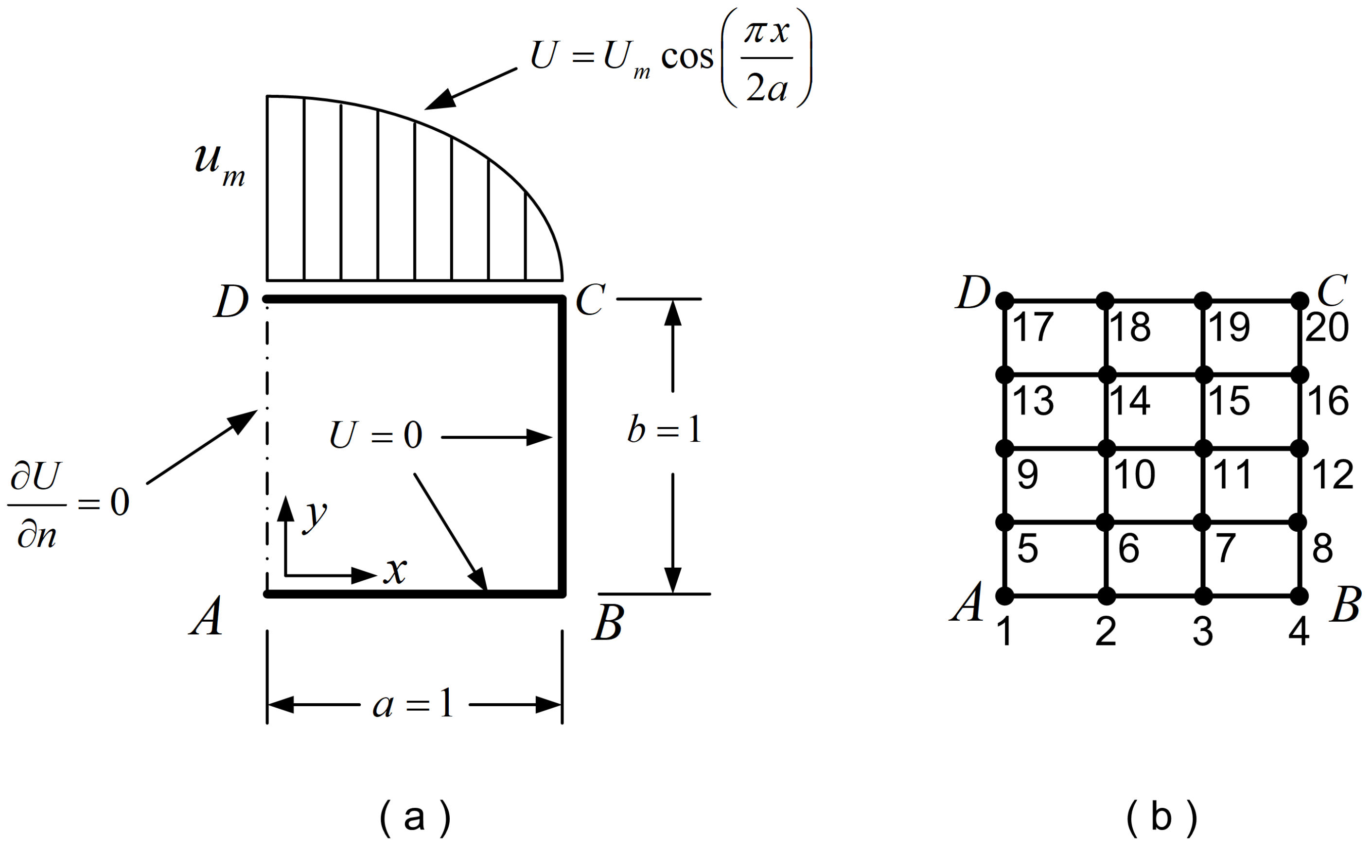
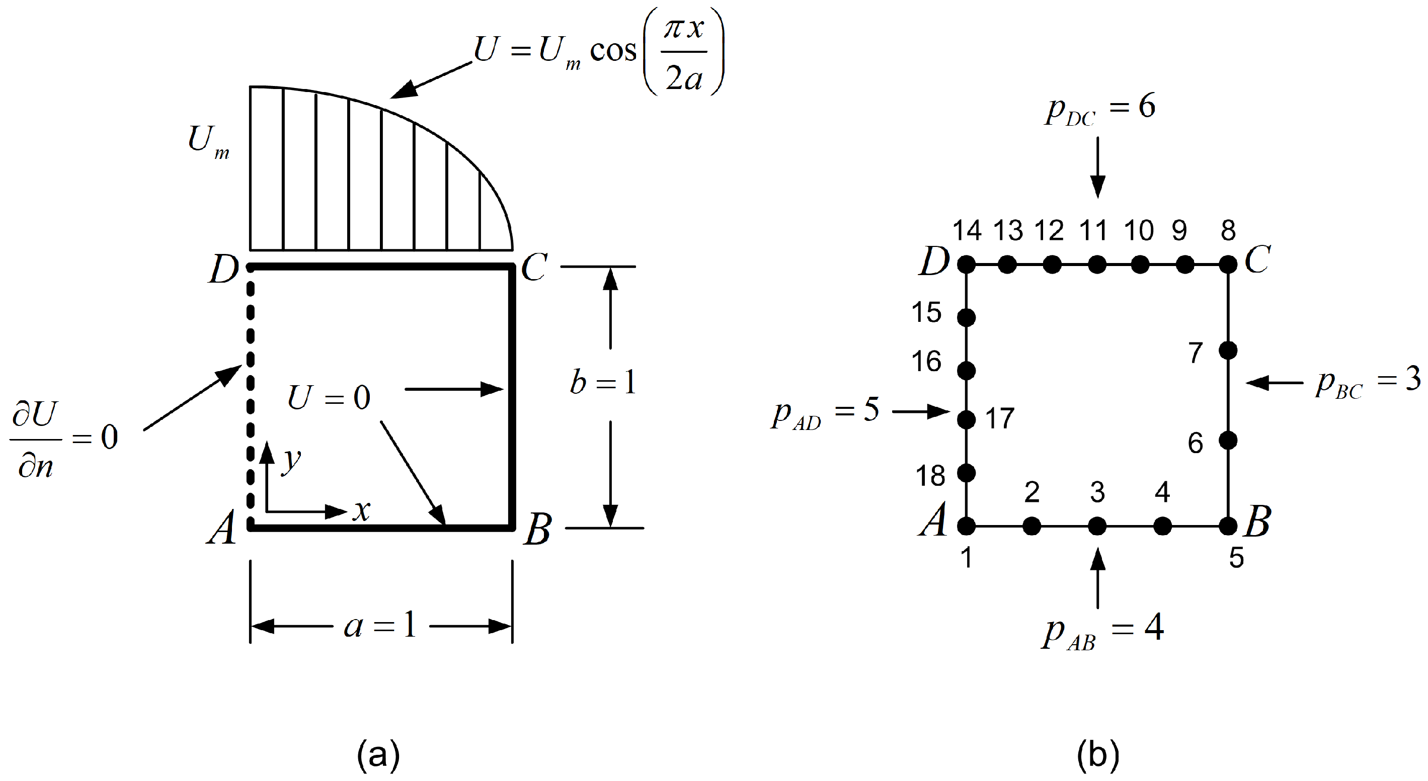
Let us consider a square domain of dimensions in which the Laplace equation dominates . The boundary conditions are partially of the Dirichlet and Neumann types, as shown in Figure 2a. The temperature along the top edge is given as
The exact solution is given as:
whereas the error norm is defined (in percent %) as
Solution: The entire patch was discretized as a single tensor product element of 20 degrees of freedom (DOFs) shown in Figure 2b (with polynomial degrees and ), of which only 9 DOFs (i.e., 5, 6, 7, 9, 10, 11, 13, 14, 15) are unrestrained. Using either Lagrange or Bernstein polynomials, the calculated error was found to be the same, equal to . The only difference was the condition number of the equations’ matrix (of size ), which was found to be equal to 41.8 and 55.3 for Lagrange and Bernstein polynomials, respectively.
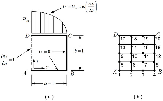
Figure 2.
Square domain: (a) Dimensions and boundary conditions. (b) Tensor product discretization.
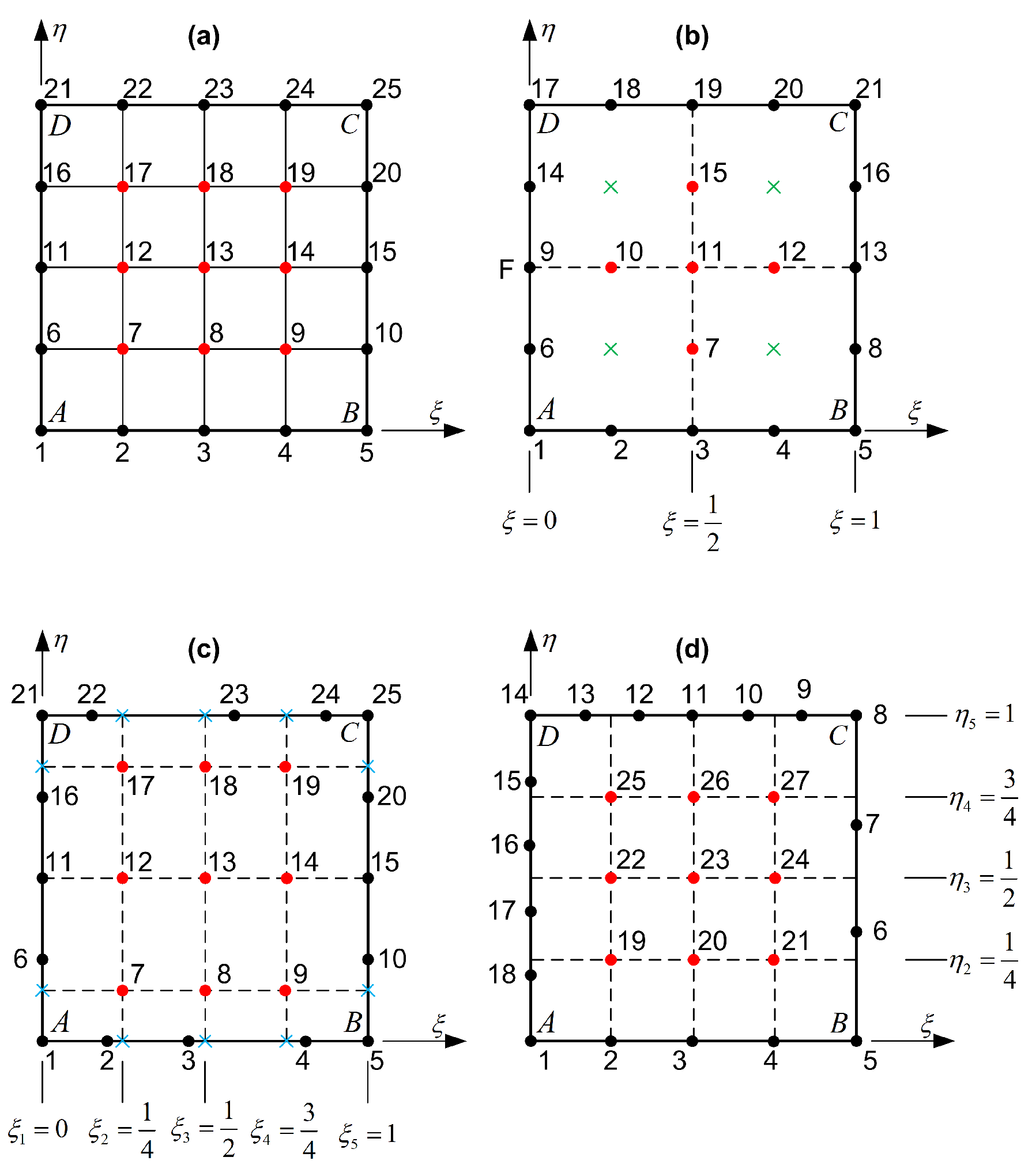
To further investigate the relationship between equivalent polynomials, in the tensor product we used non-uniform Lagrange polynomials toward the y-direction, with nodal points at (or (i.e., slightly refined close to the top edge ). It was found that, using non-uniform Lagrange polynomials, the -norm was insensitive. In contrast, the condition number was sensitive, since it varied between 37.7 and 53.2 for the ordinate of the nodal point 13 below the corner D shown in Figure 2b, with and , respectively. Despite the non-uniform location of nodal points in the y-direction, the linear mapping was preserved (i.e., ) and (closely related) the determinant of the Jacobian was always constant, equal to unity. Moreover, in the formulation using Bernstein polynomials, it is critical to preserve the control points at their initial uniform positions to ensure this linear mapping (and not to move them at the non-uniform nodal points of the Lagrange-based model), and then (obviously) the -norm is preserved the same as in the formulation of Lagrange polynomials (since nothing changes); otherwise, the Jacobian becomes variable and the error norm substantially increases.
By comparing the two column vectors in Equation (13), one observes that, in the case of tensor product Bernstein polynomials, it is sufficient to replace the Lagrange polynomials with Bernstein polynomials of the same degree. However, it remains unclear whether this substitution strategy can be extended to other classes of non-tensor product macroelements. One such class includes classical transfinite elements, which, while structurally similar to tensor product elements, lack many of the nodes present in a full tensor product configuration. This case is examined in detail in Section 4.
3.5. Cross-Check
The same result with Equation (15) can be obtained performing the operations in Equation (6). For the nine-node element with node numbering according to Figure 1b, each of the transformation matrices is equal to the matrix shown on the right-hand side of Equation (8). The matrices and include the following entries:
The interested reader may also consult a MATLAB R2014b script given in Appendix A, which performs the comparison between the matrix (of size ) with the column-vector (of size ), which is calculated through Equation (15) and is defined as
4. Classical Transfinite Elements
Classical transfinite elements cover the entire or a large portion of a parametric quadrilateral patch . They consist of nodes ordered along horizontal and vertical stations (cuts or sections) that are perpendicular to the and parametric axes and are very similar to the 21-node element shown in Figure 3. Traditionally, the transfinite elements are characterized by the following two functional sets:
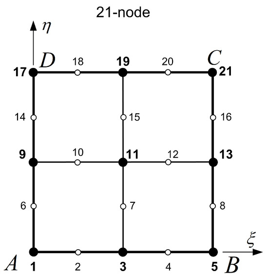
Figure 3.
The classical 21-node transfinite element.
- Blending functions. For each direction ( or ), the number of blending functions equals the number of corresponding stations, and thus their polynomial degree ( or , accordingly) equals . For example, in the 21-node element shown in Figure 3, there are three stations per direction and thus . Perpendicularly to the -direction (toward -axis), the first vertical station is the edge (with nodes 1-6-9-14-17), the second vertical station consists of the nodes (3-7-11-15-19), and the third one includes the nodes along edge (with nodes 5-8-13-16-21). Similarly, perpendicularly to the -direction (toward -axis), there are also three horizontal stations, i.e., the edge (with nodes 1-to-5), the isoline made of nodes (9-10-11-12-13), and eventually the edge (with nodes 17-to-21).
- Trial functions. These refer to the interpolation along the stations. In this example, each station consists of 5 nodes (4 node spans), and thus the polynomial degree will be (e.g., along the horizontal edge ), and similarly (e.g., along the vertical edge ). In general (for other discretizations), we have .
One may observe that this specific 21-node element may be produced from a tensor product of size (25 nodes), from which 4 nodes (i.e., the centers of the four cells: 1-3-11-9, 3-5-13-11, etc.) are missing. Elements of this type have been extensively studied by their originators [20] as well as by later researchers [19].
At this point, we must point out that the utilization of Lagrange polynomials in transfinite formulation is very clear and reasonable (however heuristic), as follows. The blending functions interpolate the quantity along the horizontal and vertical stations independently (thus forming the projectors and ), and then perform a bivariate correction by subtracting the projector .
While the use of Lagrange polynomials in classical transfinite elements is well established, the same cannot be said for Bernstein polynomials. Thus, although in tensor product elements it is sufficient to replace Lagrange polynomials with Bernstein polynomials of the same degree (see the end of Section 3.4), it remains uncertain whether this substitution is universally valid for classical transfinite elements. Although this approach has been intuitively applied with success in previous work [17], a rigorous theoretical justification has yet to be established.
In this paper, I undertake a detailed investigation into the underlying reasons for the observed numerical agreement in accuracy between Lagrange and Bernstein polynomials, and whether this similarity arises solely from the substitution of polynomials of the same degree.
4.1. General Relationships Between Initial and Transformed Bases
Before going on, it is worth mentioning that for any change of basis there are some standard relationships between the quantities of the two sets. A special discussion on the symmetric eigenvalue problem may be found in [2] (pp. 51–60). In more detail, let be the column-vector of all the shape functions, the vector of the Cartesian coordinates of nodal points, and the nodal displacements (potentials) in the system of Lagrange polynomials. Moreover, in the Bernstein set, the corresponding shape functions are , the control points are , and the coefficients (generalized coordinates) are . Between Lagrange- and Bernstein-based systems, we have the following linear relationships:
For the shape functions, we have
For the degrees of freedom (DOFs), we have
One may observe that the above matrix formulations are consistent with the expressions of the dependent variable in the two systems, as follows:
To determine the control points that define the same parameterization in both systems, we adopt the isoparametric concept (very similar to Equation (35)):
Thus, the analogous expression with Equation (34) for the control points is
4.2. Structured Transfinite Elements
In this subsection, I focus on the classical structured transfinite elements, which are characterized by horizontal and vertical stations that are subdivided by several nodes like the 21-node element shown in Figure 3. The characteristic of this element, and similar ones, is the same number and the same location of nodal points along all stations parallel to one direction, individually. It has been discussed in [17] that, taking into consideration that the blending functions are quadratic Lagrange polynomials (because there are three parallel stations per direction) whereas the trial functions are quintic Lagrange polynomials (because there are five nodes per station), the three projectors of the Boolean sum can be constructed. To shorten their presentation, in this paper I prefer an alternative, which is the following robust matrix formulation:
and
According to the standard theory [20], the transfinite interpolation of the bivariate dependent variable is given, in terms of three projectors, as
Substituting the three projectors, i.e., Equations (38)–(40), into Equation (41), the extraction of coefficients gives the following expression:
where the global bivariate shape functions are given in terms of Lagrange polynomials by
If we return to Equations (38)–(40), we can easily replace the univariate row and column vectors of the Lagrange polynomials ( or ) by the equal products of the transformation matrices ( or ) times the corresponding vector of Bernstein polynomials ( or ) according to Equations (3) and (4). Then, in short notation, Equation (41) becomes
One may observe that the right-hand side of Equation (44) includes three matrices, of which the entries are linear combinations of the values (obviously, they represent generalized coefficients)—i.e.,
Thus, Equation (44) can be written as
From the two equalities of Equation (44), which are very similar, the first in terms of Lagrange polynomials and the second in terms of Bernstein polynomials, one may easily understand that the two sets of Lagrange polynomials in Equation (43), i.e., those of degree and , are replaced by Bernstein polynomials of the same degree, one-by-one. Therefore, the second equality of Equation (44) eventually leads to the expression
where gives the generalized coordinates (DOFs in a Bernstein system). Moreover, the produced functional set is quite equivalent, given by
Interestingly, the three matrices, i.e., (, and ), do not have the structured form of ( and ) shown in Equations (38)–(40), but are influenced by all the coefficients in a rather complicated way. This in turn means that the three projectors do not preserve their form in the two functional systems separately, but the totality in their Boolean sum (Equation (41)) does.
Furthermore, using their actual binomial forms and equating the coefficients of the same monomials in both systems (Lagrange, Bernstein), it can be shown (and is easily verified) that the two functional sets, i.e., and , are linearly interrelated according to Equation (33), where the transformation matrix is given as
4.3. Numerical Verification of 21-Node Traditional Transfinite Element
The 21-node transfinite element is one of the elements studied in the mid-1970s [20]. As previously mentioned, the nodal points are arranged along three stations per direction, in such a way that one node is missing for each of the four cells of this patch, to form the associated ideal tensor product.
We again solve the same problem (Laplace equation) with the same boundary conditions as in Example 1, but now using a single 21-node macroelement (Figure 3). In both formulations (Lagrange, Bernstein), the error norm is found to be . Obviously, this finding is consistent with the existence of the transformation matrix (given by Equation (51)) between these two functional sets, as discussed in Section 4.2.
Important remark: From the above discussion, it becomes obvious that, in tensor products and for classical (structured) transfinite elements, the expressions of the basis functions using Bernstein polynomials are the same with those of shape functions using Lagrange polynomials, where the same degree is considered.
5. Distorted Tensor Products and Partially Unstructured Transfinite Elements
We recall that in the first two classes discussed above—namely, the tensor product elements and the classical structured transfinite elements (Figure 4a,b)—this paper has theoretically demonstrated (see Section 3 and Section 4, respectively) that Lagrange polynomials can be directly replaced by Bernstein polynomials of the same degree, with numerical results remaining unchanged, except for the condition number of the resulting system of equations.
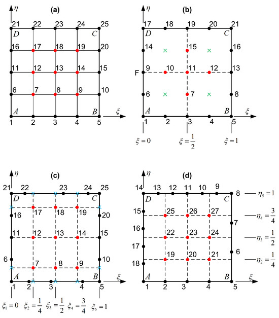
Figure 4.
Basic categories of transfinite elements: (a) tensor product, (b) classical structured, (c) distorted tensor product, and (d) partially unstructured (Red circle: internal node; Blue cross: artificial (auxiliary) node; Green cross: missing node).
In this section, we will examine whether the mutual substitutability between Lagrange and Bernstein polynomials also extends to other transfinite configurations. Among the various alternative configurations of transfinite elements, we will focus here on those in which the internal nodes form a tensor product grid, while the boundary nodes may not adhere to this structure. Two classes of such elements are considered in Section 5.1 and Section 5.2, respectively.
5.1. Simple Distortion
This subsection addresses elements in which the internal nodes are uniformly arranged in a tensor product pattern, while the boundary node positions do not fully align with this structure. Figure 4c illustrates a distorted tensor product 25-node transfinite element, where the internal nodes form a tensor product grid, but their orthogonal projections do not coincide with the boundary nodes. In this configuration, Lagrange polynomials are employed as uniform blending functions, and , of degree 4. In contrast, the trial functions, and , are non-uniform polynomials, also of degree 4. The key distinction between the blending and trial functions—despite both being of degree —lies in their construction: the blending functions are defined over a uniform node distribution, whereas the trial functions correspond to a generally non-uniform nodal sequence along the four edges.
5.1.1. Closed-Form Expressions
Despite the geometric distortion of the element illustrated in Figure 4c, transfinite interpolation remains applicable. Its implementation, however, necessitates the introduction of auxiliary (artificial) nodes, which are subsequently eliminated—a procedure also detailed in Section 5.2.1. Accordingly, the analogue of Equation (43), formulated using transfinite interpolation based solely on Lagrange polynomials, results in the following set of basis functions. For brevity, we present here only the functions associated with the bottom edge :
In Equation (52), the superscripts () and () were set to denote the edges along which the non-uniform Lagrange polynomials operate. Clearly, Lagrange polynomials require uniform (evenly) and non-uniform (non equally spaced) sets of nodal points.
The application of Bernstein polynomials to the same geometrically distorted element (Figure 4c) is not immediately straightforward. This is primarily because, except for the four boundary edges of the patch, interpolation along any internal isoline generally depends on all the coefficients a; that is, it is influenced by more than just the degrees of freedom (or nodal coordinates) located along the isoline under consideration. In contrast, the cardinal property of Lagrange polynomials enables the use of artificial nodes to achieve local interpolation along each station, as discussed previously.
Nevertheless, it has been conjectured in Ref. [18] that Bernstein polynomials can effectively serve as both blending and trial functions. Accordingly, the (uniform or non-uniform) Lagrange polynomials employed in Equation (50) can be substituted with Bernstein polynomials of the same degree. The corresponding analogue of Equation (50) is then given by
A careful inspection of Equation (53) reveals that, after simplification, the bivariate basis functions associated with the element depicted in Figure 4c reduce to the tensor products of univariate Bernstein polynomials. In other words, for distorted tensor product patches, the shape functions derived from Lagrange polynomials inherently depend on the spatial distribution of the nodal points, whereas the basis functions formed from Bernstein polynomials remain fixed and independent of geometry (see Figure 5). Consequently, in the Bernstein formulation, geometric distortion is fully absorbed by the generalized coefficients .

Figure 5.
Twenty-five-node distorted tensor product element.
Moreover, to reproduce results equivalent to those obtained using Lagrange polynomials, it is necessary to assign the control points specific positions that do not coincide with the Cartesian coordinates of the nodal points. Instead, these control points are related to the nodal positions via the following well-known transformation:
By collocating Equation (54) at the 25 nodal points associated with the Lagrange set, the nodal coordinates appear on the left-hand side, while the right-hand side contains the unknown control points . This leads to a linear system of 25 equations with 25 unknowns, which can be solved to determine the positions of the control points.
5.1.2. Numerical Verification
It is worth noting that, when Example 1 was solved using both functional sets for the 25-node element, the resulting error norm was identically . This same error was observed even when the positions of the nodes along three edges (, , and ) were varied. A slight variation in the error was detected only when modifying the positions of the three intermediate nodes along the top edge , where non-homogeneous Dirichlet boundary conditions are imposed. For instance, after assigning the Cartesian coordinates , and in the Lagrange-based model (and applying the corresponding modifications in the Bernstein-based model), the error increased marginally to in both cases. These results are consistent with expectations, since the two functional systems are inherently connected via the transformation matrix , as defined in Equation (14).
5.2. Distortion Combined with Node Refinement or Removal on Edges
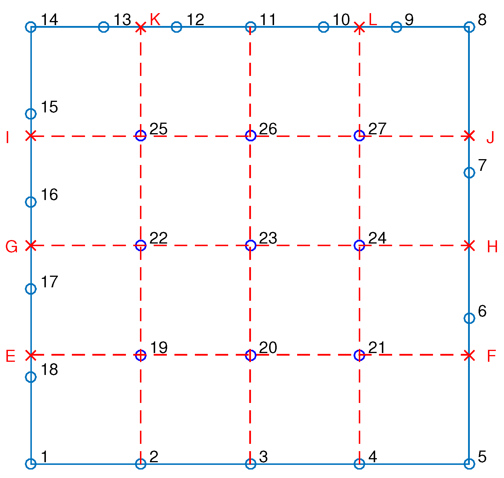
In the previous Section 5.1, we examined a simple geometric distortion of the patch , where the boundary nodes were displaced from their original positions and associated with an ideal tensor product structure. In this section, we consider a similar type of distortion, but additionally allow for variations in the number of nodes along one or more edges. For instance, as illustrated in Figure 4d, the edge remains unaltered (degree ), one node has been removed from edge (degree ), two nodes have been added to edge (degree ), and one node has been added to edge (degree ). As a result, the original 25-node configuration described in Section 5.1 is transformed into a 27-node transfinite element comprising 18 boundary nodes () and 9 internal nodes.
In the set of Lagrange polynomials, the shape functions have the form of those involved in Equation (43):
- Shape functions associated with corner nodes consist of three terms (influenced by all the three projectors, and ).
- Shape functions associated with intermediate nodes on the edges consist of one term, which is related to the projector having as a subscript the axis perpendicular to the current edge. For example, the shape functions of nodes along edge are influenced by only the projector .
- Shape functions associated with internal nodes equal to the tensor product of the blending functions only.
Typical expressions, one for each category, are given in Equation (55) below:
Although a rigorous mathematical foundation has not yet been established, previous numerical evidence supports a reasonable choice: replacing the fourth-degree Lagrange polynomials used as blending functions with Bernstein polynomials of the same degree, that is,
where s represents either of the parameters or . Similarly, the trial functions along the edges to , which are Lagrange polynomials of degree 4, 3, 6, and 5, respectively, are substituted by Bernstein polynomials of the same degree, as shown in Equation (57) below:
In both cases, the shape functions (bivariate Lagrange) and basis functions (bivariate Bernstein) fulfil the partition of unity (rigid-body) and the constant strain property, as shown in Equation (58) below:
Moreover, in both cases the determinant of the Jacobian is equal to unity (det), which implies that the mapping from the parametric space to the physical space is affine (or identity-like in behavior) over a square.
With respect to the aforementioned 27-node transfinite element, a previous study on the interpolation of a bivariate function revealed a minor discrepancy between the use of Lagrange and Bernstein polynomials (see [18], p. 22). In the following, this difference is further examined and justified, and corresponding numerical results are presented for the solution of Example 1 (defined in Section 3.4).
5.2.1. Justification
An explanation for the above discrepancy is provided as follows. When using Lagrange polynomials, which are directly associated with the nodal values , the interpolation mechanism employed is transfinite interpolation [20]. Within this framework, the blending functions are used to interpolate the function along isolines that are perpendicular to the -axis at positions ; this process corresponds to the projector . Similarly, the blending functions interpolate the function along isolines perpendicular to the -axis at positions , which defines the projector . To avoid redundancy in the combined interpolation , a corrective term is introduced. The final interpolated expression follows the Boolean sum formulation, as expressed in Equation (41), namely, .
In the example of the 27-node transfinite element—shown in greater detail in Figure 6—a notable characteristic is that the orthogonal projections of certain internal nodes onto the patch edges do not coincide with existing boundary nodes. In fact, all internal nodes exhibit this misalignment in at least one parametric direction. To address this issue, artificial nodes (denoted as ) are introduced to complete the missing starting and/or ending nodal points required for the definition of the relevant Lagrange polynomial sequences on the internal stations. This enables the proper formulation of the functions and , which are essential for applying transfinite interpolation.
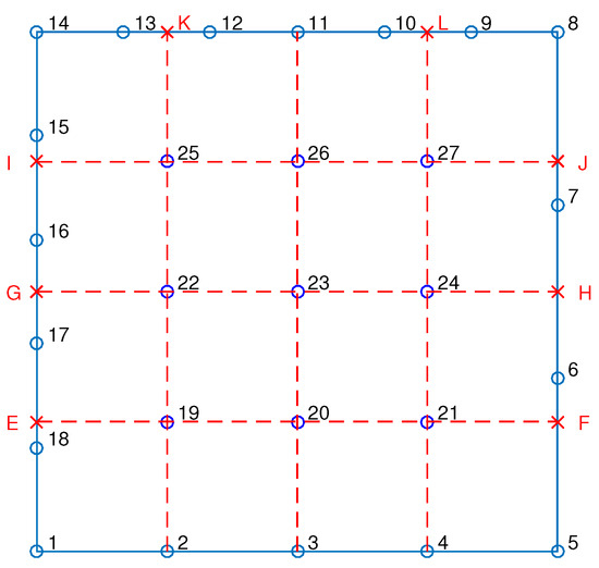
Figure 6.
The 27-node transfinite element.
We recall that the corrective projector includes all the () intersections between 5 stations per direction, and thus may be written in terms of primary and artificial (red-colored) nodes as
Obviously, each vector including blending functions (Lagrange polynomials of degree 5) can be substituted by Bernstein polynomials of degree 5 as well, where
with
This in turn means that the projector preserves its form after transformation (from Lagrange to Bernstein polynomial), which then becomes
On the other hand, the projector includes some of the primary nodes (1 to 27) and some of the artificial nodes. In more detail,
- The function consists of six nodal values , which define 5 node spans and fully define a polynomial of degree 5. Note that the artificial nodes are not included because they are not needed.
- The function consists of 5 nodal values (4 node spans), and thus fully defines a polynomial of degree 4. Note that the artificial node K, on the boundary, is required to determine the missing end of nodal sequence.
- The function consists of 5 nodal values (4 node spans), and thus fully defines a polynomial of degree 4. All entries of the nodal sequence are primary nodes that belong to the 27-node element.
- The function consists of 5 nodal values (4 node spans), and thus fully defines a polynomial of degree 4. Note that the artificial node L is required to determine the missing end of the nodal sequence.
- The function consists of four nodal values , defining 3 node spans and fully defining a polynomial of degree 3. Note that the artificial nodes , on the boundary, are not included because they are not needed.
The above-mentioned different number of nodes along the isolines at does not allow for as elegant a mathematical form as that in Equation (59). This means that a row vector of the Lagrange polynomials in cannot be extracted as a common factor, and that the next matrix of the nodal values is not fully populated. Therefore, we write in a conventional manner as follows:
One may observe in Equation (63) that only two out of the eight artificial nodes () are included in .
Similar observations may be made for projector , which can be written as follows:
One may observe in Equation (64) that six out of the eight artificial nodes () are included in .
In summary,
- The projector includes two out of the eight artificial nodal values.
- The projector includes the rest six out of the eight artificial nodal values.
- The subtractive corrective projector includes all the eight artificial nodes.
Interestingly, for every chosen artificial nodal value, for example, for , the unique associated term in is cancelled by the corresponding opposite term cited in . Ultimately, one may verify that two terms of and six terms of , which include artficial DOFs, are cancelled by the corresponding eight terms in , and thus are eventually eliminated. As a result, the Boolean sum will contain only the 27 primary DOFs that define the 27-node transfinite element. In more detail, the terms related to the eight auxiliary (artificial) points vanish, as follows:
- We notice the terms , coming from and .
- We notice the terms , coming from and .
- We notice the terms , coming from and .
- We notice the terms , coming from and .
- We notice the terms , coming from and .
- We notice the terms , coming from and .
- We notice the terms , coming from and .
- We notice the terms , coming from and .
Substituting Equations (59), (63), and (64) into the Boolean sum , for the Lagrange-based system, the latter gives the following shape functions (see also Figure 7a):
Interestingly, the shape functions and , although being associated with corner nodes, consist of only one term (i.e., eventually influenced by only the projector ), because the trial functions along their common edge are exactly equal to the corresponding blending functions (uniform of degree 4).

Figure 7.
Shape and basis functions of 27-node transfinite element.
We recall that the origin of transfinite interpolation is heuristic, and thus any extension of it will be heuristic as well. In this context, by intuition, one could conjecture that transfinite interpolation is also applicable using Bernstein polynomials in the position of blending and trial functions as well. Then, Equation (65) would take the following form (see Figure 7b):
It can be verified that both sets of shape and basis functions, respectively, fulfil the partition of unity property:
Nevertheless, there is no guarantee that these two bases are completely equivalent (see Section 5.2.2). One may observe that due to the non-symmetric form of the terms involved in Equations (63) and (64), the direct substitution of Lagrange by Bernstein polynomials does not achieve the same expression exactly. In more detail, each of the row vectors in Equation (63) can be replaced by a matrix equation like that of Equation (60). For degree , we have the transformation matrix given by Equation (61), whereas for degrees 3, 4, and 6, we have
Applying the transformation matrix (see Equation (69)) to the Bernstein-based basis functions through along edge yields an accurate reconstruction of the corresponding Lagrange-based shape functions through . Similar results are observed for the remaining three edges as well.
One would anticipate that replacing all Lagrange polynomials involved in the three projectors (Equations (59), (63), and (64)) through transformation matrices would lead to an expression of the bivariate function in terms of Berntein polynomials. Nevertheless, such an approach would lead to a high number of products in the form . A rough estimation gives 180 terms while we need only 27, plus a few more for the basis functions and associated with the corners. Theoretically, such a functional set probably exists, but the paper at hand has not achieved to tackle this topic, which still remains open. Some initial observations may be useful for future research:
- The transformation matrix , which fulfils the relationship , is determined by applying it to all the 27 nodal points of the element; we receive that det .
- The recalculation of the Lagrange-based bivariate shape functions in terms of the Bernstein-based ones , using the relation , shows a large error (about ) in the interior of the element, whereas on the boundary and at the nodal points it vanishes.
- A similar discrepancy was observed when the relationship was applied to more points, and this least-squares scheme led again to a similar deviation between the initial and the recalculated values.
5.2.2. Numerical Verification
The same BVP was solved using the 27-node transfinite element, with uniform discretization per edge, in conjunction with both formulations. The results are as follows:
- The requirement to use the parameters defined by the nodal points of the Lagrange model, and then map the control points to the nodal points , leads to coincidence between them.
- In both systems, the determinant of the Jacobian all over the rectangular domain is equal to unity.
- The error norm was found to be slightly different in each system: for the Lagrange polynomials and for the Bernstein ones.
Although the Bernstein basis is known for its robustness, the observed discrepancy between the Lagrange and Bernstein polynomial systems indicates that a straightforward substitution of Lagrange polynomials with Bernstein polynomials may not be optimal for this class of transfinite elements. A more comprehensive theoretical analysis is necessary to fully elucidate this behavior, akin to the discussions presented in Section 4.2.
6. Coons Interpolation
The Coons interpolation [21] is probably the oldest interpolaton formula in computer-aided geometric design (CAGD) (for example, see [22]), which later inspired the transfinite interpolation [20]. It refers to a quadrilateral patch , of which the four edges are of given geometry or of given function U. Given the linear blending functions (), and the four univariate functions associated with the four edges, at each pair the variable U is interpolated by
Now, we will test whether Lagrange polynomials in Equation (71) may be substituted with Bernstein polynomials while the result remains the same. It is trivial to notice that linear Bernstein polynomials are identical to linear Lagrange polynomials, and therefore there is no question about the replacement of and with and , respectively. Moreover, since each edge is equivalently described by either a set of Lagrange polynomials or a set of (non-rational) Bernstein polynomials, because both sets are unitary (take unit value) at the corners, it is obvious that the four univariate functions , and may be equivalently represented in these two ways. Consequently, we have proven that all terms in the Coons interpolation formula described by Equation (71) can be represented either in terms of Lagrange or in terms of Bernstein polynomials. In other words, every expression—such as the set of shape functions—derived from Coons’ interpolation and expressed using Lagrange polynomials can also be expressed in terms of Bernstein polynomials by merely replacing the Lagrange polynomials, one-by-one, with a Berstein polynomial of the same degree.
Typical shape functions in terms of Lagrange polynomials are given below:
where and are the polynomial degrees along the edges and , respectively.
Moreover, typical basis functions in terms of Bernstein polynomials are given below:
6.1. Numerical Verification
The same BVP (Example 1: Laplace equation in square domain) was solved for a single Coons element made of 18 DOFs, as shown in Figure 8b (note that this Coons element is the same as the 27-node element shown in Figure 4d, but without the 9 internal nodes). This was chosen to cover one of the most general cases, because the polynomial degrees in the trial functions along the four edges are equal to 4, 3, 6, and 5, respectively. Using either of the polynomial sets, i.e., Lagrange or Bernstein, the error norm was found equal to 2.3013%.
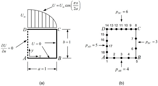
Figure 8.
(a) Geometry and boundary conditions. (b) Discretization.
Working in a similar way as in Section 4.2, the transformation matrix () between the Lagrange and Bernstein basis (see Equation (33)) for the 18-node Coons element is as follows:
7. Numerical Solution of Eigenvalue Problem
In addition to the Laplace equation, which served as the first example in the preceding sections of this paper, this section introduces a second problem, as detailed below.
Example 2.
Eigenvalue analysis of rectangle acoustic cavity.
A rectangular acoustic cavity of dimensions and normalized wave velocity c = 1 m/s is under Neumann boundary conditions (), representing hard walls (i.e., full reflection). The exact solution is given as follows (see [23]):
For each eigenvalue, the error (in %) is calculated using the following formula:
This problem was solved using the following four models:
Using either Lagrange polynomials or Bernstein polynomials, for the above first three models (18-node and 25-node elements), for all natural modes, the results are the same, as selectively shown in Table 1.

Table 1.
Calculated eigenvalues (errors in %).
Moreover, for the 27-node element, the results differ, as shown in Table 2. One may observe that now the two models (Lagrange and Bernstein) do not coincide, but the quality of the results is similar, if not slightly better for the Bernstein-based element.
Table 2.
Calculated eigenvalues (errors in %) for the 27-node transfinite element.
8. Discussion
In this paper, five classes of transfinite elements were investigated, as described in the Introduction section (Section 1). Below, I summarize the findings for each of them.
Coons Element. The simplest transfinite element is the Coons element, which consists of boundary nodes only. This element was theoretically explained, and it was numerically verified that if either Lagrange or Bernstein polynomials are implemented in the Coons interpolation formula, the result in the numerical solution of a PDE is the same (see Section 6.1). Moreover, for an 18-node Coons element, the transformation matrix between the Lagrange-based and Bernstein-based bivariate shape functions was determined.
Tensor Product Element. It is well known that tensor product Lagrange polynomials are equivalent to non-rational tensor product Bernstein polynomials (see [19], among others). In the present paper, it was demonstrated that an inherent transformation matrix exists between these two bivariate functional sets, which can be systematically constructed from two one-dimensional constituent transformation matrices—one for each parametric direction.
Classical Transfinite Element (Structured). It was also shown, by numerical examples, that classical transfinite elements with structured horizontal and vertical stations (such that of 21-node shown in Figure 3) can be equally treated substituting both the blending and trial functions one-by-one, from Lagrange polynomials to Bernstein polynomials of the same degree [17]. The present paper showed that when mathematically replacing univariate Lagrange polynomials with univariate Bernstein polynomials within the transfinite interpolation formula, we receive the same expression, the only difference being that the Lagrange-based bivariate shape functions are substituted with Bernstein-based bivariate basis functions. Moreover, the nature of the associated generalized coefficients (in terms of nodal values ) was revealed. Finally, the inherent transformation matrix between the two bivariate sets of shape and basis functions was explicitely determined (see Equation (51)).
Distorted Tensor Product Element. It is known that even elements in which the boundary nodes do not match the orthogonal projections of internal nodes onto edges can be treated using the transfinite interpolation formula [20]. This issue has been reported since at least 1995 (see details in [19]) by introducing ‘artificial’ nodes that eventually disappear. In brief, the shape functions associated with the interior of edges and the interior of the domain are local tensor products of blending and trial functions, whereas those associated with the four corners of the patch are influenced by all of the three projectors . The paper at hand shows that the same numerical result with the aforementioned ‘distorted’ transfinite element based on Lagrange polynomials is also obtained when using tensor product Bernstein polynomials with properly chosen control points. The required condition is that the ‘images’ of the control points (see Equation (37)) must be exactly that of the distorted element nodes in the Lagrange-based formulation.
Partially Unstructured Element. Beyond the aforementioned simple distortion of tensor product elements with respect to node placement, there exists a case where a given edge of the patch contains a different number of nodal points than its opposite (and parallel, in the parametric space) edge. For instance, the 27-node element depicted in Figure 4d (as well as in Figure 6) can be treated as a transfinite element, similarly to the previously discussed 25-node distorted configuration. However, when Bernstein polynomials are directly substituted for Lagrange polynomials of the same degree, a prior study reported only a slight difference in average interpolation error—specifically, 0.6408% for the Lagrange system versus 0.6154% for the Bernstein system—when interpolating the bivariate function ([18], p. 22). To further investigate this discrepancy, the present work revisits the topic within the framework of a boundary-value problem (BVP), where a similar trend was observed: the error norm of the numerical solution differed only slightly (0.0191% for Lagrange vs. 0.0126% for Bernstein), as shown in Section 5.2.1. It was also found that a standard transformation matrix between Lagrange and Bernstein basis functions does not exist in a general sense, as it depends on the specific test points at which the two bases are related. A second example, presented in Section 7, confirmed a comparable behavior. Interestingly, in all three test cases, the Bernstein-based model marginally outperformed the corresponding Lagrange-based formulation.
In summary, the findings of this study indicate the following:
- For four broad classes—namely, (i) Coons elements, (ii) tensor product elements, (iii) classical transfinite elements with a structured pattern of internal nodes, and (iv) distorted tensor product elements—Bernstein polynomials can directly replace Lagrange polynomials of the same degree, yielding identical accuracy.
- In a fifth class, involving transfinite elements with arbitrary boundary nodes and a tensor product distribution of internal nodes, Bernstein polynomials may also be used in place of Lagrange polynomials of the same degree. However, this substitution does not guarantee identical results. While the overall performance of such arbitrarily noded transfinite elements remains satisfactory for practical applications, further investigation is needed, especially in cases involving non-uniform polynomial degrees.
9. Conclusions
This study demonstrates that transfinite finite elements can be effectively combined with Bernstein–Bézier polynomials by substituting Lagrange polynomials with their Bernstein counterparts. This substitution preserves the partition of unity across all five examined element classes: Coons-based elements, tensor product elements, structured-node transfinite elements, distorted tensor product elements, and elements with arbitrarily placed nodes and varying polynomial degrees along opposing edges. While the first four classes achieve accuracy equivalent to that of the original Lagrange-based formulation, the fifth class exhibits minor discrepancies. Although the Bernstein-based approach remains computationally robust and practically effective in this most general case, the question of full mathematical equivalence in terms of accuracy remains open and warrants further investigation.
Funding
This research received no external funding.
Institutional Review Board Statement
Not applicable.
Informed Consent Statement
Not applicable.
Data Availability Statement
Data are available upon request.
Conflicts of Interest
The author declares no conflicts of interest.
Appendix A. MATLAB Script for Matrix Comparison
The MATLAB code used for calculating the matrix comparison is given in Listing A1.
This code symbolically deals with the nine entries of matrix . In the beginning, the 1D transformation matrix is explicitly given. The variable Aexact1 represents the exact multiplication (cf. Equation (6)), the variable R represents Equation (15), and the former matrix is reconstructed into the vector Areconstructed. Moreover, the vector Aexact2 represents the product , where is the same as matrix (of size ) but written as a column vector of size (cf. Equation (32)). At the end, the code verifies that the reconstructed vector of generalized coefficients Areconstructed is the same as Aexact2.
| Listing A1. Auxiliary MATLAB code to experiment with the matrix as a matrix of size 3 × 3 or as a column-vector of size 9 × 1, for quadratic interpolation (p = 2). |
| clear all |
| clc |
| syms U1 U2 U3 U4 U5 U6 U7 U8 U9 |
| syms A1 A2 A3 A4 A5 A6 A7 A8 A9 |
| syms R |
| Tx = [ 1 −1/2 0 |
| 0 2 0 |
| 0 −1/2 1]; |
| Ty = Tx; |
| U = [U1 U4 U7 |
| U2 U5 U8 |
| U3 U6 U9]; |
| Aexact1 = Tx’ ∗ U ∗ Ty |
| Areconstructed = Aexact1 (:); |
| R = [… |
| 1 −1/2 0 −1/2 1/4 0 0 0 0 |
| 0 2 0 0 −1 0 0 0 0 |
| 0 −1/2 1 0 1/4 −1/2 0 0 0 |
| 0 0 0 2 −1 0 0 0 0 |
| 0 0 0 0 4 0 0 0 0 |
| 0 0 0 0 −1 2 0 0 0 |
| 0 0 0 −1/2 1/4 0 1 −1/2 0 |
| 0 0 0 0 −1 0 0 2 0 |
| 0 0 0 0 1/4 −1/2 0 −1/2 1 ]; |
| Uvector = transpose([U1 U2 U3 U4 U5 U6 U7 U8 U9]); |
| Aexact2 = R.’ ∗ Uvector |
| isEqual = isequal(Areconstructed, Aexact2); |
| if isEqual |
| disp(’The symbolic matrix and vector storage are equivalent.’); |
| else |
| disp(’The symbolic matrix and vector storage are NOT equivalent.’); |
| end |
References
- Zienkiewicz, O.C. The Finite Element Method, 3rd ed.; McGraw-Hill: London, UK, 1977. [Google Scholar]
- Bathe, K.J. Finite Element Procedures, 2nd ed.; Prentice-Hall: Hoboken, NJ, USA, 1996. [Google Scholar]
- Cottrell, J.A.; Hughes, T.J.R.; Bazilevs, Y. Isogeometric Analysis: Towards Integration of CAD and FEA, 1st ed.; Wiley: Chichester, NH, USA, 2009. [Google Scholar]
- Bernstein, S. Sur une modification de la formule d’interpolation de Lagrange (French, Russian abstract). Commun. Soc. Math. Kharkov 1932, 5, 49–56. [Google Scholar]
- Lorentz, G.G. Bernstein Polynomials, 2nd ed.; Chelsea Publishing Co.: New York, NY, USA, 1986. [Google Scholar]
- Amato, U.; Della Vecchia, B. Bridging Bernstein and Lagrange polynomials. Math. Commun. 2015, 20, 151–160. [Google Scholar]
- Cooper, S.; Waldron, S. The eigenstructure of the Bernstein operator. J. Approx. Theory 2000, 105, 133–165. [Google Scholar] [CrossRef]
- Occorsio, D.; Simoncelli, A.C. How to go from Bézier to Lagrange curves by means of generalized Bézier curves. Facta Univ. Ser. Math. Inform. (Nisˇ) 1996, 11, 101–111. [Google Scholar]
- Micchelli, C. The saturation class and iterates of Bernstein polynomials. J. Approx. Th. 1973, 8, 1–18. [Google Scholar] [CrossRef]
- Tachev, G. From Bernstein polynomials to Lagrange interpolation. In Proceedings of the 2nd International Conference on Modelling and Development of Intelligent Systems (MDIS 2011), Sibiu, Romania, 29 September–2 October 2011; pp. 192–197. [Google Scholar]
- Milovanović, G.V.; Udovičić, Z. Calculation of coefficients of a cardinal B-spline. Appl. Math. Lett. 2010, 23, 1346–1350. [Google Scholar] [CrossRef]
- Dyn, N.; Levin, D. Subdivision schemes in geometric modelling. Acta Numer. 2002, 11, 73–144. [Google Scholar] [CrossRef]
- Kočić, L.M.; Milovanović, G.V. Shape preserving approximations by polynomials and splines. Comput. Math. Appl. 1997, 33, 59–97. [Google Scholar] [CrossRef]
- Gautschi, W.; Milovanović, G.V. Spline approximations to spherically symmetric distributions. Numer. Math. 1986, 49, 111–121. [Google Scholar] [CrossRef]
- Frontini, M.; Gautschi, W.; Milovanović, G.V. Moment-Preserving Spline Approximation on Finite Intervals. Numer. Math. 1987, 50, 503–518. [Google Scholar] [CrossRef]
- Bustamante, J. Bernstein Operators and Their Properties; Springer: Cham, Switzerland, 2017. [Google Scholar]
- Provatidis, C.G. Non-rational and rational transfinite interpolation using Bernstein polynomials. Int. J. Comput. Geom. Appl. 2022, 32, 55–89. [Google Scholar] [CrossRef]
- Provatidis, C. Transfinite patches for isogeometric analysis. Mathematics 2025, 13, 35. [Google Scholar] [CrossRef]
- Provatidis, C.G. Precursors of Isogeometric Analysis: Finite Elements, Boundary Elements, and Collocation Methods; Springer: Cham, Switzerland, 2019. [Google Scholar]
- Gordon, W.J.; Hall, C.A. Transfinite element methods: Blending-function interpolation over arbitrary curved element domains. Numer. Math. 1973, 21, 109–129. [Google Scholar] [CrossRef]
- Coons, S.A. Surfaces for Computer-Aided Design of Space Forms; MIT: Cambridge, MA, USA, 1967. [Google Scholar]
- Farin, G. Curves and Surfaces for CAGD; Morgan Kaufmann-Elsevier: San Francisco, CA, USA, 2022. [Google Scholar] [CrossRef]
- Courant, R.; Hilbert, D. Methods of Mathematical Physics, 1st ed.; InterScience: New York, NY, USA, 1966; Volume I. [Google Scholar]

Disclaimer/Publisher’s Note: The statements, opinions and data contained in all publications are solely those of the individual author(s) and contributor(s) and not of MDPI and/or the editor(s). MDPI and/or the editor(s) disclaim responsibility for any injury to people or property resulting from any ideas, methods, instructions or products referred to in the content. |
© 2025 by the author. Licensee MDPI, Basel, Switzerland. This article is an open access article distributed under the terms and conditions of the Creative Commons Attribution (CC BY) license (https://creativecommons.org/licenses/by/4.0/).