Stability Analysis of SEIAR Model with Age Structure Under Media Effect

Abstract

In this paper, we establish an age-structured SEIAR epidemic model that incorporates media effects and employ the exponential function approach to demonstrate the crucial role of media influence in disease prevention and control. Notably, our model accounts for the possibility of recessive infected individuals becoming dominant through contact with infectious individuals. Theoretical analysis yields the explicit expression for the basic reproduction number $R_0$, which serves as a critical threshold for disease dynamics. Through comprehensive threshold analysis, we investigate the existence and stability of both disease-free and endemic equilibrium states. By applying characteristic equation analysis and the method of characteristics, we establish the following: (1) when $R_0<1$, the disease-free equilibrium is globally asymptotically stable; (2) when $R_0>1$, a unique endemic equilibrium exists and maintains local asymptotic stability under specific conditions. This study shows that strengthening media promotion, raising awareness, and reducing the density of recessive infected individuals can effectively control the further spread of a disease. To validate our theoretical results, we present numerical simulations that quantitatively assess the impact of varying media reporting intensities on epidemic containment measures. These simulations provide practical insights for public health intervention strategies.

1. Introduction

Infectious diseases have always been a major threat to human health. Throughout history, epidemics have posed a serious threat to human survival and nations’ economies. Currently, there are four main research methods for infectious diseases: descriptive research, analytical research, experimental research, and theoretical research [1]. Regarding theoretical research, it is useful to establish mathematical models to describe infectious diseases. The earliest mathematical models designed to describe infectious diseases were established by Kermack and McKendrick [2], and their compartment model, the susceptible–infected–removed (SIR) model, has been widely used and developed. However, for diseases with latent periods of infection and asymptomatic transmission (such as SARS, COVID-19, and foot-and-mouth disease), the susceptible–exposed–infectious–asymptomatic–removed (SEIAR) model is more in line with reality; see [3,4,5,6,7,8] and the references therein for details.

With the rapid development of the internet, people’s access to information is becoming broader and faster. It is well known that media coverage reduces the prevalence of infectious diseases and shortens the duration of infection [9]. The influence of media coverage on diseases is mainly reflected during the initial stages of outbreaks, in which people learn about information related to the disease (transmission principles, routes, and prevention or treatment measures) through media coverage and strengthen their own protection and treatment. Additionally, through official media reports and health education, people’s safety awareness is raised, which may, to some extent, reduce the contact rate between people, as seen with the SARS outbreak of 2002. Regarding research from recent years, Kar and Nandi et al. [10] introduced the media effect through the parameter M, and then Xing and Gao et al. [11], based on the characteristics of media coverage with information implementation rate and reporting lossless rate, expressed the effective contact rate of the disease affected by media coverage as ${\displaystyle \frac{\beta f\left(s\right)I}{1+kM}}$, where M is a constant.

For diseases related to age (such as measles, pertussis, mumps, and COVID-19), considering age factors is more realistic. Age structure is divided into physiological age structure and quasi-age structure, where physiological age is the age that changes over time, and quasi-age refers to age calculated from the day of illness or vaccination. Since the 1970s, many scholars have noted the significant impact of physiological age structure on disease transmission and have established many infectious disease models with age structure to investigate the dynamic behavior for certain infectious models; see [12,13,14,15,16,17,18,19,20,21,22,23] and the references therein.

Based on the above analysis, we will establish a physiological age SEIAR infectious disease model that considers the media effect and uses the exponential function method to demonstrate the impact of media effects on disease transmission. It is assumed that individuals who successfully receive vaccinations will not fall ill again due to immunity and that the natural death rate, vaccination rate, infection rate, and recovery rate are all related to age. Firstly, the existence of both disease-free and endemic equilibrium states is discussed; then, the stability of both disease-free and endemic equilibrium states is studied. Finally, we present numerical simulations to validate our theoretical results.

2. Model Description

We assume that the population can be classified into five different groups, that is, susceptible, exposed, infectious, asymptomatic, and recovered, respectively. $S(a,t)$, $E(a,t)$, $I(a,t)$, $A(a,t)$, and $R(a,t)$ represent the densities of susceptible, exposed, infectious, asymptomatic, and recovered individuals at time t with age a, respectively. The total population is denoted by $N(a,t)$ and the maximum age of an individual by $a^{+}$.

It is noted that exposed individuals can become symptomatic infectives with a probability of p and asymptomatic infectives with a probability of $1-p$ through contact with symptomatic or asymptomatic infectives. Clinical manifestations indicate that asymptomatic individuals cannot become symptomatic infectives through their own toxins, while asymptomatically infected individuals can become symptomatic infectives through contact with infectious individuals with an infectivity rate of $\sigma \left(a\right)$ [14].

In the initial stages of outbreaks, media coverage can reduce the spread of the disease [21]. Therefore, this paper uses an exponential function method to demonstrate the role of media effects in epidemic prevention and control. The exposure rate $\beta (a,b)$ is defined as ${\displaystyle \frac{l\left(a\right)\tilde{\beta }\left(b\right)}{1+h{e}^{j+m\left(a\right)q\left(a\right)}}}$, where $h{e}^{j+m\left(a\right)q\left(a\right)}$ represents the impact of media effects on the average number of people exposed, the parameter h represents the intensity of media coverage, j quantifies the effect of city-level control measures on the infection rate following media dissemination, $m\left(a\right)$ denotes the age-dependent probability of an individual being exposed to infectious disease information through media channels, and $q\left(a\right)$ is the reduction in infection risk due to enhanced self-protective behaviors adopted after receiving such media reports.

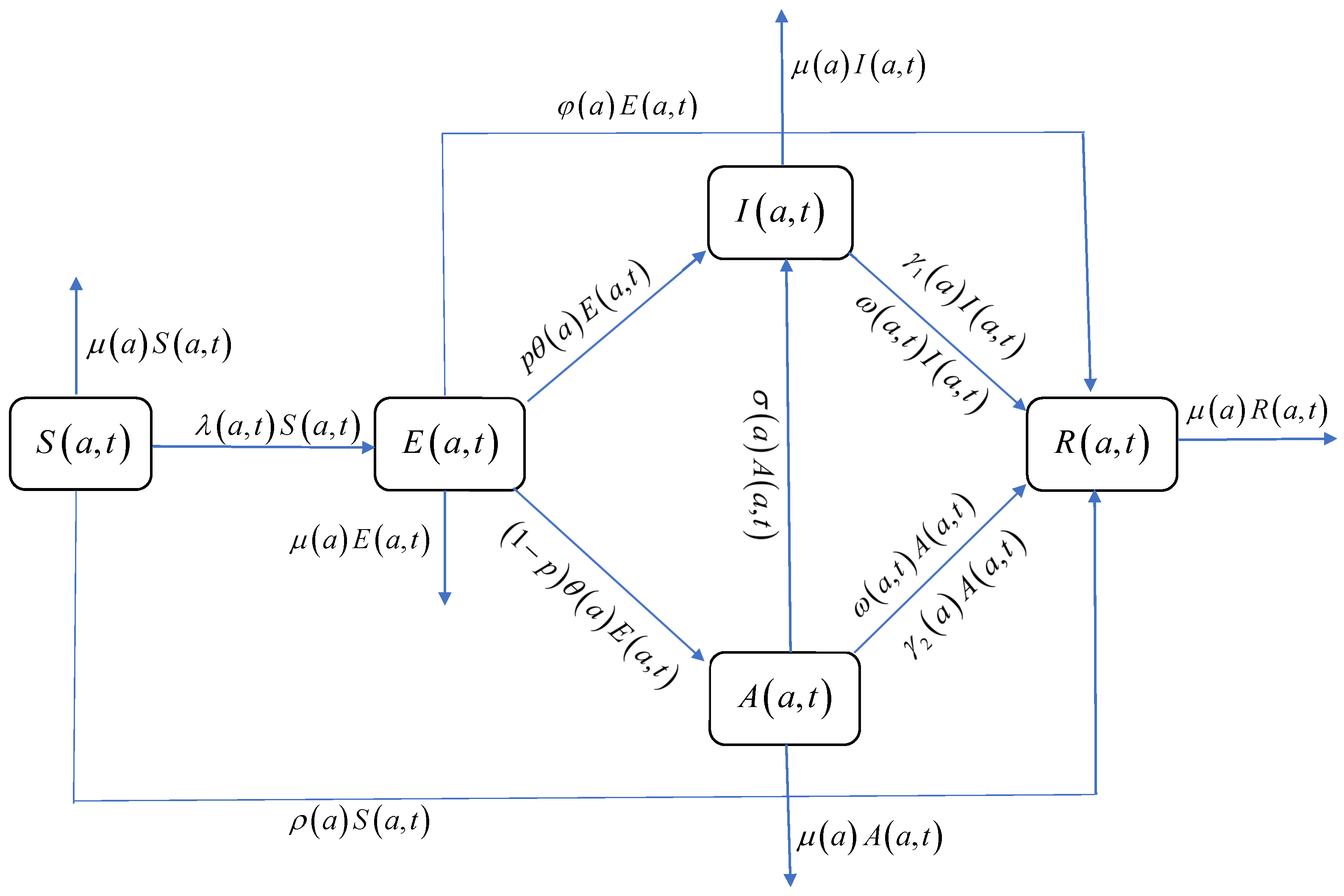
Furthermore, self-examination enables the earlier detection of infections, significantly reducing diagnosis time and facilitating prompt treatment. This proactive approach not only enhances recovery rates but also exhibits a positive correlation with the contemporaneous proportion of infected individuals in the population. Therefore, the recovery rates ${\gamma }_1$ and ${\gamma }_2$ become ${\gamma }_1+\omega (a,t)$ and ${\gamma }_2+\omega (a,t)$, respectively. Here, $\omega (a,t)=c\left(a\right)(1+i_1\left(t\right))$, $c\left(a\right)$ represents the increased recovery rate due to prompt treatment after learning about the disease from the media, and $i_1\left(t\right)$ represents the total proportion of infections at time t. The interactions between these state variables are shown in the flowchart of the model (Figure 1).

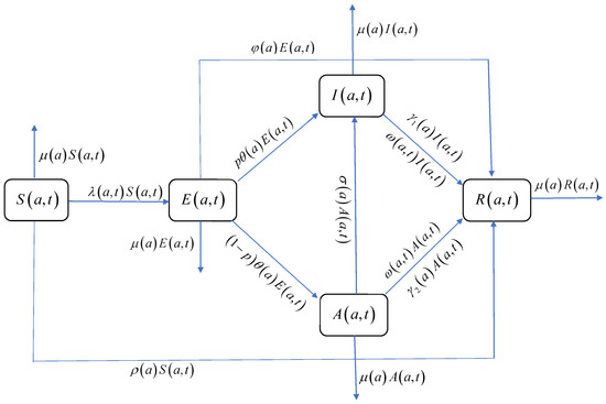
Figure 1. Flowchart of the model.

From an epidemiological modeling perspective, we establish the following system of partial differential equations:

$$\left\{\begin{array}{c}{\displaystyle \frac{\partial S}{\partial a}}+{\displaystyle \frac{\partial S}{\partial t}}=-S\left(a,t\right){\int }_0^{a^{+}}\beta \left(a,a^{\prime }\right){\displaystyle \frac{I\left(a^{\prime },t\right)+kA(a^{\prime },t)}{N(a^{\prime },t)}}d{a}^{\prime }-[\mu \left(a\right)+\rho \left(a\right)]S(a,t),\hfill \\ {\displaystyle \frac{\partial E}{\partial a}}+{\displaystyle \frac{\partial E}{\partial t}}=S\left(a,t\right){\int }_0^{a^{+}}\beta \left(a,a^{\prime }\right){\displaystyle \frac{I\left(a^{\prime },t\right)+kA(a^{\prime },t)}{N(a^{\prime },t)}}d{a}^{\prime }-[\mu \left(a\right)+\theta \left(a\right)+\phi \left(a\right)]E\left(a,t\right),\hfill \\ {\displaystyle \frac{\partial I}{\partial a}}+{\displaystyle \frac{\partial I}{\partial t}}=p\theta \left(a\right)E\left(a,t\right)+\sigma \left(a\right)A\left(a,t\right)-\left[\mu \left(a\right)+{\gamma }_1\left(a\right)+\omega \left(a,t\right)\right]I\left(a,t\right),\hfill \\ {\displaystyle \frac{\partial A}{\partial a}}+{\displaystyle \frac{\partial A}{\partial t}}=\left(1-p\right)\theta \left(a\right)E\left(a,t\right)-\left[{\gamma }_2\left(a\right)+\omega \left(a,t\right)+\sigma \left(a\right)+\mu \left(a\right)\right]A\left(a,t\right),\hfill \\ {\displaystyle \frac{\partial R}{\partial a}}+{\displaystyle \frac{\partial R}{\partial t}}=\phi \left(a\right)E\left(a,t\right)+\left[{\gamma }_1\left(a\right)+\omega \left(a,t\right)\right]I\left(a,t\right)\hfill \\ +\left[{\gamma }_2\left(a\right)+\omega \left(a,t\right)\right]A\left(a,t\right)-\mu \left(a\right)R\left(a,t\right)+\rho \left(a\right)S\left(a,t\right)\hfill \end{array}\right.$$

(1)

with initial value conditions (IVCs)

$$S(a,0)=S_0\left(a\right),E(a,0)=E_0\left(a\right),I(a,0)=I_0\left(a\right),A(a,0)=A_0\left(a\right),R(a,0)=R_0\left(a\right)$$

and boundary value conditions (BVCs) $S(0,t)=S^0\left(t\right)$, $E(0,t)=I(0,t)=A(0,t)=R(0,t)=0$.

Detailed biological considerations of the parameters of the model (1) can be found in Table 1.

Table 1. Summary of model parameters.

Parameter	Meaning
$\mu \left(a\right)$	Natural mortality rate related to age a
$\rho \left(a\right)$	Vaccine success rate for age a
$\theta \left(a\right)$	Reciprocal of the disease incubation period
$\phi \left(a\right)$	Self-cure rate of latent individuals due to media coverage
k	The relative infectiousness of asymptomatic individuals compared to symptomatic individuals
M	Initial population
$l\left(a\right)$	Average likelihood of being infected by contact with infected individuals of age a
$\tilde{\beta }\left(b\right)$	Average contact rate for a specific age
$\beta (a,b)$	Probability that a susceptible individual of age a is infected by an infected individual of age b

The primary objective of this study was to investigate the existence and stability conditions of both disease-free and endemic equilibrium states in system (1). For this purpose, we formulate the following well-founded assumptions considering human activity patterns and age demographics. Analogous assumptions can be found in references [20,21].

Assumption 1.

We provide the following assumptions throughout the paper:

(A1) Population sizes without immigration and emigration are set at a certain level.

(A2) Deaths due to disease are not considered.

(A3) Both asymptomatic and symptomatic individuals are infectious with an infection rate of β, and the infection rate of asymptomatic individuals is k times that of symptomatic individuals.

(A4) ${\int }_0^{a^{+}}\mu \left(a\right)da=+\infty$, which ensures no possibility of survival at the maximum age.

Using the same argument as that in [21] with obvious changes, we may prove the following:

Lemma 1.

The total population $N(a,t)$ is bounded if $N_0\left(a\right)$ and $S^0\left(t\right)$ are bounded.

To simplify system (1), a normalization transformation is applied. Let

$$s\left(a,t\right)={\displaystyle \frac{S\left(a,t\right)}{N\left(a,t\right)}},e\left(a,t\right)={\displaystyle \frac{E\left(a,t\right)}{N\left(a,t\right)}},i\left(a,t\right)={\displaystyle \frac{I\left(a,t\right)}{N\left(a,t\right)}},f\left(a,t\right)={\displaystyle \frac{A\left(a,t\right)}{N\left(a,t\right)}},r\left(a,t\right)={\displaystyle \frac{R\left(a,t\right)}{N\left(a,t\right)}}.$$

Then, system (1) takes the following form:

$$\left\{\begin{array}{c}{\displaystyle \frac{\partial s}{\partial a}+\frac{\partial s}{\partial t}=-[\lambda (a,t)+\rho \left(a\right)]s(a,t),}\hfill \\ {\displaystyle \frac{\partial e}{\partial a}+\frac{\partial e}{\partial t}=\lambda (a,t)s(a,t)-\left[\theta \left(a\right)+\phi \left(a\right)\right]e(a,t),}\hfill \\ {\displaystyle \frac{\partial i}{\partial a}+\frac{\partial i}{\partial t}=p\theta \left(a\right)e(a,t)+\sigma \left(a\right)f\left(a,t\right)-\left[{\gamma }_1\left(a\right)+\omega \left(a,t\right)\right]i\left(a,t\right),}\hfill \\ {\displaystyle \frac{\partial f}{\partial a}+\frac{\partial f}{\partial t}=\left(1-p\right)\theta \left(a\right)e(a,t)-\left[\sigma \left(a\right)+{\gamma }_2\left(a\right)+\omega \left(a,t\right)\right]f(a,t),}\hfill \\ {\displaystyle \frac{\partial r}{\partial a}+\frac{\partial r}{\partial t}=\phi \left(a\right)e\left(a,t\right)+\left[{\gamma }_1\left(a\right)+\omega \left(a,t\right)\right]i\left(t,a\right)}\hfill \\ {\displaystyle +\left[{\gamma }_2\left(a\right)+\omega \left(a,t\right)\right]f\left(a,t\right)+\rho \left(a\right)s\left(a,t\right)}\hfill \end{array}\right.$$

(2)

with IVCs

$$s(a,0)=s_0\left(a\right),e(a,0)=e_0\left(a\right),i(a,0)=i_0\left(a\right),f(a,0)=f_0\left(a\right),r(a,0)=r_0\left(a\right)$$

and BVCs $s(0,t)=1$, $e(0,t)=i(0,t)=f(0,t)=r(0,t)=0$, where

$$\lambda (a,t)=z\left(a\right){\int }_0^{a^{+}}\tilde{\beta }\left(a^{\prime }\right)[i(a^{\prime },t)+kf(a^{\prime },t)]d{a}^{\prime },z\left(a\right)={\displaystyle \frac{l\left(a\right)}{1+h{e}^{j+m\left(a\right)q\left(a\right)}}}.$$

3. Stability of the Disease-Free Steady State

This section focuses on establishing the existence and stability of the disease-free steady state in system (2). Since $s(a,t)+e(a,t)+i(a,t)+f(a,t)+r(a,t)=1$, system (2) can be simplified as follows:

$$\left\{\begin{array}{c}{\displaystyle \frac{\partial s}{\partial a}+\frac{\partial s}{\partial t}=-[\lambda (a,t)+\rho \left(a\right)]s(a,t),}\hfill \\ {\displaystyle \frac{\partial e}{\partial a}+\frac{\partial e}{\partial t}=\lambda (a,t)s(a,t)-\left[\theta \left(a\right)+\phi \left(a\right)\right]e(a,t),}\hfill \\ {\displaystyle \frac{\partial i}{\partial a}+\frac{\partial i}{\partial t}=p\theta \left(a\right)e(a,t)+\sigma \left(a\right)f\left(a,t\right)-\left[{\gamma }_1\left(a\right)+\omega \left(a,t\right)\right]i\left(a,t\right),}\hfill \\ {\displaystyle \frac{\partial f}{\partial a}+\frac{\partial f}{\partial t}=\left(1-p\right)\theta \left(a\right)e(a,t)-\left[\sigma \left(a\right)+{\gamma }_2\left(a\right)+\omega \left(a,t)\right)\right]f(a,t).}\hfill \end{array}\right.$$

(3)

Due to the time independence of the disease-free steady state, system (3) reduces to the following equations:

$$\left\{\begin{array}{c}{\displaystyle \frac{ds}{da}=-[\lambda \left(a\right)+\rho \left(a\right)]s\left(a\right),}\hfill \\ {\displaystyle \frac{de}{da}=\lambda \left(a\right)s\left(a\right)-\left[\theta \left(a\right)+\phi \left(a\right)\right]e\left(a\right),}\hfill \\ {\displaystyle \frac{di}{da}=p\theta \left(a\right)e\left(a\right)+\sigma \left(a\right)f\left(a\right)-\left[{\gamma }_1\left(a\right)+\omega \left(a\right)\right]i\left(a\right),}\hfill \\ {\displaystyle \frac{df}{da}=\left(1-p\right)\theta \left(a\right)e\left(a\right)-\left[\sigma \left(a\right)+{\gamma }_2\left(a\right)+\omega \left(a\right)\right]f\left(a\right)}\hfill \end{array}\right.$$

(4)

with IVCs $s\left(0\right)=1,e\left(0\right)=i\left(0\right)=f\left(0\right)=0,$ where

$$\lambda \left(a\right)=z\left(a\right){\int }_0^{a^{+}}\tilde{\beta }\left(b\right)\left[i\left(b\right)+kf\left(b\right)\right]db.$$

For the disease-free equilibrium $E^0=(s^0\left(a\right),e^0\left(a\right),i^0\left(a\right),f^0\left(a\right))$, then $i^0\left(a\right)=f^0\left(a\right)=0$, it is implied that $e^0\left(a\right)=0,\lambda \left(a\right)=0.$ Thus, $s^0\left(a\right)=e^{-{\int }_0^a\rho \left(s\right)ds}.$

In summary, it can be seen that the disease-free equilibrium exists and is unique; that is, $E^0=(s^0\left(a\right),0,0,0).$ For the purpose of studying the local stability of $E^0$, a linear transformation is performed on system (3) as follows:

$$\overline{s}(a,t)=s(a,t)-s^0\left(a\right),\overline{e}(a,t)=e(a,t),\overline{i}(a,t)=i(a,t),\overline{f}(a,t)=f(a,t).$$

Then, the linear part of the corresponding system is as follows:

$$\left\{\begin{array}{c}{\displaystyle \frac{\partial \overline{s}}{\partial a}+\frac{\partial \overline{s}}{\partial t}=-\rho \left(a\right)\overline{s}(a,t)-\overline{\lambda }(a,t)s^0\left(a\right),}\hfill \\ {\displaystyle \frac{\partial \overline{e}}{\partial a}+\frac{\partial \overline{e}}{\partial t}=\overline{\lambda }(a,t)s^0\left(a\right)-\left[\theta \left(a\right)+\phi \left(a\right)\right]\overline{e}(a,t),}\hfill \\ {\displaystyle \frac{\partial \overline{i}}{\partial a}+\frac{\partial \overline{i}}{\partial t}=p\theta \left(a\right)\overline{e}(a,t)+\sigma \left(a\right)\overline{f}\left(a,t\right)-\left[{\gamma }_1\left(a\right)+c\left(a\right)\right]\overline{i}(a,t),}\hfill \\ {\displaystyle \frac{\partial \overline{f}}{\partial a}+\frac{\partial \overline{f}}{\partial t}=\left(1-p\right)\theta \left(a\right)\overline{e}(a,t)-\left[\sigma \left(a\right)+{\gamma }_2\left(a\right)+c\left(a\right)\right]\overline{f}(a,t)}\hfill \end{array}\right.$$

(5)

with BVCs $\overline{s}(0,t)=\overline{e}(0,t)=\overline{i}(0,t)=\overline{f}(0,t)=0$, where

$$\lambda \left(a,t\right)=z\left(a\right){\int }_0^{a^{+}}\tilde{\beta }\left(b\right)\left[\overline{i}\left(b,t\right)+k\overline{f}\left(b,t\right)\right]db.$$

Consider the exponential solution form of system (5),

$$s(a,t)=\overline{s}\left(a\right)e^{mt},\overline{e}(a,t)=\overline{e}\left(a\right)e^{mt},\overline{i}(a,t)=\overline{i}\left(a\right)e^{mt},\overline{f}(a,t)=\overline{f}\left(a\right)e^{mt}.$$

System (5) takes the following form

$$\left\{\begin{array}{c}{\displaystyle \frac{d\overline{s}}{da}=-\overline{\lambda }\left(a\right)s^0\left(a\right)-[\rho \left(a\right)+m]\overline{s}\left(a\right),}\hfill \\ {\displaystyle \frac{d\overline{e}}{da}=\overline{\lambda }\left(a\right)s^0\left(a\right)-[\theta \left(a\right)+\phi \left(a\right)+m]\overline{e}\left(a\right),}\hfill \\ {\displaystyle \frac{d\overline{i}}{da}=p\theta \left(a\right)\overline{e}\left(a\right)+\sigma \left(a\right)\overline{f}\left(a\right)-[{\gamma }_1\left(a\right)+c\left(a\right)+m]\overline{i}\left(a\right),}\hfill \\ {\displaystyle \frac{d\overline{f}}{da}=\left(1-p\right)\theta \left(a\right)\overline{e}\left(a\right)-[\sigma \left(a\right)+{\gamma }_2\left(a\right)+c\left(a\right)+m]\overline{f}\left(a\right)}\hfill \end{array}\right.$$

(6)

with IVCs $\overline{s}\left(0\right)=\overline{e}\left(0\right)=\overline{i}\left(0\right)=\overline{f}\left(0\right)=0,$ where

$$\overline{\lambda }\left(a\right)=z\left(a\right){\int }_0^{a^{+}}\tilde{\beta }\left(b\right)[\overline{i}\left(b\right)+k\overline{f}\left(b\right)]db.$$

If we let $\mathsf{\Lambda }={\int }_0^{a^{+}}\tilde{\beta }\left(b\right)[\overline{i}\left(b\right)+k\overline{f}\left(b\right)]db$, then $\overline{\lambda }\left(a\right)=z\left(a\right)\mathsf{\Lambda }.$ Therefore, we obtain the solution of system (6) below:

$$\left\{\begin{array}{c}{\displaystyle \overline{s}\left(a\right)=-\mathsf{\Lambda }{\int }_0^{a}z\left(\tau \right)s^0\left(\tau \right)e^{-{\int }_{\tau }^a[\rho \left(s\right)+m]ds}d\tau ,}\hfill \\ {\displaystyle \overline{e}\left(a\right)=\mathsf{\Lambda }{\int }_0^{a}z\left(\tau \right)s^0\left(\tau \right)e^{-{\int }_{\tau }^a[\theta \left(s\right)+\phi \left(s\right)+m]ds}d\tau ,}\hfill \\ {\displaystyle \overline{i}\left(a\right)={\int }_0^a\left[p\theta \left(\tau \right)\overline{e}\left(\tau \right)+\sigma \left(\tau \right)\overline{f}\left(\tau \right)\right]e^{-{\int }_{\tau }^a[{\gamma }_1\left(s\right)+c\left(s\right)+m]ds}d\tau ,}\hfill \\ {\displaystyle \overline{f}\left(a\right)={\int }_0^a\left[\left(1-p\right)\theta \left(\tau \right)\overline{e}\left(\tau \right)\right]e^{-{\int }_{\tau }^a[\sigma \left(s\right)+{\gamma }_2\left(s\right)+c\left(s\right)+m]ds}d\tau .}\hfill \end{array}\right.$$

Substituting $\overline{f}\left(a\right)$ and $\overline{i}\left(a\right)$ into $\mathsf{\Lambda }$, we have

$$\mathsf{\Lambda }=\mathsf{\Lambda }\left(\begin{array}{c}{\int }_0^{a^{+}}\tilde{\beta }\left(b\right){\int }_0^{b}Y(\tau ,b)\left[\begin{array}{c}{\displaystyle p\theta \left(\tau \right){\int }_0^{\tau }z\left(\xi \right)s^0\left(\xi \right)X(\xi ,\tau )e^{-m(b-\xi )}+\left(1-p\right)\sigma \left(\tau \right)}\hfill \\ {\displaystyle {\int }_0^{\tau }\theta \left(\xi \right)Z(\xi ,\tau ){\int }_0^{\xi }z\left(\eta \right)s^0\left(\eta \right)X(\eta ,\xi )e^{-m(b-\eta )}d\eta }\hfill \end{array}\right]d\xi d\tau db\hfill \\ {\displaystyle +k\left(1-p\right){\int }_0^{a^{+}}\tilde{\beta }\left(b\right){\int }_0^b\theta \left(\tau \right)Z(\tau ,b){\int }_0^{\tau }z\left(\xi \right)s^0\left(\xi \right)X(\xi ,\tau )e^{-m(b-\xi )}d\xi d\tau db}\hfill \end{array}\right),$$

Thus, the characteristic equation is

$$\begin{array}{c}1={\int }_0^{a^{+}}\tilde{\beta }\left(b\right){\int }_0^{b}Y(\tau ,b)\left[\begin{array}{c}{\displaystyle p\theta \left(\tau \right){\int }_0^{\tau }z\left(\xi \right)s^0\left(\xi \right)X(\xi ,\tau )e^{-m(b-\xi )}+\left(1-p\right)\sigma \left(\tau \right)}\hfill \\ {\displaystyle {\int }_0^{\tau }\theta \left(\xi \right)Z(\xi ,\tau ){\int }_0^{\xi }z\left(\eta \right)s^0\left(\eta \right)X(\eta ,\xi )e^{-m(b-\eta )}d\eta }\hfill \end{array}\right]d\xi d\tau db\hfill \\ {\displaystyle +k\left(1-p\right){\int }_0^{a^{+}}\tilde{\beta }\left(b\right){\int }_0^b\theta \left(\tau \right)Z(\tau ,b){\int }_0^{\tau }z\left(\xi \right)s^0\left(\xi \right)X(\xi ,\tau )e^{-m(b-\xi )}d\xi d\tau db,}\hfill \end{array}$$

where $X(\xi ,\tau )=e^{-{\int }_{\xi }^{\tau }\left[\theta \left(s\right)+\phi \left(s\right)\right]ds},Y(\tau ,b)=e^{-{\int }_{\tau }^b\left[{\gamma }_1\left(s\right)+c\left(s\right)\right]ds},Z(\tau ,b)=e^{-{\int }_{\tau }^b\left[\sigma \left(s\right)+{\gamma }_2\left(s\right)+c\left(s\right)\right]ds}.$

Denote

$$\begin{array}{c}F\left(m\right)={\int }_0^{a^{+}}\tilde{\beta }\left(b\right){\int }_0^{b}Y(\tau ,b)\left[\begin{array}{c}p\theta \left(\tau \right){\int }_0^{\tau }z\left(\xi \right)s^0\left(\xi \right)X(\xi ,\tau )e^{-m(b-\xi )}+\left(1-p\right)\sigma \left(\tau \right)\hfill \\ {\int }_0^{\tau }\theta \left(\xi \right)Z(\xi ,\tau ){\int }_0^{\xi }z\left(\eta \right)s^0\left(\eta \right)X(\eta ,\xi )e^{-m(b-\eta )}d\eta \hfill \end{array}\right]d\xi d\tau db\hfill \\ +k\left(1-p\right){\int }_0^{a^{+}}\tilde{\beta }\left(b\right){\int }_0^b\theta \left(\tau \right)Z(\tau ,b){\int }_0^{\tau }z\left(\xi \right)s^0\left(\xi \right)X(\xi ,\tau )e^{-m(b-\xi )}d\xi d\tau db.\hfill \end{array}$$

Let the basic reproduction number $R_0=F\left(0\right)$; that is,

$$\begin{array}{c}{\displaystyle R_0={\int }_0^{a^{+}}\tilde{\beta }\left(b\right){\int }_0^{b}Y(\tau ,b)\left[\begin{array}{c}{\displaystyle p\theta \left(\tau \right){\int }_0^{\tau }z\left(\xi \right)s^0\left(\xi \right)X(\xi ,\tau )+\left(1-p\right)\sigma \left(\tau \right)}\hfill \\ {\displaystyle {\int }_0^{\tau }\theta \left(\xi \right)Z(\xi ,\tau ){\int }_0^{\xi }z\left(\eta \right)s^0\left(\eta \right)X(\eta ,\xi )d\eta }\hfill \end{array}\right]d\xi d\tau db}\hfill \\ {\displaystyle +k\left(1-p\right){\int }_0^{a^{+}}\tilde{\beta }\left(b\right){\int }_0^b\theta \left(\tau \right)Z(\tau ,b){\int }_0^{\tau }z\left(\xi \right)s^0\left(\xi \right)X(\xi ,\tau )d\xi d\tau db.}\hfill \end{array}$$

(7)

Theorem 1.

The disease-free steady state $E^0$ is locally asymptotically stable if $R_0<1$ and unstable if $R_0>1$.

Proof. 

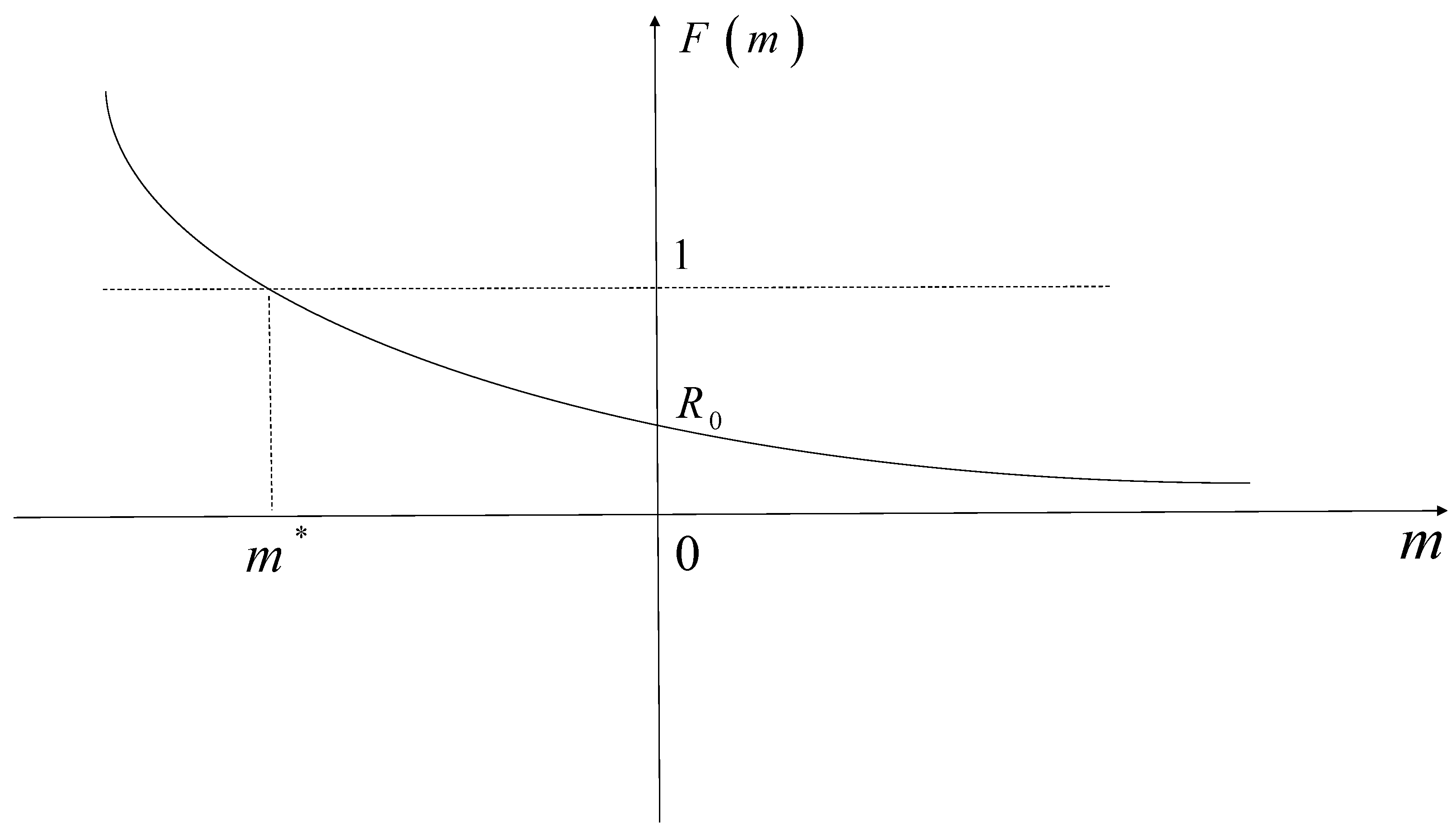
We can obtain some properties of the function $F\left(m\right)$:

$$F^{\prime }\left(m\right)<0,\underset{m\to -\infty }{lim}F\left(m\right)=+\infty ,\underset{m\to +\infty }{lim}F\left(m\right)=0.$$

Then, the equation $F\left(m\right)=1$ has a unique real root $m^{\ast }$.

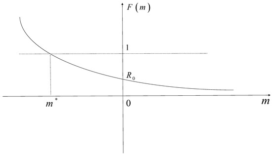
Case 1: The equation $F\left(m\right)=1$ has exactly one root, so the root must be $m^{\ast }$. Therefore, the root $m^{\ast }$ is negative provided $R_0<1$, as shown in Figure 2.

Figure 2. The graph of $F\left(m\right)$.

Case 2: The equation $F\left(m\right)=1$ has complex roots $u=\alpha +i\beta$. If $R_0<1$, then

$$F\left(m^{\ast }\right)=1=\mathrm{Re}F\left(u\right)=\mathrm{Re}F(\alpha +i\beta )\le F\left(\alpha \right),$$

and if F monotonically decreases, it follows that $\alpha \le m^{\ast }<0$.

Based on the above discussion, the roots of the equation $F\left(m\right)=1$ always have negative real parts provided $R_0<1$, which yields $E^0$, which is locally asymptotically stable if $R_0<1$.

Similarly, we can prove that $E^0$ is unstable if $R_0>1$. □

Theorem 2.

The disease-free steady state $E^0$ is globally asymptotically stable if $R_0<1$.

Proof. 

According to the definition of global stability, we will show

$$\begin{array}{l}\underset{t\to \infty }{lim}s(a,t)=s^0\left(a\right)=e^{-{\int }_0^a\rho \left(s\right)ds},\underset{t\to \infty }{lim}e(a,t)=e^0\left(a\right)=0,\\ \underset{t\to \infty }{lim}i(a,t)=i^0\left(a\right)=0,\underset{t\to \infty }{lim}f(a,t)=f^0\left(a\right)=0.\end{array}$$

(8)

Therefore, it suffices to discuss the solutions when $t>a$. The first equation of system (3) is integrated along the characteristic line $a=t+c$ if $t>a$, meaning that

$$s(a,t)=e^{-{\int }_0^a\left[\lambda \left(s,s-a+t\right)+\rho \left(s\right)\right]ds}.$$

Similarly, we have

$$\begin{array}{l}e(a,t)={\int }_0^a\lambda \left(\tau ,\tau -a+t\right)s\left(\tau ,\tau -a+t\right)e^{-{\int }_{\tau }^a\left[\theta \left(s\right)+\phi \left(s\right)\right]ds}d\tau ,\\ i\left(a,t\right)={\int }_0^a{e}^{-{\int }_{\tau }^a\left[{\gamma }_1\left(s\right)+\omega \left(s,s-a+t\right)\right]ds}\left[p\theta \left(\tau \right)e\left(\tau ,\tau -a+t\right)+\sigma \left(\tau \right)f\left(\tau ,\tau -a+t\right)\right]d\tau ,\\ f\left(a,t\right)={\int }_0^a{e}^{-{\int }_{\tau }^a\left[\sigma \left(s\right)+{\gamma }_2\left(s\right)+\omega \left(s,s-a+t\right)\right]ds}\left[\left(1-p\right)\theta \left(\tau \right)e\left(\tau ,\tau -a+t\right)\right]d\tau .\end{array}$$

Let $\chi \left(t\right)={\int }_0^{a^{+}}\tilde{\beta }\left(b\right)[i(b,t)+kf(b,t)]db$. Then, $\lambda (a,t)=z\left(a\right)\chi \left(t\right)$ and

$$\begin{array}{l}\chi \left(t\right)={\int }_0^{a^{+}}\tilde{\beta }\left(b\right){\int }_0^b{e}^{-{\int }_{\tau }^b\left[{\gamma }_1\left(s\right)+\omega \left(s,s-b+t\right)\right]ds}\\ \left[\begin{array}{c}{\displaystyle p\theta \left(\tau \right){\int }_0^{\tau }\lambda \left(\xi ,\xi -b+t\right)s\left(\xi ,\xi -b+t\right)X(\xi ,\tau )}\hfill \\ {\displaystyle +\left(1-p\right)\sigma \left(\tau \right){\int }_0^{\tau }{e}^{-{\int }_{\xi }^{\tau }\left[\sigma \left(s\right)+{\gamma }_2\left(s\right)+\omega \left(s,s-b+t\right)\right]ds}\theta \left(\xi \right)}\hfill \\ {\displaystyle {\int }_0^{\xi }\lambda \left(\eta ,\eta -b+t\right)s\left(\eta ,\eta -b+t\right)X(\eta ,\xi )d\eta }\hfill \end{array}\right]d\xi d\tau db\\ +k\left(1-p\right){\int }_0^{a^{+}}\tilde{\beta }\left(b\right){\int }_0^b{e}^{-{\int }_{\tau }^b\left[\sigma \left(s\right)+{\gamma }_2\left(s\right)+\omega \left(s,s-b+t\right)\right]ds}\theta \left(\tau \right)\\ {\int }_0^{\tau }\lambda \left(\xi ,\xi -b+t\right)s\left(\xi ,\xi -b+t\right)X(\xi ,\tau )d\xi d\tau db\\ ={\int }_0^{a^{+}}\tilde{\beta }\left(b\right){\int }_0^b{e}^{-{\int }_{\tau }^b\left[{\gamma }_1\left(s\right)+\omega \left(s,s-b+t\right)\right]ds}\\ \left[\begin{array}{c}{\displaystyle p\theta \left(\tau \right){\int }_0^{\tau }z\left(\xi \right)\chi \left(\xi -b+t\right)s\left(\xi ,\xi -b+t\right)X(\xi ,\tau )}\hfill \\ {\displaystyle +\left(1-p\right)\sigma \left(\tau \right){\int }_0^{\tau }{e}^{-{\int }_{\xi }^{\tau }\left[\sigma \left(s\right)+{\gamma }_2\left(s\right)+\omega \left(s,s-b+t\right)\right]ds}\theta \left(\xi \right)}\hfill \\ {\displaystyle {\int }_0^{\xi }z\left(\eta \right)\chi \left(\eta -b+t\right)s\left(\eta ,\eta -b+t\right)X(\eta ,\xi )d\eta }\hfill \end{array}\right]d\xi d\tau db\\ +k\left(1-p\right){\int }_0^{a^{+}}\tilde{\beta }\left(b\right){\int }_0^b{e}^{-{\int }_{\tau }^b\left[\sigma \left(s\right)+{\gamma }_2\left(s\right)+\omega \left(s,s-b+t\right)\right]ds}\theta \left(\tau \right)\\ {\int }_0^{\tau }z\left(\xi \right)\chi \left(\xi -b+t\right)s\left(\xi ,\xi -b+t\right)X(\xi ,\tau )d\xi d\tau db.\end{array}$$

Moreover, $\lambda (a,t)\ge 0$ and $i_1\left(t\right)\ge 0$ yield

$$\begin{array}{l}s(\xi ,\xi -b+t)=e^{-{\int }_0^{\xi }\left[\lambda \right(s,s-b+t)+\rho (s\left)\right]ds}\le e^{-{\int }_0^{\xi }\rho \left(s\right)ds}=s^0\left(\xi \right),\\ s(\eta ,\eta -b+t)=e^{-{\int }_0^{\eta }\left[\lambda \right(s,s-b+t)+\rho (s\left)\right]ds}\le e^{-{\int }_0^{\eta }\rho \left(s\right)ds}=s^0\left(\eta \right),\\ \omega \left(s,s-b+t\right)=c\left(s\right)(1+i_1(s-b+t))\ge c\left(s\right).\end{array}$$

Thus,

$$\begin{array}{ll}\chi \left(t\right)\le & {\int }_0^{a^{+}}\tilde{\beta }\left(b\right){\int }_0^{b}Y(\tau ,b)\left[\begin{array}{c}p\theta \left(\tau \right){\int }_0^{\tau }z\left(\xi \right)\chi \left(\xi -b+t\right)s^0\left(\xi \right)X(\xi ,\tau )\hfill \\ +\left(1-p\right)\sigma \left(\tau \right){\int }_0^{\tau }\theta \left(\xi \right)Z(\xi ,\tau )\hfill \\ {\int }_0^{\xi }z\left(\eta \right)\chi \left(\eta -b+t\right)s^0\left(\eta \right)X(\eta ,\xi )d\eta \hfill \end{array}\right]d\xi d\tau db\\ & +k\left(1-p\right){\int }_0^{a^{+}}\tilde{\beta }\left(b\right){\int }_0^b\theta \left(\tau \right)Z(\tau ,b){\int }_0^{\tau }z\left(\xi \right)\chi \left(\xi -b+t\right)s^0\left(\xi \right)X(\xi ,\tau )d\xi d\tau db.\end{array}$$

(9)

Combining (7) and (9), we obtain

$$\underset{t\to \infty }{lim}sup\chi \left(t\right)\le R_0\underset{t\to \infty }{lim}sup\chi \left(t\right).$$

When $R_0<1$, we have

$$\underset{t\to \infty }{lim}sup\chi \left(t\right)=0$$

due to the non-negativity of $\chi \left(t\right).$ It follows from $\chi \left(t\right)={\int }_0^{a^{+}}\tilde{\beta }\left(a\right)[i(a,t)+kf(a,t)]da$ that

$${\displaystyle \underset{t\to \infty }{lim}sup[i(a,t)+kf(a,t)]=0,\underset{t\to \infty }{lim}supi(a,t)=0,\underset{t\to \infty }{lim}supf(a,t)=0.}$$

It is easy to see from the expression $i(a,t)$ or $f\left(a,t\right)$ that $\underset{t\to \infty }{lim}supe(a,t)=0,$

$$\begin{array}{ll}\underset{t\to \infty }{lim}sups(a,t)& =\underset{t\to \infty }{lim}sup{e}^{-{\int }_0^a\left[\lambda \left(s,s-a+t\right)+\rho \left(s\right)\right]ds}\\ & =\underset{t\to \infty }{lim}sup{e}^{-{\int }_0^a\left[z\right(s\left)\chi \right(s-a+t)+\rho (s\left)\right]ds}\\ & =e^{-{\int }_0^a\rho \left(s\right)ds}=s^0\left(a\right).\end{array}$$

Thus, we end the proof. □

4. Stability of the Endemic Steady State

When system (3) attains a stable age-distribution, it depends solely on a. That is, the steady-state solution of system (3) satisfies the following form:

$$\left\{\begin{array}{c}{\displaystyle \frac{d{s}^{\ast }\left(a\right)}{da}=-[{\lambda }^{\ast }\left(a\right)+\rho \left(a\right)]s^{\ast }\left(a\right),}\hfill \\ {\displaystyle \frac{d{e}^{\ast }\left(a\right)}{da}={\lambda }^{\ast }\left(a\right)s^{\ast }\left(a\right)-\left[\theta \left(a\right)+\phi \left(a\right)\right]e^{\ast }\left(a\right),}\hfill \\ {\displaystyle \frac{d{i}^{\ast }\left(a\right)}{da}=p\theta \left(a\right)e^{\ast }\left(a\right)+\sigma \left(a\right)f^{\ast }\left(a\right)-\left[{\gamma }_1\left(a\right)+c\left(a\right)\right]i^{\ast }\left(a\right),}\hfill \\ {\displaystyle \frac{d{f}^{\ast }\left(a\right)}{da}=\left(1-p\right)\theta \left(a\right)e^{\ast }\left(a\right)-\left[\sigma \left(a\right)+{\gamma }_2\left(a\right)+c\left(a\right)\right]f^{\ast }\left(a\right)}\hfill \end{array}\right.$$

(10)

with IVCs $s^{\ast }\left(0\right)=1,e^{\ast }\left(0\right)=i^{\ast }\left(0\right)=f^{\ast }\left(0\right)=0,$ where

$${\lambda }^{\ast }\left(a\right)=z\left(a\right){\int }_0^{a^{+}}\tilde{\beta }\left(b\right)[i^{\ast }\left(b\right)+k{f}^{\ast }\left(b\right)]db=z\left(a\right){\mathsf{\Lambda }}^{\ast },{\mathsf{\Lambda }}^{\ast }={\int }_0^{a^{+}}\tilde{\beta }\left(b\right)[i^{\ast }\left(b\right)+k{f}^{\ast }\left(b\right)]db.$$

The solution of (10) is

$$\begin{array}{l}{s}^{\ast }\left(a\right)=e^{-{\int }_0^a[{\lambda }^{\ast }\left(s\right)+\rho \left(s\right)]ds}=e^{-{\int }_0^a[{\mathsf{\Lambda }}^{\ast }z\left(s\right)+\rho \left(s\right)]ds},\\ e^{\ast }\left(a\right)={\int }_0^a{\mathsf{\Lambda }}^{\ast }z\left(\tau \right)s^{\ast }\left(\tau \right)e^{-{\int }_{\tau }^a\left[\theta \left(s\right)+\phi \left(s\right)\right]ds}d\tau ,\\ i^{\ast }\left(a\right)={\int }_0^a\left[p\theta \left(\tau \right)e^{\ast }\left(\tau \right)+\sigma \left(\tau \right)f^{\ast }\left(\tau \right)\right]e^{-{\int }_{\tau }^a\left[{\gamma }_1\left(s\right)+c\left(s\right)\right]ds}d\tau ,\\ f^{\ast }\left(a\right)={\int }_0^a\left(1-p\right)\theta \left(\tau \right)e^{\ast }\left(\tau \right)e^{-{\int }_{\tau }^a\left[\sigma \left(s\right)+{\gamma }_2\left(s\right)+c\left(s\right)\right]ds}d\tau .\end{array}$$

It is not difficult to find that when ${\mathsf{\Lambda }}^{\ast }=0$, the endemic steady state $E^{\ast }$ becomes the disease-free steady state $E^0=(s^0\left(a\right),0,0,0)$.

For ${\mathsf{\Lambda }}^{\ast }\ne 0$, substituting the expressions of $s^{\ast }\left(a\right),e^{\ast }\left(a\right),i^{\ast }\left(a\right),f^{\ast }\left(a\right)$ into

$${\mathsf{\Lambda }}^{\ast }={\int }_0^{a^{+}}\tilde{\beta }\left(b\right)[i^{\ast }\left(b\right)+k{f}^{\ast }\left(b\right)]db$$

allows us to obtain the following:

$$\begin{array}{c}{\displaystyle 1={\int }_0^{a^{+}}\tilde{\beta }\left(b\right){\int }_0^{b}Y(\tau ,b)\left[\begin{array}{c}{\displaystyle p\theta \left(\tau \right){\int }_0^{\tau }z\left(\xi \right)e^{-{\int }_0^{\xi }\left[z\left(s\right){\mathsf{\Lambda }}^{\ast }+\rho \left(s\right)\right]ds}X(\xi ,\tau )+\left(1-p\right)\sigma \left(\tau \right)}\hfill \\ {\displaystyle {\int }_0^{\tau }\theta \left(\xi \right)Z(\xi ,\tau ){\int }_0^{\xi }z\left(\eta \right)e^{-{\int }_0^{\eta }\left[z\left(s\right){\mathsf{\Lambda }}^{\ast }+\rho \left(s\right)\right]ds}X(\eta ,\xi )d\eta }\hfill \end{array}\right]d\xi d\tau db}\hfill \\ {\displaystyle +k\left(1-p\right){\int }_0^{a^{+}}\tilde{\beta }\left(b\right){\int }_0^b\theta \left(\tau \right)Z(\tau ,b){\int }_0^{\tau }z\left(\xi \right)e^{-{\int }_0^{\xi }\left[z\left(s\right){\mathsf{\Lambda }}^{\ast }+\rho \left(s\right)\right]ds}X(\xi ,\tau )d\xi d\tau db.}\hfill \end{array}$$

Let the right-hand side of the above equation be denoted as $L\left({\mathsf{\Lambda }}^{\ast }\right)$; that is,

$$\begin{array}{c}{\displaystyle L\left({\mathsf{\Lambda }}^{\ast }\right)={\int }_0^{a^{+}}\tilde{\beta }\left(b\right){\int }_0^{b}Y(\tau ,b)\left[\begin{array}{c}{\displaystyle p\theta \left(\tau \right){\int }_0^{\tau }z\left(\xi \right)e^{-{\int }_0^{\xi }\left[z\left(s\right){\mathsf{\Lambda }}^{\ast }+\rho \left(s\right)\right]ds}X(\xi ,\tau )+\left(1-p\right)\sigma \left(\tau \right)}\hfill \\ {\displaystyle {\int }_0^{\tau }\theta \left(\xi \right)Z(\xi ,\tau ){\int }_0^{\xi }z\left(\eta \right)e^{-{\int }_0^{\eta }\left[z\left(s\right){\mathsf{\Lambda }}^{\ast }+\rho \left(s\right)\right]ds}X(\eta ,\xi )d\eta }\hfill \end{array}\right]d\xi d\tau db}\hfill \\ {\displaystyle +k\left(1-p\right){\int }_0^{a^{+}}\tilde{\beta }\left(b\right){\int }_0^b\theta \left(\tau \right)Z(\tau ,b){\int }_0^{\tau }z\left(\xi \right)e^{-{\int }_0^{\xi }\left[z\left(s\right){\mathsf{\Lambda }}^{\ast }+\rho \left(s\right)\right]ds}X(\xi ,\tau )d\xi d\tau db.}\hfill \end{array}$$

Then, there exists a unique endemic steady state if and only if there is a unique ${\mathsf{\Lambda }}^{\ast }$ such that $L\left({\mathsf{\Lambda }}^{\ast }\right)=1$ and ${\mathsf{\Lambda }}^{\ast }>0$. Consequently, we shall prove the following result:

Theorem 3.

If $R_0>1$, system (3) admits a unique endemic steady state $E^{\ast }$.

Proof. 

The properties of $L\left({\mathsf{\Lambda }}^{\ast }\right)$ are proved as follows:

$$L^{\prime }\left({\mathsf{\Lambda }}^{\ast }\right)<0,L\left(0\right)=R_0,\underset{{\mathsf{\Lambda }}^{\ast }\to -\infty }{lim}L\left({\mathsf{\Lambda }}^{\ast }\right)=+\infty ,$$

$$\underset{{\mathsf{\Lambda }}^{\ast }\to +\infty }{lim}L\left({\mathsf{\Lambda }}^{\ast }\right)=\underset{{\mathsf{\Lambda }}^{\ast }\to +\infty }{lim}{\displaystyle \frac{1}{{\mathsf{\Lambda }}^{\ast }}}{\int }_0^{a^{+}}\tilde{\beta }\left(b\right)\left[i^{\ast }\left(b\right)+k{f}^{\ast }\left(b\right)\right]db\le \underset{{\mathsf{\Lambda }}^{\ast }\to +\infty }{lim}{\displaystyle \frac{1+k}{{\mathsf{\Lambda }}^{\ast }}}{\int }_0^{a^{+}}\tilde{\beta }\left(b\right)db=0,$$

which implies that the equation $L\left({\mathsf{\Lambda }}^{\ast }\right)=1$ has a unique positive real root ${\mathsf{\Lambda }}_{\sim }^{\ast }$ if $R_0>1$. Then, system (3) has a unique positive steady state $E^{\ast }=(s^{\ast }\left(a\right),e^{\ast }\left(a\right),i^{\ast }\left(a\right),f^{\ast }\left(a\right))$, given by the expressions of $s^{\ast }\left(a\right),e^{\ast }\left(a\right),i^{\ast }\left(a\right),f^{\ast }\left(a\right)$ when ${\mathsf{\Lambda }}^{\ast }={\mathsf{\Lambda }}_{\sim }^{\ast }$. □

To analyze the local stability of the endemic steady state when $R_0>1$, we further need to study the linearized system of (3) at $E^{\ast }=(s^{\ast }\left(a\right),e^{\ast }\left(a\right),i^{\ast }\left(a\right),f^{\ast }\left(a\right))$. If we let

$$\begin{array}{l}\tilde{s}\left(a,t\right)=s\left(a,t\right)-s^{\ast }\left(a\right),\tilde{e}\left(a,t\right)=e\left(a,t\right)-e^{\ast }\left(a\right),\\ \tilde{i}\left(a,t\right)=i\left(a,t\right)-i^{\ast }\left(a\right),\tilde{f}\left(a,t\right)=f\left(a,t\right)-f^{\ast }\left(a\right),\end{array}$$

then the linear part of the corresponding system is as follows:

$$\left\{\begin{array}{c}{\displaystyle \frac{\partial \tilde{s}}{\partial a}+\frac{\partial \tilde{s}}{\partial t}=-\tilde{\lambda }\left(a,t\right)s^{\ast }\left(a\right)-{\lambda }^{\ast }\left(a\right)\tilde{s}\left(a,t\right)-\rho \left(a\right)\tilde{s}\left(a,t\right),}\hfill \\ {\displaystyle \frac{\partial \tilde{e}}{\partial a}+\frac{\partial \tilde{e}}{\partial t}=\tilde{\lambda }\left(a,t\right)s^{\ast }\left(a\right)+{\lambda }^{\ast }\left(a\right)\tilde{s}\left(a,t\right)-\left[\theta \left(a\right)+\phi \left(a\right)\right]\tilde{e}\left(a,t\right),}\hfill \\ {\displaystyle \frac{\partial \tilde{i}}{\partial a}+\frac{\partial \tilde{i}}{\partial t}=p\theta \left(a\right)\tilde{e}\left(a,t\right)+\sigma \left(a\right)\tilde{f}\left(a,t\right)-\left[{\gamma }_1\left(a\right)+c\left(a\right)\right]\tilde{i}\left(a,t\right),}\hfill \\ {\displaystyle \frac{\partial \tilde{f}}{\partial a}+\frac{\partial \tilde{f}}{\partial t}=\left(1-p\right)\theta \left(a\right)\tilde{e}\left(a,t\right)-\left[\sigma \left(a\right)+{\gamma }_2\left(a\right)+c\left(a\right)\right]\tilde{f}\left(a,t\right)}\hfill \end{array}\right.$$

(11)

with BVCs $\tilde{s}(0,t)=\tilde{e}(0,t)=\tilde{i}(0,t)=\tilde{f}(0,t)=0,$ where

$$\tilde{\lambda }\left(a,t\right)=z\left(a\right){\int }_0^{a^{+}}\tilde{\beta }\left(a^{\prime }\right)[\tilde{i}\left(a^{\prime },t\right)+k\tilde{f}\left(a^{\prime },t\right)]d{a}^{\prime }.$$

Consider the exponential solution form for the above system (11):

$$\tilde{s}\left(a,t\right)=\tilde{s}\left(a\right)e^{nt},\tilde{e}\left(a,t\right)=\tilde{e}\left(a\right)e^{nt},\tilde{i}\left(a,t\right)=\tilde{i}\left(a\right)e^{nt},\tilde{f}\left(a,t\right)=\tilde{f}\left(a\right)e^{nt},\tilde{r}\left(a,t\right)=\tilde{r}\left(a\right)e^{nt}.$$

Then,

$$\left\{\begin{array}{c}{\displaystyle \frac{d\tilde{s}}{da}=-\tilde{\mathsf{\Lambda }}z\left(a\right)s^{\ast }\left(a\right)-[{\lambda }^{\ast }\left(a\right)+\rho \left(a\right)+n]\tilde{s}\left(a\right),}\hfill \\ {\displaystyle \frac{d\tilde{e}}{da}=\tilde{\mathsf{\Lambda }}z\left(a\right){\tilde{s}}^{\ast }\left(a\right)+{\lambda }^{\ast }\left(a\right)\tilde{s}\left(a\right)-[\theta \left(a\right)+\phi \left(a\right)+n]\tilde{e}\left(a\right),}\hfill \\ {\displaystyle \frac{d\tilde{i}}{da}=p\theta \left(a\right)\tilde{e}\left(a\right)+\sigma \left(a\right)\tilde{f}\left(a\right)-\left[{\gamma }_1\left(a\right)+c\left(a\right)+n\right]\tilde{i}\left(a\right),}\hfill \\ {\displaystyle \frac{d\tilde{f}}{da}=\left(1-p\right)\theta \left(a\right)\tilde{e}\left(a\right)-\left[\sigma \left(a\right)+{\gamma }_2\left(a\right)+c\left(a\right)+n\right]\tilde{f}\left(a\right)}\hfill \end{array}\right.$$

(12)

with IVCs $\tilde{s}\left(0\right)=\tilde{e}\left(0\right)=\tilde{i}\left(0\right)=\tilde{f}\left(0\right)=0,$ where

$$\tilde{\mathsf{\Lambda }}={\int }_0^{a^{+}}\tilde{\beta }\left(a^{\prime }\right)[\tilde{i}\left(a^{\prime }\right)+k\tilde{f}\left(a^{\prime }\right)]d{a}^{\prime }.$$

Given that $\tilde{\mathsf{\Lambda }}\ne 0,$ define

$$\stackrel{⌣}{s}={\displaystyle \frac{\tilde{s}}{\tilde{\mathsf{\Lambda }}}},\stackrel{⌣}{e}={\displaystyle \frac{\tilde{e}}{\tilde{\mathsf{\Lambda }}}},\stackrel{⌣}{i}={\displaystyle \frac{\tilde{i}}{\tilde{\mathsf{\Lambda }}}},\stackrel{⌣}{f}={\displaystyle \frac{\tilde{f}}{\tilde{\mathsf{\Lambda }}}}.$$

Consequently, system (12) can be rewritten as follows:

$$\left\{\begin{array}{c}{\displaystyle \frac{d\stackrel{⌣}{s}}{da}}=-z\left(a\right)s^{\ast }\left(a\right)-[{\lambda }^{\ast }\left(a\right)+\rho \left(a\right)+n]\stackrel{⌣}{s}\left(a\right),\hfill \\ {\displaystyle \frac{d\stackrel{⌣}{e}}{da}}=z\left(a\right)s^{\ast }\left(a\right)+{\lambda }^{\ast }\left(a\right)\stackrel{⌣}{s}\left(a\right)-[\theta \left(a\right)+\phi \left(a\right)+n]\stackrel{⌣}{e}\left(a\right),\hfill \\ {\displaystyle \frac{d\stackrel{⌣}{i}}{da}}=p\theta \left(a\right)\stackrel{⌣}{e}\left(a\right)+\sigma \left(a\right)\stackrel{⌣}{f}\left(a\right)-[{\gamma }_1\left(a\right)+c\left(a\right)+n]\stackrel{⌣}{i}\left(a\right),\hfill \\ {\displaystyle \frac{d\stackrel{⌣}{f}}{da}}=(1-p)\theta \left(a\right)\stackrel{⌣}{e}\left(a\right)-[\sigma \left(a\right)+{\gamma }_2\left(a\right)+c\left(a\right)+n]\stackrel{⌣}{f}\left(a\right),\hfill \end{array}\right.$$

(13)

with IVCs $\stackrel{⌣}{s}\left(0\right)=\stackrel{⌣}{e}\left(0\right)=\stackrel{⌣}{i}\left(0\right)=\stackrel{⌣}{f}\left(0\right)=0.$. Moreover,

$${\int }_0^{a^{+}}\tilde{\beta }\left(b\right)\left[\stackrel{⌣}{i}\left(b\right)+k\stackrel{⌣}{f}\right.\left(b\right)db=1.$$

The solution of system (13) is

$$\begin{array}{c}\stackrel{⌣}{s}\left(a\right)=-{\int }_0^{a}z\left(\tau \right)s^{\ast }\left(\tau \right)e^{-{\int }_{\tau }^a[{\lambda }^{\ast }\left(s\right)+\rho \left(s\right)+n]ds}d\tau ,\hfill \\ \stackrel{⌣}{e}\left(a\right)={\int }_0^a\left[z\left(\tau \right)s^{\ast }\left(\tau \right)+{\lambda }^{\ast }\left(\tau \right)\stackrel{⌣}{s}\left(\tau \right)\right]e^{-{\int }_{\tau }^a[\theta \left(s\right)+\phi \left(s\right)+n]ds}d\tau ,\hfill \\ \stackrel{⌣}{i}\left(a\right)={\int }_0^a\left[p\theta \left(\tau \right)\stackrel{⌣}{e}\left(\tau \right)+\sigma \left(\tau \right)\stackrel{⌣}{f}\left(\tau \right)\right]e^{-{\int }_{\tau }^a[{\gamma }_1\left(s\right)+c\left(s\right)+n]ds}d\tau ,\hfill \\ \stackrel{⌣}{f}\left(a\right)={\int }_0^a(1-p)\theta \left(\tau \right)\stackrel{⌣}{e}\left(\tau \right)e^{-{\int }_{\tau }^a[\sigma \left(s\right)+{\gamma }_2\left(s\right)+c\left(s\right)+n]ds}d\tau .\hfill \end{array}$$

Denoting $P\left(n\right)={\int }_0^{a^{+}}\tilde{\beta }\left(b\right)\left[\stackrel{⌣}{i}\left(b\right)+k\stackrel{⌣}{f}\right.\left(b\right)db$, we want to show that all the roots of the equation P(n) = 1 always have negative real parts provided R₀ > 1. Substituting the expressions of $\stackrel{⌣}{i}\left(a\right)$ and $\stackrel{⌣}{f}\left(a\right)$ into P(n), we obtain

$$\begin{array}{l}P\left(n\right)={\int }_0^{a^{+}}\tilde{\beta }\left(b\right){\int }_0^{b}Y(\tau ,b)\\ \left[\begin{array}{c}{\displaystyle p\theta \left(\tau \right){\int }_0^{\tau }\left[z\left(\xi \right)s^{\ast }\left(\xi \right)+{\lambda }^{\ast }\left(\xi \right)\stackrel{⌣}{s}\left(\xi \right)\right.X(\xi ,\tau )e^{-n(b-\xi )}+\left(1-p\right)\sigma \left(\tau \right)}\hfill \\ {\displaystyle {\int }_0^{\tau }\theta \left(\xi \right)Z(\xi ,\tau ){\int }_0^{\xi }\left[z\left(\eta \right)s^{\ast }\left(\eta \right)+{\lambda }^{\ast }\left(\eta \right)\stackrel{⌣}{s}\left(\eta \right)\right.X(\eta ,\xi )e^{-n(b-\eta )}d\eta }\hfill \end{array}\right]d\xi d\tau db\\ +k\left(1-p\right){\int }_0^{a^{+}}\tilde{\beta }\left(b\right){\int }_0^b\theta \left(\tau \right)Z(\tau ,b){\int }_0^{\tau }\left[z\left(\xi \right)s^{\ast }\left(\xi \right)+{\lambda }^{\ast }\left(\xi \right)\stackrel{⌣}{s}\left(\xi \right)\right.X(\xi ,\tau )e^{-n(b-\xi )}d\xi d\tau db,\end{array}$$

where

$$s^{\ast }\left(\xi \right)=e^{-{\int }_0^{\xi }[{\mathsf{\Lambda }}_{\sim }^{\ast }z\left(s\right)+\rho \left(s\right)]ds},{\lambda }^{\ast }\left(\xi \right)=z\left(\xi \right){\mathsf{\Lambda }}_{\sim }^{\ast },\stackrel{⌣}{s}\left(\xi \right)=-{\int }_0^{\xi }z\left(\eta \right)s^{\ast }\left(\eta \right)e^{-{\int }_{\eta }^{\xi }\left[z\left(s\right){\mathsf{\Lambda }}_{\sim }^{\ast }+\rho \left(s\right)+n\right]ds}d\eta .$$

According to the expression $L\left({\mathsf{\Lambda }}^{\ast }\right)$ and the fact that $L\left({\mathsf{\Lambda }}_{\sim }^{\ast }\right)=1$, we have

$$\begin{array}{l}P\left(0\right)=1-{\mathsf{\Lambda }}_{\sim }^{\ast }{\int }_0^{a^{+}}\tilde{\beta }\left(b\right){\int }_0^{b}Y(\tau ,b)\\ \left[\begin{array}{c}{\displaystyle p\theta \left(\tau \right){\int }_0^{\tau }z\left(\xi \right)s^{\ast }\left(\xi \right)X(\xi ,\tau ){\int }_0^{\xi }z\left(\eta \right)d\eta +\left(1-p\right)\sigma \left(\tau \right)}\hfill \\ {\displaystyle {\int }_0^{\tau }\theta \left(\xi \right)Z(\xi ,\tau ){\int }_0^{\xi }z\left(\eta \right)s^{\ast }\left(\eta \right)X(\eta ,\xi ){\int }_0^{\eta }z\left(\zeta \right)d\zeta d\eta }\hfill \end{array}\right]d\xi d\tau db\\ -k{\mathsf{\Lambda }}_{\sim }^{\ast }\left(1-p\right){\int }_0^{a^{+}}\tilde{\beta }\left(b\right){\int }_0^b\theta \left(\tau \right)Z(\tau ,b){\int }_0^{\tau }z\left(\xi \right)s^{\ast }\left(\xi \right)X(\xi ,\tau ){\int }_0^{\xi }z\left(\eta \right)d\eta d\xi d\tau db<1.\end{array}$$

Furthermore, due to ${\mathsf{\Lambda }}_{\sim }^{\ast }>0$, one has

$$\begin{array}{c}P\left(n\right)<{\int }_0^{a^{+}}\tilde{\beta }\left(b\right){\int }_0^{b}Y(\tau ,b)\left[\begin{array}{c}p\theta \left(\tau \right){\int }_0^{\tau }z\left(\xi \right)s^{\ast }\left(\xi \right)X(\xi ,\tau )e^{-n(b-\xi )}+\left(1-p\right)\sigma \left(\tau \right)\hfill \\ {\displaystyle {\int }_0^{\tau }\theta \left(\xi \right)Z(\xi ,\tau ){\int }_0^{\xi }z\left(\eta \right)s^{\ast }\left(\eta \right)X(\eta ,\xi )e^{-n(b-\eta )}d\eta }\hfill \end{array}\right]d\xi d\tau db\\ +k\left(1-p\right){\int }_0^{a^{+}}\tilde{\beta }\left(b\right){\int }_0^b\theta \left(\tau \right)Z(\tau ,b){\int }_0^{\tau }z\left(\xi \right)s^{\ast }\left(\xi \right)X(\xi ,\tau )e^{-n(b-\xi )}d\xi d\tau db:=\mathsf{\Phi }\left(n\right).\end{array}$$

Because $\mathsf{\Phi }\left(n\right)$ is a decreasing function with respect to n, it follows that, for all $\mathrm{Re}\left(n\right)>0$, $P\left(n\right)<\mathsf{\Phi }\left(0\right)=L\left({\mathsf{\Lambda }}_{\sim }^{\ast }\right)=1$. This implies that the equation $P\left(n\right)=1$ holds only in the region $\mathrm{Re}\left(n\right)<0$. Thus, if $R_0>1$, all roots of $P\left(n\right)=1$ have negative real parts.

Therefore, we have the following theorem.

Theorem 4.

The endemic steady state $E^{\ast }$ is locally asymptotically stable if $R_0>1$.

Proof. 

The process is the same as in Theorem 1, so it has been omitted. □

5. Numerical Simulation

In this section, we validate the aforementioned conclusions via several numerical simulations. Because the spread of the disease can be influenced by the media, we discuss the impact of media broadcasting intensity on the disease. Some parameters are derived from reference [11], which are not only based on real data estimates but also possess biological significance. We assume that $\rho \left(a\right)=0.25$, $\theta \left(a\right)=0.1923$, $\phi \left(a\right)=0.001$, $p=0.3$, $\sigma \left(a\right)=0.2$, ${\gamma }_1\left(a\right)=0.1$, ${\gamma }_2\left(a\right)=0.3$, $k=1.5$, $c\left(a\right)=0.3$, $j=0.3$, $m\left(a\right)=0.3$, $l\left(a\right)=10$, $q\left(a\right)=0.8$, and $\beta \left(a\right)=0.0164$. From the following Figure 3, it can be seen that, under certain initial value conditions, as the intensity of media broadcasting increases, the number of exposed, infectious, and asymptomatic individuals decreases.

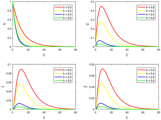
Figure 3. The relationship diagrams between the media intensity h and $s\left(t\right)$, $e\left(t\right)$, $i\left(t\right)$ and $f\left(t\right)$, respectively.

This indicates that increasing the intensity of media broadcasting is also an effective way to control the spread of the disease.

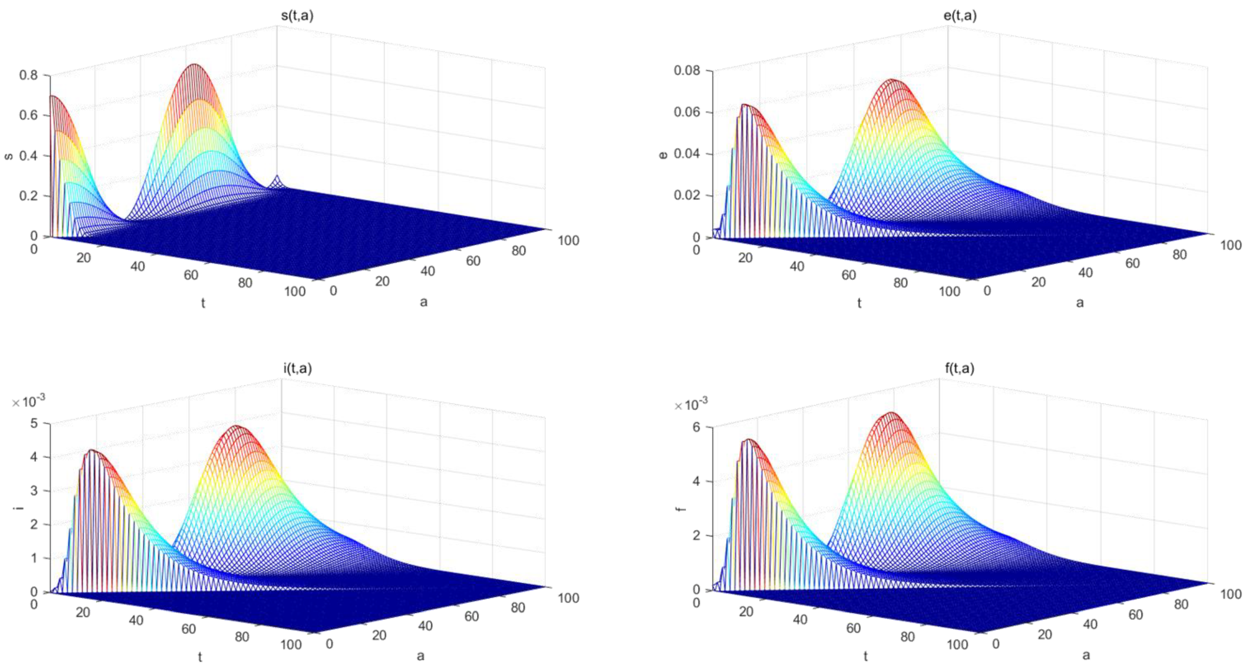
To obtain a numerical solution for system (2), the following initial age distribution is assumed:

$$s_0=0.7{\left(cos\left(0.05a\right)\right)}^2,e_0=0.004{\left(cos\left(0.05a\right)\right)}^2,$$

$$i_0=0.00004{\left(cos\left(0.05a\right)\right)}^2,f_0=0.0002{\left(cos\left(0.05a\right)\right)}^2.$$

From Figure 4, we can see that young people and the elderly are more affected by the disease, which is related to their wide range of activities, more contacts, and physical conditions.

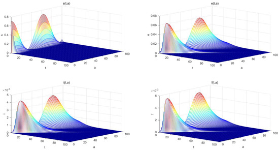
Figure 4. Plots of $s\left(t\right),e\left(t\right),i\left(t\right)$ and $f\left(t\right)$ versus age a and time t.

6. Conclusions

This paper investigates the SEIAR infectious disease model in which three main factors—the media effect, vaccination, and age structure—are considered, and the stability of the model is analyzed.

Firstly, it can be seen from the expression of $R_0$ that strengthening media propaganda can lead more people to transition from the exposed class to the recovered class through medication or other means, reducing the density of infectives and thus reducing the further spread of the epidemic. In particular, if $p=1$ in the expression of $R_0$, that is,

$$R_0={\int }_0^{a^{+}}\tilde{\beta }\left(a\right)\left\{{\int }_0^a\theta \left(\tau \right)e^{-{\int }_{\tau }^a\left[{\gamma }_1\left(s\right)+c\left(s\right)\right]ds}{\int }_0^{\tau }z\left(\xi \right)s^0\left(\xi \right)e^{-{\int }_{\xi }^{\tau }[\theta \left(s\right)+\phi \left(s\right)]ds}d\xi d\tau \right\}da,$$

it can be seen that the infectious disease can disappear more quickly in the absence of asymptomatic infections.

Secondly, vaccines stimulate the body to produce antibodies and immune cells to form immunity; the higher the success vaccination rate $\rho \left(a\right)$, the fewer the susceptible people in the population, and the easier it is to cut off the virus transmission chain (see Figure 1), thereby suppressing the spread of the epidemic.

Finally, age is not only an important factor for population growth patterns and the prevalence of infectious diseases but also has a certain impact on fertility rates, mortality rates, infection rates, and recovery rates. Therefore, applying an age-structured model to investigate the transmission dynamics of specific infectious diseases aligns with real-world scenarios.

However, this paper does not take into account the situation wherein vaccination becomes ineffective after a period of time or the infection process has a certain time lag. Future research will continue to discuss these issues.

References

- Ma, Z.E.; Zhou, Y.C.; Wang, W.D.; Jin, Z. Mathematical Modeling and Research on Infectious Disease Dynamics; Science Press: Beijing, China, 2004. (In Chinese) [Google Scholar]
- Kermack, O.W.; McKendrick, A.G. A contribution to the mathematical theory of epidemics. Proc. R. Soc. Lond. Ser. A 1927, 115, 700–721. [Google Scholar]
- Liu, R.S.; Wu, J.H.; Zhu, H.P. Media/psychological impact on multiple outbreaks of emerging infectious diseases. Comput. Math. Methods Med. 2007, 8, 153–164. [Google Scholar] [CrossRef]
- Tian, C.; Liu, Z.; Ruan, S.G. Asymptotic and transient dynamics of SEIR epidemic models on weighted networks. Eur. J. Appl. Math. 2023, 34, 238–261. [Google Scholar] [CrossRef]
- Wang, Q.; Xiang, K.N.; Zhu, C.H.; Zou, L. Stochastic SEIR epidemic models with virus mutation and logistic growth of susceptible populations. Math. Comput. Simulat. 2023, 212, 289–309. [Google Scholar] [CrossRef]
- Robinson, M.; Stilianakis, N.I. A model for the emergence of drug resistance in the presence of asymptomatic infections. Math. Biosci. 2013, 243, 163–177. [Google Scholar] [CrossRef] [PubMed]
- Grunnill, M. An exploration of the role of asymptomatic infections in the epidemiology of dengue viruses through susceptible, asymptomatic, infected and recovered (SAIR) models. J. Theor. Biol. 2018, 439, 195–204. [Google Scholar] [CrossRef]
- Aguilar, J.B.; Gutierrez, J.B. An epidemiological model of Malaria accounting for asymptomatic carriers. Bull Math. Biol. 2020, 82, 42. [Google Scholar] [CrossRef] [PubMed]
- Li, X.Z.; Gupur, G.; Zhu, G.T. Threshold and stability results for an age-structured SEIR epidemic model. Comput. Math. Appl. 2001, 42, 883–907. [Google Scholar] [CrossRef]
- Kar, T.K.; Nandi, S.K.; Jana, S.; Mandal, M. Stability and bifurcation analysis of an epidemic model with the effect of media. Chaos Soliton. Fract. 2019, 120, 188–199. [Google Scholar] [CrossRef]
- Xing, W.; Gao, J.F.; Yan, Q.S.; Zhou, Q.H.; Yang, Z.H. Qualitative analysis of an SEIS epidemic model affected by media reports. J. Northwest Univ. (Nat. Sci. Ed.) 2018, 48, 639–643. [Google Scholar]
- Greenhalgh, D. Analytical threshold and stability results on age-structured epidemic models with vaccination. Theor. Pop. Biol. 1988, 33, 266–290. [Google Scholar] [CrossRef] [PubMed]
- Greenhalgh, D. Threshold and stability results for an epidemic model with an age-structured meeting rate. IMA J. Math. Appl. Med. Biol. 1988, 5, 81–100. [Google Scholar] [CrossRef] [PubMed]
- Boots, M.; Greenman, J.; Ross, D.; Norman, R.; Hails, R.; Sait, S. The population dynamical implications of covert infections in host-microparasite interactions. J. Anim. Ecol. 2003, 72, 1064–1072. [Google Scholar] [CrossRef]
- Inaba, H. Mathematical analysis of an age-structured SIR epidemic model with vertical transmission. Discret. Contin. Dyn. Syst.—B. 2006, 6, 69–96. [Google Scholar] [CrossRef]
- Zaman, G.; Khan, A. Dynamical aspects of an age-structured SIR endemic model. Comput. Math. Appl. 2016, 72, 1690–1702. [Google Scholar] [CrossRef]
- Inaba, H. Age-Structured Population Dynamics in Demography and Epidemiology; Springer: Singapore, 2017. [Google Scholar]
- Kang, H.; Ruan, S.G.; Huang, Q.M. Periodic solutions of an age-structured epidemic model with periodic infection rate. Commun. Pure Appl. Anal. 2020, 19, 4955–4972. [Google Scholar] [CrossRef]
- Kang, H.; Ruan, S.G. Mathematical analysis on an age-structured SIS epidemic model with nonlocal diffusion. J. Math. Biol. 2021, 83, 5. [Google Scholar] [CrossRef]
- Huang, J.C.; Kang, H.; Lu, M.; Ruan, S.G.; Zhuo, W.T. Stability analysis of an age-structured epidemic model with vaccin ation and standard incidence rate. Nonlinear Anal. Real World Appl. 2022, 66, 103525. [Google Scholar] [CrossRef]
- Yu, Y.; Tan, Y.S.; Tang, S.Y. Stability analysis of the COVID-19 model with age structure under media effect. Comput. Appl. Math. 2023, 42, 204. [Google Scholar] [CrossRef]
- Yang, J.Y.; Zhou, M.; Feng, Z.S. Evaluation of age-structured vaccination strategies forcurbing the disease spread. J. Math. Biol. 2024, 88, 63. [Google Scholar] [CrossRef]
- Nabti, A.; Djilali, S.; Belghit, M. Dynamics of a double age-structured SEIRI epidemic model. Acta Appl. Math. 2025, 196, 9. [Google Scholar] [CrossRef]
Disclaimer/Publisher’s Note: The statements, opinions and data contained in all publications are solely those of the individual author(s) and contributor(s) and not of MDPI and/or the editor(s). MDPI and/or the editor(s) disclaim responsibility for any injury to people or property resulting from any ideas, methods, instructions or products referred to in the content. |
© 2025 by the authors. Licensee MDPI, Basel, Switzerland. This article is an open access article distributed under the terms and conditions of the Creative Commons Attribution (CC BY) license (https://creativecommons.org/licenses/by/4.0/).