Abstract
Neutral transmission line models are essential for analyzing stability and periodicity in systems influenced by nonlinear and delayed dynamics, particularly in modern smart grids. This study utilizes Krasnoselskii’s fixed-point theorem to establish sufficient conditions for the existence and asymptotic stability of periodic solutions, eliminating the need for differentiability in delay terms and coefficients. The results extend existing findings and are validated through a single test example, demonstrating the theoretical applicability of the proposed approach. These findings provide a mathematical framework for understanding the behavior of power distribution systems under nonlinear and delayed influences.
MSC:
34K13; 34A34; 34K30; 34L30
1. Introduction
Delay differential equations (DDEs) have emerged as indispensable tools for modeling complex dynamic systems influenced by delays, nonlinearities, and periodic behaviors. Their applications span a wide range of disciplines, including population dynamics, mechanical systems, and electrical circuits. Foundational studies, such as those by Burton [1] and Kuang [2], have laid the theoretical groundwork, exploring key properties like stability, positivity, and periodicity of solutions. These studies underscore the importance of DDEs in addressing intricate dynamical phenomena that arise in real-world systems. In addition, comprehensive discussions and significant advancements in these topics are documented across numerous studies [3,4,5,6,7,8,9,10,11,12,13,14,15,16,17,18,19,20,21,22,23,24].
The phenomenon of delay in dynamic systems is often associated with memory effects and hereditary properties, which have been mathematically described using integro-differential equations (IDEs). The foundational work of Vito Volterra [25,26,27,28,29] established the principles of hereditary systems, demonstrating how past states influence future evolution through integral formulations. These principles have significantly influenced the development of delay differential equations (DDEs), which serve as a more explicit representation of delayed interactions in various applications. By incorporating memory effects, IDEs and DDEs provide a rigorous mathematical framework for modeling real-world systems where delays play a critical role, such as energy transmission networks and biological systems.
Neutral transmission line models, a specific application of DDEs, are critical for analyzing the stability and periodicity of systems characterized by nonlinear and delayed dynamics. Their relevance has grown significantly in the context of modern smart grids, where the integration of renewable energy sources, variable loads, and communication delays presents unique challenges to stability and efficiency. Recent studies have established criteria for periodicity and stability in simplified and generalized neutral differential equation frameworks [30,31,32]. Notably, Ding and Li [31] leveraged Krasnoselskii’s fixed-point theorem to demonstrate periodic solutions in simplified models, while Mansouri et al. [32] extended these results to accommodate more complex dynamics involving variable delays and nonlinearities.
Despite these advancements, existing approaches are often constrained by assumptions such as the differentiability of delay terms and coefficients, which limit their applicability to real-world systems. In modern smart grids, such assumptions fail to capture the nondifferentiable dynamics introduced by renewable energy integration, time-varying power demands, and communication delays [33,34,35,36,37]. Addressing these gaps requires a more robust and flexible mathematical framework capable of capturing the interplay between nonlinear, delayed, and periodic behaviors.
This study aims to bridge this gap by exploring a more comprehensive class of nonlinear neutral transmission line models, removing the need for differentiability in delay terms and coefficients. By leveraging Krasnoselskii’s fixed-point theorem, this work introduces novel sufficient conditions for the existence and asymptotic stability of periodic solutions in the space . The derived results not only extend theoretical insights but also demonstrate practical relevance in optimizing power distribution within smart grids. The considered problem is given by
where a, b, and are positive -periodic continuous functions with ; q and p are -periodic continuous functions; is a continuous function; and is a locally Lipschitz continuous function, i.e., for , there is such that
A notable application of this research lies in addressing critical challenges in smart grid optimization. Renewable energy sources, such as solar and wind power, introduce periodic and nonlinear power variations that complicate grid stability. Additionally, power transmission delays, communication inefficiencies, and variable load conditions demand advanced analytical tools to maintain grid reliability and efficiency. The proposed model captures these complexities by incorporating nonlinear, delayed, and periodic dynamics, enabling precise analysis and control of voltage behavior. Furthermore, this approach aligns with contemporary advancements in machine learning and decentralized control, which further enhance grid performance and resilience [38,39].
Through theoretical analysis and practical examples, this work advances the mathematical modeling of nonlinear systems while providing actionable solutions to the pressing challenges of modern power systems. These findings pave the way for improved stability, efficiency, and resilience in smart grid operations, addressing the dynamic needs of contemporary energy networks.
To provide a clear roadmap for the reader, the remainder of this paper is structured as follows: In Section 2, we establish the existence of periodic solutions using fixed-point methods. Section 3 presents conditions for asymptotic stability, ensuring long-term system behavior remains predictable. In Section 4, we apply our theoretical findings to smart grid optimization, demonstrating their relevance in real-world power distribution challenges. Finally, Section 5 concludes this paper with a summary of our contributions and potential future research directions.
2. Existence of Periodic Solutions
Let be the set of all continuous functions . is equipped with the supremum norm in a period interval.
The following two lemmas will be applied in this work.
Lemma 1.
For , the differential equation admits a unique ϖ-periodic solution
where
Proof.
The proof can be found in ODE books (see for example, [4]). □
Lemma 2
(Krasnoselskii’s fixed point [40]). Let Ω be a closed bounded convex nonempty subset of a Banach space . Suppose that and map Ω into such that
- (i)
- implies ;
- (ii)
- is compact and continuous;
- (iii)
- is a contraction mapping.
Then, there is with .
In this section, by using Lemmas 1 and 2, we demonstrate the existence of -periodic solutions of (1).
Theorem 1.
Suppose that there exist and such that
and
Then, (1) admits a ϖ-periodic solution.
Proof.
From (3), we have
Let
which is a closed bounded convex set of .
For all , we rewrite (1) as
By applying Lemma 1, we obtain
Then,
Define Mappings and by
and
To demonstrate that (1) admits a -periodic solution, we shall make sure that and satisfy the assumptions of Lemma 2. For all , we have , and , . Now, let us discuss . We have
and
Therefore, . Meanwhile, we get
and
So,
and
Therefore,
by (4). Consequently, .
For all , . On the other hand, we have
Thus,
Therefore, there is a constant such that . From the Ascoli–Arzela theorem, for all of the sequence of , there is a subsequence of , such that as . Hence, is contained in a compact set. So, is a compact mapping.
Assume that , , . Then, as , and we obtain
Thus,
when as and for uniformly. And since is continuous, . Consequently, is continuous.
Now, for all , we have
Then,
Therefore, is a contraction mapping.
Thus, the assumptions of Lemma 2 are satisfied. Hence, there is a , such that . It is a -periodic solution for (1). □
3. Asymptotic Stability
We study the asymptotic stability of periodic solutions in this section. Let be a periodic solution of (1). For , (1) is transformed to
Clearly, (6) admits the zero solution. To demonstrate that the zero solution of (6) is asymptotically stable, we apply Krasnoselskii’s fixed-point theorem. Let be the Banach space of bounded continuous functions with the supremum norm and , . Moreover, for a given initial function , denote the norm of by .
Definition 1
([1]). The zero solution of (6) is asymptotically stable if it is Lyapunov-stable and if there exists a for any such that implies as .
Theorem 2.
Suppose that all assumptions of Theorem 1 are satisfied and that Ψ satisfies the locally Lipschitz condition. Also, assume that
and that there is such that
and
Then, the solution of (6) is .
Proof.
From (9), we obtain
There is a unique solution of (6) for the given initial function . Let
which is a closed convex bounded subset of . Now, we rewrite (6) as
Then,
Let , , and
For all , define the Mappings and by
(i) For all , and , as . Then,
and
Therefore, . We have
and
Then,
and
Thus,
By using Condition (10), we obtain . Hence, we continue with .
(ii) For all , , we have , and
We can see that is bounded for all and that is a relatively compact subset of . Hence, is compact.
Let , , as . Then, uniformly for as . Since
and is continuous, as , and is continuous.
(iii) For all , we have
Then,
Therefore, is a contraction mapping.
Consequently, there is a such that by applying Krasnoselskii’s fixed-point theorem. Hence, is a solution for (6). Since the solution through for the equation is unique, the solution as . □
When in Theorem 1 and Q in Theorem 2 exist, and satisfy the locally Lipschitz condition. Thus, there are constants such that
and
Since satisfies
then
that is,
Then, there clearly exists a for each such that for all if . Thus, we obtain the next theorem.
Theorem 3.
Suppose that and satisfy
Then, the zero solution for (6) is stable.
4. Application in Smart Grid Optimization
In this section, we explore the application of the modified model (1) to optimize the power distribution in smart grids. A smart grid is an advanced electrical grid system that integrates digital communication, automation, and modern control technologies to improve the efficiency, reliability, and sustainability of electricity production, distribution, and consumption. It enables two-way communication between power providers and consumers, allowing for real-time monitoring, demand response, and better integration of renewable energy sources. Modern smart grids face significant challenges due to the following:
- Variability in Renewable Energy Sources: Solar and wind power introduce periodic and nonlinear fluctuations in energy supply [34,37].
- Delays in Power Transmission and Communication: Signal transmission and control delays impact the stability of power distribution [33,35].
- Dynamic Load Demand: Fluctuations in electricity consumption require advanced models to maintain stability and efficiency [36].
4.1. Problem Statement
The findings in Section 2 and Section 3 provide a mathematical foundation for addressing these challenges. Specifically, the Existence of Periodic Solutions: Theorem 1 establishes sufficient conditions for periodic solutions in nonlinear neutral transmission line models. Traditional power system models often assume differentiability and linearity, which do not accurately capture the real-world behavior of smart grids. This directly applies to smart grids where voltage variations follow periodic patterns due to renewable energy sources [38,39]. Thus, there is a need for a robust mathematical framework that can address the following:
- Periodic and nonlinear variations in voltage and power flow.
- The impact of transmission delays on grid stability.
- The long-term asymptotic behavior of voltage fluctuations in the presence of nonlinearities.
4.2. Application of Theoretical Results
Equation (1) can address these challenges by capturing the essential dynamics of power distribution networks, where
- represents the voltage at a node in the network.
- models the periodic power input from renewable sources.
- accounts for delays due to transmission distances.
- and describe nonlinear load characteristics.
Using Equation (1), the voltage dynamics at each node can be modeled, considering the following:
- The nonlinear behavior of loads and power sources.
- Delayed feedback due to communication or signal propagation.
- Periodic variations in power generation and consumption.
The periodicity conditions in Theorem 1 ensure that under appropriate parameter constraints, the voltage will exhibit stable periodic behavior, avoiding instabilities in the grid.
4.3. Simulation of Voltage Dynamics
For the simulation of Model (1), the following parameters and functions were defined:
- T: Period of the system, .
- : Delay term, defined as .
- : Periodic coefficient, defined as .
- : Periodic coefficient, defined as .
- : Periodic power input, defined as .
- : Periodic coefficient, defined as .
- : Nonlinear function, defined as .
- : Nonlinear function, defined as .
These parameters and functions capture the nonlinear, delayed, and periodic behaviors relevant to the dynamics of voltage in a smart grid environment. The simulation of Model (1) was performed to analyze the voltage dynamics () over time. Figure 1 illustrates the result of the simulation, showing the periodic behavior.
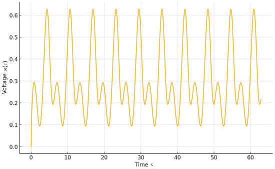
Figure 1.
Simulation of neutral transmission line model (1): voltage dynamics ().
5. Conclusions
In this paper, we developed new sufficient conditions for the existence and asymptotic stability of periodic solutions in nonlinear neutral transmission line models using Krasnoselskii’s fixed-point theorem. By removing differentiability assumptions on delay terms and coefficients, our results extend existing theoretical studies in the field. A test example was presented to illustrate the applicability of the proposed conditions.
Our findings contribute to the theoretical understanding of nonlinear neutral systems, particularly in the context of smart grid stability. However, additional research is needed to explore broader applications and validate the theoretical results with real-world data. Future work could consider numerical simulations, experimental validation, and extensions to more complex models incorporating stochastic effects or distributed parameter systems.
Author Contributions
Writing—original draft preparation, A.A. and M.B.M.; writing—review and editing, M.B.M., I.-L.P., H.S., F.H.D., Y.A.M. and T.S.H. All authors have read and agreed to the published version of the manuscript.
Funding
This research was funded by the Scientific Research Deanship at University of Ha’il, Saudi Arabia, through project number RG-24 161.
Data Availability Statement
Data are contained within the article.
Acknowledgments
This research was funded by the Scientific Research Deanship at University of Ha’il, Saudi Arabia, through project number RG-24 161.
Conflicts of Interest
The authors declare no conflicts of interest.
References
- Burton, T.A. Stability by Fixed Point Theory for Functional Differential Equations; Dover Publications: New York, NY, USA, 2006. [Google Scholar]
- Kuang, Y. Delay Differential Equations with Application in Population Dynamics; Academic Press: New York, NY, USA, 1993. [Google Scholar]
- Ardjouni, A.; Djoudi, A. Periodic solutions in totally nonlinear dynamic equations with functional delay on a time scale. Rend. Del Semin. Mat. Della Univ. Torino 2010, 68, 349–359. [Google Scholar]
- Burton, T.A. Liapunov functionals, fixed points and stability by Krasnoselskii’s theorem. Nonlinear Stud. 2002, 9, 181–190. [Google Scholar]
- Candan, T. Existence of positive periodic solutions of first-order neutral differential equations. Math. Methods Appl. Sci. 2017, 40, 205–209. [Google Scholar] [CrossRef]
- Candan, T. Existence of positive periodic solutions of first-order neutral differential equations with variable coefficients. Appl. Math. Lett. 2016, 52, 142–148. [Google Scholar] [CrossRef]
- Cheng, Z.; Ren, J. Existence of positive periodic solution for variable-coefficient third-order differential equation with singularity. Math. Methods Appl. Sci. 2014, 37, 2281–2289. [Google Scholar] [CrossRef]
- Cheng, Z.; Xin, Y. Multiplicity Results for variable-coefficient singular third-order differential equation with a parameter. Abstr. Appl. Anal. 2014, 2014, 527162. [Google Scholar] [CrossRef]
- Chen, F.D. Positive periodic solutions of neutral Lotka-Volterra system with feedback control. Appl. Math. Comput. 2005, 162, 1279–1302. [Google Scholar] [CrossRef]
- Chen, F.D.; Shi, J.L. Periodicity in a nonlinear predator-prey system with state dependent delays. Acta Math. Appl. Sin. Engl. Ser. 2005, 21, 49–60. [Google Scholar] [CrossRef]
- Fan, M.; Wang, K.; Wong, P.J.Y.; Agarwal, R.P. Periodicity and stability in periodic n-species Lotka-Volterra competition system with feedback controls and deviating arguments. Acta Math. Appl. Sin. Engl. Ser. 2003, 19, 801–822. [Google Scholar] [CrossRef]
- Freedman, H.I.; Wu, J. Periodic solutions of single-species models with periodic delay. Siam J. Math. Anal. 1992, 23, 689–701. [Google Scholar] [CrossRef]
- Liu, Y.; Ge, W. Positive periodic solutions of nonlinear Duffing equations with delay and variable coefficients. Tamsui Oxf. J. Math. Sci. 2005, 20, 235–255. [Google Scholar]
- Li, W.G.; Shen, Z.H. An constructive proof of the existence theorem for periodic solutions of Duffing equations. Chin. Sci. Bull. 1997, 42, 1591–1595. [Google Scholar]
- Mesmouli, M.B.; Ardjouni, A.; Djoudi, A. Stability conditions for a mixed linear Levin–Nohel integrodifferential system. J. Integral Equations Appl. 2022, 34, 349–356. [Google Scholar] [CrossRef]
- Mesmouli, M.B.; Attiya, A.A.; Elmandouha, A.A.; Tchalla, A.M.J.; Hassan, T.S. Dichotomy Condition and Periodic Solutions for Two Nonlinear Neutral Systems. J. Funct. Spaces 2022, 2022, 6319312. [Google Scholar] [CrossRef]
- Mesmouli, M.B.; Ardjouni, A.; Saber, H. Asymptotic Behavior of Solutions in Nonlinear Neutral System with Two Volterra Terms. Mathematics 2023, 11, 2676. [Google Scholar] [CrossRef]
- Mesmouli, M.B.; Menaem, A.A.; Hassan, T.S. Effectiveness of matrix measure in finding periodic solutions for nonlinear systems of differential and integro-differential equations with delays. Aims Math. 2024, 9, 14274–14287. [Google Scholar]
- Mesmouli, M.B.; Ardjouni, A.; Djoudi, A. A study of the stability in neutral nonlinear differential equations with functional delay via fixed points, Facta Universitatis. Ser. Math. Inform. 2016, 31, 609–627. [Google Scholar]
- Wang, Q. Positive periodic solutions of neutral delay equations. Acta Math. Sin. (N.S.) 1996, 6, 789–795. (In Chinese) [Google Scholar]
- Wang, Y.; Lian, H.; Ge, W. Periodic solutions for a second order nonlinear functional differential equation. Appl. Math. 2007, 20, 110–115. [Google Scholar] [CrossRef]
- Yuan, Y.; Guo, Z. On the existence and stability of periodic solutions for a nonlinear neutral functional differential equation. Abstr. Appl. Anal. 2013, 2013, 175479. [Google Scholar] [CrossRef]
- Zeng, W. Almost periodic solutions for nonlinear Duffing equations. Acta Math. Sin. (N.S.) 1997, 13, 373–380. [Google Scholar]
- Zhang, G.; Cheng, S. Positive periodic solutions of non autonomous functional differential equations depending on a parameter. Abstr. Appl. Anal. 2002, 7, 279–286. [Google Scholar]
- Volterra, V. Theory of Functionals and of Integral and Integro-Differential Equations; Dover Publications: New York, NY, USA, 2005; p. 288. [Google Scholar]
- Volterra, V. Sur les équations intégro-différentielles et leurs applications. Acta Math. 1912, 35, 295–356. [Google Scholar]
- Tunc, C.; Tunc, O. On the qualitative behaviors of Volterra-Fredholm integro differential equations with multiple time–Varying delays. Arab. J. Basic Appl. Sci. 2024, 31, 440–453. [Google Scholar]
- Mahmoud, A.M.; Tunç, C. On the qualitative behaviors of stochastic delay integro-differential equations of second order. J. Inequalities Appl. 2024, 2024, 35. [Google Scholar]
- Taier, A.E.; Wu, R.; Iqbal, N. Boundary value problems of hybrid fractional integro-differential systems involving the conformable fractional derivative. Aims Math. 2023, 8, 26260–26274. [Google Scholar]
- Ardjouni, A.; Djoudi, A. Existence of periodic solutions for a second-order nonlinear neutral differential equation with variable delay. Palest. J. Math. 2014, 3, 191–197. [Google Scholar]
- Ding, L.; Li, Z. Periodicity and stability in neutral equations by Krasnoselskii’s fixed point theorem. Nonlinear Anal. Real World Appl. 2010, 11, 1220–1228. [Google Scholar]
- Mansouri, B.; Ardjouni, A.; Djoudi, A. Periodicity and stability in neutral nonlinear differential equations by Krasnoselskii’s fixed point theorem. Cubo Math. J. 2017, 19, 15–29. [Google Scholar]
- Al-Anbagi, I.; Erol-Kantarci, M.; Mouftah, H.T. Priority-and delay-aware medium access for wireless sensor networks in the smart grid. IEEE Syst. J. 2013, 8, 608–618. [Google Scholar]
- Kabalci, Y.; Kabalci, E. Modeling and analysis of a smart grid monitoring system for renewable energy sources. Sol. Energy 2017, 153, 262–275. [Google Scholar]
- Eltigani, D.; Masri, S. Challenges of integrating renewable energy sources to smart grids: A review. Renew. Sustain. Energy Rev. 2015, 52, 770–780. [Google Scholar]
- Kundur, P. Power System Stability and Control; McGraw-Hill: New York, NY, USA, 1994. [Google Scholar]
- Lund, H. Renewable Energy Systems: A Smart Energy Systems Approach to the Choice and Modeling of 100% Renewable Solutions; Academic Press: Cambridge, MA, USA, 2014. [Google Scholar]
- Samadi, P.; Mohsenian-Rad, H.; Schober, R.; Wong, V.W. Advanced demand side management for the future smart grid using mechanism design. IEEE Trans. Smart Grid 2012, 3, 1170–1180. [Google Scholar]
- Erseghe, T. Distributed Optimal power Flow Using ADMM. IEEE Trans. Power Syst. 2014, 29, 2370–2380. [Google Scholar]
- Smart, D.R. Fixed Points Theorems; Cambridge University Press: Cambridge, UK, 1980. [Google Scholar]
Disclaimer/Publisher’s Note: The statements, opinions and data contained in all publications are solely those of the individual author(s) and contributor(s) and not of MDPI and/or the editor(s). MDPI and/or the editor(s) disclaim responsibility for any injury to people or property resulting from any ideas, methods, instructions or products referred to in the content. |
© 2025 by the authors. Licensee MDPI, Basel, Switzerland. This article is an open access article distributed under the terms and conditions of the Creative Commons Attribution (CC BY) license (https://creativecommons.org/licenses/by/4.0/).