Bayesian and Non-Bayesian for Generalized Kavya–Manoharan Exponential Distribution Based on Progressive-Stress ALT Under Generalized Progressive Hybrid Censoring Scheme

Abstract

Accelerated life tests are vital in reliability studies, especially as new technologies create highly reliable products to meet market demand and competition. Progressive stress accelerated life test (PSALT) allows continual stress adjustments. For reliability and survival analysis in accelerated life studies, generalized progressive hybrid censoring (GPHC) is very important. The research on GPHC in PSALT models is lacking despite its growing importance. Binomial elimination and generalized progressive hybrid censoring augment PSALT in this investigation. This research examines PSALT under the Generalized Kavya–Manoharan exponential distribution based on the GPHC scheme. Using gamma prior, maximum likelihood, and Bayesian techniques, estimate model parameters. Squared error and entropy loss functions yield Bayesian estimators using informational priors in simulation and non-informative priors in application. Various censoring schemes are calculated using Monte Carlo simulation. The methodology is demonstrated using two real-world accelerated life test data sets.

1. Introduction

Progress in science and technology has resulted in the creation of exceptionally durable and intricate products, like silicone seals, computers, missiles, and LEDs. Reliability is crucial for sustaining product quality, leading firms to invest significantly in testing and design. Nevertheless, for exceptionally reliable goods, their prolonged lifespans frequently provide minimal or no failures during regular testing under typical conditions. Conventional life-testing methodologies encounter difficulties in managing such situations.

In conventional life testing and reliability trials, acquiring adequate failure data can be difficult, particularly for highly dependable items with extended lifespans. Under typical circumstances, assessments performed within restricted durations frequently provide fewer failures. Accelerated life testing (ALT) is frequently employed to tackle this issue. ALT exposes products to heightened stress conditions, including enhanced humidity, temperature, pressure, voltage, or vibration, to expedite breakdown occurrences. The resultant failure statistics are subsequently evaluated to assess the product’s lifespan characteristics under standard operating settings. ALT can be executed by multiple methodologies, including continual stress, step stress, and progressive stress techniques, as articulated by Nelson [1]. To tackle this difficulty, ALT is utilized, wherein items are exposed to elevated stress conditions (e.g., temperature, voltage) to precipitate premature failures. This allows producers to forecast product longevity under standard usage conditions. Alternative methods encompass the following:

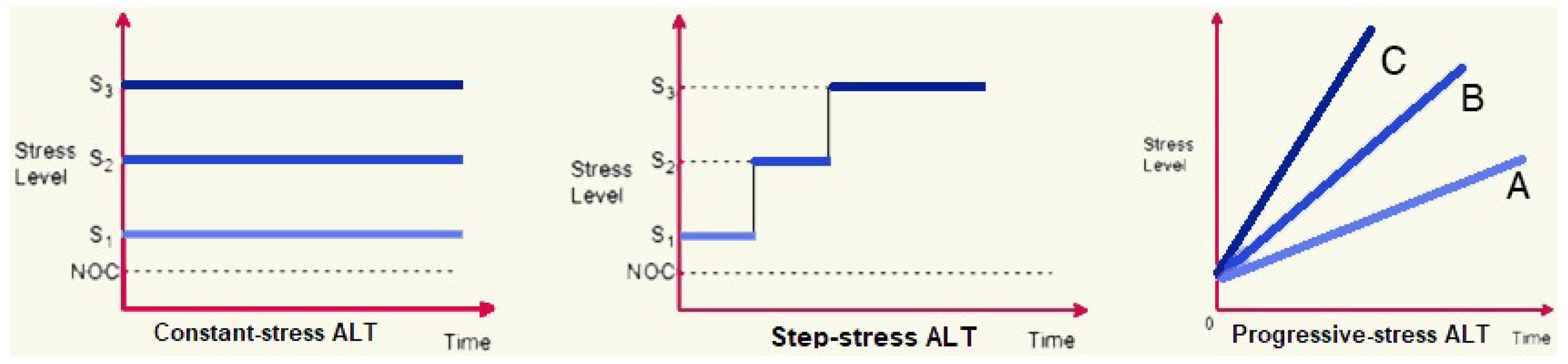
• Constant stress: applies a steady and unchanging high level of stress during the entire test.
• Step-stress: increases the stress level incrementally in distinct stages.
• Progressive stress: gradually raises the stress level in a continuous manner over time.

Refer to Nelson [1] for fundamental notions regarding ALT. ALT optimizes testing productivity, lowers costs, and improves product design by delivering critical failure data within reduced timescales. Figure 1 delineates the distinctions among ALT approaches.

1.1. Constant-Stress ALT

In constant-stress accelerated life testing, test units are exposed to a consistently high-stress environment until either all units fail or a specified stopping criterion is met. Notable contributions in this area are included in

Table 1. Key studies on constant-stress ALT.

Author(s)	Contribution
Kumar et al. [2]	Developed estimation procedures for the generalized inverse Lindley distribution.
Hakamipour et al. [3]	Proposed parameter estimation via the EM algorithm and optimized test designs under type-I progressive censoring.
Balakrishnan et al. [4]	Investigated optimal designs for one-shot devices and addressed model misspecification issues.
Abd El-Raheem et al. [5]	Conducted simulation and real data studies using the Pareto-IV distribution.
Sief et al. [6]	Applied maximum likelihood and Bayesian estimation to log-normal data under progressive type-I interval censoring.
El-Sherpieny et al. [7]	Studied statistical inference for bivariate distributions based on progressively censored samples with random removal.
Abd El-Raheem et al. [8]	Introduced a modified Kies exponential lifetime model with binomial removal, applied to transformer insulation.

.

1.2. Step-Stress ALT

Step-stress ALT entails the incremental augmentation of stress at predefined intervals or following a specified number of failures. This approach is extensively documented in the literature, with significant contributions including in

Table 2. Some studies on lifetime models with step-stress ALT model.

Author(s)	Contribution
Gouno et al. [9]	Developed optimal censoring strategies for lifetime distributions under progressive type-I censoring.
Balakrishnan et al. [10]	Presented methods for both point and interval estimation of parameters in life distribution models.
Mohie El-Din et al. [11]	Analyzed the power generalized Weibull distribution under progressive type-II censoring.
Alotaibi et al. [12]	Investigated the Kavya–Manoharan exponentiated Weibull model in the context of progressive censoring.
Alotaibi et al. [13]	Conducted statistical inference for competing risks under time censoring using the alpha power exponential distribution.

.

1.3. Progressive-Stress ALT

Progressive stress ALT has a distinctive methodology in contrast to constant and step-stress techniques by progressively escalating stress levels over time. An illustrative instance is the ramp stress test, characterized by a linear increase in stress. Researchers have investigated multiple facets of this approach, with significant contributions included in

Table 3. Key studies on progressive-stress models.

Author(s)	Contribution
Yin and Sheng [14]	Analyzed maximum likelihood estimation (MLE) procedures within exponential models under progressive-stress testing.
Bai and Cha [15]	Investigated optimal test plans and failure rate modeling in the context of progressive-stress scenarios.
Wang and Fei  [16]	Studied statistical inference for Weibull distributions applied to tampered failure rate models.
AL-Hussaini et al. [17]	Developed Bayesian prediction intervals for the half-logistic distribution using progressively type-II censored data under progressive-stress conditions.

.

These studies illustrate ALT’s efficacy in tackling issues associated with highly reliable goods, offering insights into statistical models, optimal test designs, and sophisticated failure analysis methodologies.

Censored data are frequently utilized in research about dependability and life testing. Investigators must collect data using censored samples due to considerations such as the preservation of operational experimental equipment for future utilization, the minimization of overall testing duration, and financial constraints. Time-censoring (type I) and failure-censoring (type II) are the two predominant censoring strategies employed in life-testing and reliability studies (see the work by Bain and Engelhardt for further details [18]). These approaches lack sufficient flexibility to permit the removal of units from the experiment at any time other than the final point.

The progressive type-II censoring scheme (PTII) is a commonly employed technique in reliability and survival analysis, frequently favored over the conventional type-II censoring scheme due to its versatility in practical applications, including industrial and medical research. In contrast to the traditional methodology, PTII allows for the extraction of functioning units throughout the experiment rather than at its completion [19]. In PTII, let m represent the number of units out of n that are designated to fail during a life test. A specified sequence $(R_1,R_2,\dots ,R_m)$ determines the number of units extracted following each failure. Upon the initial failure occurring at time $X_{1:m:n}$, $R_1$ remaining units are deleted arbitrarily. Likewise, following the second failure at $X_{2:m:n}$, $R_2$ supplementary units are extracted. The procedure persists until the m-th failure at $X_{m:m:n}$, at which point all $R_m$ remaining units are eliminated, therefore ending the test. This method has been thoroughly examined; nonetheless, it has a significant limitation: if the units exhibit great reliability, the time of the experiment may become unduly prolonged.

Kundu and Joarder [20] proposed the progressive hybrid censoring scheme to overcome this issue, wherein the test concludes at $min(T,X_{m:m:n})$, with T representing a preset maximum duration. Nonetheless, the progressive hybrid censoring scheme encounters difficulties when only a few failures transpire before T, resulting in constrained or inaccurate parameter estimates. To address these issues, Cho et al. [21] introduced the GPHC scheme (GPHCS). This technique guarantees a minimal occurrence of failures, hence enhancing the precision of parameter estimates. Under GPHCS, the number of failures and their respective lifespan are pre-established, optimizing test length and expense. 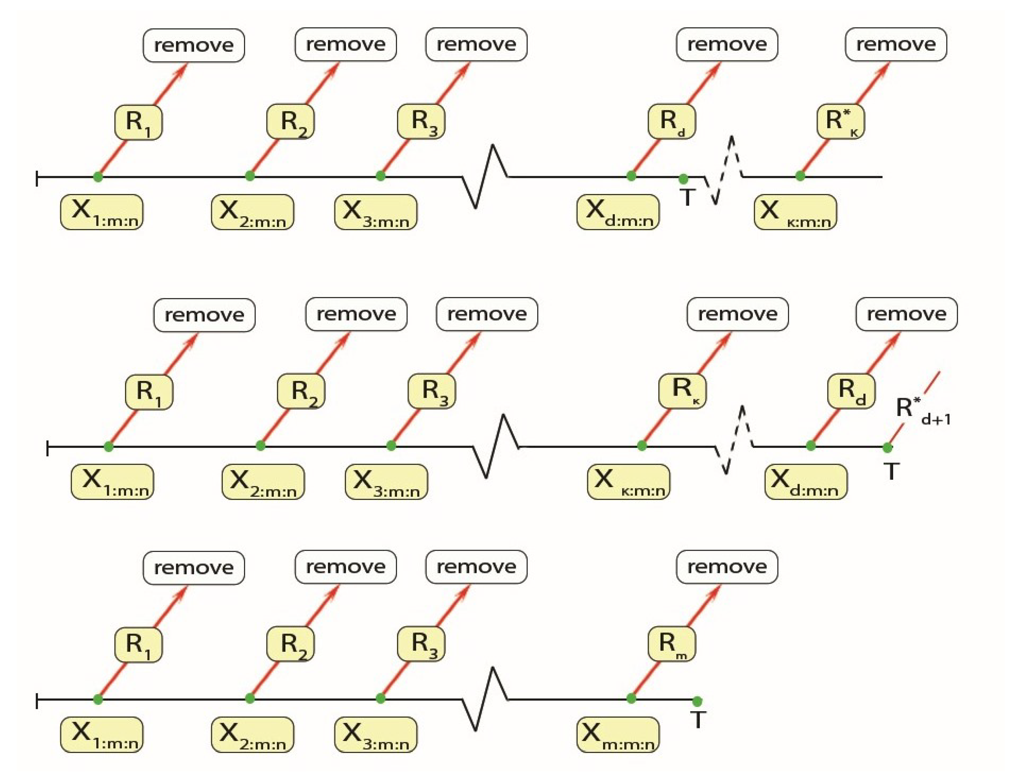The experiment finishes at $T^{*}=max\{X_{k:m:n},min\{X_{m:m:n},T\}\}$, with k, m, and $(R_1,\dots ,R_m)$ being predetermined, as referenced in [20]. The observations are classified into three categories:

• Case I: $X_{1:m:n},X_{2:m:n},\dots ,X_{k:m:n},$ if $T<X_{k:m:n}<X_{m:m:n}$,
• Case II: $X_{1:m:n},\dots ,X_{k:m:n},\dots ,X_{D:m:n},$ if $X_{k:m:n}<T<X_{m:m:n}$,
• Case III: $X_{1:m:n},\dots ,X_{k:m:n},\dots ,X_{m:m:n},$ if $X_{k:m:n}<X_{m:m:n}<T$,

Figure 2 illustrates a schematic illustration of the generalized progressive hybrid censoring scheme.

GPHCS was utilized by Koley and Kundu [22] to develop a new dialogue regarding censored samples within the context of conflicting hazard models. Maswadah [23] enhanced maximum likelihood estimation for the shape-scale family utilizing GPHCS. Salem et al. [24] presented the combined type II of GPHCS. Abdelwahab et al. [25] examined classical and Bayesian inference for lifespan distribution utilizing GPHCS. Mohie El-Din et al. [26] derived predictions of lives under GPHCS. Mahto et al. [27] formulated a partially observable competitive risk model inside the framework of GPHSC. Zhu derived reliability inference for the multi-component stress–strength model under GPHCS. Wang et al. [16] examined the reliance of competing risks on partially observed failure reasons derived from a bivariate distribution under GPHCS. Çetinkaya [28] examined the inference of P(X > Y) within the framework of GPHCS. Shi et al. [29] presented a reliability analysis of the J-out-of-N system under GPHCS.

Research on progressive-stress ALT is always advancing, integrating various statistical models and censoring methodologies. Abdel-Hamid and Al-Hussaini [30] integrated progressive stress with finite mixture distributions, Bayesian analysis, and progressive censoring for multiple lifespan distributions. Abdel-Hamid and Al-Hussaini [31] investigated inference for Weibull distributions in the context of PTII filtering. Recent studies employing progressive-stress ALT with censoring methodologies encompass the works of Mohie et al. [32], Zhuang [33], Mahto [34], Abushal [35], Ismail [36], Hussam [37], and Alotaibi [38].

The GPHCS has demonstrated its efficacy as a valuable instrument for studying censored data in ALTs, especially within models such as competing risks and step-stress models. Nonetheless, a notable deficiency is present in the implementation of GPHC under Progressive Stress ALT models, which entail incrementally escalating stress levels during the assessment. The majority of current research, including that by Wang et al. [39] and Pandey et al. [40], concentrates on constant or step-stress models, neglecting the complexity associated with progressive stress scenarios.

The present study seeks to address this deficiency by modifying and expanding the GPHC methodology for PSALT models. The objective is to deliver a more adaptable and precise analytical instrument capable of managing censored data resulting from incremental stress, thereby enhancing the accuracy of forecasts in progressive life-testing contexts. This study identifies a significant deficiency in the literature and facilitates the development of more accurate models for accelerated life testing.

2. Test Assumptions

2.1. Generalized Kavya–Manoharan Exponential Distribution

To provide more leeway for modeling lifetime data, the generalized Kavya–Manoharan exponential (GKME) distribution was created as an expansion of the exponential distribution. Developed by Mahran et al. [41], this distribution incorporates a shape parameter, $\alpha$, which, when coupled with the principal scale parameter $\lambda$, permits a more precise representation of actual data, particularly in cases where classical models are inadequate. There is a PDF for the GKME distribution, and it is found by

$$f(x;\alpha ,\lambda )={\displaystyle \frac{\alpha \lambda }{{(e-1)}^{\alpha }}}{e}^{-\lambda x+e^{-\lambda x}}{\left(e-e^{e^{-\lambda x}}\right)}^{\alpha -1};\alpha >0,\lambda >0,x\ge 0.$$

(1)

The cumulative distribution function (CDF) of the GKME distribution is given by

$$F(x;\alpha ,\lambda )={\displaystyle \frac{1}{{(e-1)}^{\alpha }}}{\left(e-e^{e^{-\lambda x}}\right)}^{\alpha };x\ge 0,$$

(2)

2.2. Assumption: Progressive-Stress ALT

• Lifetimes of units follow $GKME(\alpha ,\lambda )$.
• We have stress function $S\left(t\right)=\nu t$, $\nu >0$.
• The $S\left(t\right)$ depends upon t.
• We also have $\delta \left(t\right)={\displaystyle \frac{1}{{\theta }_1{\left[S\left(t\right)\right]}^{{\theta }_2}}}$, where ${\theta }_1,{\theta }_2>0$ and are to be estimated.
• Linear cumulative exposure model (LCEM) is considered for modeling the effect of stress change, for more details, see Nelson [1].

Under consideration of LCEM, the CDF under progressive-stress $S_i\left(t\right)$ is expressed as

$$G_i\left(t\right)=F_i(\Delta t),i=1,2,\dots ,s,$$

where $F_i$ denotes the CDF of the lifetime distribution at stress level i, $i=1,2,\dots ,s$, while s is the total number of progressive stress levels, and

$$\Delta t={\int }_0^t{\displaystyle \frac{dw}{{\delta }_i\left(w\right)}}={\displaystyle \frac{{\theta }_1{\nu }_i^{{\theta }_2}{t}^{{\theta }_2+1}}{{\theta }_2+1}},$$

where ${\delta }_i\left(w\right)={\displaystyle \frac{1}{{\theta }_1{\left[S_i\left(w\right)\right]}^{{\theta }_2}}}$ is the time-dependent degradation rate function associated with the i-th stress level.

Then, by setting the value of the scale parameter $\lambda =1$, we have the CDF for the i-th progressive stress given as

$$G_i(t;\Omega )={\displaystyle \frac{1}{{(e-1)}^{\alpha }}}{\left[e-e^{\left(e^{-{\displaystyle \frac{{\theta }_1{\nu }_i^{{\theta }_2}{t}^{{\theta }_2+1}}{{\theta }_2+1}}}\right)}\right]}^{\alpha };t>0,\alpha ,{\theta }_1,{\theta }_2>0,$$

(3)

where $\Omega$ is vector of parameter as $(\alpha ,{\theta }_1,{\theta }_2)$, and the corresponding PDF is given by

$$g_i(t;\Omega )={\displaystyle \frac{\alpha {\theta }_1{\nu }_i^{{\theta }_2}}{{(e-1)}^{\alpha }}}{t}^{{\theta }_2}{e}^{-{\displaystyle \frac{{\theta }_1{\nu }_i^{{\theta }_2}{t}^{{\theta }_2+1}}{{\theta }_2+1}}+e^{-{\displaystyle \frac{{\theta }_1{\nu }_i^{{\theta }_2}{t}^{{\theta }_2+1}}{{\theta }_2+1}}}}{\left[e-e^{\left(e^{-{\displaystyle \frac{{\theta }_1{\nu }_i^{{\theta }_2}{t}^{{\theta }_2+1}}{{\theta }_2+1}}}\right)}\right]}^{\alpha -1}.$$

(4)

2.3. Algorithm: GPHCS

• Input:
  • Distribution election: the GKME distribution is chosen for this study.
  • Number of units: n.
  • Predefined time: $T>0$.
  • Failure counts: k and m where $k<m\le n$.
  • Censoring plan: a sequence $(R_1,R_2,\dots ,R_m)$ such that $m+{\sum }_{i=1}^m{R}_i=n$.
• Procedure:

  (a)

  Deploy n units for life testing.

  (b)

  Simulate lifetimes based on the GKME distribution with CDF $F(x;\sigma )$, using PTII methodology [42].

  • Assign values for $\sigma$.
  • For given values of n, m, and $R_i$ ($i=1,2,\dots ,m$), generate a PTII sample:
    • Draw $v_1,v_2,\dots ,v_m$ as independent samples from a uniform $U(0,1)$ distribution.
    • Compute

      $${\tau }_i=v_i^{{\left(i+{\sum }_{l=m-i+1}^m{R}_l\right)}^{-1}},i=1,2,\dots ,m.$$
    • Calculate

      $$U_i=1-{\tau }_m{\tau }_{m-1}\dots {\tau }_{m-i+1},i=1,2,\dots ,m.$$
    • Invert the GKME distribution to determine

      $$X_{i:m:n}=F^{-1}(U_i;\sigma ),i=1,2,\dots ,m.$$
    • The resulting values $X_{1:m:n},X_{2:m:n},\dots ,X_{m:m:n}$ represent PTII order statistics from the GKME distribution.

  (c)

  Set the failure time threshold as

  $$T^{*}=max\{X_{k:m:n},min\{X_{m:m:n},T\}\}$$

  where

  $$T^{*}=\left\{\begin{array}{cc}T,\hfill & \mathrm{if}{X}_{k:m:n}<T<X_{m:m:n},\hfill \\ X_{k:m:n},\hfill & \mathrm{if}T<X_{k:m:n}<X_{m:m:n},\hfill \\ X_{m:m:n},\hfill & \mathrm{if}{X}_{k:m:n}<X_{m:m:n}<T.\hfill \end{array}\right.$$

  (d)

  Determine the number of failures for different cases:

  $$D=\left\{\begin{array}{cc}k,\delta =0\hfill & \mathrm{if}T\le X_{k:m:n}<X_{m:m:n},\hfill \\ d,\delta =1\hfill & \mathrm{if}{X}_{k:m:n}<T\le X_{m:m:n},\hfill \\ m,\delta =0\hfill & \mathrm{if}{X}_{k:m:n}<X_{m:m:n}<T.\hfill \end{array}\right.$$

  Here, $\delta$ is an indicator variable used to distinguish the termination mechanism of the test. It equals 1 when the experiment ends due to the pre-specified time T (i.e., time-censoring), and 0 when it ends due to the occurrence of m failures.
• Output: The observed failure times $X_{1:m:n},X_{2:m:n},\dots ,X_{d:m:n}$, where the following is true:

  (a)

  If $T<X_{k:m:n}<X_{m:m:n}$, then $d=k$.

  (b)

  If $X_{k:m:n}<T<X_{m:m:n}$, then d represents the number of failures before T.

  (c)

  If $X_{k:m:n}<X_{m:m:n}<T$, then $d=m$.

3. Estimation Methods

In this section, we utilize the maximum likelihood estimation method based on PSALT to estimate the model parameters $\alpha$, ${\theta }_1$, and ${\theta }_2$. A concise explanation of GPHCS under PSALT is provided. Consider s stress levels, where $n_i$ items are subjected to testing at each level, with $i=1,2,\dots ,s$. Additionally, the observed items, denoted as $m_i$, $k_i$, and $T_i$, for $i=1,2,\dots ,s$, follow predefined censoring schemes ${\mathcal{R}}_{i1},{\mathcal{R}}_{i2},\dots ,{\mathcal{R}}_{i{m}_i}$ at failure times $t_{1:m_i:n_i},t_{2:m_i:n_i},\dots ,t_{m_i:m_i:n_i}$, for $i=1,2,\dots ,s$.

During the first failure at the ith stress level, ${\mathcal{R}}_{i1}$ surviving units are removed from the experiment. Similarly, at the second failure in the ith stress level, ${\mathcal{R}}_{i2}$ surviving units are withdrawn from the remaining $(n_i-2-{\mathcal{R}}_{i1})$ units. Finally, at the $m_i$th failure, all the remaining units, calculated as ${\mathcal{R}}_{i{m}_i}=n_i-m_i-{\sum }_{j=1}^{m_i-1}{\mathcal{R}}_{ij}$, are withdrawn, bringing the experiment to an end. Refer to Figure 2 for illustration.

Let the observed GPHCS data under the progressive-stress level $S_i\left(t\right)$, for $i=1,2,\dots ,s$ be represented by $t_{ij}$. Here, $i=1,2,\dots ,s$ and $j=1,2,\dots ,m_i$. The corresponding likelihood function with vector parameter $\Omega$ is then expressed as follows:

$$L(\Omega )=\prod _{i=1}^s\left[C_i\prod _{j=1}^{D_i}{g}_i(t_{ij};\Omega ){\left(1-G_i(t_{ij};\Omega )\right)}^{R_{ij}}{\left(1-G_i(T_i;\Omega )\right)}^{{\delta }_i{R}_{T_i}^{*}}\right],$$

(5)

where $C_i$ is constant and does not depend on parameters $\Omega$, the $R_{T_i}^{*}$ can be define as $n_i-m_i-{\sum }_{j=1}^{D_i}{R}_{ij}$.

Using Equations (3) and (4) in (5), the likelihood function of the QXG distribution under GPHCS within the framework of the PSALT model is derived as

$$\begin{array}{cc}\hfill L(\Omega )=\prod _{i=1}^s& \left[C_i{\displaystyle \frac{{\alpha }^{D_i}{\theta }_1^{D_i}{\nu }_i^{D_i{\theta }_2}}{{(e-1)}^{\alpha D_i}}}{e}^{-{\displaystyle \frac{{\theta }_1{\nu }_i^{{\theta }_2}}{{\theta }_2+1}}{\sum }_{j=1}^{D_i}{t}_{ij}^{{\theta }_2+1}}\prod _{j=1}^{D_i}{e}^{e^{-{\displaystyle \frac{{\theta }_1{\nu }_i^{{\theta }_2}{t}_{ij}^{{\theta }_2+1}}{{\theta }_2+1}}}}{\left[e-e^{\left(e^{-{\displaystyle \frac{{\theta }_1{\nu }_i^{{\theta }_2}{t}_{ij}^{{\theta }_2+1}}{{\theta }_2+1}}}\right)}\right]}^{\alpha -1}\times \right.\hfill \\ & \left.{\left(1-{\displaystyle \frac{1}{{(e-1)}^{\alpha }}}{\left[e-e^{\left(e^{-{\displaystyle \frac{{\theta }_1{\nu }_i^{{\theta }_2}{t}_{ij}^{{\theta }_2+1}}{{\theta }_2+1}}}\right)}\right]}^{\alpha }\right)}^{R_{ij}}\times {\left(1-{\displaystyle \frac{1}{{(e-1)}^{\alpha }}}{\left[e-e^{\left(e^{-{\displaystyle \frac{{\theta }_1{\nu }_i^{{\theta }_2}{T}_i^{{\theta }_2+1}}{{\theta }_2+1}}}\right)}\right]}^{\alpha }\right)}^{{\delta }_i{R}_{T_i}^{*}}\right],\hfill \end{array}$$

(6)

hence, the log-likelihood function, excluding the constant term $C_i$, is expressed as

$$\begin{array}{cc}\hfill \mathsf{\ell }(\Omega )=& \sum _{i=1}^{s}ln{C}_i+\sum _{i=1}^s{D}_i\left(ln\alpha +ln{\theta }_1+{\theta }_{2}ln{\nu }_i-\alpha ln(e-1)\right)-\sum _{i=1}^s{\displaystyle \frac{{\theta }_1{\nu }_i^{{\theta }_2}}{{\theta }_2+1}}\sum _{j=1}^{D_i}{t}_{ij}^{{\theta }_2+1}+\sum _{i=1}^s\sum _{j=1}^{D_i}{e}^{-{\displaystyle \frac{{\theta }_1{\nu }_i^{{\theta }_2}{t}_{ij}^{{\theta }_2+1}}{{\theta }_2+1}}}+\hfill \\ & (\alpha -1)\sum _{i=1}^s\sum _{j=1}^{D_i}ln\left[e-e^{\left(e^{-{\displaystyle \frac{{\theta }_1{\nu }_i^{{\theta }_2}{t}_{ij}^{{\theta }_2+1}}{{\theta }_2+1}}}\right)}\right]+\sum _{i=1}^s\sum _{j=1}^{D_i}{R}_{ij}ln\left(1-{\displaystyle \frac{1}{{(e-1)}^{\alpha }}}{\left[e-e^{\left(e^{-{\displaystyle \frac{{\theta }_1{\nu }_i^{{\theta }_2}{t}_{ij}^{{\theta }_2+1}}{{\theta }_2+1}}}\right)}\right]}^{\alpha }\right)+\hfill \\ & \sum _{i=1}^s{\delta }_i{R}_{T_i}^{*}\left(1-{\displaystyle \frac{1}{{(e-1)}^{\alpha }}}{\left[e-e^{\left(e^{-{\displaystyle \frac{{\theta }_1{\nu }_i^{{\theta }_2}{T}_i^{{\theta }_2+1}}{{\theta }_2+1}}}\right)}\right]}^{\alpha }\right).\hfill \end{array}$$

(7)

3.1. Newton–Raphson Algorithm

The likelihood equations are obtained by taking the first partial derivatives of the log-likelihood function in (7) with respect to $\alpha$, ${\theta }_1$, and ${\theta }_2$, expressed as

$$\begin{array}{cc}\hfill {\displaystyle \frac{\partial \mathsf{\ell }(\Omega )}{\partial \alpha }}=& \sum _{i=1}^s{\displaystyle \frac{D_i}{\alpha }}-ln(e-1)-\sum _{i=1}^s\sum _{j=1}^{D_i}{R}_{ij}{\displaystyle \frac{\left(-{(e-1)}^{-\alpha }ln(e-1)+\frac{1}{{(e-1)}^{\alpha }}ln\left[e-e^{\left(e^{-\frac{{\theta }_1{\nu }_i^{{\theta }_2}{t}_{ij}^{{\theta }_2+1}}{{\theta }_2+1}}\right)}\right]\right){\left[e-e^{\left(e^{-\frac{{\theta }_1{\nu }_i^{{\theta }_2}{t}_{ij}^{{\theta }_2+1}}{{\theta }_2+1}}\right)}\right]}^{\alpha }}{1-\frac{1}{{(e-1)}^{\alpha }}{\left[e-e^{\left(e^{-\frac{{\theta }_1{\nu }_i^{{\theta }_2}{t}_{ij}^{{\theta }_2+1}}{{\theta }_2+1}}\right)}\right]}^{\alpha }}}\hfill \\ \hfill & +\sum _{i=1}^s\sum _{j=1}^{D_i}ln\left[e-e^{\left(e^{-{\displaystyle \frac{{\theta }_1{\nu }_i^{{\theta }_2}{t}_{ij}^{{\theta }_2+1}}{{\theta }_2+1}}}\right)}\right]+\sum _{i=1}^s{\delta }_i{R}_{T_i}^{*}{\displaystyle \frac{\left(-{(e-1)}^{-\alpha }ln(e-1)+\frac{1}{{(e-1)}^{\alpha }}ln\left[e-e^{\left(e^{-\frac{{\theta }_1{\nu }_i^{{\theta }_2}{T}_i^{{\theta }_2+1}}{{\theta }_2+1}}\right)}\right]\right){\left[e-e^{\left(e^{-\frac{{\theta }_1{\nu }_i^{{\theta }_2}{T}_i^{{\theta }_2+1}}{{\theta }_2+1}}\right)}\right]}^{\alpha }}{1-\frac{1}{{(e-1)}^{\alpha }}{\left[e-e^{\left(e^{-\frac{{\theta }_1{\nu }_i^{{\theta }_2}{T}_i^{{\theta }_2+1}}{{\theta }_2+1}}\right)}\right]}^{\alpha }}}.\hfill \end{array}$$

(8)

$$\begin{array}{cc}\hfill {\displaystyle \frac{\partial \mathsf{\ell }(\Omega )}{\partial {\theta }_1}}=& \sum _{i=1}^s{\displaystyle \frac{D_i}{{\theta }_1}}-\sum _{i=1}^s\sum _{j=1}^{D_i}{\displaystyle \frac{{\nu }_i^{{\theta }_2}{t}_{ij}^{{\theta }_2+1}}{{\theta }_2+1}}{e}^{-{\displaystyle \frac{{\theta }_1{\nu }_i^{{\theta }_2}{t}_{ij}^{{\theta }_2+1}}{{\theta }_2+1}}}+(\alpha -1)\sum _{i=1}^s\sum _{j=1}^{D_i}{\displaystyle \frac{A_i({\theta }_1,{\theta }_2,t_{ij})}{e-e^{\left(e^{-\frac{{\theta }_1{\nu }_i^{{\theta }_2}{t}_{ij}^{{\theta }_2+1}}{{\theta }_2+1}}\right)}}}-\sum _{i=1}^s{\displaystyle \frac{{\nu }_i^{{\theta }_2}}{{\theta }_2+1}}\sum _{j=1}^{D_i}{t}_{ij}^{{\theta }_2+1}\hfill \\ \hfill & +{\displaystyle \frac{\alpha }{{(e-1)}^{\alpha }}}\sum _{i=1}^s\sum _{j=1}^{D_i}{R}_{ij}{\displaystyle \frac{A_i({\theta }_1,{\theta }_2,t_{ij}){\left[e-e^{\left(e^{-\frac{{\theta }_1{\nu }_i^{{\theta }_2}{t}_{ij}^{{\theta }_2+1}}{{\theta }_2+1}}\right)}\right]}^{\alpha -1}}{1-\frac{1}{{(e-1)}^{\alpha }}{\left[e-e^{\left(e^{-\frac{{\theta }_1{\nu }_i^{{\theta }_2}{t}_{ij}^{{\theta }_2+1}}{{\theta }_2+1}}\right)}\right]}^{\alpha }}}+\sum _{i=1}^s{\delta }_i{R}_{T_i}^{*}{\displaystyle \frac{A_i({\theta }_1,{\theta }_2,T_i){\left[e-e^{\left(e^{-\frac{{\theta }_1{\nu }_i^{{\theta }_2}{T}_i^{{\theta }_2+1}}{{\theta }_2+1}}\right)}\right]}^{\alpha -1}}{1-\frac{1}{{(e-1)}^{\alpha }}{\left[e-e^{\left(e^{-\frac{{\theta }_1{\nu }_i^{{\theta }_2}{T}_i^{{\theta }_2+1}}{{\theta }_2+1}}\right)}\right]}^{\alpha }}}.\hfill \end{array}$$

(9)

and

$$\begin{array}{cc}\hfill {\displaystyle \frac{\partial \mathsf{\ell }(\Omega )}{\partial {\theta }_2}}=& \sum _{i=1}^s{D}_{i}ln{\nu }_i-\sum _{i=1}^s\sum _{j=1}^{D_i}{B}_i({\theta }_1,{\theta }_2,t_{ij})e^{-{\displaystyle \frac{{\theta }_1{\nu }_i^{{\theta }_2}{t}_{ij}^{{\theta }_2+1}}{{\theta }_2+1}}}+(\alpha -1)\sum _{i=1}^s\sum _{j=1}^{D_i}{\displaystyle \frac{B_i({\theta }_1,{\theta }_2,t_{ij})W_i({\theta }_1,{\theta }_2,t)}{e-e^{\left(e^{-\frac{{\theta }_1{\nu }_i^{{\theta }_2}{t}_{ij}^{{\theta }_2+1}}{{\theta }_2+1}}\right)}}}\hfill \\ \hfill & -\sum _{i=1}^s\sum _{j=1}^{D_i}{B}_i({\theta }_1,{\theta }_2,t_{ij})-{\displaystyle \frac{\alpha }{{(e-1)}^{\alpha }}}\sum _{i=1}^s\sum _{j=1}^{D_i}{R}_{ij}{\displaystyle \frac{B_i({\theta }_1,{\theta }_2,t_{ij})W_i({\theta }_1,{\theta }_2,t){\left[e-e^{\left(e^{-\frac{{\theta }_1{\nu }_i^{{\theta }_2}{t}_{ij}^{{\theta }_2+1}}{{\theta }_2+1}}\right)}\right]}^{\alpha -1}}{1-\frac{1}{{(e-1)}^{\alpha }}{\left[e-e^{\left(e^{-\frac{{\theta }_1{\nu }_i^{{\theta }_2}{t}_{ij}^{{\theta }_2+1}}{{\theta }_2+1}}\right)}\right]}^{\alpha }}}\hfill \\ \hfill & -{\displaystyle \frac{\alpha }{{(e-1)}^{\alpha }}}\sum _{i=1}^s\sum _{j=1}^{D_i}{R}_{ij}{\displaystyle \frac{B_i({\theta }_1,{\theta }_2,T_i)W_i({\theta }_1,{\theta }_2,T_i){\left[e-e^{\left(e^{-\frac{{\theta }_1{\nu }_i^{{\theta }_2}{T}_i^{{\theta }_2+1}}{{\theta }_2+1}}\right)}\right]}^{\alpha -1}}{1-\frac{1}{{(e-1)}^{\alpha }}{\left[e-e^{\left(e^{-\frac{{\theta }_1{\nu }_i^{{\theta }_2}{T}_i^{{\theta }_2+1}}{{\theta }_2+1}}\right)}\right]}^{\alpha }}}.\hfill \end{array}$$

(10)

where $A_i({\theta }_1,{\theta }_2,t)={\displaystyle \frac{{\nu }_i^{{\theta }_2}{t}_{ij}^{{\theta }_2+1}}{{\theta }_2+1}}{e}^{-{\displaystyle \frac{{\theta }_1{\nu }_i^{{\theta }_2}{t}^{{\theta }_2+1}}{{\theta }_2+1}}}{e}^{\left(e^{-{\displaystyle \frac{{\theta }_1{\nu }_i^{{\theta }_2}{t}^{{\theta }_2+1}}{{\theta }_2+1}}}\right)}$, $B_i({\theta }_1,{\theta }_2,t)={\theta }_1{\nu }_i^{{\theta }_2}{t}^{{\theta }_2+1}\left({\displaystyle \frac{({\theta }_2+1)ln{\nu }_i-1}{{({\theta }_2+1)}^2}}+{\displaystyle \frac{{\theta }_1{\nu }_i^{{\theta }_2}}{{\theta }_2+1}}lnt\right)$, and $W_i({\theta }_1,{\theta }_2,t)=e^{-{\displaystyle \frac{{\theta }_1{\nu }_i^{{\theta }_2}{t}_{ij}^{{\theta }_2+1}}{{\theta }_2+1}}}$ $e^{\left(e^{-{\displaystyle \frac{{\theta }_1{\nu }_i^{{\theta }_2}{t}_{ij}^{{\theta }_2+1}}{{\theta }_2+1}}}\right)}$.

The maximum likelihood estimates of the unknown parameters $\alpha$, ${\theta }_1$, and ${\theta }_2$ are determined by solving the three Equations (8)–(10) by setting them to zero. Since these equations are nonlinear, a numerical method is employed to compute the estimates, such as the Newton–Raphson (NR) algorithm. The NR algorithm begins with an initial estimate $({\alpha }^{\left(0\right)},{\theta }_1^{\left(0\right)},{\theta }_2^{\left(0\right)})$ and iteratively improves the estimates through the following update formula:

$${\Omega }^{\left(k\right)}={\Omega }^{(k-1)}-{\left[f^{\prime }\left({\Omega }^{(k-1)}\right)\right]}^{-1}f\left({\Omega }^{(k-1)}\right).$$

Here, $\Omega$ denotes the vector of unknown parameters, $f(\Omega )$ corresponds to the vector of first-order derivatives, and $f^{\prime }(\Omega )$ represents the Hessian matrix of second-order derivatives:

$$\Omega =\left[\begin{array}{c}\alpha \\ {\theta }_1\\ {\theta }_2\end{array}\right],f(\Omega )=\left[\begin{array}{c}{\displaystyle \frac{\partial \mathsf{\ell }(\Omega )}{\partial \alpha }}\\ {\displaystyle \frac{\partial \mathsf{\ell }(\Omega )}{\partial {\theta }_1}}\\ {\displaystyle \frac{\partial \mathsf{\ell }(\Omega )}{\partial {\theta }_2}}\end{array}\right],f^{\prime }(\Omega )=\left[\begin{array}{ccc}{\displaystyle \frac{{\partial }^2\mathsf{\ell }(\Omega )}{\partial {\alpha }^2}}& {\displaystyle \frac{{\partial }^2\mathsf{\ell }(\Omega )}{\partial \alpha \partial {\theta }_1}}& {\displaystyle \frac{{\partial }^2\mathsf{\ell }(\Omega )}{\partial \alpha \partial {\theta }_2}}\\ {\displaystyle \frac{{\partial }^2\mathsf{\ell }(\Omega )}{\partial {\theta }_1\partial \alpha }}& {\displaystyle \frac{{\partial }^2\mathsf{\ell }(\Omega )}{\partial {\theta }_1^2}}& {\displaystyle \frac{{\partial }^2\mathsf{\ell }(\Omega )}{\partial {\theta }_1\partial {\theta }_2}}\\ {\displaystyle \frac{{\partial }^2\mathsf{\ell }(\Omega )}{\partial {\theta }_2\partial \alpha }}& {\displaystyle \frac{{\partial }^2\mathsf{\ell }(\Omega )}{\partial {\theta }_2\partial {\theta }_1}}& {\displaystyle \frac{{\partial }^2\mathsf{\ell }(\Omega )}{\partial {\theta }_2^2}}\end{array}\right].$$

3.2. Asymptotic Confidence Interval

In this subsection, approximate confidence intervals for the parameters are derived using the asymptotic distribution of the MLEs of $\Omega =(\alpha ,{\theta }_1,{\theta }_2)$. The asymptotic distribution of the MLEs for $(\alpha ,{\theta }_1,{\theta }_2)$ is expressed as

$$((\widehat{\alpha }-\alpha ),({\widehat{\theta }}_1-{\theta }_1),({\widehat{\theta }}_2-{\theta }_2))\sim N(0,f^{\prime }{(\Omega )}^{-1}),$$

where $f^{\prime }{(\Omega )}_{ij}^{-1}$ represents the variance–covariance matrix of the parameters $\Omega$. The elements of the $3\times 3$ matrix $f^{\prime }{(\Omega )}^{-1}$ denoted as $f^{\prime }{(\Omega )}_{ij}$ for $i,j=1,2,3$ for $(\alpha ,{\theta }_1,{\theta }_2)$, can be approximated by $f^{\prime }{\left(\widehat{\Omega }\right)}_{ij}$. Accordingly, an approximate $100(1-p)\%$ confidence interval for the parameter $\Omega$ is given by

$${\widehat{\Omega }}_i\pm Z_{1-p/2}\sqrt{f^{\prime }{(\Omega )}_{ii}^{-1}},i=1,2,3,$$

where ${\widehat{\Omega }}_1\equiv \widehat{\alpha }$, ${\widehat{\Omega }}_2\equiv {\widehat{\theta }}_1$, and ${\widehat{\Omega }}_3\equiv {\widehat{\theta }}_2$.

The following section explores the incorporation of prior knowledge into the analysis to achieve improved results.

4. Bayesian Estimation

In this section, we introduce Bayesian estimates that address the GKME parameter uncertainty by considering a joint prior distribution formulated before collecting failure data. Utilizing prior knowledge in the analysis, the Bayesian approach proves valuable in reliability assessment. Through the squared error loss function (SELF) and entropy loss function (ELF), we derive Bayesian estimates (BEs) for the unidentified parameters $\lambda$ and $\omega$. These parameters are assumed to be independent and to adhere to gamma prior distributions as follows:

$$\left\{\begin{array}{c}{\pi }_1\left(\alpha \right)\propto {\alpha }^{q_1-1}{e}^{-w_1\alpha },\alpha >0,\\ {\pi }_2\left({\theta }_1\right)\propto {\theta }_1^{q_2-1}{e}^{-w_2{\theta }_1},{\theta }_1>0,\\ {\pi }_3\left({\theta }_2\right)\propto {\theta }_2^{q_3-1}{e}^{-w_3{\theta }_2},{\theta }_2>0.\end{array}\right.$$

(11)

It is presumed that all hyper-parameters $q_i$ and $w_i$ have positive values and are given.

The posterior distribution of parameters $\alpha , {\theta }_1$, and ${\theta }_2$, denoted as ${\pi }^{*}(\alpha ,{\theta }_1,{\theta }_2|\underset{\_}{\mathrm{x}})$, can be calculated by combining the likelihood function from Equation (6) with the prior distributions outlined in Equation (11).

$${\pi }^{*}\left(\Omega \mid \underset{\_}{\mathrm{x}}\right)={\displaystyle \frac{{\pi }_1\left(\alpha \right){\pi }_2\left({\theta }_1\right){\pi }_3\left({\theta }_2\right)L\left(x;\Omega \right)}{{\int }_0^{\infty }{\int }_0^{\infty }{\int }_0^{\infty }{\pi }_1\left(\alpha \right){\pi }_2\left({\theta }_1\right){\pi }_3\left({\theta }_2\right)L\left(x;\Omega \right)d\alpha d{\theta }_{1}d{\theta }_2}}.$$

(12)

Equation (12) represents the joint posterior distribution of the parameters $\alpha$, ${\theta }_1$, and ${\theta }_2$. It is derived by applying Bayes’ theorem, where the posterior is proportional to the product of the likelihood function (Equation (6)) and the prior distributions (Equation (11)), normalized by the marginal likelihood (i.e., the integral of the numerator over the parameter space).

The SELF is commonly used, as it is a symmetrical loss function that assigns the same penalties to both overestimation and underestimation. When an estimator $\widehat{\alpha }$, $\widehat{{\theta }_1}$ and $\widehat{{\theta }_2}$ is used to estimate the parameter $\alpha$, ${\theta }_1$, and ${\theta }_2$, the SELF is defined as $L\left(\alpha ,\widehat{\alpha }\right)=E{\left(\widehat{\alpha }-\alpha \right)}^2$, $L\left({\theta }_1,{\widehat{\theta }}_1\right)=E{\left({\widehat{\theta }}_1-{\theta }_1\right)}^2$, and $L\left({\theta }_2,{\widehat{\theta }}_2\right)=E{\left({\widehat{\theta }}_2-{\theta }_2\right)}^2$. Thus, the Bayesian estimation of any function involving $\alpha$, ${\theta }_1$, and ${\theta }_2$, such as $g\left(\alpha ,{\theta }_1,{\theta }_2\right)$ within the SELF framework, can be determined as

$${\widehat{g}}_{SELF}\left(\alpha ,{\theta }_1,{\theta }_2\mid \underset{\_}{\mathrm{x}}\right)=E_{\alpha ,{\theta }_1,{\theta }_2\mid \underset{\_}{\mathrm{x}}}\left(g\left(\alpha ,{\theta }_1,{\theta }_2\right)\right).$$

(13)

The ELF is the predominant choice for an asymmetric loss function, widely recognized as more comprehensive. The Bayesian estimate $g\left(\alpha ,{\theta }_1,{\theta }_2\right)$ under the ELF function can be calculated as follows:

$${\widehat{g}}_{ELF}\left(\alpha ,{\theta }_1,{\theta }_2\mid \mathrm{data}\right)=-{\displaystyle \frac{1}{\epsilon }}log\left[E\left(e^{-\epsilon g\left(\alpha ,{\theta }_1,{\theta }_2\right)}\mid \mathrm{data}\right)\right],\epsilon \ne 0,$$

(14)

4.1. Markov Chain Monte Carlo

Equation (13) offers an expectation that can be solved through various integrals, but obtaining these multiple integrals mathematically is not feasible. Hence, to generate samples from the joint posterior density function in Equation (12), the MCMC method is employed. This involves incorporating the Gibbs sampling step within the Metropolis–Hastings (M–H) sampler procedure. In statistics, two commonly utilized MCMC techniques are the M–H and Gibbs sampling methods. The joint posterior density function of $\lambda$ and $\omega$ is given by the following equation:

$$\begin{array}{cc}\hfill \Pi (\Omega |\underset{\_}{\mathrm{x}})\propto & \prod _{i=1}^s\left[{\displaystyle \frac{{\alpha }^{q_1+D_i}{\theta }_1^{q_2+D_i}{\nu }_i^{D_i{\theta }_2}}{{(e-1)}^{\alpha D_i}}}{e}^{-{\theta }_1\left(w_2+{\displaystyle \frac{{\nu }_i^{{\theta }_2}}{{\theta }_2+1}}\right){\sum }_{j=1}^{D_i}{t}_{ij}^{{\theta }_2+1}}\prod _{j=1}^{D_i}{e}^{e^{-{\displaystyle \frac{{\theta }_1{\nu }_i^{{\theta }_2}{t}_{ij}^{{\theta }_2+1}}{{\theta }_2+1}}}}{\left[e-e^{\left(e^{-{\displaystyle \frac{{\theta }_1{\nu }_i^{{\theta }_2}{t}_{ij}^{{\theta }_2+1}}{{\theta }_2+1}}}\right)}\right]}^{\alpha -1}\times \right.\hfill \\ & \left.{\left(1-{\displaystyle \frac{1}{{(e-1)}^{\alpha }}}{\left[e-e^{\left(e^{-{\displaystyle \frac{{\theta }_1{\nu }_i^{{\theta }_2}{t}_{ij}^{{\theta }_2+1}}{{\theta }_2+1}}}\right)}\right]}^{\alpha }\right)}^{R_{ij}}\times {\left(1-{\displaystyle \frac{1}{{(e-1)}^{\alpha }}}{\left[e-e^{\left(e^{-{\displaystyle \frac{{\theta }_1{\nu }_i^{{\theta }_2}{T}_i^{{\theta }_2+1}}{{\theta }_2+1}}}\right)}\right]}^{\alpha }\right)}^{{\delta }_i{R}_{T_i}^{*}}\right]\hfill \\ & {\theta }_2^{q_3}{e}^{-w_1\alpha -w_3{\theta }_2}.\hfill \end{array}$$

(15)

The joint posterior distribution of $\alpha , {\theta }_1$, and ${\theta }_2$ in Equation (15) does not follow conventional patterns, thus requiring the utilization of the M–H sampler for MCMC implementation. The “coda” package in R 4.3.0 software is a suitable tool for applying the M–H algorithm within Gibbs sampling.

$$\begin{array}{cc}\hfill \Pi \left(\alpha \right|{\theta }_1,{\theta }_2,\underset{\_}{\mathrm{x}})\propto & \prod _{i=1}^s\left[{\displaystyle \frac{{\alpha }^{q_1+D_i}}{{(e-1)}^{\alpha D_i}}}\prod _{j=1}^{D_i}{\left[e-e^{\left(e^{-{\displaystyle \frac{{\theta }_1{\nu }_i^{{\theta }_2}{t}_{ij}^{{\theta }_2+1}}{{\theta }_2+1}}}\right)}\right]}^{\alpha -1}{\left(1-{\displaystyle \frac{1}{{(e-1)}^{\alpha }}}{\left[e-e^{\left(e^{-{\displaystyle \frac{{\theta }_1{\nu }_i^{{\theta }_2}{t}_{ij}^{{\theta }_2+1}}{{\theta }_2+1}}}\right)}\right]}^{\alpha }\right)}^{R_{ij}}\times \right.\hfill \\ & \left.{\left(1-{\displaystyle \frac{1}{{(e-1)}^{\alpha }}}{\left[e-e^{\left(e^{-{\displaystyle \frac{{\theta }_1{\nu }_i^{{\theta }_2}{T}_i^{{\theta }_2+1}}{{\theta }_2+1}}}\right)}\right]}^{\alpha }\right)}^{{\delta }_i{R}_{T_i}^{*}}\right],\hfill \end{array}$$

(16)

$$\begin{array}{cc}\hfill \Pi \left({\theta }_1\right|\alpha ,& {\theta }_2\underset{\_}{\mathrm{x}})\propto \prod _{i=1}^s\left[{\theta }_1^{q_2+D_i}{e}^{-{\theta }_1\left(w_2+{\displaystyle \frac{{\nu }_i^{{\theta }_2}}{{\theta }_2+1}}\right){\sum }_{j=1}^{D_i}{t}_{ij}^{{\theta }_2+1}}\prod _{j=1}^{D_i}{e}^{e^{-{\displaystyle \frac{{\theta }_1{\nu }_i^{{\theta }_2}{t}_{ij}^{{\theta }_2+1}}{{\theta }_2+1}}}}{\left[e-e^{\left(e^{-{\displaystyle \frac{{\theta }_1{\nu }_i^{{\theta }_2}{t}_{ij}^{{\theta }_2+1}}{{\theta }_2+1}}}\right)}\right]}^{\alpha -1}\times \right.\hfill \\ & \left.{\left(1-{\displaystyle \frac{1}{{(e-1)}^{\alpha }}}{\left[e-e^{\left(e^{-{\displaystyle \frac{{\theta }_1{\nu }_i^{{\theta }_2}{t}_{ij}^{{\theta }_2+1}}{{\theta }_2+1}}}\right)}\right]}^{\alpha }\right)}^{R_{ij}}\times {\left(1-{\displaystyle \frac{1}{{(e-1)}^{\alpha }}}{\left[e-e^{\left(e^{-{\displaystyle \frac{{\theta }_1{\nu }_i^{{\theta }_2}{T}_i^{{\theta }_2+1}}{{\theta }_2+1}}}\right)}\right]}^{\alpha }\right)}^{{\delta }_i{R}_{T_i}^{*}}\right],\hfill \end{array}$$

(17)

and

$$\begin{array}{cc}\hfill \Pi \left({\theta }_2\right|\alpha ,& {\theta }_1,\underset{\_}{\mathrm{x}})\propto {\theta }_2^{q_3}{e}^{-w_3{\theta }_2}\prod _{i=1}^s\left[{\nu }_i^{D_i{\theta }_2}{e}^{-{\theta }_1{\displaystyle \frac{{\nu }_i^{{\theta }_2}}{{\theta }_2+1}}{\sum }_{j=1}^{D_i}{t}_{ij}^{{\theta }_2+1}}\prod _{j=1}^{D_i}{e}^{e^{-{\displaystyle \frac{{\theta }_1{\nu }_i^{{\theta }_2}{t}_{ij}^{{\theta }_2+1}}{{\theta }_2+1}}}}{\left[e-e^{\left(e^{-{\displaystyle \frac{{\theta }_1{\nu }_i^{{\theta }_2}{t}_{ij}^{{\theta }_2+1}}{{\theta }_2+1}}}\right)}\right]}^{\alpha -1}\times \right.\hfill \\ & \left.{\left(1-{\displaystyle \frac{1}{{(e-1)}^{\alpha }}}{\left[e-e^{\left(e^{-{\displaystyle \frac{{\theta }_1{\nu }_i^{{\theta }_2}{t}_{ij}^{{\theta }_2+1}}{{\theta }_2+1}}}\right)}\right]}^{\alpha }\right)}^{R_{ij}}\times {\left(1-{\displaystyle \frac{1}{{(e-1)}^{\alpha }}}{\left[e-e^{\left(e^{-{\displaystyle \frac{{\theta }_1{\nu }_i^{{\theta }_2}{T}_i^{{\theta }_2+1}}{{\theta }_2+1}}}\right)}\right]}^{\alpha }\right)}^{{\delta }_i{R}_{T_i}^{*}}\right].\hfill \end{array}$$

(18)

The posterior density functions of $\alpha , {\theta }_1$, and ${\theta }_2$ cannot be simplified analytically to any established distribution, as demonstrated in Equations (16)–(18). Consequently, the M–H method is considered the most effective approach for addressing this challenge. For additional details, please refer to citations [43,44,45,46]. The subsequent section outlines the sampling technique employed in the M–H algorithm, utilizing a normal proposal distribution:

• Initialize the starting values as ${\alpha }^{\left(0\right)}=\widehat{\alpha }$, ${\theta }_1^{\left(0\right)}=\widehat{{\theta }_1}$ and ${\theta }_2^{\left(0\right)}=\widehat{{\theta }_2}$.
• Set the counter i to 1.
• Generate ${\alpha }^{*}$, ${\theta }_1^{*}$ and ${\theta }_2^{*}$ from normal distributions $N\left(\widehat{\alpha },{\widehat{\sigma }}_{\widehat{\alpha }}^2\right)$, $N\left({\widehat{\theta }}_1,{\widehat{\sigma }}_{{\widehat{\theta }}_1}^2\right)$ and $N\left({\widehat{\theta }}_2,{\widehat{\sigma }}_{{\widehat{\theta }}_2}^2\right)$, respectively.
• Determine $A_{\alpha }=min\left\{1,{\displaystyle \frac{{\Pi }^{*}\left({\alpha }^{*}|{\theta }_1^{(i-1)},{\theta }_2^{(i-1)},\underset{\_}{\mathrm{x}}\right)}{{\Pi }^{*}\left({\alpha }^{(i-1)}|{\theta }_1^{(i-1)},{\theta }_2^{(i-1)},\underset{\_}{\mathrm{x}}\right)}}\right\}$, $A_{{\theta }_1}=min\left\{1,{\displaystyle \frac{{\Pi }^{*}\left({\theta }_1^{*}|{\alpha }^{(i-1)},{\theta }_2^{(i-1)},\underset{\_}{\mathrm{x}}\right)}{{\Pi }^{*}\left({\theta }_1^{(i-1)}|{\alpha }^{(i-1)},{\theta }_2^{(i-1)},\underset{\_}{\mathrm{x}}\right)}}\right\}$ and $A_{{\theta }_2}=min\left\{1,{\displaystyle \frac{{\Pi }^{*}\left({\theta }_2^{*}|{\alpha }^{(i-1)},{\theta }_1^{(i-1)},\underset{\_}{\mathrm{x}}\right)}{{\Pi }^{*}\left({\theta }_2^{(i-1)}|{\alpha }^{(i-1)},{\theta }_1^{(i-1)},\underset{\_}{\mathrm{x}}\right)}}\right\}$.
• Generate random samples $u_1$, $u_2$ and $u_3$ from a uniform distribution $U(0,1)$.
• If both $u_1$, $u_2$ and $u_3$ are less than $A_{\alpha }$, $A_{{\theta }_1}$ and $A_{{\theta }_2}$ respectively, set ${\alpha }^{\left(i\right)}={\alpha }^{*}$, ${\theta }_1^{\left(i\right)}={\theta }_1^{*}$ and ${\theta }_2^{\left(i\right)}={\theta }_2^{*}$; otherwise, set ${\alpha }^{\left(i\right)}={\alpha }^{(i-1)}$, ${\theta }_1^{\left(i\right)}={\theta }_1^{(i-1)}$ and ${\theta }_2^{\left(i\right)}={\theta }_2^{(i-1)}$.
• Increment i by $i+1$.
• Repeat steps 3–7 H times to obtain ${\alpha }^{\left(i\right)}$, ${\theta }_1^{\left(i\right)}$ and ${\theta }_2^{\left(i\right)}$ for $i=1,2,\dots ,H$.

4.2. Hyper-Parameters Determination

The determination of the hyper-parameters relies on informative priors, which are obtained from the MLEs of $(\alpha ,{\theta }_1,{\theta }_2)$ by setting the mean and variance of $({\widehat{\alpha }}^j,{\widehat{\theta }}_1^j,{\widehat{\theta }}_2^j)$ equal to those of the specified priors (Gamma priors). Here, $j=1,2,\dots ,k$, where k represents the number of available samples from the GKME distribution (Dey et al. [47]). By setting the moments of $({\widehat{\alpha }}^j,{\widehat{{\theta }_1}}^j,{\widehat{{\theta }_2}}^j)$ equal to the moments of the gamma priors, we obtain the following equations:

$$\begin{array}{cc}\hfill {\displaystyle \frac{1}{k}}\sum _{j=1}^k{\widehat{\alpha }}^j& ={\displaystyle \frac{q_1}{w_1}},{\displaystyle \frac{1}{k-1}}\sum _{j=1}^k{\left({\widehat{\alpha }}^j-{\displaystyle \frac{1}{k}}\sum _{j=1}^k{\widehat{\alpha }}^j\right)}^2={\displaystyle \frac{q_1}{w_1^2}},\hfill \\ \hfill {\displaystyle \frac{1}{k}}\sum _{j=1}^k{\widehat{\theta }}_1^j& ={\displaystyle \frac{q_2}{w_1}},{\displaystyle \frac{1}{k-1}}\sum _{j=1}^k{\left({\widehat{\theta }}_1^j-{\displaystyle \frac{1}{k}}\sum _{j=1}^k{\widehat{\theta }}_1^j\right)}^2={\displaystyle \frac{q_2}{w_2^2}},\hfill \\ \hfill {\displaystyle \frac{1}{k}}\sum _{j=1}^k{\widehat{\theta }}_2^j& ={\displaystyle \frac{q_3}{w_3}},{\displaystyle \frac{1}{k-1}}\sum _{j=1}^k{\left({\widehat{\theta }}_2^j-{\displaystyle \frac{1}{k}}\sum _{j=1}^k{\widehat{\theta }}_2^j\right)}^2={\displaystyle \frac{q_3}{w_3^2}}.\hfill \end{array}$$

By resolving the mentioned set of equations, the estimated hyper-parameters can be represented as follows:

$$\begin{array}{cc}\hfill q_1& ={\displaystyle \frac{{\left(\frac{1}{k}{\sum }_{j=1}^k{\widehat{\alpha }}^j\right)}^2}{\frac{1}{k-1}{\sum }_{j=1}^k({\widehat{\alpha }}^j-\frac{1}{k}{\sum }_{j=1}^k{\widehat{\alpha }}^j{)}^2}},w_1={\displaystyle \frac{\frac{1}{k}{\sum }_{j=1}^k{\widehat{\alpha }}^j}{\frac{1}{k-1}{\sum }_{j=1}^k{\left({\widehat{\alpha }}^j-\frac{1}{k}{\sum }_{j=1}^k{\widehat{\alpha }}^j\right)}^2}},\hfill \\ \hfill q_2& ={\displaystyle \frac{{\left(\frac{1}{k}{\sum }_{j=1}^k{\widehat{\theta }}_1^j\right)}^2}{\frac{1}{k-1}{\sum }_{j=1}^k({\widehat{\theta }}_1^j-\frac{1}{k}{\sum }_{j=1}^k{\widehat{\theta }}_1^j{)}^2}},w_2={\displaystyle \frac{\frac{1}{k}{\sum }_{j=1}^k{\widehat{\theta }}_1^j}{\frac{1}{k-1}{\sum }_{j=1}^k{\left({\widehat{\theta }}_1^j-\frac{1}{k}{\sum }_{j=1}^k{\widehat{\theta }}_1^j\right)}^2}},\hfill \\ \hfill q_3& ={\displaystyle \frac{{\left(\frac{1}{k}{\sum }_{j=1}^k{\widehat{\theta }}_2^j\right)}^2}{\frac{1}{k-1}{\sum }_{j=1}^k({\widehat{\theta }}_2^j-\frac{1}{k}{\sum }_{j=1}^k{\widehat{\theta }}_2^j{)}^2}},w_3={\displaystyle \frac{\frac{1}{k}{\sum }_{j=1}^k{\widehat{\theta }}_2^j}{\frac{1}{k-1}{\sum }_{j=1}^k{\left({\widehat{\theta }}_2^j-\frac{1}{k}{\sum }_{j=1}^k{\widehat{\theta }}_2^j\right)}^2}}.\hfill \end{array}$$

(19)

5. Simulation

A Monte Carlo simulation is conducted to assess the efficacy of the approaches outlined in this research. The maximum likelihood estimates (MLEs) and Bayesian estimates are evaluated based on their relative absolute bias (RAB) and mean squared errors (MSEs). Furthermore, the asymptotic confidence intervals (ACI) and highest posterior density (HPD) intervals are evaluated based on their mean interval lengths and coverage probabilities. The simulation study encompasses distinct progressive-stress ALTs: the initial test is a straightforward ramp-stress ALT, including two stress levels ($s=2$). Additionally, two censoring strategies are examined by binomial random removal. Assume that the elimination of a single unit from the life test is independent of the other units, with each unit possessing an identical probability p of being removed. Thus, the quantity of units eliminated at each failure time adheres to a binomial distribution, articulated as

$$P(R_{i1}=r_{i1})=\left({\displaystyle \genfrac{}{}{0pt}{}{n_i-m_i}{r_{i1}}}\right)p^{r_{i1}}{(1-p)}^{n_i-m_i-r_{i1}},0\le r_{i1}\le n_i$$

(20)

and

$$P(R_{ij}=r_{ij}\mid R_{i(j-1)}=r_{i(j-1)},\dots ,R_{i1}=r_{i1})=\left({\displaystyle \genfrac{}{}{0pt}{}{n_i-m_i-{\sum }_{k=1}^{(j-1)}{r}_{ik}}{r_{ij}}}\right)p^{r_{ij}}{(1-p)}^{n_i-m_i-{\sum }_{k=1}^j{r}_{ik}},$$

(21)

where

$$0\le r_{ij}\le n_i-m_i-\sum _{k=1}^{j-1}{r}_{ik},j=2,3,\dots ,m_i-1,$$

and $i=1,2,\dots ,s$ corresponds to the different stress levels.

Furthermore, assume that $R_i$ is independent of $t_j$ for every stress level. Under these assumptions, the joint likelihood function with binomial removal can be formulated as follows:

$$L(\Omega ,p)=L(\Omega )P(R=r).$$

(22)

Substituting (20) and (21) into (22), we obtain

$$P(R=r)={\displaystyle \frac{(n-m)!}{{\prod }_{i=1}^{m-1}{r}_i!(n-m-{\sum }_{i=1}^{m-1}{r}_i)!}}{p}^{{\sum }_{i=1}^{m-1}{r}_i}{(1-p)}^{m-1}\prod _{i=1}^{m-1}\left({\displaystyle \genfrac{}{}{0pt}{}{n-m}{r_i}}\right).$$

In all examined instances, we have assumed $p=0.3$ and $p=0.8$ without loss of generality. Samples were produced for designated values of each stress level n, where I is ($n_1$ = 10, $n_2$ = 10), II is ($n_1$ = 30, $n_2$ = 30), $r_m=0.7, 0.9$, and $r_k=0.5, 0.7$ alongside a predetermined sampling protocol. The true values of the parameters $\alpha$, ${\theta }_1$, and ${\theta }_2$ are assumed as follows: Case 1: $\alpha =0.4, {\theta }_1=0.5$, and ${\theta }_2=0.5$; Case 2: $\alpha =0.4, {\theta }_1=1.2$, and ${\theta }_2=1.6$; Case 3: $\alpha =2.1, {\theta }_1=1.2$, and ${\theta }_2=1.6$; Case 4: $\alpha =2.2, {\theta }_1=2$, and ${\theta }_2=3.2$.

In Bayesian estimation, it is customary to omit a segment of the initial samples as a burn-in period to confirm that the Markov chain has converged to the appropriate stationary distribution. Our methodology involves generating a total of M–H $B=\mathrm{12,000}$ samples, with the initial $B_0=2000$ samples eliminated as burn-in. The residual samples can thereafter be utilized to formulate point estimates and interval estimates for $\alpha$, ${\theta }_1$, and ${\theta }_2$.

In the ramp-stress ALT, the ramp stresses are established at $v_1=50$ and $v_2=70$. The simulation outcomes, derived from 5000 samples, are included in

Table 4. Simulation results of the PS-ALT model for GKMED under GPHC: Case 1.

$\mathit{\alpha }=0.4,{\mathit{\theta }}_1=0.5,{\mathit{\theta }}_2=0.5$					MLE		SELF		ELF I		ELF II
n	P	Q	${\mathit{r}}_{\mathit{k}},{\mathit{r}}_{\mathit{m}}$		Bias	MSE	Bias	MSE	Bias	MSE	Bias	MSE
I	0.3	0.6	0.5, 0.7	$\alpha$	−0.0613	0.0673	0.0951	0.0264	0.0557	0.0264	0.0461	0.0225
				${\theta }_1$	0.4264	1.0903	0.3044	0.3703	0.3515	0.4864	0.2579	0.2747
				${\theta }_2$	0.5459	0.5262	0.1899	0.1238	0.2106	0.1386	0.1693	0.1103
			0.7, 0.9	$\alpha$	0.0295	0.0595	0.0368	0.0153	0.0407	0.0162	0.0329	0.0144
				${\theta }_1$	0.4119	0.9737	0.2933	0.3587	0.3175	0.4344	0.2487	0.2592
				${\theta }_2$	0.3125	0.2922	0.1389	0.0906	0.1528	0.0982	0.1251	0.0835
		0.85	0.5, 0.7	$\alpha$	0.0247	0.0304	0.0800	0.0254	0.0498	0.0252	0.0375	0.0214
				${\theta }_1$	0.0471	0.5529	0.2082	0.2461	0.2443	0.2931	0.1727	0.2032
				${\theta }_2$	0.3499	0.2998	0.0663	0.0667	0.0823	0.0729	0.0505	0.0612
			0.7, 0.9	$\alpha$	−0.0003	0.0295	0.0350	0.0149	0.0390	0.0148	0.0311	0.0138
				${\theta }_1$	0.0452	0.4713	0.1923	0.2323	0.2368	0.2793	0.1644	0.1920
				${\theta }_2$	0.3018	0.2930	0.0612	0.0588	0.0715	0.0620	0.0413	0.0601
	0.8	0.6	0.5, 0.7	$\alpha$	0.0512	0.0393	0.0527	0.0329	0.0585	0.0354	0.0472	0.0236
				${\theta }_1$	0.1690	1.0471	0.2772	0.3240	0.3187	0.4042	0.2364	0.2541
				${\theta }_2$	0.6476	0.7016	0.2632	0.1641	0.2863	0.1841	0.2402	0.1455
			0.7, 0.9	$\alpha$	0.0263	0.0346	0.0315	0.0155	0.0355	0.0166	0.0277	0.0146
				${\theta }_1$	0.1369	0.9604	0.2545	0.2603	0.2932	0.3168	0.2170	0.2114
				${\theta }_2$	0.3480	0.3220	0.1938	0.1076	0.2088	0.1178	0.1789	0.0982
		0.85	0.5, 0.7	$\alpha$	0.0134	0.0379	0.0149	0.0305	0.0496	0.0329	0.0385	0.0223
				${\theta }_1$	−0.0480	0.4574	0.2383	0.3023	0.2769	0.3733	0.2000	0.2381
				${\theta }_2$	0.5979	0.5318	0.1863	0.1096	0.2035	0.1204	0.1692	0.0995
			0.7, 0.9	$\alpha$	−0.0001	0.0336	0.0130	0.0149	0.0253	0.0121	0.0245	0.0118
				${\theta }_1$	0.0412	0.4479	0.2303	0.2553	0.2304	0.3052	0.1923	0.1823
				${\theta }_2$	0.3295	0.3222	0.1369	0.0679	0.1499	0.0738	0.1239	0.0624
II	0.3	0.6	0.5, 0.7	$\alpha$	−0.0250	0.0196	0.0267	0.0190	0.0299	0.0279	0.0236	0.0132
				${\theta }_1$	0.0412	0.5887	0.3440	0.5282	0.3868	0.7773	0.2995	0.3244
				${\theta }_2$	0.5855	0.4978	0.3155	0.1910	0.3283	0.2056	0.3026	0.1770
			0.7, 0.9	$\alpha$	−0.0247	0.0090	0.0011	0.0061	0.0026	0.0063	−0.0007	0.0060
				${\theta }_1$	0.0204	0.2721	0.2880	0.2739	0.3192	0.3268	0.2574	0.2265
				${\theta }_2$	0.5267	0.4194	0.2593	0.1328	0.2685	0.1412	0.2502	0.1246
		0.85	0.5, 0.7	$\alpha$	−0.0203	0.0187	0.0246	0.0150	0.0255	0.0163	0.0204	0.0139
				${\theta }_1$	−0.0416	0.2294	0.1886	0.2234	0.2150	0.3054	0.1623	0.1578
				${\theta }_2$	0.5654	0.4263	0.2025	0.0897	0.2110	0.0960	0.1941	0.0838
			0.7, 0.9	$\alpha$	−0.0202	0.0089	−0.0010	0.0027	−0.0023	0.0027	−0.0006	0.0026
				${\theta }_1$	−0.0164	0.1999	0.0911	0.0238	0.0937	0.0246	0.0885	0.0229
				${\theta }_2$	0.4956	0.4209	0.1436	0.0342	0.1459	0.0352	0.1412	0.0332
	0.8	0.6	0.5, 0.7	$\alpha$	−0.0170	0.0115	0.0260	0.0069	0.0376	0.0097	0.0344	0.0097
				${\theta }_1$	0.1225	0.3160	0.2948	0.2576	0.3210	0.2953	0.2689	0.2233
				${\theta }_2$	0.6151	0.5305	0.3843	0.2354	0.3961	0.2507	0.3723	0.2203
			0.7, 0.9	$\alpha$	−0.0152	0.0096	−0.0206	0.0024	−0.0199	0.0024	−0.0213	0.0024
				${\theta }_1$	0.0054	0.1891	0.1217	0.0312	0.1248	0.0325	0.1185	0.0300
				${\theta }_2$	0.5549	0.4383	0.1768	0.0466	0.1800	0.0483	0.1736	0.0450
		0.85	0.5, 0.7	$\alpha$	−0.0094	0.0092	0.0260	0.0058	0.0314	0.0082	0.0282	0.0077
				${\theta }_1$	−0.1141	0.1934	0.2040	0.1862	0.2248	0.2152	0.1835	0.1601
				${\theta }_2$	0.5851	0.4553	0.2238	0.1015	0.2315	0.1076	0.2160	0.0955
			0.7, 0.9	$\alpha$	−0.0081	0.0081	−0.0045	0.0024	−0.0038	0.0024	−0.0052	0.0023
				${\theta }_1$	−0.0041	0.1305	0.0739	0.0214	0.0763	0.0221	0.0714	0.0208
				${\theta }_2$	0.5261	0.3849	0.1553	0.0387	0.1579	0.0399	0.1527	0.0374

,

Table 5. Simulation results of the PS-ALT model for GKMED under GPHC: Case 2.

$\mathit{\alpha }=0.4,{\mathit{\theta }}_1=1.2,{\mathit{\theta }}_2=1.6$					MLE		SELF		ELF I		ELF II
n	P	Q	${\mathit{r}}_{\mathit{k}},{\mathit{r}}_{\mathit{m}}$		Bias	MSE	Bias	MSE	Bias	MSE	Bias	MSE
I	0.3	0.6	0.5, 0.7	$\alpha$	−0.0284	0.0186	0.0613	0.0152	0.0164	0.0128	0.0093	0.0116
				${\theta }_1$	−0.2785	0.7256	0.1479	0.3037	0.1888	0.3383	0.1067	0.2734
				${\theta }_2$	0.9220	1.1963	0.3223	0.2945	0.3591	0.3311	0.2850	0.2605
			0.7, 0.9	$\alpha$	0.0120	0.0150	−0.0175	0.0069	−0.0159	0.0069	−0.0091	0.0068
				${\theta }_1$	0.3125	0.7145	0.0183	0.0304	0.0221	0.0308	0.0145	0.0301
				${\theta }_2$	0.5163	0.5217	0.0749	0.0344	0.0790	0.0354	0.0708	0.0335
		0.85	0.5, 0.7	$\alpha$	0.0232	0.0175	0.0583	0.0137	0.0162	0.0108	0.0085	0.0106
				${\theta }_1$	−0.2062	0.6463	0.0754	0.3053	0.1163	0.3377	0.0349	0.2578
				${\theta }_2$	0.5883	0.5868	0.1800	0.1563	0.2078	0.1722	0.1522	0.1423
			0.7, 0.9	$\alpha$	−0.0106	0.0109	0.0009	0.0063	0.0024	0.0064	−0.0062	0.0062
				${\theta }_1$	−0.1214	0.6274	0.0120	0.0301	0.0161	0.0301	0.0079	0.0293
				${\theta }_2$	0.5065	0.4666	0.0626	0.0304	0.0664	0.0312	0.0588	0.0295
	0.8	0.6	0.5, 0.7	$\alpha$	0.0086	0.0170	0.0353	0.0140	0.0391	0.0148	0.0316	0.0133
				${\theta }_1$	0.3110	0.6693	0.2283	0.4199	0.2756	0.5058	0.1801	0.3463
				${\theta }_2$	1.0409	1.4919	0.4041	0.3642	0.4432	0.4119	0.3643	0.3196
			0.7, 0.9	$\alpha$	−0.0071	0.0133	−0.0189	0.0057	−0.0174	0.0057	−0.0203	0.0057
				${\theta }_1$	0.2326	0.6050	0.0166	0.0306	0.0207	0.0308	0.0125	0.0306
				${\theta }_2$	0.6144	0.6794	0.0824	0.0368	0.0866	0.0381	0.0782	0.0356
		0.85	0.5, 0.7	$\alpha$	0.0027	0.0152	0.0336	0.0120	0.0307	0.0132	0.0306	0.0119
				${\theta }_1$	−0.3036	0.5767	0.1167	0.3102	0.1622	0.3497	0.0716	0.2768
				${\theta }_2$	0.9530	1.2226	0.3430	0.2683	0.3757	0.3035	0.3099	0.2356
			0.7, 0.9	$\alpha$	−0.0016	0.0116	−0.0088	0.0052	−0.0074	0.0052	−0.0102	0.0052
				${\theta }_1$	−0.0379	0.5067	0.0158	0.0308	0.0192	0.0310	0.0114	0.0306
				${\theta }_2$	0.6063	0.6098	0.0711	0.0337	0.0754	0.0349	0.0668	0.0326
II	0.3	0.6	0.5, 0.7	$\alpha$	−0.0098	0.0616	0.0486	0.0058	0.0018	0.0059	−0.0008	0.0058
				${\theta }_1$	0.1670	0.3464	0.2753	0.3303	0.3150	0.3722	0.2356	0.2927
				${\theta }_2$	0.9676	1.0519	0.7019	0.6162	0.7332	0.6751	0.6689	0.5570
			0.7, 0.9	$\alpha$	−0.0094	0.0095	−0.0288	0.0089	−0.0274	0.0106	−0.0301	0.0075
				${\theta }_1$	0.1208	0.2066	0.0910	0.0324	0.0948	0.0337	0.0871	0.0312
				${\theta }_2$	0.8162	0.7602	0.2062	0.0675	0.2123	0.0712	0.2001	0.0638
		0.85	0.5, 0.7	$\alpha$	0.0067	0.0465	0.0415	0.0039	0.0015	0.0042	0.0034	0.0033
				${\theta }_1$	−0.1554	0.2760	0.1112	0.2701	0.1473	0.3013	0.0755	0.2442
				${\theta }_2$	0.7127	0.5759	0.5012	0.3392	0.5230	0.3699	0.4791	0.3097
			0.7, 0.9	$\alpha$	−0.0060	0.0053	−0.0129	0.0030	−0.0012	0.0030	−0.0031	0.0030
				${\theta }_1$	−0.1024	0.1822	0.0837	0.0308	0.0884	0.0304	0.0709	0.0283
				${\theta }_2$	0.7093	0.5169	0.1961	0.0571	0.2013	0.0599	0.1909	0.0543
	0.8	0.6	0.5, 0.7	$\alpha$	−0.0235	0.0056	−0.0127	0.0055	−0.0114	0.0056	−0.0139	0.0055
				${\theta }_1$	0.2365	0.3806	0.3210	0.3706	0.3621	0.4277	0.2796	0.3188
				${\theta }_2$	1.0269	1.1756	0.7522	0.6825	0.7847	0.7447	0.7176	0.6190
			0.7, 0.9	$\alpha$	−0.0215	0.0046	−0.0104	0.0038	−0.0093	0.0037	−0.0106	0.0038
				${\theta }_1$	0.0450	0.2649	0.0966	0.0439	0.1014	0.0481	0.0919	0.0402
				${\theta }_2$	0.8290	0.8090	0.1972	0.0640	0.2032	0.0669	0.1912	0.0612
		0.85	0.5, 0.7	$\alpha$	0.0049	0.0049	0.0123	0.0046	0.0092	0.0046	0.0121	0.0051
				${\theta }_1$	−0.0851	0.2914	0.1844	0.2832	0.2242	0.3202	0.1454	0.2520
				${\theta }_2$	0.7357	0.5870	0.5273	0.3646	0.5487	0.3955	0.5055	0.3345
			0.7, 0.9	$\alpha$	−0.0047	0.0046	−0.0112	0.0027	−0.0052	0.0027	−0.0112	0.0027
				${\theta }_1$	−0.0325	0.2255	0.0732	0.0298	0.0772	0.0314	0.0692	0.0285
				${\theta }_2$	0.5995	0.4723	0.1902	0.0568	0.1954	0.0595	0.1850	0.0542

,

Table 6. Simulation results of the PS-ALT model for GKMED under GPHC: Case 3.

$\mathit{\alpha }=2.1,{\mathit{\theta }}_1=1.2,{\mathit{\theta }}_2=1.6$					MLE		SELF		ELF I		ELF II
n	P	Q	${\mathit{r}}_{\mathit{k}},{\mathit{r}}_{\mathit{m}}$		Bias	MSE	Bias	MSE	Bias	MSE	Bias	MSE
I	0.3	0.6	0.5, 0.7	$\alpha$	0.5698	2.0289	0.0708	0.2933	0.1399	0.3134	0.0148	0.2775
				${\theta }_1$	−0.2188	1.3800	−0.0437	0.3272	0.0411	0.3529	−0.0596	0.2957
				${\theta }_2$	0.5825	0.6058	0.2301	0.1662	0.2500	0.1851	0.2101	0.1480
			0.7, 0.9	$\alpha$	0.5568	1.8856	−0.0082	0.0313	−0.0303	0.0312	−0.0106	0.0314
				${\theta }_1$	0.2060	1.1867	0.0297	0.0282	0.0334	0.0286	0.0259	0.0279
				${\theta }_2$	0.3070	0.3638	0.0799	0.0180	0.0825	0.0185	0.0773	0.0174
		0.85	0.5, 0.7	$\alpha$	0.4161	1.2789	0.0663	0.2878	0.1102	0.3108	0.0225	0.2699
				${\theta }_1$	−0.1987	1.2493	−0.0258	0.3091	0.0096	0.3366	−0.0612	0.2830
				${\theta }_2$	0.4315	0.3931	0.1304	0.1339	0.1485	0.1475	0.1122	0.1209
			0.7, 0.9	$\alpha$	0.4060	1.0848	0.0077	0.0294	0.0113	0.0295	0.0041	0.0293
				${\theta }_1$	0.1438	1.1612	0.0108	0.0257	0.0091	0.0259	0.0073	0.0256
				${\theta }_2$	0.2661	0.3388	0.0614	0.0161	0.0639	0.0165	0.0590	0.0158
	0.8	0.6	0.5, 0.7	$\alpha$	0.7938	2.3759	0.1248	0.2892	0.1673	0.3143	0.0823	0.2687
				${\theta }_1$	−0.1610	1.6068	−0.0261	0.2676	0.0091	0.2826	−0.0604	0.2553
				${\theta }_2$	0.6134	0.6939	0.2561	0.1934	0.2779	0.2181	0.2339	0.1698
			0.7, 0.9	$\alpha$	0.7354	1.8075	−0.0055	0.0290	−0.0166	0.0290	−0.0093	0.0291
				${\theta }_1$	0.1429	1.1497	0.0246	0.0256	0.0083	0.0300	0.0251	0.0293
				${\theta }_2$	0.3625	0.3764	0.0941	0.0216	0.0967	0.0222	0.0915	0.0209
		0.85	0.5, 0.7	$\alpha$	0.6064	1.8070	0.1145	0.2750	0.1573	0.2982	0.0810	0.2100
				${\theta }_1$	−0.1237	1.2761	−0.0163	0.2580	−0.0083	0.2784	−0.0597	0.2438
				${\theta }_2$	0.5772	0.5645	0.2136	0.1380	0.2333	0.1549	0.1943	0.1226
			0.7, 0.9	$\alpha$	0.5043	1.3813	−0.0041	0.0283	−0.0092	0.0283	−0.0069	0.0283
				${\theta }_1$	−0.1128	1.0473	0.0130	0.0258	0.0165	0.0260	0.0095	0.0256
				${\theta }_2$	0.3133	0.3509	0.0799	0.0187	0.0826	0.0193	0.0773	0.0182
II	0.3	0.6	0.5, 0.7	$\alpha$	0.5282	0.6242	0.3173	0.3225	0.3570	0.3654	0.2774	0.2837
				${\theta }_1$	−0.3773	0.5137	−0.1220	0.2317	−0.0913	0.2391	−0.1517	0.2278
				${\theta }_2$	0.6556	0.5448	0.4336	0.2835	0.4525	0.3114	0.4146	0.2569
			0.7, 0.9	$\alpha$	0.2703	0.2576	0.0234	0.0287	0.0272	0.0291	0.0197	0.0284
				${\theta }_1$	−0.3118	0.2195	0.0519	0.0278	0.0552	0.0282	0.0486	0.0274
				${\theta }_2$	0.5138	0.3365	0.1797	0.0410	0.1821	0.0421	0.1774	0.0400
		0.85	0.5, 0.7	$\alpha$	0.3899	0.4318	0.3034	0.3063	0.3370	0.3413	0.2540	0.2310
				${\theta }_1$	−0.3743	0.2611	−0.1059	0.1976	−0.0789	0.1991	−0.1321	0.1974
				${\theta }_2$	0.4689	0.2823	0.3064	0.1648	0.3205	0.1805	0.2923	0.1497
			0.7, 0.9	$\alpha$	0.2356	0.2519	0.0218	0.0257	0.0232	0.0262	0.0182	0.0253
				${\theta }_1$	−0.3056	0.2035	0.0135	0.0237	0.0168	0.0237	0.0102	0.0236
				${\theta }_2$	0.4699	0.2789	0.1473	0.0294	0.1493	0.0302	0.1452	0.0287
	0.8	0.6	0.5, 0.7	$\alpha$	0.3694	0.3347	0.2967	0.2934	0.3326	0.3319	0.2603	0.2574
				${\theta }_1$	−0.3863	0.2438	−0.1035	0.2101	−0.0736	0.2169	−0.1326	0.2061
				${\theta }_2$	0.5032	0.3119	0.3366	0.1815	0.3516	0.1982	0.3217	0.1657
			0.7, 0.9	$\alpha$	0.2328	0.2607	0.0222	0.0253	0.0258	0.0257	0.0187	0.0250
				${\theta }_1$	−0.3478	0.2383	0.0224	0.0244	0.0256	0.0244	0.0192	0.0243
				${\theta }_2$	0.4749	0.2872	0.1535	0.0316	0.1556	0.0323	0.1515	0.0308
		0.85	0.5, 0.7	$\alpha$	0.2884	0.3242	0.2496	0.2716	0.2845	0.3115	0.2150	0.2387
				${\theta }_1$	−0.3247	0.2289	−0.0737	0.2026	−0.0418	0.2083	−0.1046	0.2017
				${\theta }_2$	0.3470	0.1627	0.2326	0.1165	0.2459	0.1283	0.2193	0.1053
			0.7, 0.9	$\alpha$	0.1213	0.1951	0.0206	0.0247	0.0231	0.0247	0.0183	0.0246
				${\theta }_1$	−0.3146	0.2139	0.0095	0.0235	0.0127	0.0247	0.0062	0.0225
				${\theta }_2$	0.3456	0.1477	0.0913	0.0161	0.0930	0.0165	0.0895	0.0156

and

Table 7. Simulation results of the PS-ALT model for GKMED under GPHC: Case 4.

$\mathit{\alpha }=2.2,{\mathit{\theta }}_1=2,{\mathit{\theta }}_2=3.2$					MLE		SELF		ELF I		ELF II
n	P	Q	${\mathit{r}}_{\mathit{k}},{\mathit{r}}_{\mathit{m}}$		Bias	MSE	Bias	MSE	Bias	MSE	Bias	MSE
I	0.3	0.6	0.5, 0.7	$\alpha$	0.6614	2.0416	0.0640	0.3522	0.1108	0.4069	0.0281	0.3160
				${\theta }_1$	−0.3710	3.1268	0.0463	0.3955	0.0481	0.4077	−0.0475	0.3883
				${\theta }_2$	0.9493	1.5100	0.2483	0.1943	0.2754	0.2175	0.2212	0.1742
			0.7, 0.9	$\alpha$	0.6066	1.3016	−0.0173	0.0320	−0.0135	0.0318	−0.0211	0.0322
				${\theta }_1$	0.3222	3.0631	0.0244	0.0278	0.0281	0.0281	0.0207	0.0276
				${\theta }_2$	0.4653	0.6942	0.0750	0.0279	0.0783	0.0286	0.0716	0.0271
		0.85	0.5, 0.7	$\alpha$	0.5278	1.5736	0.0512	0.2748	0.1068	0.3035	0.0179	0.2520
				${\theta }_1$	−0.2841	2.5778	−0.0454	0.3635	−0.0165	0.3650	−0.0411	0.3671
				${\theta }_2$	0.6099	0.8493	0.1382	0.1492	0.1624	0.1683	0.1141	0.1325
			0.7, 0.9	$\alpha$	0.4994	0.9468	−0.0056	0.0293	−0.0014	0.0303	−0.0098	0.0313
				${\theta }_1$	−0.0334	2.0546	0.0103	0.0274	0.0139	0.0276	0.0067	0.0273
				${\theta }_2$	0.4487	0.6093	0.0611	0.0232	0.0645	0.0238	0.0577	0.0226
	0.8	0.6	0.5, 0.7	$\alpha$	1.0161	2.7234	0.1294	0.3336	0.1792	0.3773	0.0805	0.2981
				${\theta }_1$	−0.2585	2.8325	−0.0227	0.3226	0.0214	0.3269	−0.0662	0.3221
				${\theta }_2$	0.9655	1.5762	0.2728	0.2081	0.2993	0.2331	0.2462	0.1854
			0.7, 0.9	$\alpha$	0.7329	1.3800	−0.0110	0.0301	−0.0070	0.0301	−0.0149	0.0302
				${\theta }_1$	0.2387	2.1954	0.0290	0.0323	0.0328	0.0326	0.0251	0.0320
				${\theta }_2$	0.5013	0.7386	0.0821	0.0275	0.0856	0.0284	0.0785	0.0267
		0.85	0.5, 0.7	$\alpha$	0.7102	1.5512	0.1159	0.3024	0.1621	0.3484	0.0811	0.2659
				${\theta }_1$	−0.2411	2.0808	−0.0216	0.3090	0.0194	0.3092	−0.0571	0.3017
				${\theta }_2$	0.7970	1.1098	0.2157	0.1855	0.2425	0.2149	0.1887	0.1594
			0.7, 0.9	$\alpha$	0.5656	0.9948	−0.0106	0.0302	−0.0061	0.0300	−0.0140	0.0300
				${\theta }_1$	−0.0432	1.9438	0.0286	0.0295	0.0134	0.0299	0.0246	0.0291
				${\theta }_2$	0.4532	0.6569	0.0733	0.0272	0.0766	0.0280	0.0700	0.0264
II	0.3	0.6	0.5, 0.7	$\alpha$	0.7756	2.0957	0.3927	0.3773	0.4401	0.4417	0.3447	0.3185
				${\theta }_1$	−0.2223	3.7292	−0.0165	0.3681	0.0313	0.3968	−0.0633	0.3508
				${\theta }_2$	1.0195	1.6101	0.4890	0.3476	0.5123	0.3838	0.4659	0.3147
			0.7, 0.9	$\alpha$	0.4033	0.7511	−0.0074	0.0249	−0.0038	0.0251	−0.0110	0.0249
				${\theta }_1$	−0.2080	1.8792	0.0148	0.0323	0.0286	0.0333	0.0628	0.0314
				${\theta }_2$	0.8235	1.0042	0.2039	0.0546	0.2079	0.0567	0.1999	0.0526
		0.85	0.5, 0.7	$\alpha$	0.5368	1.0981	0.3874	0.3427	0.4282	0.3930	0.3247	0.2967
				${\theta }_1$	−0.2124	2.7038	−0.0148	0.3171	−0.0206	0.3235	−0.0610	0.3155
				${\theta }_2$	0.7797	0.9276	0.3465	0.2151	0.3650	0.2391	0.3277	0.1921
			0.7, 0.9	$\alpha$	0.2507	0.4120	0.0042	0.0227	0.0028	0.0247	0.0075	0.0227
				${\theta }_1$	−0.2052	0.8740	0.0145	0.0283	0.0195	0.0289	0.0456	0.0277
				${\theta }_2$	0.7470	0.7571	0.1747	0.0425	0.1780	0.0439	0.1713	0.0410
	0.8	0.6	0.5, 0.7	$\alpha$	0.9310	2.8414	0.4112	0.3851	0.4620	0.4586	0.3601	0.3191
				${\theta }_1$	−0.0775	4.8508	−0.0075	0.3080	0.0325	0.3151	−0.0469	0.3050
				${\theta }_2$	1.0403	1.6413	0.5472	0.3888	0.5686	0.4225	0.5255	0.3564
			0.7, 0.9	$\alpha$	0.4080	0.7345	−0.0078	0.0271	−0.0043	0.0271	−0.0113	0.0270
				${\theta }_1$	−0.0624	2.0865	0.0063	0.0335	0.0279	0.0345	0.0379	0.0326
				${\theta }_2$	0.8302	1.0486	0.2214	0.0615	0.2258	0.0639	0.2169	0.0591
		0.85	0.5, 0.7	$\alpha$	0.5441	1.0689	0.3752	0.3700	0.4179	0.4344	0.3325	0.3127
				${\theta }_1$	−0.0645	1.8472	−0.0061	0.2931	−0.0266	0.3072	−0.0426	0.2832
				${\theta }_2$	0.8392	0.9937	0.4380	0.2808	0.4581	0.3104	0.4179	0.2535
			0.7, 0.9	$\alpha$	0.2507	0.4088	0.0061	0.0208	0.0039	0.0258	0.0085	0.0264
				${\theta }_1$	−0.0561	0.8639	0.0054	0.0306	0.0158	0.0312	0.0340	0.0300
				${\theta }_2$	0.7767	0.7866	0.1783	0.0442	0.1818	0.0458	0.1747	0.0426

:

• Bayesian estimates (SELF, ELF I, ELF II) consistently show lower bias and MSE compared with MLE, indicating higher accuracy and stability. Example: For ${\theta }_2$, Bayesian MSE (e.g., 0.1238 under SELF) is much smaller than MLE MSE (0.5262).
• Bayesian approaches, especially under SELF, provide tighter confidence intervals, as seen from smaller standard errors.
• MLE tends to have higher variability, particularly for smaller sample sizes or extreme parameter values.
• Results remain robust across varying hyperparameters ($m_1,m_2,k_1,k_2$) and censoring schemes ($P,Q$).
• Bayesian methods adapt better to censored data (common in reliability studies).
• Bayesian methods provide smoother and more conservative reliability curves.

The Bayesian framework (SELF, ELF I, ELF II) consistently outperforms MLE in estimating GKME distribution parameters for sodium–sulfur battery failure data. It offers lower bias, smaller MSE, and greater robustness, especially in scenarios with censored or limited data. These findings suggest that Bayesian methods are preferable for reliability modeling, ensuring more precise and interpretable results for failure time analysis.

6. Application of Real Data

In this section, two real-world data sets are discussed. The first data set involves times to failure and censored times (in hours) collected under two different temperature levels, specifically 170 °C and 200 °C. These data were obtained from accelerated life testing of metal–oxide–semiconductor integrated circuits. The second data set contains lifetimes (in cycles) for sodium–sulfur batteries, which were used to assess performance and reliability under ALT operating conditions.

6.1. Data Set I

Accelerated failure data with covariates were reported for time-dependent dielectric breakdown of metal–oxide–semiconductor (MOS) integrated circuits. The tests were conducted under elevated temperature conditions to accelerate failure mechanisms, with temperature serving as the stress variable (or covariate). The goal was to estimate dielectric reliability and hazard functions at normal operating conditions using data collected under stress. Specifically, the tests were performed at three elevated temperatures: 170 °C, 200 °C, and 250 °C. However, in our study, we considered only the data corresponding to the temperature levels of 170 °C and 200 °C. These data, originally reported by Elsayed and Chan [48] and also referenced in Pham [49], can be used to evaluate failure time models with parameters dependent on temperature; see

Table 8. Times to failure and censored times (in hours) for three different temperatures (170 °C, 200 °C).

Temperature (170 °C)	0.2	5.0	27.0	51.0	103.5	192.0	192.0	429.0	429.0	954.0
	2495.0	2495.0	2495.0	2495.0	2495.0	2495.0	2495.0	2495.0	2948.0	2948.0
Temperature (200 °C)	0.1	0.2	0.2	2.0	5.0	5.0	25.0	52.5	52.5	52.5
	52.5	123.5	123.5	123.5	219.0	219.0	524.0	524.0	1145.0	1145.0

. The nominal electric field was kept constant across all temperature levels.

Table 9. Likelihood estimates for the parameters and different statistical measures for model under times to failure data set.

Temperature		$\mathit{\alpha }$	${\mathit{\theta }}_1$	${\mathit{\theta }}_2$	AIC	KSD	ADS	CVMS
					BIC	PVKS	PVAD	PVCVM
170 °C	Estimates	0.3846	0.00000597916	0.2944	327.5290	0.2828	0.2150	1.3095
	StEr	0.0094	0.00000000004	0.0067	330.5162	0.0816	0.2410	0.2291
200 °C	Estimates	0.2869	0.000157	0.2000	237.6130	0.1093	0.0423	0.3071
	StEr	0.0609	0.000567	0.3041	240.6002	0.9708	0.9254	0.9320

provides likelihood estimates for parameters ($\alpha$, ${\theta }_1$, ${\theta }_2$) and statistical measures (AIC, BIC, KSD, ADS, CVMS) under a times-to-failure data set at two temperatures (170 °C and 200 °C). The estimates reveal how temperature influences the model parameters, with higher temperatures generally reducing $\alpha$ and ${\theta }_2$, suggesting accelerated degradation. The AIC and BIC values are lower at 200 °C, indicating a better model fit, while the KSD, ADS, and CVMS metrics (with their p-values, PVKS, PVAD, PVCVM) assess goodness-of-fit, showing weaker evidence against the model at 200 °C. Standard errors (StEr) highlight parameter uncertainty, which is notably higher for ${\theta }_1$ and ${\theta }_2$ at 200 °C. This table is critical for reliability analysis, demonstrating temperature-dependent failure patterns, fitting, and model robustness.

Figure 3 and Figure 4 present the fitting results of variable I and II, respectively, for a times-to-failure data set. The visual representation likely illustrates how well a GKME model aligns with the observed failure times, highlighting trends, deviations, or goodness-of-fit metrics. Such analyses are crucial in reliability engineering or survival analysis, as they help validate predictive models and inform decision-making regarding maintenance, risk assessment, or product lifespan about GKME distribution.

Table 10. Likelihood estimates and Bayesian estimates for the parameters for model under times to failure data set.

$({\mathit{m}}_1,{\mathit{m}}_2)$			MLE		Bayes SELF		ELF I	ELF II
$({\mathit{k}}_{\mathbf{1}},{\mathit{k}}_{\mathbf{2}})$	p		Estimates	StEr	Estimates	StEr	Estimates	Estimates
(17, 17) (14, 14)	0.2	$\alpha$	0.1796	0.0949	0.2007	0.0499	0.2014	0.2001
		${\theta }_1$	1.14 × 10−7	6.01 × 10−5	5.94 × 10−7	3.10 × 10−7	5.94 × 10−7	5.94 × 10−7
		${\theta }_2$	0.6526	0.2594	0.5220	0.0898	0.5226	0.5215
	0.9	$\alpha$	0.1736	0.0616	0.1406	0.0465	0.1860	0.1849
		${\theta }_1$	9.04 × 10−8	8.22 × 10−6	6.53 × 10−1	4.27 × 10−8	4.24 × 10−7	4.24 × 10−7
		${\theta }_2$	0.6655	0.0692	0.1406	0.0366	0.5364	0.5357
(17, 18) (16, 16)	0.2	$\alpha$	0.1640	0.0551	0.1906	0.0469	0.1911	0.1900
		${\theta }_1$	2.01 × 10−8	3.85 × 10−6	1.87 × 10−7	1.88 × 10−8	1.87 × 10−7	1.87 × 10−7
		${\theta }_2$	0.7696	0.0515	0.5908	0.0337	0.5911	0.5905
	0.9	$\alpha$	0.1588	0.0552	0.1726	0.0424	0.1730	0.1721
		${\theta }_1$	8.42 × 10−9	3.63 × 10−6	3.15 × 10−8	2.47 × 10−8	3.15 × 10−8	3.15 × 10−8
		${\theta }_2$	0.8366	0.1655	0.7797	0.1442	0.7850	0.7746

compares MLE and Bayesian estimates (under SELF and ELF) for parameters $\alpha$, ${\theta }_1$, and ${\theta }_2$ in a times-to-failure model, evaluated across different hyperparameter pairs $(m_1,m_2)$ and probabilities $(p=0.2, 0.9)$. The Bayesian estimates generally exhibit smaller standard errors (StEr) than MLEs, suggesting improved precision, particularly for $\alpha$ and ${\theta }_2$. For instance, at $(m_1,m_2)=(17,17)$ and $p=0.2$, the StEr for $\alpha$ drops from 0.0949 (MLE) to 0.0499 (Bayes). The ELFI and ELFII estimates align closely with Bayesian results, reinforcing robustness. Notably, ${\theta }_1$ estimates are extremely small, with MLEs showing higher variability (e.g., StEr of 6.01 × 10⁻⁵ vs. 3.10 × 10⁻⁷ for Bayes). This table highlights the trade-offs between frequentist and Bayesian approaches, with the latter offering more stable estimates, especially for sparse or uncertain data scenarios. Such insights are vital for reliability modeling and decision-making under uncertainty.

Table 11. Likelihood estimates and Bayesian estimates for reliability measures for model under times to failure data set.

$({\mathit{m}}_1,{\mathit{m}}_2)$		MLE		Bayes SELF		ELF I		ELF II
$({\mathit{k}}_{\mathbf{1}},{\mathit{k}}_{\mathbf{2}})$	p	R	H	R	H	R	H	R	H
(17, 17)	0.2	0.1282	0.6605	0.1316	0.6679	0.1313	0.6687	0.1318	0.6670
(14, 14)	0.9	0.1319	0.6552	0.1860	0.0000	0.1405	0.6540	0.1406	0.6522
(17, 18)	0.2	0.1513	0.6686	0.1630	0.6845	0.1631	0.6854	0.1630	0.6836
(16, 16)	0.9	0.1531	0.6718	0.1002	0.6568	0.0945	0.6550	0.1057	0.6584

compares MLE and Bayesian estimates (SELF, ELFI, ELFII) for reliability measures (R, H) across different parameter sets. Bayesian methods generally yield more stable estimates, with ELFI/ELFII closely aligning. Notably, at (17, 17) and p = 0.2, all methods agree (R = 0.13, H = 0.66–0.67), while greater divergence occurs at p = 0.9, suggesting sensitivity to non-informative prior assumptions. The table highlights Bayesian approaches’ utility in reliability analysis, especially for uncertainty quantification.

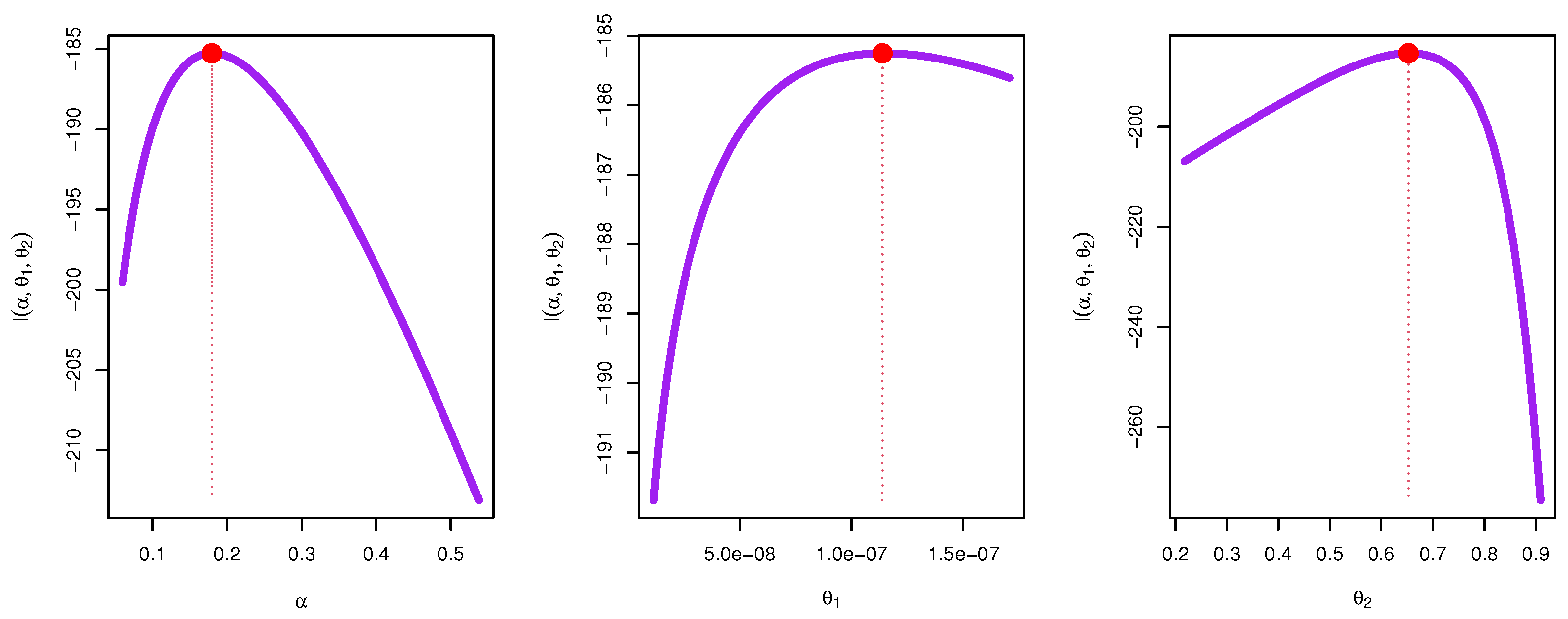
Figure 5 shows the likelihood profiles for model parameters, highlighting peak values, MLEs, and their precision. Steeper curves indicate more reliable estimates, aiding model validation in reliability studies.

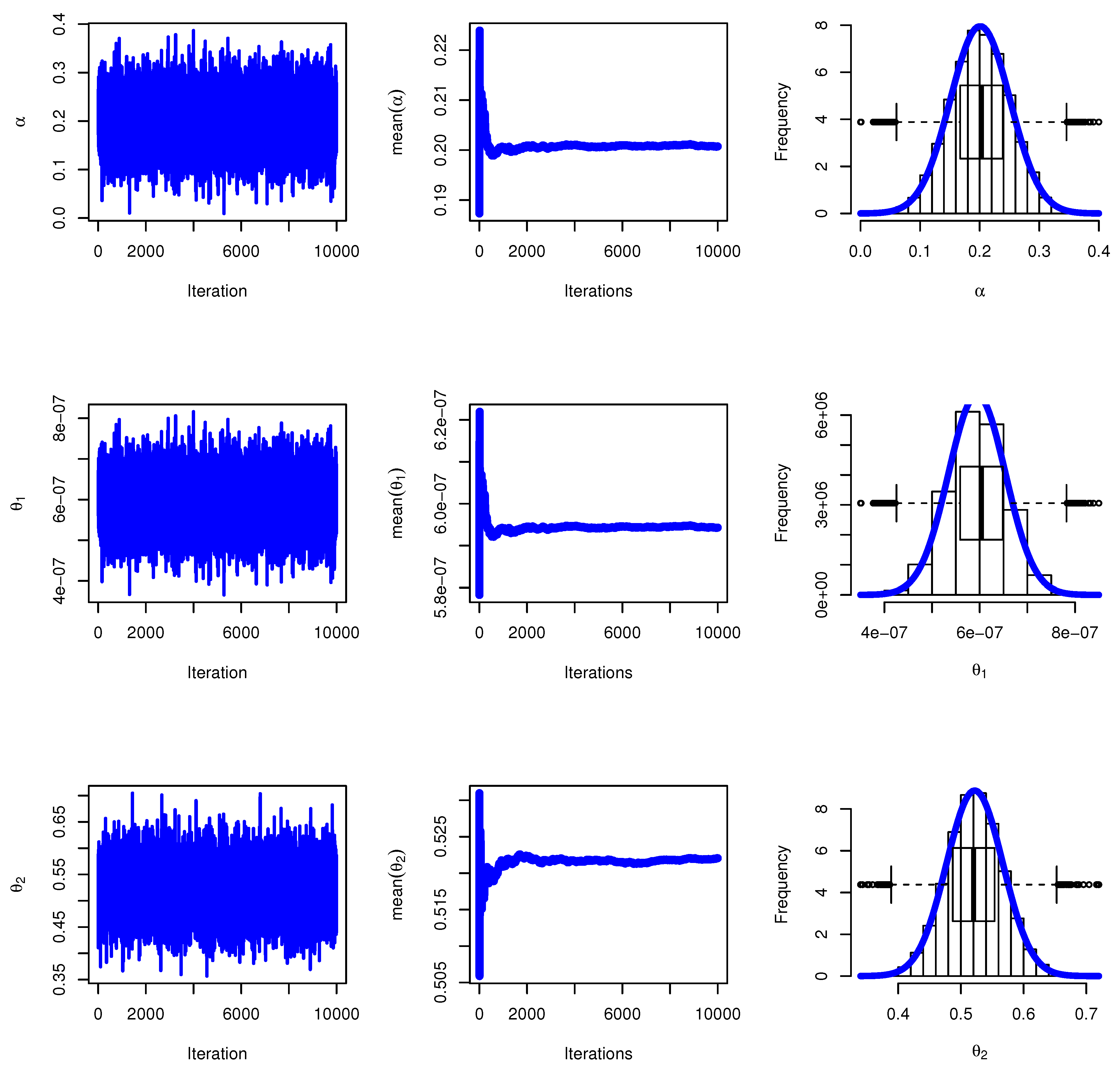
Figure 6 displays MCMC trace plots and posterior distributions for model parameters in a times-to-failure analysis. The trace plots (left) show stable chains with good mixing, indicating convergence, while the posterior densities with normal curves (right) reveal well-identified parameter estimates.

6.2. Data Set II

Ansell and Ansell [50] examined the data set presented in

Table 12. Lifetimes (in cycles) of sodium–sulfur batteries.

Batch 1	164    164    218    230    263    467    538    639    669
	917    1148    1678+    1678+    1678+    1678+
Batch 2	76    82    210    315    385    412    491    504    522
	646+    678    775    884    1131    1446    1824    1827    2248
	2385    3077

Note: Lifetimes with ⁺ are right-censored observations (not failures).

as part of their evaluation of sodium–sulfur battery performance. The data set includes battery lifetimes (measured in cycles) from two different batches. The first batch contained 15 batteries, with four lifetimes being right-censored—these represent the four highest values, all recorded as the same. The second batch consisted of 20 batteries, with only one right-censored lifetime, which is not the highest value in that group. The primary goal of the analysis was to determine whether there was a performance difference between the two batches of batteries. Let these data be considered as an ALT data example, where the first stress factor is temperature. Batteries are typically exposed to elevated temperatures to accelerate their failure mechanisms. The natural use condition is assumed to be 170 °C, while under accelerated stress, the temperature was increased to 200 °C.

Table 13. Likelihood estimates for the parameters and different statistical measures for model under lifetimes of sodium–sulfur batteries data set.

Batch		$\mathit{\alpha }$	${\mathit{\theta }}_1$	${\mathit{\theta }}_2$	AIC	KSD	ADS	CVMS
					BIC	PVKS	PVAD	PVCVM
1	Estimates	1.7342	0.00033	0.1267	234.6540	0.1741	0.0742	0.6077
	StEr	0.2279	0.0000010	0.0630	236.7781	0.7534	0.7334	0.6379
2	Estimates	1.1651	0.000081	0.2028	321.0525	0.1068	0.0367	0.2488
	StEr	0.3515	0.000126	0.1210	324.0397	0.9580	0.9532	0.9709

shows the parameter estimates and goodness-of-fit statistics for the GKME distribution applied to sodium–sulfur battery lifetime data across two batches. Batch 1 has higher shape ($\alpha =1.7342$) and scale (${\theta }_1=0.00033$) parameter estimates compared with Batch 2 ($\alpha =1.1651$, ${\theta }_1=0.000081$), suggesting differences in failure patterns. Both batches exhibit strong model fit, as indicated by high p-values in KSD, ADS, and CVMS tests (all > 0.63), with Batch 1 showing slightly better performance (lower AIC/BIC). The results support the GKME distribution’s suitability for modeling battery lifetimes, though Batch 2’s larger standard errors imply less precision in its estimates.

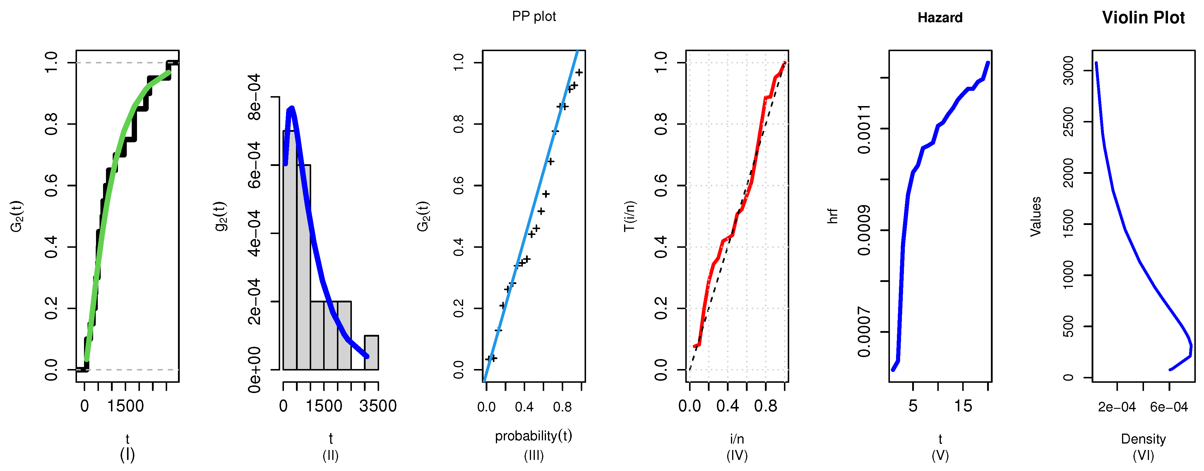
Figure 7 and Figure 8 visually assess the fit of the GKME distribution to the battery lifetime data for two variables. Variable I (Figure 7) and Variable II (Figure 8) likely show how well the theoretical curves align with the empirical data, such as through Q–Q plots or density overlays. The close agreement between the modeled and observed values would support the earlier statistical results (Table 13), confirming the GKME distribution’s effectiveness in capturing the failure patterns of sodium–sulfur batteries. Without the exact images, the figures presumably reinforce the high p-values and low AIC/BIC scores, indicating a robust fit.

Figure 9 displays the likelihood profiles for the GKME distribution parameters fitted to the sodium–sulfur battery lifetime data. The curves likely show how the log-likelihood function varies with changes in parameters like $\alpha$, ${\theta }_1$, and ${\theta }_2$, with peaks indicating MLEs. A well-defined peak would confirm precise parameter estimation, while flat or multi-peaked profiles might suggest identifiability issues of estimates.

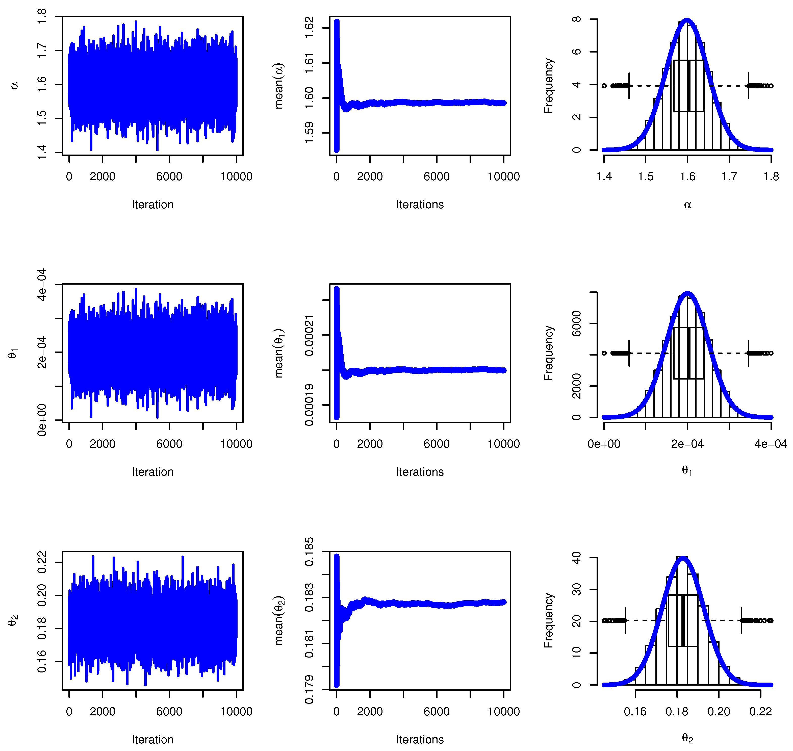
Figure 10 presents the MCMC diagnostic plots for the GKME distribution parameters applied to the sodium–sulfur battery lifetime data. These plots likely include trace plots (showing convergence of chains) and density plots (depicting posterior distributions) for parameters like $\alpha$, ${\theta }_1$, and ${\theta }_2$. Well-mixed, stationary trace plots and smooth, unimodal density curves would indicate robust Bayesian estimation, supporting the reliability of the model.

Table 14. Likelihood estimates and Bayesian estimates for the parameters for model under Lifetimes of sodium sulfur batteries to failure data set.

$({\mathit{m}}_1,{\mathit{m}}_2)$			MLE		Bayes SELF		ELF I	ELF II
$({\mathit{k}}_{\mathbf{1}},{\mathit{k}}_{\mathbf{2}})$	p		Estimates	StEr	Estimates	StEr	Estimates	Estimates
(12, 10) (16, 12)	0.2	$\alpha$	3.0078	0.9145	3.0062	0.0023	3.0062	3.0062
		${\theta }_1$	0.0022	0.0003	0.0023	0.0004	0.0023	0.0023
		${\theta }_2$	0.0190	0.0234	0.0158	0.0018	0.0158	0.0158
	0.9	$\alpha$	1.4513	0.8216	1.4548	0.0021	1.4548	1.4548
		${\theta }_1$	0.0001	0.0002	0.0001	0.00003	0.0001	0.0001
		${\theta }_2$	0.2409	0.2068	0.2337	0.0017	0.2337	0.2337
(12, 10) (16, 12)	0.2	$\alpha$	1.7841	0.7915	1.7830	0.0046	1.7830	1.7830
		${\theta }_1$	0.0003	0.0002	0.0003	0.00007	0.0003	0.0003
		${\theta }_2$	0.1694	0.0210	0.1659	0.0017	0.1659	0.1659
	0.9	$\alpha$	1.5992	0.7025	1.5986	0.0018	1.5992	1.5979
		${\theta }_1$	0.0002	0.0001	0.0002	0.00006	0.0002	0.0002
		${\theta }_2$	0.1828	0.0182	0.1828	0.0032	0.1828	0.1828

compares MLEs and Bayesian estimates (under squared error loss function, SELF, and two other loss functions, ELF I and II) for the GKME distribution parameters ($\alpha$, ${\theta }_1$, ${\theta }_2$) fitted to sodium–sulfur battery failure data. The MLE and Bayesian estimates are notably close, with minor deviations (e.g., $\alpha =3.0078$ vs. $3.0062$ for $p=0.2$), suggesting robustness in parameter estimation. The Bayesian standard errors (StEr) are significantly smaller (e.g., $0.0023$ vs. $0.9145$ for $\alpha$), highlighting the precision of the Bayesian approach. This alignment reinforces the reliability of the GKME model for analyzing battery lifetimes, with both methods yielding consistent results.

Table 15. Likelihood estimates and Bayesian estimates for reliability measures for model under Lifetimes of sodium sulfur batteries to failure data set.

$({\mathit{m}}_1,{\mathit{m}}_2)$		MLE		Bayes SELF		ELF I		ELF II
$({\mathit{k}}_{\mathbf{1}},{\mathit{k}}_{\mathbf{2}})$	p	R	H	R	H	R	H	R	H
(12, 10) (16, 12)	0.2	0.2022	0.2624	0.2034	0.2637	0.2033	0.2637	0.2034	0.2638
	0.9	0.2914	0.3399	0.2721	0.3199	0.2721	0.3199	0.2721	0.3199
(12, 10) (16, 12)	0.2	0.2954	0.3493	0.2782	0.3313	0.2781	0.3313	0.2782	0.3313
	0.9	0.3142	0.3663	0.3153	0.3674	0.3153	0.3674	0.3153	0.3674

presents reliability measures (R) and hazard rates (H) derived from both MLEs and Bayesian methods (SELF, ELF I, ELF II) for the GKME model applied to sodium–sulfur battery failure data. The results, consistent with Table 14 parameter estimates, show close agreement between MLE and Bayesian approaches (e.g., R = 0.203 for $p=0.2$), with minor variations (e.g., R = 0.2914 vs. 0.2721 for $p=0.9$). This alignment confirms the model’s robustness in predicting reliability, while the Bayesian estimates exhibit slightly lower hazard rates (H), suggesting a more conservative assessment of failure risk. The findings reinforce the GKME distribution’s utility for reliability analysis in battery lifetime studies.

7. Conclusions

This study examines progressive-stress ALT for the lifespan GKME distribution based on a generalized progressive hybrid censoring framework, illustrating the recommended methodologies with a real example. MLE and Bayesian estimates of the parameters were obtained for several sample sizes and two binomial parameter configurations for random elimination, with their efficacy evaluated using mean squared errors. The results of the simulation exercise demonstrate that Bayesian point estimates and the highest posterior density credible intervals surpass traditional point estimates derived from bootstrap methods. This pattern was likewise evident in two empirical data studies. The analysis, utilizing statistical metrics including AIC, BIC, KSD, and p-values, indicates that the GKME distribution derived from progressive-stress ALT surpasses the competing models.