Article

Generalized Logistic Maps in the Complex Plane: Structure, Symmetry, and Escape-Time Dynamics

by
Krzysztof Gdawiec
1,* and
Muhammad Tanveer
2
1
Institute of Computer Science, University of Silesia in Katowice, Bedzinska 39, 41-200 Sosnowiec, Poland
2
Department of Mathematics and Statistics, Sub-Campus Depalpur, University of Agriculture Faisalabad, Faisalabad 38000, Pakistan
*
Author to whom correspondence should be addressed.
Axioms 2025, 14(6), 404; https://doi.org/10.3390/axioms14060404
Submission received: 11 April 2025 / Revised: 17 May 2025 / Accepted: 21 May 2025 / Published: 26 May 2025
(This article belongs to the Special Issue Trends in Dynamical Systems and Applied Mathematics)

Abstract

:
In this paper, we introduce a generalised formulation of the logistic map extended to the complex plane and correspondingly redefine the classical Mandelbrot and Julia sets within this broader framework. Central to our approach is the development of an escape criterion based on the Picard orbit, which underpins the escape-time algorithms employed for graphical approximations of these sets. We analyse the structural and dynamical properties of the resulting Mandelbrot and Julia sets, emphasising their inherent symmetries through detailed visualisations. Furthermore, we examine how variations in a key parameter of the generalised map affect two critical numerical metrics: the average escape time and the non-escaping area index. Our computational study reveals that, particularly for Julia sets, these dependencies are characterised by intricate, highly non-linear behaviour—highlighting the profound complexity and sensitivity of the system under this generalised mapping.
MSC:
47H10; 47J25; 37F45

1. Introduction

Mandelbrot and Julia sets are probably the most recognisable fractal sets. Mandelbrot introduced them in [1]. Mandelbrot based his findings on the results of Pierre Fatou and Gaston Julia, who studied the Julia sets at the beginning of the 20th century. However, they were not able to draw those sets. During his work at IBM, Mandelbrot was the first to draw them using a computer. He was fascinated by these sets and started to study their connectedness and marked values of the parameter for which the Julia sets were connected. In this way, the Mandelbrot arose. Since then, much research has been conducted on Mandelbrot and Julia sets. Moreover, these sets found many applications. For example, in the design of textile [2] and garment [3] patterns, in fashion [4] design, and in designing microstrip patch antennas [5], image compression and encryption [6], etc.
The original Mandelbrot and Julia sets were obtained for the polynomial z 2 + c , where c C is a parameter, and the Picard feedback iteration process [7]. Later on, many researchers investigated various modifications of the function and the feedback iteration process. For example, iterations such as the Mann [8,9,10], Picard–Mann [11,12], viscosity [13], S-iteration [14], Jungck–Ishikawa with s-convexity [15], Jungck–Mann with s-convexity [16] were used. The quadratic function was replaced, for example, by a higher-order polynomial function [17], rational [18], or Möbius [19] functions. One of the most interesting functions that was considered is the logistic map.
In [20], Rani and Agarwal studied fractal generation with the use of Mann iteration and the classical logistic map:
g ( z ) = r z ( 1 z ) ,
where r C is a parameter. Later, in [21], they studied the effect of using noise in the Julia sets obtained using (1). The classical logistic map was also studied by Prasad and Katiyar. In their study presented in [22], they studied the use of the Ishikawa iteration in the generation of fractal patterns. Except for the classical version of the logistic map, some generalisations and modifications were studied in the literature. For example, in [23], Ahmed et al. studied the following version of the logistic map:
h ( z ) = α z ( 1 z ) β ,
where α C and β N , in the generation of Mandelbrot sets. Next, in [24], Xiangyuan and Qingyong introduced a modified complex compound logistic map of the following form:
p ( z ) = η 4 z ( 1 z ) z ( 1 z ) 3 8 + c ,
where η , c C , and studied its Mandelbrot and Julia sets.
In this paper, we propose a new generalisation of the logistic map and define Mandelbrot and Julia sets for it. Then, we study the properties of the proposed fractal sets, that is, the escape conditions and the symmetries. We also show some graphical and numerical examples for the considered Mandelbrot and Julia sets.
The rest of the paper is organised as follows. In Section 2, we introduce the generalised logistic map and define Mandelbrot and Julia sets for this type of mapping. Moreover, we prove the escape criterion and study the symmetries of the proposed sets. Next, in Section 3, we introduce escape-time algorithms for generating Mandelbrot and Julia sets of the generalised logistic map and present some graphical examples of those sets. Section 4 is devoted to numerical examples in which we study the dependency between the s parameter that defines the proposed logistic map and two numerical measures used in the literature. Finally, in Section 5, we conclude our findings and give directions for future study.

2. Generalised Logistic Map and Its Mandelbrot and Julia Sets

Throughout the rest of the paper, we understand that the set of natural numbers starts from zero, i.e., N = { 0 , 1 , 2 , } .
In this section, we introduce and study Mandelbrot and Julia sets for the generalised logistic map f r : C C of the form
f r ( z ) = r z ( s z m ) ,
where m N , m 2 , s C , and r C { 0 } . We start our considerations with the definitions of these two sets.
Definition 1.
The filled Julia set F of the generalised logistic map (4) is the set of points z 0 C whose Picard orbit, i.e.,
z n + 1 = f r ( z n ) = f r n + 1 ( z 0 )
do not tend to infinity, i.e.,
F =   { z 0 C : { | z n | } n = 0 r e m a i n s b o u n d e d } .
The boundary of F is called the Julia set J , that is, J = F .
Definition 2.
The Mandelbrot set M of (4) is defined in the following way
M = { r C : | f r n ( η ) | a s n } ,
where η is a critical point of the generalised logistic map, i.e., η = s 1 + m 1 m .

2.1. Escape Criterion

In Definitions 1 and 2, we check the escaping of the orbit for a given starting point. Thus, let us study the conditions under which the orbit escapes to infinity.
Theorem 1.
Let us consider the generalised logistic map given in (4). Let z 0 C be such that
| z 0 |   > 1 + | r | ( 1 + | s | ) | r | 1 m
and that { z n } n N is the Picard orbit of z 0 , i.e.,
z n + 1 = f r ( z n ) = r z n s z n m
for n N . Then, lim n | z n | = .
Proof. 
For n = 0 , we have
| z 1 | = | r z 0 ( s z 0 m ) | = | r | | z 0 | | s z 0 m | | r | | z 0 | ( | z 0 m |     | s | ) > | r | | z 0 | ( | z 0 m |     ( 1 + | s | ) ) 1 + | s | > | s | .
Since | z 0 | > 1 + | r | ( 1 + | s | ) | r | 1 m , then
| r | | z 0 m |     ( 1 + | s | ) > 1 .
Therefore, there exists ζ > 0 such that
| r | | z 0 m |     ( 1 + | s | ) > 1 + ζ .
Thus,
| z 1 | > ( 1 + ζ ) | z 0 | .
In particular, | z 1 |   >   | z 0 | , so we can apply the same argument repeatedly to obtain
| z n |   > ( 1 + ζ ) n | z 0 | .
Hence, lim n | z n | = . □
From Theorem 1, we see that when the starting point z 0 of the Picard orbit is outside a ball centred at the origin with radius R = 1 + | r | ( 1 + | s | ) | r | 1 m (see (8)), then the point escapes to infinity. This means that the points outside of this ball do not belong to the filled Julia set. Thus, the filled Julia set is contained in the ball with radius R and centred at the origin.
Using similar reasoning as in the proof of Theorem 1, we can prove the following theorem.
Theorem 2.
Let us consider the generalised logistic map given in (4). Suppose that for the Picard orbit of z 0 C , we have
| z j |   > 1 + | r | ( 1 + | s | ) | r | 1 m ,
for some j 0 . Then, lim n | z n | = .
Theorem 2 gives us the so-called escape criterion. From this theorem, we see that if for some j 0 , the corresponding element of the orbit exceeds 1 + | r | ( 1 + | s | ) | r | 1 m , then the orbit escapes to infinity. Using this fact, we can construct an escape-time algorithm for generating the Mandelbrot and Julia sets for the considered generalised logistic map. The algorithms will be introduced in Section 3.

2.2. Symmetries of the Julia Sets

One of the interesting properties studied in the classical Mandelbrot and Julia sets is the symmetries of those sets. Now, we concentrate on this matter in the context of the Julia sets for the considered generalised logistic map.
Theorem 3.
Let us consider the generalised logistic map given in (4). Let α = 2 π m and k { 0 , 1 , , m 1 } . Then,
| f r n ( z e i k α ) | = | f r n ( z ) |
for all n N and z C .
Proof. 
We start by proving that for all n N and z C
f r n ( z e i k α ) = f r n ( z ) e i k α .
We prove (12) by induction. For n = 1 , we have
f r ( z e i k α ) = r z e i k α ( s [ z e i k α ] m ) = e i k α r z ( s z m e i k m α ) .
Because α = 2 π m ,
e i k m α = e i 2 π k = 1 .
Thus,
f r ( z e i k α ) = e i k α r z ( s z m ) = e i k α f r ( z ) .
Assume that the statement is true for some n 1 , i.e.,
f r n ( z e i k α ) = f r n ( z ) e i k α .
For n + 1 , we have
f r n + 1 ( z e i k α ) = f r ( f r n ( z e i k α ) ) .
From the inductive hypothesis (14), we obtain
f r ( f r n ( z e i k α ) ) = f r ( f r n ( z ) e i k α ) .
Because (13) is true for all z C , we obtain
f r n + 1 ( z e i k α ) = f r ( f r n ( z ) e i k α ) = e i k α f r ( f r n ( z ) ) = e i k α f r n + 1 ( z ) .
Therefore, (12) follows by induction for all n N .
Now, by using (12), we obtain
| f r n ( z e i k α ) | = | f r n ( z ) e i k α | = | f r n ( z ) | .
This completes the proof. □
Theorem 3 shows that if we take any point z 0 C and it is rotated by k α version, i.e., z 0 = z 0 e i k α , then the corresponding sequences { | z n | } n = 0 and { | z n | } n = 0 will be the same. This means that the Julia set of the generalised logistic map has m-fold rotational symmetry.
Theorem 4.
Let us consider the generalised logistic map given in (4). Let m be even, then
| f r n ( z ) | = | f r n ( z ) |
for all n N and z C .
Proof. 
We start by proving that if m is even, then for all n N and z C
f r n ( z ) = f r n ( z ) .
We prove (16) by induction. For n = 1 , we have
f r ( z ) = r ( z ) ( s ( z ) m ) = r z ( s z m ) = f r ( z ) .
Assume that the statement is true for some n 1 , i.e.,
f r n ( z ) = f r n ( z ) .
For n + 1 , we have
f r n + 1 ( z ) = f r ( f r n ( z ) ) .
From the inductive hypothesis (17), we obtain
f r n + 1 ( z ) = f r ( f r n ( z ) ) = r ( f r n ( z ) ) ( s ( f r n ( z ) ) m ) = r f r n ( z ) ( s ( f r n ( z ) ) m ) = f r ( f r n ( z ) ) = f r n + 1 ( z ) .
Therefore, (16) follows by induction for all n N .
Now,
| f r n ( z ) | = | f r n ( z ) | = | f r n ( z ) | .
This completes the proof. □
From Theorem 4, we see that if we take any z 0 C and z 0 = z 0 , then the corresponding sequences { | z n | } n = 0 and { | z n | } n = 0 will be the same. This means that for even values of m, the Julia set of the generalised logistic map is symmetric with respect to the origin.

2.3. Symmetries of the Mandelbrot Set

In this subsection, we study the symmetries of the Mandelbrot sets obtained for the generalised logistic map.
Theorem 5.
Let f r ( z ) = r z ( s z m ) , where m N , m 2 , s C , and r C { 0 } . Let α = 2 π m and k { 0 , 1 , , m 1 } . Then,
| f r e i α n ( z ) | = | f r n ( z ) | ,
for all n N , z C , and r C { 0 } .
Proof. 
We start by proving that for all n N and z C
f r e i α n ( z ) = e i n α f r n ( z ) .
We prove (20) by induction. For n = 1 , we have
f r e i α ( z ) = r e i α z ( s z m ) = e i α f r ( z ) .
Assume that the statement is true for some n 1 , i.e.,
f r e i α n ( z ) = e i n α f r n ( z ) .
For n + 1 , we have
f r e i α n + 1 ( z ) = f r e i α ( f r e i α n ( z ) ) .
From the inductive hypothesis (21), we obtain
f r e i α ( f r e i α n ( z ) ) = f r e i α ( e i n α f r n ( z ) ) = r e i α e i n α f r n ( z ) ( s [ e i n α f r n ( z ) ] m ) = e i ( n + 1 ) α r f r n ( z ) ( s e i m n α [ f r n ( z ) ] m ) .
Because α = 2 π m ,
e i m n α = e i 2 π n = 1 .
Thus,
f r e i α n + 1 ( z ) = e i ( n + 1 ) α r f r n ( z ) ( s [ f r n ( z ) ] m ) = e i ( n + 1 ) α f r ( f r n ( z ) ) = e i ( n + 1 ) α f r n + 1 ( z ) .
Therefore, (20) follows by induction for all n N .
Now, by using (20), we obtain
| f r e i α n ( z ) | = | e i n α f r n ( z ) | = | f r n ( z ) | .
This completes the proof. □
Theorem 5 shows that if we take any r C { 0 } and it is rotated by k α version, i.e., r = r e i k α , then the corresponding sequences { | f r n ( η ) | } n = 0 and { | f r n ( η ) | } n = 0 will be the same. This means that the Mandelbrot set of the generalised logistic map has m-fold rotational symmetry.
Theorem 6.
Let f r ( z ) = r z ( s z m ) , where m N , m 2 , s C , and r C { 0 } . Let m be even, then
| f r n ( z ) | = | f r n ( z ) | ,
for all n N , z C , and r C { 0 } .
Proof. 
By induction, we can show that if m is even, then for all n N , z C , and r C { 0 }
f r n ( z ) = f r n ( z ) , if n is odd , f r n ( z ) , if n is even .
Now,
| f r n ( z ) | = | f r n ( z ) | , if n is odd , | f r n ( z ) | , if n is even .
Thus, | f r n ( z ) | = | f r n ( z ) | . □
From Theorem 6, we see that if we take any r C { 0 } and r = r , then the corresponding sequences { | f r n ( η ) | } n = 0 and { | f r n ( η ) | } n = 0 will be the same. This means that for even values of m, the Mandelbrot set of the generalised logistic map is symmetric with respect to the origin.

3. Graphical Examples

In Theorem 2, we proved the so-called escape criterion. In this section, we use it to introduce algorithms for the generation of approximation of the Mandelbrot and Julia sets for the generalised logistic map. Moreover, we present some graphical examples obtained with those algorithms.

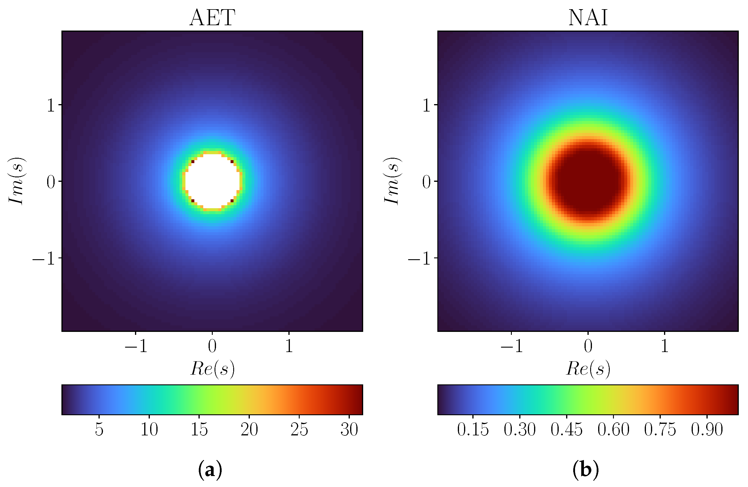
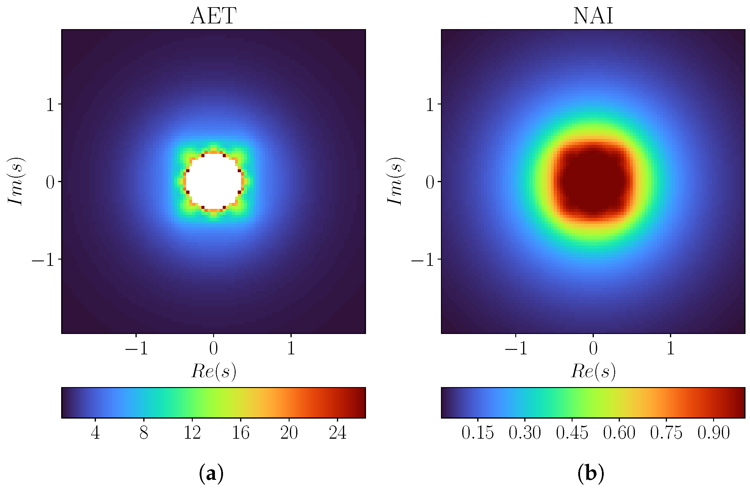
3.1. Mandelbrot Sets

In Algorithm 1, we present the pseudocode of the escape-time algorithm for the generation of the approximation of the Mandelbrot set for the generalised logistic map. In this algorithm, for each r A , which is treated as a parameter in the f r function, we iterate the f r starting from the critical point s 1 + m 1 m . In each iteration, we check whether the point has escaped, i.e., the modulus of the current iterate has exceeded R. Moreover, to avoid an infinite loop in the case of non-escaping points, we also check whether the current iteration number has not exceeded the maximal number of iterations K. In the final step, we colour the starting point according to the number of performed iterations using the chosen colour map.
Algorithm 1: Approximation of Mandelbrot set
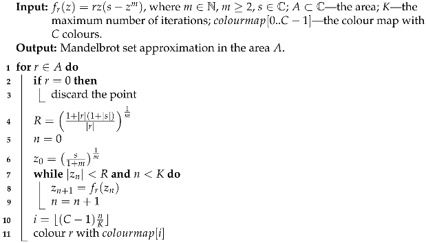
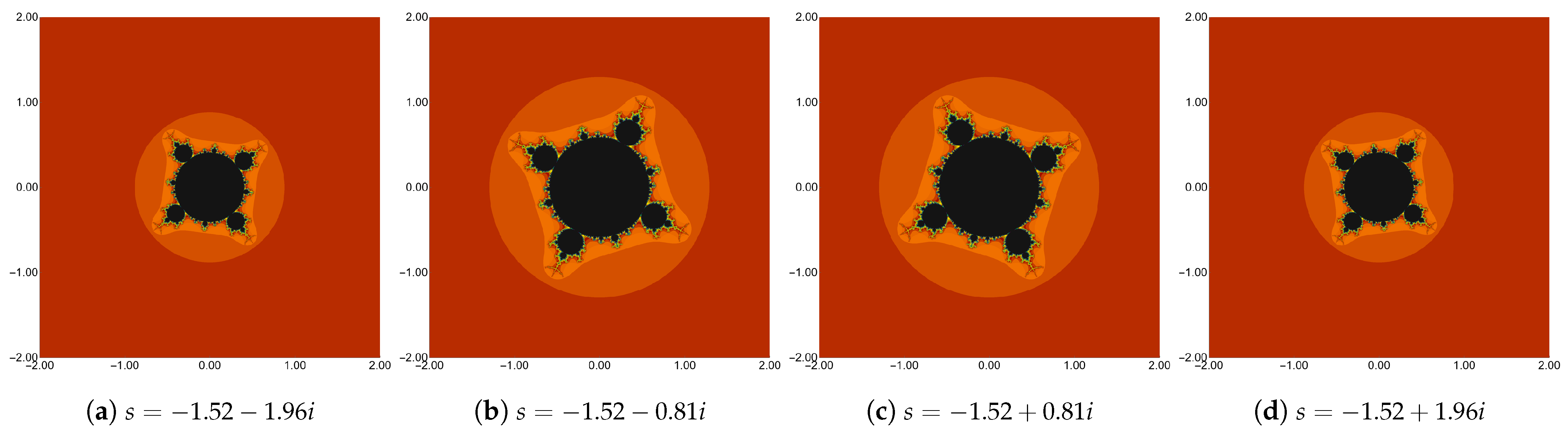
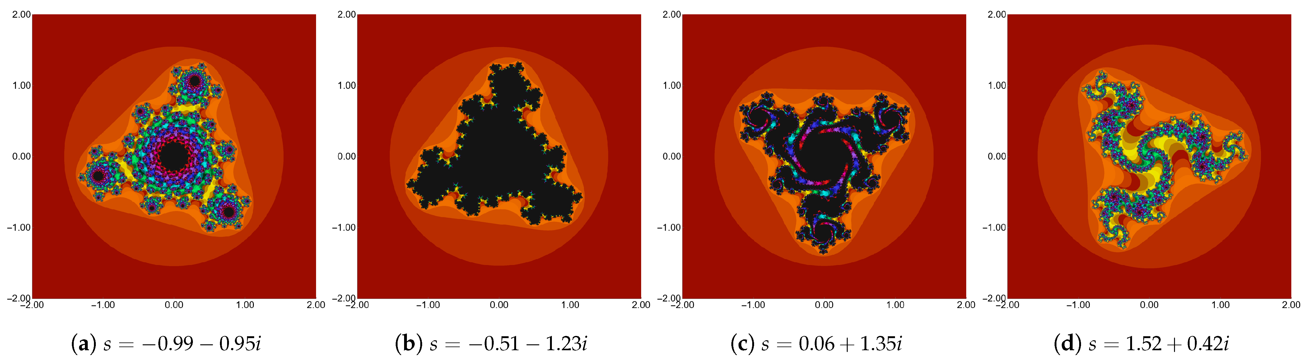
Axioms 14 00404 i001
In the examples, we show approximations of Mandelbrot sets for two values of m (3, 4) and varying values of s in the generalised logistic map. To generate images of those sets, we used Algorithm 1 implemented in Mathematica and the following common parameters: A = [ 2 , 2 ] 2 , K = 50 , and the colour map presented in Figure 1.
Images of approximation of Mandelbrot sets obtained for m = 3 are presented in Figure 2. The values of s were selected so that the real part is fixed at 0.5 and the imaginary part varies. The images show that the approximation of the Mandelbrot set for each value of s has the same shape. In each image, we can observe one main bulb and three bulbs of the same radius connected to this main bulb. The only difference between the images is in the scale and rotation of the set. Moreover, we can observe that the set approximation has 3-fold rotational symmetry, which is in accordance with the theoretical results proved in Section 2. In the example, we fixed the real part of s. For other values of the real part, we can observe a similar behaviour. Also, when we fix the imaginary part and vary the real part, the behaviour is the same, i.e., the set approximation has the same shape, and only differs in scale and rotation angle.
In Figure 3, we see the images of the approximations of the Mandelbrot set obtained for m = 4 and varying values of s. As in the previous example, we fixed the real part of s, this time at 1.52 , and varied the imaginary part. From the images, we can observe a very similar behaviour to the one we saw for m = 3 . Namely, the shape of the set approximation for each value of s is the same, but this time, we see one main bulb and four bulbs of the same radius connected with the main bulb. The difference is in the scale and the rotation angle. Moreover, we can see that each of the sets’ approximations has 4-fold rotational symmetry and that the sets’ approximations are symmetric with respect to the origin, which corresponds to the theoretical results from Section 2. As for m = 3 , similar behaviour is observable when we change the value of the real part of s or fix the imaginary part of s and vary its real part.

3.2. Julia Sets

The pseudocode for the generation of the approximation of filled Julia sets for the generalised logistic map is presented in Algorithm 2. The algorithm is very similar to the one for the Mandelbrot set approximation. The difference is in the starting point for the feedback process. In the Mandelbrot set case, the point from A was the parameter for the function f r , and the starting point was set as the critical point of f r . For the filled Julia set approximation, we see that the point from A is the starting point. This difference is a consequence of the definitions of these two sets.
Algorithm 2: Approximation of filled Julia set
Axioms 14 00404 i002
Like in the examples for the Mandelbrot set, we present graphical examples for m = 3 , 4 in the generalised logistic map defining the considered Julia sets. To generate the corresponding images, we used Algorithm 2 implemented in Mathematica. The parameters used in the algorithm were the following:
  • m = 3 , r = 0.75 i , A = [ 2 , 2 ] 2 , K = 50 , the colour map from Figure 1,
  • m = 4 , r = 0.5 + 0.5 i , A = [ 1.5 , 1.5 ] 2 , K = 50 , the colour map from Figure 1.
The obtained cubic ( m = 3 ) Julia sets’ approximations for various values of s are presented in Figure 4. For these sets, we see that various shapes can be obtained for different values of s. This behaviour differs from the one we saw in the Mandelbrot set case. The values of s were selected in such a way that we see a variety of shapes that can be obtained. In the images, we see that the approximations of filled Julia sets (points coloured using black colour) occupy different areas, and some of them reveal spiral structures. All the sets’ approximations have the 3-fold rotational symmetry, which corresponds to the results that we proved in Section 2.
In the last graphical example, we present an approximation of filled Julia sets obtained with the generalised logistic map in which we set m = 4 and r = 0.5 + 0.5 i . The obtained images for various values of s are presented in Figure 5. As for the cubic case, the sets’ approximations in Figure 5 have various shapes and contain some spiral structures. The filled Julia sets’ approximations again have various sizes. In Figure 5c, we see the largest set approximation (the black area), whereas the smallest set approximations are visible in Figure 5a,d. The dependency between s and the size will be the subject of the study in the next section. The sets’ approximations in Figure 5 are all symmetric, where we can observe the 4-fold rotational symmetry and the symmetry with respect to the origin. Again, this aligns with the theorems proved in Section 2.

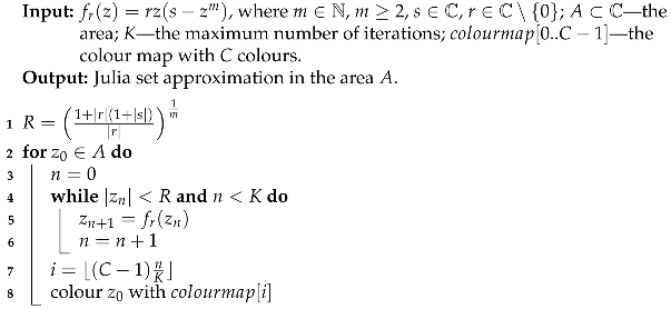
4. Numerical Examples

In Section 3, we saw that for the Julia sets, we can obtain sets of various shapes and sizes. In this section, we study the dependency between the values of s and the corresponding Mandelbrot and Julia sets. The dependencies between parameters of some iteration processes and the Mandelbrot and Julia sets can be very interesting. For example, in [25], Kumari et al. showed that such dependency for the viscosity iteration can reveal a fractal nature. Various numerical measures are used in the literature to study such dependencies.
In this section, we use two recently introduced measures: the average escape time (AET) and the non-escaping area index (NAI). They were introduced in [13]. These two measures are calculated using two different sets of points. AET is computed from the escaping point as the average number of iterations, which shows how fast, on average, the points escape to infinity. NAI is computed using the non-escaping points as the ratio of the number of non-escaping points to the number of points in the considered area. Thus, NAI is the percentage of the considered area covered by the Mandelbrot or filled Julia set, so it gives us information on the relative size of the set in the area.
To show the dependency between the parameter s C and the two numerical measures, we need to generate Mandelbrot and Julia sets for various values of s, calculate the measures, and then plot the data. For all the presented plots in this section, we used the same parameters as for the graphical examples presented in Section 3. For the varying parameter s, we generated equally spaced 100 values in ( 2 , 2 ) (Mandelbrot set case) and [ 2 , 2 ] (for the Julia set case) for the real and imaginary parts, which gives 10,000 images generated for a single plot. The resolution of the generated images was set to 800 × 800 pixels. The escape-time algorithms for generating the sets were implemented in Mathematica, and for creating the plots with the numerical measures, the Python’s matplotlib library was used.

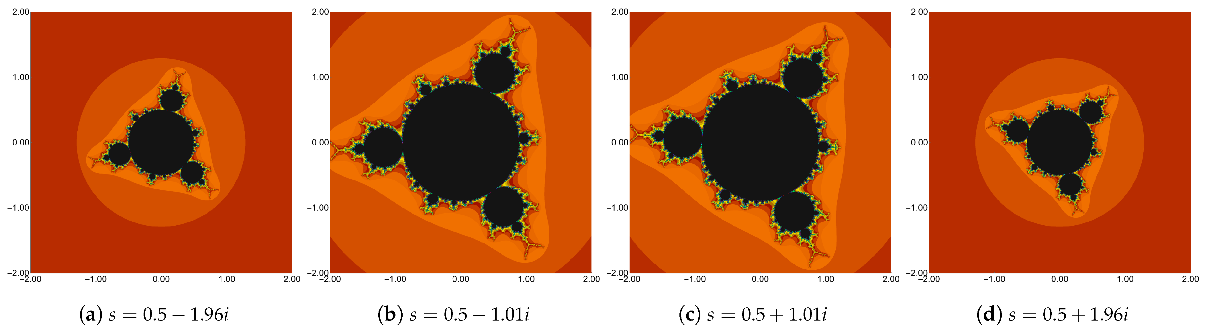
4.1. Mandelbrot Sets

The obtained AET and NAI plots for the Mandelbrot set with m = 3 are presented in Figure 6. The white area in the centre of the AET plot shows the values of s for which we were not able to calculate this measure, because all points in the considered area were non-escaping ones. From the plot, we see that the highest values of AET are obtained near the boundary of the white area. The maximal value of 31.320 is reached for s = 0.257 0.257 i , s = 0.257 + 0.257 i , s = 0.257 0.257 i , and s = 0.257 + 0.257 i . We see these points as dark red points placed symmetrically. When we move radially away from the origin, we observe that the AET values decrease, obtaining the lowest values at the boundaries of the considered area. The minimal value of 1.303 is reached, for example, for s = 1.960 1.960 i . When we look at the NAI plot, we notice very similar behaviours in this measure. The highest values are visible in the neighbourhood of the origin. The value of NAI in this area is equal to 1.0 , which means that the Mandelbrot set covered the whole area A. Then, if we move radially from the centre, the value of NAI gradually decreases and obtains the lowest value equal to 0.037 at s = 1.960 1.960 i . This shows that the size of the Mandelbrot set for m = 3 depends on the modulus of s, i.e., the higher the modulus, the smaller the set is. We can observe this in Figure 2, where for (a) and (d) | s | 2.022 the sets are small, and for (b) and (c) | s | 1.126 the sets are large.
The AET and NAI plots for the second Mandelbrot set ( m = 4 ) are presented in Figure 7. In the AET plot, we see a white area around the origin, as in the case of the cubic Mandelbrot set, and that the area is less circular. The highest values of AET are visible as dark red points in the plot. They correspond to the value equal to 26.296 . These points are again placed in a symmetric way in the parameters’ plane, i.e., they belong to the set { 0.337 0.139 i , 0.337 + 0.139 i , 0.139 0.337 i , 0.139 + 0.337 i ,   0.139 0.337 i ,   0.139 + 0.337 i , 0.337 0.139 i , 0.337 + 0.139 i } . The values around the boundary of the white region form an irregular, symmetric shape. When we move away from this boundary, the value of AET decreases radially. The minimal value equal to 1.222 is reached near the boundaries of A, for example, at s = 1.96 1.96 i . In the NAI plot, we see that, again, the highest value equal to 1.0 is in the central part of the plot, which corresponds to the white region in the AET plot. The values of NAI depend on the modulus of s, i.e., the higher the modulus, the lower the NAI value, which means a smaller Mandelbrot set. The minimal value equal to 0.034 is reached, for example, for s = 1.96 1.96 i . The graphical examples presented in Figure 3 show this observation, because the modulus of s for the smaller sets in (a) and (d) is approximately equal to 2.480 , whereas for the bigger sets in (b) and (c) it is approximately equal to 1.722 .

4.2. Julia Sets

The obtained AET and NAI plots for the cubic Julia sets from Section 3 are presented in Figure 8. In the AET plot, we do not see any white points, so for all values of s, there were some escaping points. The lowest values of the AET measure are visible in the neighbourhood of the origin, where the minimal value equal to 0.186 was reached for s = 0.02 0.02 i . When we look at the points with high values of AET, we notice that they form a complex shape that resembles the boundaries of the cubic Mandelbrot set presented in Figure 2. The maximal value equal to 3.990 is reached for s = 0.182 1.350 i . If we move away from the points with the highest values of AET, then again, the values of AET are relatively low. For the NAI plot, we also see a shape that reminds us of the shape of the cubic Mandelbrot set in Figure 2. The lowest values of NAI equal to 0.0 are obtained for the values of s outside of the set, whereas the highest are inside it. The maximal value equal to 0.237 is reached for s = 0.02 0.02 i . From the NAI plot, we see that determining the size of the Julia set is challenging because of the complex shape of the dependency between the values of s and NAI.
In Figure 9, we see the AET and NAI plots for the last numerical example; that is, for the Julia sets generated for m = 4 and r = 0.5 + 0.5 i . In the plots, we can observe a similar behaviour to the one that we observed for the cubic Julia set. Namely, for the AET plot, the highest values of this numerical measure form a very complex shape that resembles the Mandelbrot set from Figure 3. The maximal value of AET is equal to 6.725 , and it is reached for s = 0.909 1.110 i . The lowest values of AET are visible in the central part of the plot (the minimal value 0.271 is at s = 0.02 0.02 i ), which corresponds to the interior of the complex shape. Values a little higher are obtained for s that lie outside the complex shape. For the NAI plot, we also see a shape that reminds us of the Mandelbrot set from Figure 3. Outside of this complex set, the NAI is equal to 0.0 . For the values of s inside the shape, we observe high values of NAI, where the maximal value of 0.414 is reached for s = 0.02 0.02 i . Thus, as in the case of the cubic Julia set, the dependency between s and the relative set size is complex and non-linear.

5. Conclusions and Future Work

In this paper, we introduced Mandelbrot and Julia sets for a generalised version of the logistic map. For these sets, we proved the escape criterion which is the base for a standard visualisation algorithm, the so-called escape-time algorithm. We also studied the symmetries of the proposed sets. Moreover, we presented some graphical and numerical examples. The graphical examples showed that very interesting shapes of the sets can be obtained. On the other hand, the numerical examples showed that the dependency between the value of the s parameter and two numerical measures can be different for Mandelbrot and Julia sets. For the Mandelbrot set, we observed that this dependency is simple and relies on the modulus of s. Whereas, for the Julia sets, we observed complex shapes that remind us of the Mandelbrot sets of the corresponding degree m of the logistic map.
Because the dependencies between s and the numerical measures are very complex for the Julia sets and the space for s is broad, manually finding interesting set shapes is tedious. Therefore, developing an automatic method for the search process would be interesting. For the classical function z m + c and its variations, we can find numerous papers on the use of various iteration processes from the fixed-point theory. See, for example, [11,12,14,26]. Thus, another direction for future study can be the use of various iteration processes instead of the Picard iteration used in this paper for the generalised logistic map.

Author Contributions

K.G.: Conceptualization, Formal Analysis, Investigation, Software, Visualization, Writing—original draft, Writing—review & editing; M.T.: Conceptualization, Investigation, Validation, Writing—review & editing. All authors have read and agreed to the published version of the manuscript.

Funding

This research received no external funding.

Data Availability Statement

The data that support the findings of this study are available from the corresponding author, upon reasonable request.

Conflicts of Interest

The authors declare that they have no conflicts of interest.

References

  1. Mandelbrot, B. The Fractal Geometry of Nature; W.H. Freeman and Company: San Francisco, CA, USA, 1982. [Google Scholar]
  2. Feijs, L.; Toeters, M. Exploring a Taxicab-based Mandelbrot-like Set. In Proceedings of the Bridges 2019: Mathematics, Art, Music, Architecture, Education, Culture, Linz, Austria, 16–20 July 2019; Goldstine, S., McKenna, D., Fenyvesi, K., Eds.; Tessellations Publishing: Phoenix, AZ, USA, 2019; pp. 107–114. [Google Scholar]
  3. Wang, W.; Zhang, G.; Yang, L.; Wang, W. Research on garment pattern design based on fractal graphics. EURASIP J. Image Video Process. 2019, 2019, 29. [Google Scholar] [CrossRef]
  4. Toeters, M.; Feijs, L.; van Loenhout, D.; Tieleman, C.; Virtala, N.; Jaakson, G.K. Algorithmic Fashion Aesthetics: Mandelbrot. In Proceedings of the 23rd International Symposium on Wearable Computers (ISWC ’19), New York, NY, USA, 9–13 September 2019; pp. 322–328. [Google Scholar] [CrossRef]
  5. Venneri, F.; Costanzo, S.; Borgia, A. Fractal Metasurfaces and Antennas: An Overview for Advanced Applications in Wireless Communications. Appl. Sci. 2024, 14, 2843. [Google Scholar] [CrossRef]
  6. Yang, J.; Feng, X.; Chen, Y.; Yan, P.; Zhang, H. A secure fractal compression scheme based on irregular Latin square, Julia and 2D-FCICM. Digit. Signal Process. 2024, 155, 104725. [Google Scholar] [CrossRef]
  7. Devaney, R. A First Course in Chaotic Dynamical Systems: Theory and Experiment, 2nd ed.; CRC Press: Boca Raton, FL, USA, 2020. [Google Scholar]
  8. Rani, M.; Kumar, M. Circular saw Mandelbrot set. In Proceedings of the the 14th WSEAS International Conference on Applied Mathematics, Puerto De La Cruz, Tenerife Canary Islands, Spain, 14–16 December 2009; pp. 131–136. [Google Scholar]
  9. Rani, M.; Kumar, V. Superior Mandelbrot set. J. Korea Soc. Math. Educ. Ser. D Res. Math. Educ. 2004, 8, 279–291. [Google Scholar]
  10. Rani, M.; Kumar, V. Superior Julia sets. J. Korea Soc. Math. Educ. Ser. D Res. Math. Educ. 2004, 8, 261–277. [Google Scholar]
  11. Adhikari, N.; Sintunavarat, W. The Julia and Mandelbrot Sets for the Function zpqz2 + rz + sin cw Exhibit Mann and Picard–Mann Orbits Along with s-convexity. Chaos Solitons Fractals 2024, 181, 114600. [Google Scholar] [CrossRef]
  12. Tanveer, M.; Nazeer, W.; Gdawiec, K. On the Mandelbrot Set of zp + log ct via the Mann and Picard–Mann Iterations. Math. Comput. Simul. 2023, 209, 184–204. [Google Scholar] [CrossRef]
  13. Kumari, S.; Gdawiec, K.; Nandal, A.; Kumar, N.; Chugh, R. On the Viscosity Approximation Type Iterative Method and Its Non-linear Behaviour in the Generation of Mandelbrot and Julia Sets. Numer. Algorithms 2024, 96, 211–236. [Google Scholar] [CrossRef]
  14. Srivastava, R.; Tassaddiq, A.; Kasmani, R. Escape Criteria Using Hybrid Picard S-Iteration Leading to a Comparative Analysis of Fractal Mandelbrot Sets Generated with S-Iteration. Fractal Fract. 2024, 8, 116. [Google Scholar] [CrossRef]
  15. Antal, S.; Tomar, A.; Prajapati, D.; Sajid, M. Variants of Julia and Mandelbrot sets as fractals via Jungck–Ishikawa fixed point iteration system with s-convexity. AIMS Math. 2022, 7, 10939–10957. [Google Scholar] [CrossRef]
  16. Tomar, A.; Prajapati, D.; Antal, S.; Rawat, S. Variants of Mandelbrot and Julia fractals for higher-order complex polynomials. Math. Methods Appl. Sci. 2022; in press. [Google Scholar] [CrossRef]
  17. Farris, S. Generalized Mandelbrot Sets of a Family of Polynomials Pn(z) = zn + z + c; (n ≥ 2). Int. J. Math. Math. Sci. 2022, 2022, 4510088. [Google Scholar] [CrossRef]
  18. Cuzzocreo, D.; Devaney, R. Simple Mandelpinski Necklaces for z2 + λ/z2. In Difference Equations, Discrete Dynamical Systems and Applications; Alsedà i Soler, L., Cushing, J., Elaydi, S., Pinto, A., Eds.; Springer: Berlin/Heidelberg, Germany, 2016; pp. 63–72. [Google Scholar] [CrossRef]
  19. Mork, L.; Ulness, D. Visualization of Mandelbrot and Julia Sets of Möbius Transformations. Fractal Fract. 2021, 5, 73. [Google Scholar] [CrossRef]
  20. Rani, M.; Agarwal, R. Generation of Fractals from Complex Logistic Map. Chaos Solitons Fractals 2009, 42, 447–452. [Google Scholar] [CrossRef]
  21. Rani, M.; Agarwal, R. Effect of Noise on Julia Sets Generated by Logistic Map. In Proceedings of the 2010 The 2nd International Conference on Computer and Automation Engineering, Singapore, 26–28 February 2010; pp. 55–59. [Google Scholar] [CrossRef]
  22. Prasad, B.; Katiyar, K. Stability and Fractal Patterns of Complex Logistic Map. Cybern. Inf. Technol. 2014, 14, 14–24. [Google Scholar] [CrossRef]
  23. Ahmed, W.; Abbas, S.; Khamees, M.; Jaber, M. Development of Mandelbrot set for the logistic map with two parameters in the complex plane. East.-Eur. J. Enterp. Technol. 2021, 6, 47–56. [Google Scholar] [CrossRef]
  24. Xingyuan, W.; Qingyong, L. Reverse Bifurcation and Fractal of the Compound Logistic Map. Commun. Nonlinear Sci. Numer. Simul. 2008, 13, 913–927. [Google Scholar] [CrossRef]
  25. Kumari, S.; Gdawiec, K.; Nandal, A.; Postolache, M.; Chugh, R. A Novel Approach to Generate Mandelbrot Sets, Julia Sets and Biomorphs via Viscosity Approximation Method. Chaos Solitons Fractals 2022, 163, 112540. [Google Scholar] [CrossRef]
  26. Tassaddiq, A.; Tanveer, M.; Azhar, M.; Nazeer, W.; Qureshi, S. A Four Step Feedback Iteration and Its Applications in Fractals. Fractal Fract. 2022, 6, 662. [Google Scholar] [CrossRef]
Figure 1. The colour map used in the graphical examples. Each colour corresponds to a distinct iteration number.
Axioms 14 00404 g001
Figure 2. Approximations of Mandelbrot sets for m = 3 and varying values of s in the generalised logistic map.
Axioms 14 00404 g002
Figure 3. Approximations of Mandelbrot sets for m = 4 and varying values of s in the generalised logistic map.
Axioms 14 00404 g003
Figure 4. Approximations of filled Julia sets for m = 3 , r = 0.75 i , and varying values of s in the generalised logistic map.
Axioms 14 00404 g004
Figure 5. Approximations of filled Julia sets for m = 4 , r = 0.5 + 0.5 i and varying values of s in the generalised logistic map.
Axioms 14 00404 g005
Figure 6. (a) AET and (b) NAI plots for the Mandelbrot set for m = 3 in the generalised logistic map.
Axioms 14 00404 g006
Figure 7. (a) AET and (b) NAI plots for the Mandelbrot set for m = 4 in the generalised logistic map.
Axioms 14 00404 g007
Figure 8. (a) AET and (b) NAI plots for the filled Julia set for m = 3 and r = 0.75 i in the generalised logistic map.
Axioms 14 00404 g008
Figure 9. (a) AET and (b) NAI plots for the filled Julia set for m = 4 and r = 0.5 + 0.5 i in the generalised logistic map.
Axioms 14 00404 g009
Disclaimer/Publisher’s Note: The statements, opinions and data contained in all publications are solely those of the individual author(s) and contributor(s) and not of MDPI and/or the editor(s). MDPI and/or the editor(s) disclaim responsibility for any injury to people or property resulting from any ideas, methods, instructions or products referred to in the content.

