
Dynamical Systems with Fractional Derivatives: Focus on Phase Portraits and Plasma Wave Propagation Using Lakshmanan–Porsezian–Daniel Model


 ,
,  ,
,  and
and 
Abstract
1. Introduction
1.1. Fractional Order Derivatives
1.2. Main Contributions
- This work develops the classical LPD model through Caputo fractional-order derivative integration, which enhances simulation accuracy for plasma wave propagation under conditions that include memory effects and extended interactions.
- This paper examines fractional-order terms that affect the stability and evolution of plasma waves while showing their effects on dispersion properties and nonlinear wave interactions.
- The mathematical solutions identify critical features consisting of bifurcations together with chaotic phase transitions that occur in plasma wave mechanics.
- This research evaluates how Caputo fractional-order LPD mathematics function in tracing actual wave propagation processes. The obtained results establish a base that allows for using fractional calculus in electromagnetic wave propagation, nonlinear optics, and plasma physics applications.
2. A Description of the Proposed Methodology
- Set 1:
- Set 2:
- Set 3:
2.1. Case 1
2.2. Case 2
2.3. Case 3
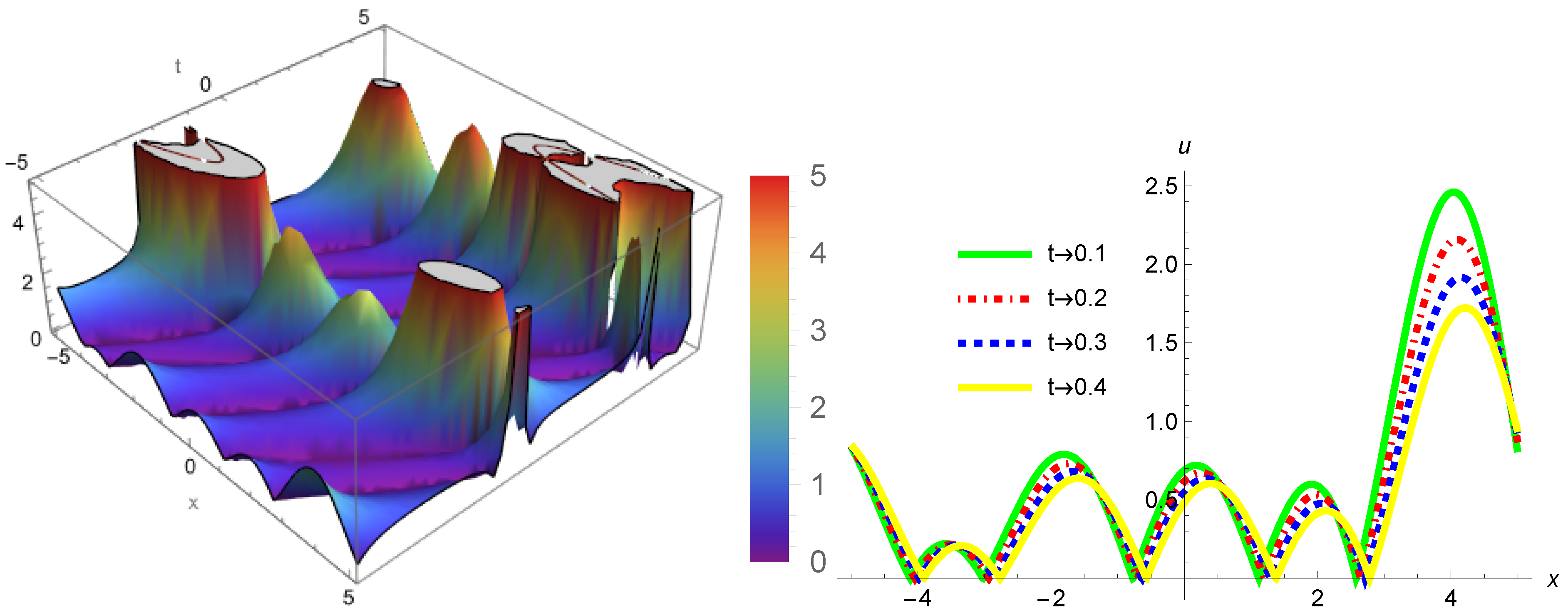
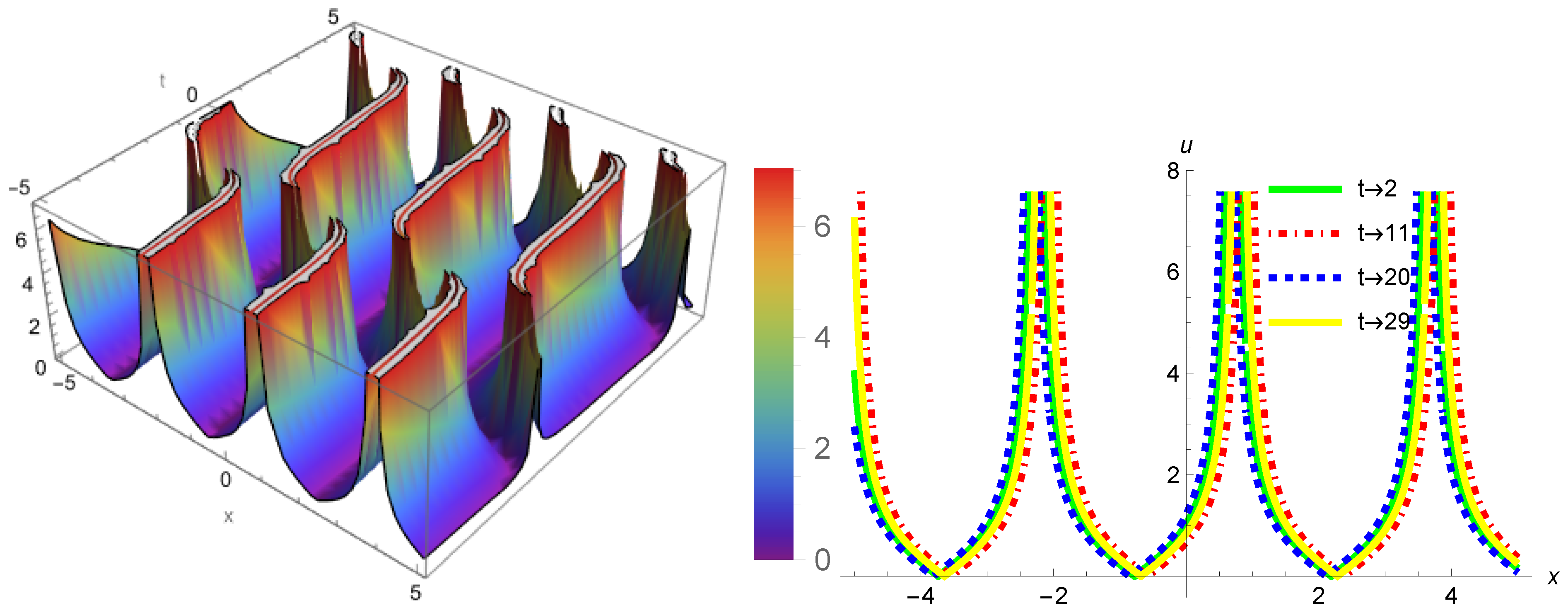
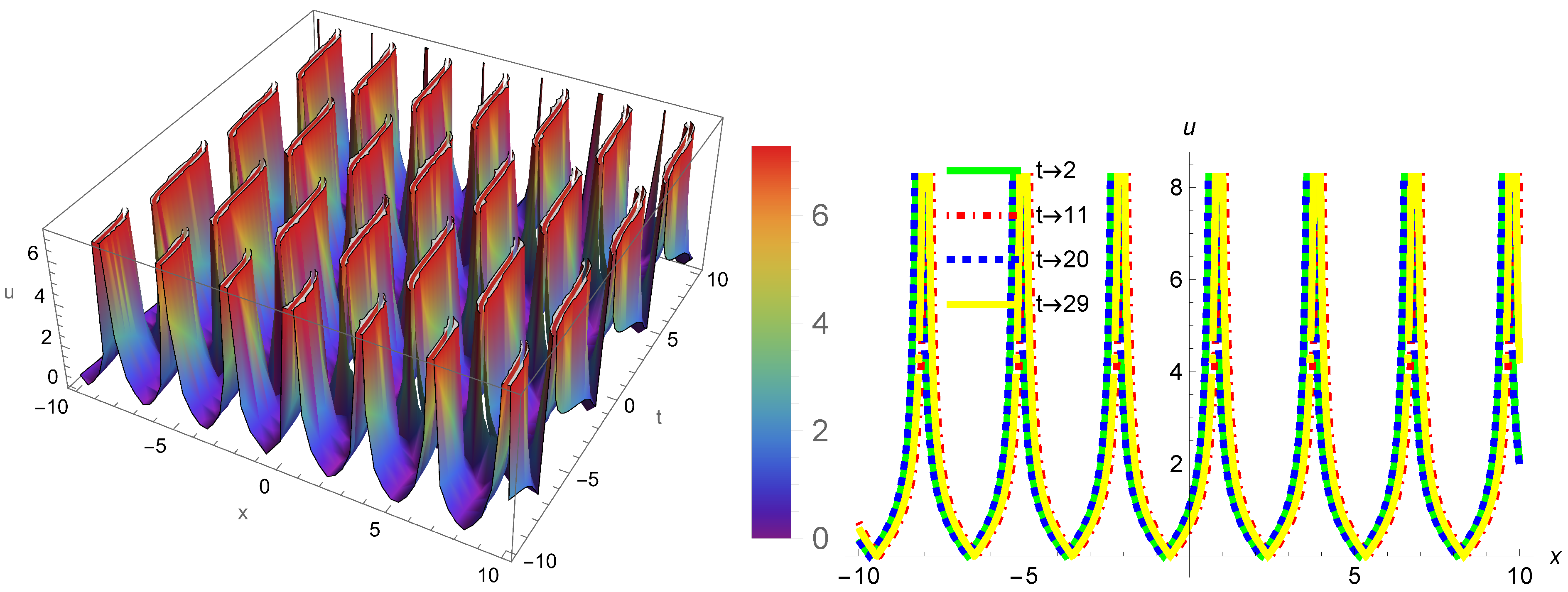
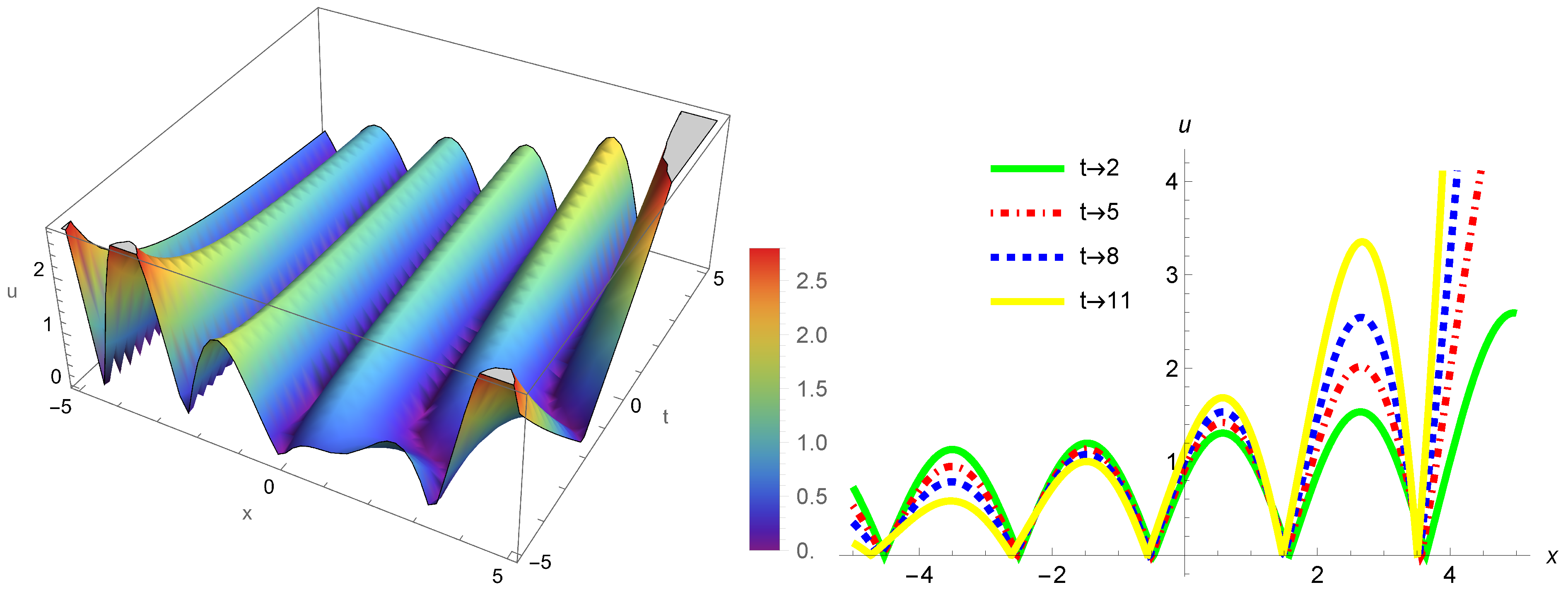
3. Physical Analysis
4. Phase Portraits and the Behavior of Bifurcations
4.1. Case 1
- , , .
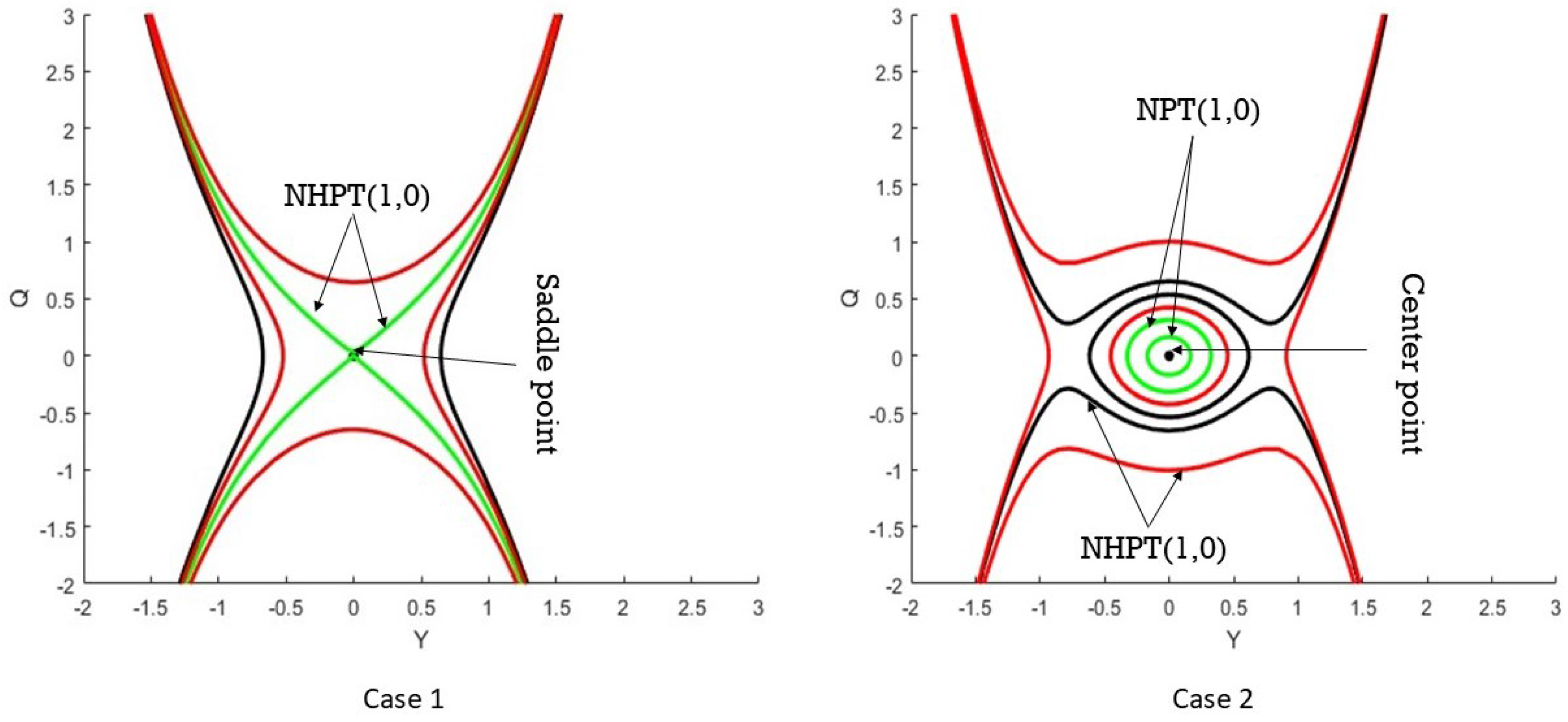
4.2. Case 2
- , , .
- , and , with . The phase portrait, shown in Figure 5, shows a center equilibrium (green and black curves), by which closed orbits (periodic) indicate stable motion and boundedness. We find these trajectories to oscillate around the equilibrium point non divergently, demonstrating that the system remains conservative. In the case of the outermost trajectories, regions are demonstrated in the phase space where the motion is still contained but does not escape to infinity, confirming the stability of the central equilibrium.
4.3. Case 3
- , , .
4.4. Case 4
- , , .
5. Chaos and Quasi-Periodic Behaviors
5.1. Quasi Periodic Oscillations
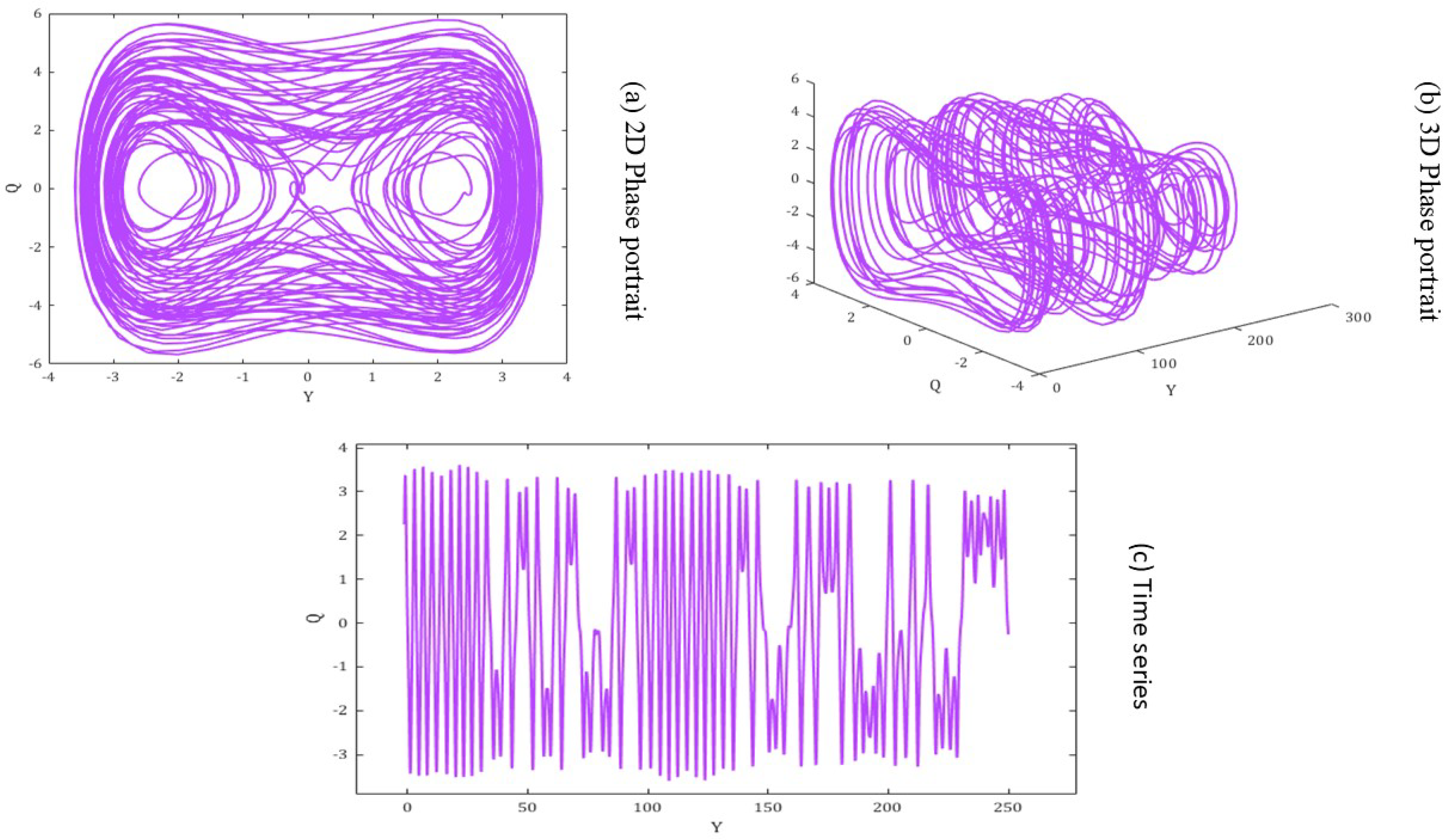
5.2. Chaotic Pattern
6. Comparison with Existing Models
- Classical integer-order models vs. fractional-order models: the traditional plasma wave models base their analysis on integer-order differential equations that use local interaction methods while having no memory features. The simplified wave behavioral representation offered by these models proves insufficient because they lack a full understanding of longer-scale correlations, together with complex wave movement patterns. The fractional-order approach includes memory-dependent terms because they enable more accurate simulations of wave propagation along with dispersion phenomena and system stability features.
- Existing chaotic wave models vs. lpd-based fractional model: most research on plasma chaos previously employed standard nonlinear Schrödinger equations as well as Ginzburg–Landau equations or Duffing-like oscillators. Periodic waveforms and solitary wave solutions match the performance of these models until they fail to capture chaotic wave behavior. Through the introduction of fractional diffusion-reaction components, the Caputo type LPD model expands previous research to enhance the characterization of plasma systems regarding their multi-stability features and periodic wave patterns and chaotic attractor dynamics.
- Comparison with perturbative and numerical methods: two main analytical tools, referred to as multiple-scale analysis and variational approaches, have traditionally been used to research wave stability patterns in plasma systems. These analysis techniques need to establish specific restrictions when studying wave phenomena. Bifurcation analysis, together with numerical simulations, allows a complete assessment of wave behavior as it depends on varying parameters, which reveals important information about stable and unstable domains.
- Phase portraits and bifurcation analysis: research on wave dynamics fails to provide organized phase analysis for visualizing how waves transform into different operating states. The systematic creation of phase diagrams through our research enables the identification of stable, periodic, and chaotic regions through system parameter assessment. The visual diagrams enhance understanding of plasma instabilities, together with nonlinear effects.
7. Conclusions
Future Developments
- Research into multi-component plasma environments using higher-dimensional plasma wave systems needs further development of the fractional-order Lakshmanan–Porsezian–Daniel (LPD) model.
- Experiments should be conducted to test computational and theoretical findings through the simulation of plasma wave phenomena under fractional-order rules.
- By adopting machine learning approaches, scientists can enhance their capability to predict plasma wave bifurcation patterns and chaotic transitions, which would benefit nonlinear wave control and optimization strategies.
- These research methods demonstrate value for advancement in different fields, primarily including nonlinear optics and quantum mechanics, as well as geophysical fluid dynamics since fractional-order models excel at evaluating long-term relationships and accumulated past responses.
- New computational approaches should be developed to enhance both the speed and accuracy of plasma wave simulations and electromagnetic wave propagation forecasts for live applications.
Author Contributions
Funding
Data Availability Statement
Conflicts of Interest
References
- Rehman, Z.U.; Zahid, M.; Bolla, D.P.; Shoaib, S.; Amin, Y.; Khattak, R.; Muddassar, M. Nonlinear wave dynamics and multistability in engineering electromagnetics: Numerical analysis of perturbed and un-perturbed systems within the Higgs field. Results Eng. 2025, 25, 104375. [Google Scholar] [CrossRef]
- Chatterjee, R. Fundamental Concepts and Discussion of Plasma Physics. TECHNO REVIEW J. Technol. Manag. 2022, 2, 1–14. [Google Scholar] [CrossRef]
- Ren, Y.; Yang, Z.Y.; Liu, C.; Yang, W.L. Different types of nonlinear localized and periodic waves in an erbium-doped fiber system. Phys. Lett. A 2015, 379, 2991–2994. [Google Scholar] [CrossRef]
- Demiray, S.T.; Bulut, H. Soliton solutions of some nonlinear evolution problems by GKM. Neural Comput. Appl. 2019, 31, 287–294. [Google Scholar] [CrossRef]
- Yang, L.; Gao, B. Solitons, kink-solitons and breather solutions of the two-coupled incoherent nonlinear Schrödinger equation. Nonlinear Dyn. 2024, 112, 5621–5633. [Google Scholar] [CrossRef]
- Ghandour, R.; Karar, A.S.; Al Barakeh, Z.; Barakat, J.; Rehman, Z. Non-Linear Plasma Wave Dynamics: Investigating Chaos in Dynamical Systems. Mathematics 2024, 12, 2958. [Google Scholar] [CrossRef]
- Shu, W.; Zhao, C.; Wen, S. Dispersion and nonlinearity in subwavelength-diameter optical fiber with high-index-contrast dielectric thin films. Proc. SPIE Int. Soc. Opt. Eng. 2010, 7846. [Google Scholar] [CrossRef]
- Singh, P.; Senthilnathan, K. Evolution of a solitary wave: Optical soliton, soliton molecule and soliton crystal. Discov. Appl. Sci. 2024, 6, 464. [Google Scholar] [CrossRef]
- Hussain, Z.; Rehman, Z.; Abbas, T.; Smida, K.; Le, Q.; Abdelmalek, Z.; Tlili, I. Analysis of bifurcation and chaos in the traveling wave solution in optical fibers using the Radhakrishnan–Kundu–Lakshmanan equation. Results Phys. 2023, 55, 107145. [Google Scholar] [CrossRef]
- Irimiciuc, S.; Saviuc, A.; Tudose-Sandu-Ville, F.; Toma, S.; Nedeff, F.; Rusu, C.; Agop, M. Non-Linear Behaviors of Transient Periodic Plasma Dynamics in a Multifractal Paradigm. Symmetry 2020, 12, 1356. [Google Scholar] [CrossRef]
- Breedt, I.; Fourie, A. The Ripple Effect: How Chaos Theory can Transform Education. Int. Conf. Educ. Res. 2024, 1, 29–35. [Google Scholar] [CrossRef]
- Ham, C.; Kirk, A.; Pamela, S.; Wilson, H. Filamentary plasma eruptions and their control on the route to fusion energy. Nat. Rev. Phys. 2020, 2, 159–167. [Google Scholar] [CrossRef]
- Ortigueira, M.; Tenreiro Machado, J. What is a fractional derivative? J. Comput. Phys. 2014, 293, 4–13. [Google Scholar] [CrossRef]
- Lazarević, M.; Rapaić, M.; Šekara, T. Introduction to Fractional Calculus with Brief Historical Background; WSEAS Press: Zografou, Greece, 2014; pp. 3–16. [Google Scholar]
- Grach, S.; Mishin, E.; Sergeev, E.; Shindin, A. Dynamic properties of ionospheric plasma turbulence driven by high-power high-frequency radiowaves. Physics-Uspekhi 2016, 59. [Google Scholar] [CrossRef]
- Tang, L.; Biswas, A.; Yildirim, Y.; Alshomrani, A. Bifurcations and optical soliton perturbation for the Lakshmanan–Porsezian–Daniel system with Kerr law of nonlinear refractive index. J. Opt. 2024. [Google Scholar] [CrossRef]
- Khelil, K.; Dekhane, A.; Benselhoub, A.; Bellucci, S. Higher order dispersions effect on high-order soliton interactions. Technol. Audit. Prod. Reserv. 2023, 2, 70. [Google Scholar] [CrossRef]
- Hamza, A.; Suhail, M.; Alsulami, A.; Mustafa, A.; Aldwoah, K.; Saber, H. Exploring Soliton Solutions and Chaotic Dynamics in the (3+1)-Dimensional Wazwaz–Benjamin–Bona–Mahony Equation: A Generalized Rational Exponential Function Approach. Fractal Fract. 2024, 8, 592. [Google Scholar] [CrossRef]
- Alraqad, T.; Suhail, M.; Saber, H.; Aldwoah, K.; Eljaneid, N.; Alsulami, A.; Muflh, B. Investigating the Dynamics of a Unidirectional Wave Model: Soliton Solutions, Bifurcation, and Chaos Analysis. Fractal Fract. 2024, 8, 672. [Google Scholar] [CrossRef]
- Zabolotnykh, A. Nonlinear Schrodinger equation for a two-dimensional plasma: The analysis of solitons, breathers, and plane wave stability. arXiv 2023, arXiv:2302.01057. [Google Scholar] [CrossRef]
- Seadawy, A.; Iqbal, M.; Lu, D. Propagation of kink and anti-kink wave solitons for the nonlinear damped modified Korteweg–de Vries equation arising in ion-acoustic wave in an unmagnetized collisional dusty plasma. Phys. A Stat. Mech. Its Appl. 2019, 544, 123560. [Google Scholar] [CrossRef]
- Bhowmike, N.; Rehman, Z.U.; Zahid, M.; Shoaib, S.; Mudassar, M. Bifurcation and multi-stability analysis of microwave engineering systems: Insights from the Burger–Fisher equation. Phys. Open 2024, 21, 100242. [Google Scholar] [CrossRef]
- Jhangeer, A.; Almusawa, H.; Hussain, Z. Bifurcation study and pattern formation analysis of a nonlinear dynamical system for chaotic behavior in traveling wave solution. Results Phys. 2022, 37, 105492. [Google Scholar] [CrossRef]
- El-Dessoky, M.; Elmandouh, A. Qualitative analysis and wave propagation for Konopelchenko-Dubrovsky equation. Alex. Eng. J. 2023, 67, 525–535. [Google Scholar] [CrossRef]
- Triki, H.; Biswas, A.; Milović, D.; Belić, M. Chirped femtosecond pulses in the higher-order nonlinear Schrödinger equation with non-Kerr nonlinear terms and cubic–quintic–septic nonlinearities. Opt. Commun. 2016, 366, 362–369. [Google Scholar] [CrossRef]
- Bohr, T.; Jensen, M.; Paladin, G.; Vulpiani, A. Dynamical Systems Approach to Turbulence; Cambridge University Press: Cambridge, UK, 2005; Volume 8. [Google Scholar] [CrossRef]
- Bibi, A.; Shakeel, M.; Khan, D.; Hussain, S.; Chou, D. Study of solitary and kink waves, stability analysis, and fractional effect in magnetized plasma. Results Phys. 2023, 44, 106166. [Google Scholar] [CrossRef]
- Kumar, M.; Mehta, U.; Cirrincione, G. A Novel Approach to Modeling Incommensurate Fractional Order Systems Using Fractional Neural Networks. Mathematics 2023, 12, 83. [Google Scholar] [CrossRef]
- Wang, M.; Li, X.; Zhang, J.L. The G′G2-expansion method and travelling wave solutions of nonlinear evolution equations in mathematical physics. Phys. Lett. A 2007, 372, 417–423. [Google Scholar] [CrossRef]
- Salinger, A.; Phipps, E.; Dijkstra, H.; Wubs, F.; Cliffe, K.; Doedel, E.; Dragomirescu, I.; Eckhardt, B.; Gelfgat, A.; Hazel, A.; et al. Numerical Bifurcation Methods and their Application to Fluid Dynamics: Analysis beyond Simulation. Commun. Comput. Phys. 2014, 15, 1–45. [Google Scholar] [CrossRef]
- Bonizzoni, G.; Vassallo, E. Plasma physics and technology; Industrial applications. Vacuum 2002, 64, 327–336. [Google Scholar] [CrossRef]


Disclaimer/Publisher’s Note: The statements, opinions and data contained in all publications are solely those of the individual author(s) and contributor(s) and not of MDPI and/or the editor(s). MDPI and/or the editor(s) disclaim responsibility for any injury to people or property resulting from any ideas, methods, instructions or products referred to in the content. |
© 2025 by the authors. Licensee MDPI, Basel, Switzerland. This article is an open access article distributed under the terms and conditions of the Creative Commons Attribution (CC BY) license (https://creativecommons.org/licenses/by/4.0/).
Share and Cite
Khan, A.G.; Muddassar, M.; Shoaib, S.; Rehman, Z.U.; Zahid, M. Dynamical Systems with Fractional Derivatives: Focus on Phase Portraits and Plasma Wave Propagation Using Lakshmanan–Porsezian–Daniel Model. Axioms 2025, 14, 405. https://doi.org/10.3390/axioms14060405
Khan AG, Muddassar M, Shoaib S, Rehman ZU, Zahid M. Dynamical Systems with Fractional Derivatives: Focus on Phase Portraits and Plasma Wave Propagation Using Lakshmanan–Porsezian–Daniel Model. Axioms. 2025; 14(6):405. https://doi.org/10.3390/axioms14060405
Chicago/Turabian StyleKhan, Abdul Ghaffar, Muhammad Muddassar, Sultan Shoaib, Zia Ur Rehman, and Muhammad Zahid. 2025. "Dynamical Systems with Fractional Derivatives: Focus on Phase Portraits and Plasma Wave Propagation Using Lakshmanan–Porsezian–Daniel Model" Axioms 14, no. 6: 405. https://doi.org/10.3390/axioms14060405
APA StyleKhan, A. G., Muddassar, M., Shoaib, S., Rehman, Z. U., & Zahid, M. (2025). Dynamical Systems with Fractional Derivatives: Focus on Phase Portraits and Plasma Wave Propagation Using Lakshmanan–Porsezian–Daniel Model. Axioms, 14(6), 405. https://doi.org/10.3390/axioms14060405