Stabilization and Synchronization of a New 3D Complex Chaotic System via Adaptive and Active Control Methods

Abstract

This paper investigates the controllability and synchronization of a newly designed three-dimensional chaotic system using active and adaptive control strategies. Although both controllers were designed with the help of a positive definite function using Lyapunov theory, for adaptive controllers, we estimated an unknown parameter of the system in real time and adjusted the control signal accordingly to maintain stability. Moreover, numerical simulations demonstrated that the active control approach achieved stability for both equilibrium points ($p_1$ and $p_2$) approximately at time t = $0.5$ s, demonstrating its rapid convergence and robust performance. In contrast, the adaptive control method stabilized $p_1$ at approximately $t\approx 0.5$ and $p_2$ at $t\approx 1$ s, illustrating reaching their desired conditions. Furthermore, the considered methods could effectively synchronize two identical chaotic systems, where the slave system overlapped the master system at approximately $t=5$ s. Apart from this, a detailed comparative analysis of the two techniques in terms of controllability and synchronization is presented. Moreover, the complementary strengths of these methods provide valuable perspectives for broader applications in chaotic system management and security-critical systems.

1. Introduction

Chaotic systems have gained significant attention in recent years due to their unique property, i.e., sensitivity to initial conditions (ICs), where negligible variation in their ICs of any given dynamical system can lead to substantial divergence, resulting in unpredictability and randomness. There are several potential applications of such systems in various fields, including robotics [1,2], secure communication [3,4], multi-wings/scrolls [5,6], biological sciences [7,8], engineering [9], and quantum optics [10], as also indicated in the references therein. There are several situations where the consequences of chaos in dynamical systems can lead to destruction, and negligence can cause the engulfing of several precious lives. Hence, control is vital in implementing and achieving stability before hazardous effects in such situations.

Several control techniques have been designed so far, but the sliding mode control (SMC) technique [11,12] is considered one of the first controllers designed for the said purpose. The limitation of SMC, the chattering effect in control trajectories before achieving the reaching condition, has forced researchers to design another technique to mitigate their chattering effect. Therefore, an adaptive controller was designed based on unknown parameters; this technique is applied in chaotic systems when certain parameters are unknown or need to be estimated during operation [13]. Adaptive control is a technique in which a control law is designed to update uncertain parameters in a slave chaotic system with respect to a master system, enabling synchronization between two identical chaotic systems. This approach ensures that the slave system adapts its parameters in real time to follow [14]. This technique is found in several applications for controlling chaos and achieving the desired result of easily reaching conditions. In 2019, Marwan et al. [15] considered the Rucklidge chaotic system and controlled its unpredictable attitude using three techniques, including adaptive ones. Yu et al. advanced the classical adaptive controller method by combining it with the finite-time controller input [16] to stabilize their considered system in the presence of control gains. By contrast, regarding second-order systems, their applications were reviewed in [17]. The presented approaches are used not only in chaotic systems but also in less chaotic or even nonchaotic dynamic systems, such as closed-chain mechanisms [18]. Furthermore, recent research in robotics and control indicates that machine learning-based adaptive controllers, such as reinforcement learning and neural networks, are interesting alternatives [19,20]. These data-driven approaches may outperform traditional adaptive controllers in high-dimensional or uncertain environments [21]. However, they require a large amount of training data and, in many situations, lack formal guarantees of stability [22]. Incorporating and assessing ML-based controllers remains an opportunity for future work.

Another control technique, the active control technique [23], can consider two sub-controllers simultaneously to achieve stability in a given system. Active control is widely recognized for its effectiveness in stabilizing and synchronizing chaotic systems [24,25,26]. Active control is a control technique used to synchronize chaotic systems, whether identical or nonidentical, by designing linear controllers based on known system nonlinearities, without requiring system derivatives or Lyapunov exponents, making it efficient and practical for real-world applications [27]. In [28], the authors applied an active control method to achieve chaos synchronization of their newly proposed fractional-order 3D chaotic system, enabling its use in secure audio signal transmission. In 2023, Taramim et al. [29] utilized an active controller that offered a strong foundation for addressing the challenges caused by chaotic behavior, particularly in synchronizing nonidentical chaotic systems [30].

There is another phenomenon, synchronization, working on the same rule of controllers, where the trajectory of one dynamical system (slave) overlaps another (master) system and starts following it. This concept was first described by Pecora et al. in 1990 and 1991 [31,32]. Since then, several researchers have adapted the same methodology using other control techniques, including [33,34,35,36]. In 2020, Marwan et al. [37] used an adaptive control technique to ensure global stability and achieve synchronization. The adaptive control technique was combined with a sliding controller [38] to enhance the synchronization approach and reduce the chattering effect in SMC.

In the literature, the active control method showed efficient results in suppressing chaos, and beyond stabilization, the synchronization of chaotic systems is also an integral part that can be achieved using an active controller. Moreover, the active control technique has been used in several real-life and technology-based applications, such as in secure communication, where synchronizing two identical/nonidentical chaotic systems enables encryption and decryption processes [39,40].

Chaotic systems have garnered significant attention due to their potential applications in cryptography [4], robotics [1,2], and secure communication [3]. The study of novel chaotic systems not only advances our understanding of nonlinear dynamics but also enhances control strategies for complex systems. In this work, we investigated the synchronization and controllability of a newly introduced 3D chaotic system, originally proposed by [41]. This system exhibits high complexity, with a maximal Lyapunov exponent of 7.196, and is capable of generating self-excited chaotic attractors, making it both theoretically intriguing and practically significant. While its potential for cryptography has been suggested, its full range of applications remains an open area of exploration. Furthermore, the system has been validated through circuit design, confirming its feasibility for experimental and engineering applications. Given the importance of chaos-based techniques in security and control, analyzing the stability and synchronization properties of this system provides valuable insights for future real-world implementations. By employing this system, our study contributes to the broader understanding and management of complex chaotic behaviors, offering a robust framework for the development of advanced control strategies such as active and adaptive control.

In this study, we investigated the stabilization and synchronization of chaotic systems using two distinct control strategies: active control and adaptive control. Both methods have been widely applied to chaotic and nonlinear systems, but they differ in their approach and advantages, especially when applied to complex, recently introduced chaotic systems. Active control is commonly used for synchronizing dynamical systems, particularly in mechanical models. For example, Ref. [42] analyzed how control gains influence damping and inertia, while [43] explored its integration with a predefined PID scheme to manage vibration risks. In contrast, adaptive control is particularly beneficial for systems with uncertain or varying parameters, as it continuously adjusts based on system behavior. This adaptability makes it suitable for applications like robotic systems, as demonstrated by [44], who improved stability in a snake robotic system. Similarly, Ref. [45] combined adaptive and sliding-mode control for hydraulic systems, and [46] applied it in cooperative transportation. While both methods contribute to stability, adaptive control is more effective in handling unknown parameters, whereas active control offers a more direct synchronization mechanism. Due to the special dynamic aspects of the chaotic system studied in this work, such as a high Lyapunov exponent and complex attractor structures, strong and proven control mechanisms were required for stabilization and synchronization. Each approach was applied separately to assess its effectiveness in managing chaotic dynamics. By applying both active and adaptive control methods, we aimed to evaluate their performance in stabilizing and synchronizing the chaotic system. The results were then compared to determine the strengths and limitations of each method, providing valuable insights into their respective capabilities for controlling chaotic dynamics. Using Lyapunov theory, we established global stability at the system’s equilibrium points, confirming that the proposed control techniques effectively stabilize and synchronize the chaotic system. Numerical simulations validated the performance of these nonlinear control methods in stabilizing and synchronizing complex chaotic systems.

This paper is organized as follows: Section 2 presents the problem formulation, including the mathematical model of the 3D chaotic system and its steady-state solutions. Section 3 focuses on the stabilization of the chaotic system using active and adaptive control techniques, along with a discussion of the results. Section 4 addresses the synchronization of the chaotic system, detailing the application of both control strategies and a comprehensive analysis of the outcomes. Finally, Section 5 concludes the paper, summarizing the findings and suggesting potential directions for future research.

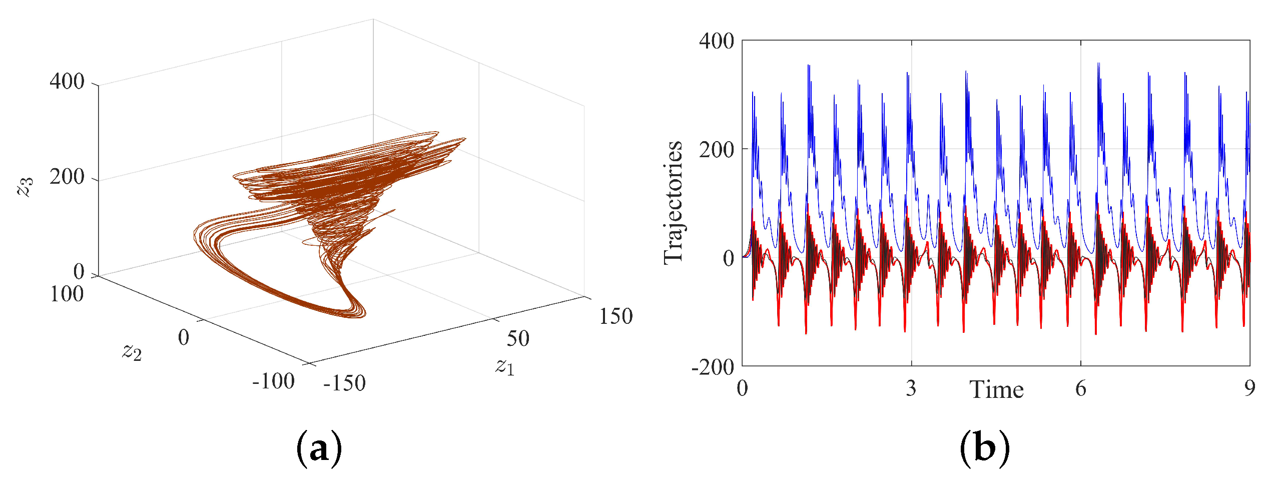
2. The 3D Chaotic System and Its Equilibrium Points

In this study, we examined a nonlinear dynamical system described by autonomous three-dimensional differential equations, as outlined in [41]:

$$\begin{array}{cc}\hfill \dot{z_1}& =\alpha (z_2-z_1)+z_2{z}_3,\hfill \\ \hfill \dot{z_2}& =z_1(\beta -z_3)-1,\hfill \\ \hfill \dot{z_3}& =z_1^2+z_1{z}_3-\gamma z_3,\hfill \end{array}$$

(1)

where $z_1$, $z_2$, and $z_3$ are the state variables, and $\alpha$, $\beta$, and $\gamma$ are parameters. System (1) is characterized by four quadratic nonlinear terms that can help generate chaotic trajectories, including self-excited chaotic attractors. Furthermore, the system has two equilibrium points that are locally saddle-foci and globally play a significant role in generating chaos. Moreover, before applying control strategies, it is essential to understand the dynamics of the system through its phase portraits and time series. In the presence of all involved parameters, system (1) exhibited no equilibrium points and hence the numerical approach was used to find their equilibrium points, i.e., $p_1$ = ($-58.5585,-16.7269,50.0171$) and $p_2$ = ($8.5385,2.4437,49.8829$), as shown in [41]. The local dynamical analysis using the Jacobian matrix and its eigenvalues shows that both equilibrium points are unstable.

In Figure 1, system (1) shows unpredictability and can be obtained for initial conditions ($z_1$, $z_2$, $z_3$) = (1, 1, 1) and parameter values $\alpha$ = 50, $\beta$ = 20, and $\gamma$ = 10. Our objective was to apply control strategies that stabilize the system and synchronize two identical chaotic systems (master and slave). To achieve this, we employed two control approaches: active and adaptive control. We aimed to design effective control laws to stabilize the considered system towards its equilibrium points and achieve synchronization between the master and slave systems. The phase portraits and time series provided in this section are reproduced to analyze and visually demonstrate the system’s chaotic behavior. This representation serves as a foundation for the control techniques in the subsequent sections.

3. Stability Analysis of the 3D Chaotic System

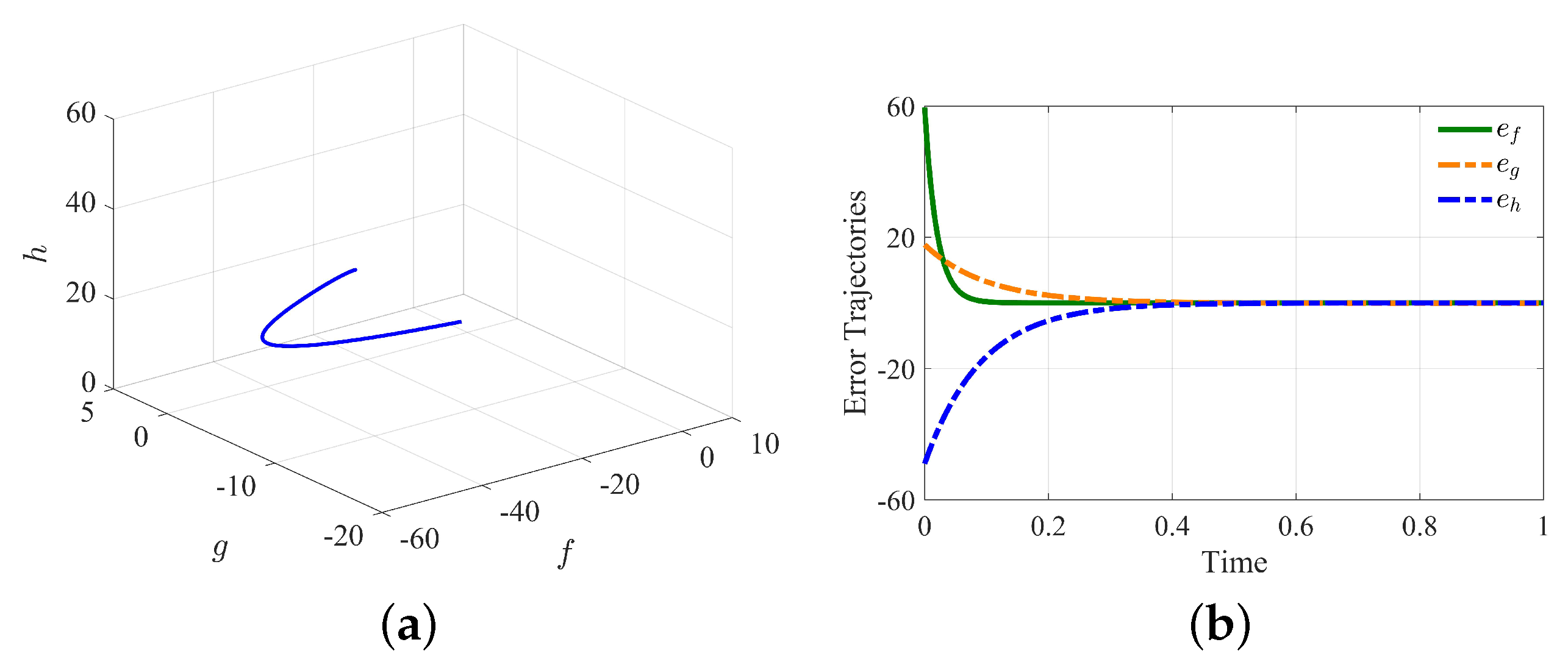
This section describes the stability analysis of the chaotic system described in Section 2, employing two distinct techniques: active control and adaptive control. We aimed to determine the closed-loop systems of the chaotic (open-loop) system using these two control approaches.

3.1. Active Control

In this subsection, we present an active controller to discuss the stability of system (1). To enhance clarity and avoid confusion, the variables $z_1$, $z_2$, and $z_3$ were replaced with f, g, and h, respectively, to obtain

$$\begin{array}{cc}\hfill \dot{f}& =\alpha (g-f)+gh,\hfill \\ \hfill \dot{g}& =f(\beta -h)-1,\hfill \\ \hfill \dot{h}& =f^2+fh-\gamma h.\hfill \end{array}$$

(2)

In the active control technique, the controller is separated further into two controllers, i.e., linear and nonlinear. The controlled system can be rewritten as

$$\begin{array}{cc}\hfill \dot{f}& =\alpha (g-f)+gh+u_1,\hfill \\ \hfill \dot{g}& =f(\beta -h)-1+u_2,\hfill \\ \hfill \dot{h}& =f^2+fh-\gamma h+u_3.\hfill \end{array}$$

(3)

The error terms $e_f=f-z_1^{*}$, $e_g=g-z_2^{*}$ and $e_h=h-z_3^{*}$ are differentiated to obtain the error dynamical system as follows:

$$\begin{array}{cc}\hfill {\dot{e}}_f& =\alpha ((e_g+z_2^{*})-(e_f+z_1^{*}))+(e_g+z_2^{*})(e_h+z_3^{*})+u_1,\hfill \\ \hfill {\dot{e}}_g& =(e_f+z_1^{*})(\beta -(e_h+z_3^{*}))-1+u_2,\hfill \\ \hfill {\dot{e}}_h& ={(e_f+z_1^{*})}^2+(e_f+z_1^{*})(e_h+z_3^{*})-\gamma (e_h+z_3^{*})+u_3.\hfill \end{array}$$

(4)

In the context of active control, the control inputs are formulated as $u_i=A_i+N_i$, where $A_i$ represents the linear components and $N_i$ denotes the nonlinear elements for $i=1,2,3$. Decomposing the control inputs into linear and nonlinear parts allows for a deeper understanding of the system dynamics and facilitates effective control strategy design. In view of Equation (4), In view of Equation (4), the controller for nonlinear terms is designed and presented in Equation (5), which is specifically formulated to cancel out the nonlinear components in the error dynamics as part of the active controller design

$$\begin{array}{cc}\hfill N_1& =-\alpha z_2^{*}+\alpha z_1^{*}-(e_g+z_2^{*})(e_h+z_3^{*}),\hfill \\ \hfill N_2& =-\beta z_1^{*}+(e_f+z_1^{*})(e_h+z_3^{*}),\hfill \\ \hfill N_3& =-{(e_h+z_1^{*})}^2-(e_f+z_1^{*})(e_h+z_3^{*})+\gamma z_3^{*}.\hfill \end{array}$$

(5)

Substituting Equation (5) into Equation (4), we obtain

$$\begin{array}{cc}\hfill {\dot{e}}_f& =\alpha e_g-\alpha e_f+A_1,\hfill \\ \hfill {\dot{e}}_g& =\beta e_f-1+A_2,\hfill \\ \hfill {\dot{e}}_h& =-\gamma e_h+A_3,\hfill \end{array}$$

(6)

where we put Equation (7) results from designing a linear error feedback controller to stabilize the remaining linear part of the dynamics

$$\begin{array}{cc}\hfill \left[\begin{array}{c}{A}_1\\ A_2\\ A_3\end{array}\right]& =\left[\begin{array}{ccc}-k_1& -\alpha & 0\\ -\beta & -k_2& 0\\ 0& 0& -k_3\end{array}\right]\left[\begin{array}{c}{e}_f\\ e_g\\ e_h\end{array}\right].\hfill \end{array}$$

(7)

Thus, resubstituting Equations (5) and (7) into Equation (4), we obtain the final closed-loop system with active controllers as follows:

$$\begin{array}{cc}\hfill {\dot{e}}_f& =-\alpha e_f-k_1{e}_f,\hfill \\ \hfill {\dot{e}}_g& =-1-k_2{e}_g,\hfill \\ \hfill {\dot{e}}_h& =-\gamma e_h-k_3{e}_h.\hfill \end{array}$$

(8)

Finally, to validate the reaching condition of the designed controller, we considered a positive definite Lyapunov function

$$\begin{array}{c}\hfill V_1={\displaystyle \frac{1}{2}}(e_f^2+e_g^2+e_h^2)\end{array}$$

(9)

was considered. Equation (9) is the sum of the square of each term, and it can be easily proved that $V_1$ is non-negative. Moreover, the next step is to demonstrate the negative definiteness of its derivative. Hence, differentiating $V_1$ and substituting back Equation (5) into it, we obtain the following:

$$\begin{array}{c}\hfill {\dot{V}}_1=-(\alpha +k_1)e_f^2-k_2{e}_g^2-(\gamma +k_3)e_h^2-e_g.\end{array}$$

(10)

The negative definiteness of ${\dot{V}}_1$ confirms the desired outcome. Additionally, active control enables the system to stabilize toward the equilibrium points $p_1$ and $p_2$.

3.2. Adaptive Control

In this subsection, the chaos control of our considered dynamical system (1) is attained by employing an adaptive control strategy. Subsequently, to effectively govern the 3D chaotic system characterized by entirely unknown parameters, in this context, we introduce adaptive control signals, denoted as $w_1$, $w_2$, and $w_3$, to stabilize the chaos. In this work, we assumed that only the parameter $\alpha$ is unknown. The other system parameters, $\beta$ and $\gamma$, were assumed to be known and constant throughout the control process.

The primary objective of the adaptive controller is to generate control signals, specifically $w_1$, $w_2$, and $w_3$, to mitigate the inherent nonlinearity. The target of this controller was to dissipate the linear system, particularly characterized by equilibrium points. To accomplish this objective, the control inputs $w_1$, $w_2$, and $w_3$ were added in system (1):

$$\begin{array}{cc}\hfill {\dot{z}}_1& =\alpha (z_2-z_1)+z_2{z}_3+w_1,\hfill \\ \hfill {\dot{z}}_2& =z_1(\beta -z_3)-1+w_2,\hfill \\ \hfill {\dot{z}}_3& =z_1^2+z_1{z}_3-\gamma z_3+w_3.\hfill \end{array}$$

(11)

Utilizing error terms as outlined in Section 3.1, we derived the error dynamical system as

$$\begin{array}{cc}\hfill {\dot{e}}_1& =\alpha (e_2-e_1+z_2^{*}-z_1^{*})+(e_2+z_2^{*})(e_3+z_3^{*})+w_1,\hfill \\ \hfill {\dot{e}}_2& =(e_1+z_1^{*})(\beta -(e_3+z_3^{*}))-1+w_2,\hfill \\ \hfill {\dot{e}}_3& ={(e_1+z_1^{*})}^2+(e_1+z_1^{*})(e_3+z_3^{*})-\gamma (e_3+z_3^{*})+w_3.\hfill \end{array}$$

(12)

Given Equation (12), we obtained the control input as

$$\begin{array}{cc}\hfill w_1& =-\widehat{\alpha }(e_2-e_1+z_2^{*}-z_1^{*})-(e_2+z_2^{*})(e_3+z_3^{*})-k_4{e}_1,\hfill \\ \hfill w_2& =-\beta (e_1+z_1^{*})+(e_1+z_1^{*})(e_3+z_3^{*})-k_5{e}_2,\hfill \\ \hfill w_3& =-{(e_1+z_1^{*})}^2-(e_1+z_1^{*})(e_3+z_3^{*})+\gamma z_3^{*}-k_6{e}_3,\hfill \end{array}$$

(13)

where $\widehat{\alpha }$ is the estimated parameter of $\alpha$ and is completely unknown; the additional constants $k_4$, $k_5$, and $k_6$ are positive gain elements. The error between the estimated and true value of the system’s parameter $\alpha$ is $e_{\alpha }=\alpha -\widehat{\alpha }$, serving as an approximation derived from the estimation process (time-dependent) rather than the true value. Although it is possible to treat other parameters as unknown, in this study, only $\alpha$ was treated adaptively to highlight its critical role in controlling chaotic behavior. Substituting Equation (13) back into Equation (12), we obtain

$$\begin{array}{cc}\hfill {\dot{e}}_1& =e_{\alpha }\left(e_2-e_1+z_2^{*}-z_1^{*}\right)-k_4{e}_1,\hfill \\ \hfill {\dot{e}}_2& =-1-k_5{e}_2,\hfill \\ \hfill {\dot{e}}_3& =-(\gamma +k_6)e_3.\hfill \end{array}$$

(14)

To formulate the control law enabling the refinement of parameter estimates, we established the Lyapunov positive definite function $V_2(e_a,e_b,e_c,e_{\alpha })$ for the controlled chaotic system described by Equation (14) as follows:

$$\begin{array}{c}\hfill V_2={\displaystyle \frac{1}{2}}(e_1^2+e_2^2+e_3^2+e_{\alpha }^2).\end{array}$$

(15)

The choice of the Lyapunov function (15) ensures its positivity in ${\mathbb{R}}^4$, implying the positive definiteness of $V_2$. To establish the negative definiteness of ${\dot{V}}_2$, we computed the time derivative of $V_2$ with respect to time and substituted Equation (14) into it to obtain the following result:

$$\begin{array}{c}\hfill {\dot{V}}_2=e_1{e}_{\alpha }\left(e_2-e_1+z_2^{*}-z_1^{*}\right)-k_4{e}_1^2\\ \hfill -e_2(1+k_5{e}_2)-(\gamma +k_6)e_3^2-e_{\alpha }\dot{\widehat{\alpha }}.\end{array}$$

(16)

The functions governing $\dot{\widehat{\alpha }}$, ensuring the negativity of ${\dot{V}}_2$, can be derived by employing Equation (15) into Equation (16), establishing the following relationship:

$$\begin{array}{c}\hfill \dot{\widehat{\alpha }}=e_1\left(e_2-e_1+z_2^{*}-z_1^{*}\right)+k_7{e}_{\alpha },\end{array}$$

(17)

where $k_7$ is a positive constant. Now, consider the new Lyapunov function, denoted as $V_3$, defined as $V_3=V_2+{\displaystyle \frac{1}{2}}{e}_{\alpha }^2$. Upon substituting Equations (16) and (17) into $V_3$, we obtain its derivative as

$$\begin{array}{cc}\hfill {\dot{V}}_3& =-k_4{e}_1^2-k_5{e}_2^2-(\gamma +k_6)e_3^2-k_7{e}_{\alpha }^2-e_2.\hfill \end{array}$$

(18)

$V_3$ confirms that system (1) in the presence of control inputs and updated law is controlled.

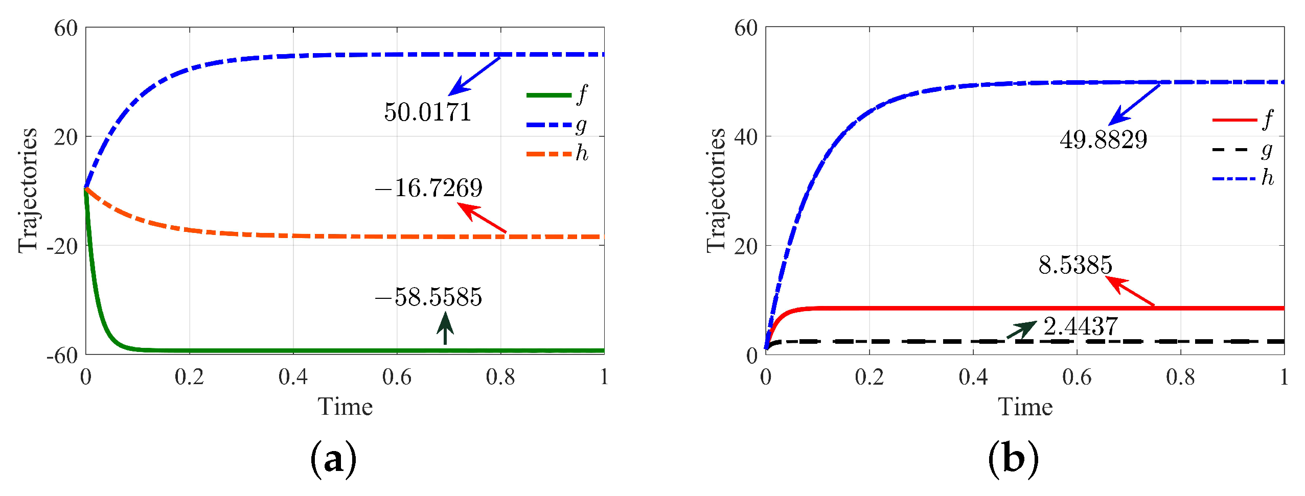
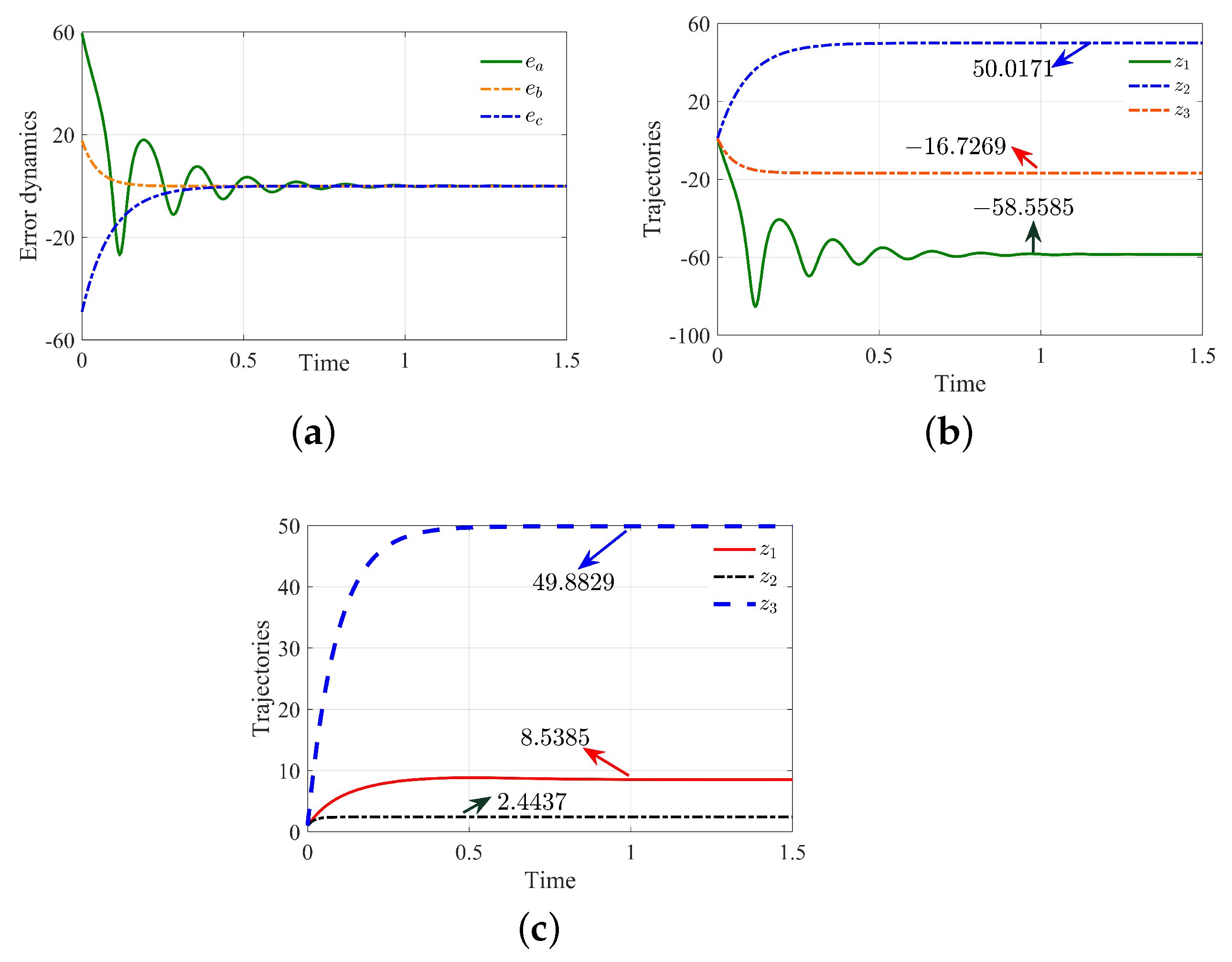
3.3. Stability: Results and Discussion

The stabilization of the 3D chaotic system under active and adaptive control techniques demonstrates the efficacy of these approaches in directing chaotic dynamics toward desired equilibrium points.

For the active control technique, the phase portraits in Figure 2a show the system’s trajectories stabilizing at equilibrium points $p_1$ (left) and $p_2$ (right), confirming the method’s effectiveness. The error dynamics presented in Figure 2b exhibit a rapid convergence to zero around $t\approx 0.5$ s, emphasizing the precision of this technique. Additionally, Figure 3 highlights the time history of the state variables, with trajectories steadily converging toward the equilibrium points $p_1$ and $p_2$, respectively.

Figure 4a illustrates phase portraits with trajectories converging to equilibrium points $p_1$ and $p_2$ using an adaptive control technique. In contrast, in Figure 4b, the updated law/parameter estimation dynamics during the control process can be observed, which is also useful in system adjustments by tuning the parameters. The error dynamics in Figure 5a demonstrate the convergence to zero at $t=1$ and $t=0.5$ s for both equilibrium points, respectively. Furthermore, Figure 5b,c depict the time history of state variables, showing the systems’ stabilization with respect to time, especially toward the specified equilibrium points.

The comparative analysis of these techniques reveals that although both effectively stabilize the chaotic system, active control input offers rapid and uniform stabilization. In contrast, adaptive control demonstrates flexibility in managing parameter variations. Together, they highlight a robust approach to stabilizing chaotic systems, ensuring stability and reliability in diverse scenarios.

4. Synchronization of the 3D Chaotic System

Synchronization plays a crucial role in stabilizing chaotic systems, ensuring accurate control and behavior [47]. For instance, in secure communication, synchronization between master and slave systems is essential for reliable transmission and decryption of messages. The system utilized here has also been suggested to be highly effective for securing communication, as highlighted in the work of [41].

4.1. Active Control Synchronization

We consider system (1) as the plant system for identical synchronization using an active controller. For this purpose, system (1) is transformed with the change in variables to $y_1$, $y_2$, and $y_3$, for instance,

$$\begin{array}{cc}\hfill {\dot{y}}_1& =\alpha (y_2-y_1)+y_2{y}_3+u_4,\hfill \\ \hfill {\dot{y}}_2& =y_1(\beta -y_3)-1+u_5,\hfill \\ \hfill {\dot{y}}_3& =y_1^2+y_1{y}_3-\gamma y_1+u_6,\hfill \end{array}$$

(19)

where $u_4$, $u_5$, and $u_6$ are control inputs that will be determined later using an active controller. First, the error terms

$$\begin{array}{cc}\hfill e_1& =y_1-f,\hfill \\ \hfill e_2& =y_2-g,\hfill \\ \hfill e_3& =y_3-h,\hfill \end{array}$$

(20)

are differentiated to obtain the error dynamical system

$$\begin{array}{cc}\hfill {\dot{e}}_1& =\alpha e_2-\alpha e_1+y_2{y}_3-gh+u_4,\hfill \\ \hfill {\dot{e}}_2& =\beta e_1-y_1{y}_3+fh+u_5,\hfill \\ \hfill {\dot{e}}_3& =y_1^2-f^2+y_1{y}_3-fh-\gamma e_3+u_6,\hfill \end{array}$$

(21)

which is used for synchronization and work under the rule that as error terms approach zero, the trajectories of the slave system will overlap with their corresponding master system. Similar to the concept used for controlling chaos in Section 3.1, the control input $u_i=A_i+N_i$ is divided into nonlinear and linear components. The nonlinear terms are as follows:

$$\begin{array}{cc}\hfill N_4& =-y_2{y}_3+gh,\hfill \\ \hfill N_5& =y_1{y}_3-fh,\hfill \\ \hfill N_6& =-y_1^2+f^2-y_1{y}_3+fh.\hfill \end{array}$$

(22)

Substituting Equation (22) into Equation (21), we obtain

$$\begin{array}{cc}\hfill {\dot{e}}_f& =\alpha e_2-\alpha e_1+A_4,\hfill \\ \hfill {\dot{e}}_g& =\beta e_1+A_5,\hfill \\ \hfill {\dot{e}}_h& =-\gamma e_3+A_6,\hfill \end{array}$$

(23)

where

$$\begin{array}{cc}\hfill \left[\begin{array}{c}{A}_4\\ A_5\\ A_6\end{array}\right]& =\left[\begin{array}{ccc}-k_1& -\alpha & 0\\ -\beta & -k_2& 0\\ 0& 0& -k_3\end{array}\right]\left[\begin{array}{c}{e}_1\\ e_2\\ e_3\end{array}\right].\hfill \end{array}$$

(24)

To design the active synchronization mechanism, we modified the system behavior by incorporating the linear and nonlinear control components. The modified error dynamics are

$$\begin{array}{cc}\hfill {\dot{e}}_1& =-\alpha e_1-k_8{e}_1,\hfill \\ \hfill {\dot{e}}_2& =-k_9{e}_2,\hfill \\ \hfill {\dot{e}}_3& =-\gamma e_3-k_{10}{e}_3.\hfill \end{array}$$

(25)

To prove the stability of the synchronization, we selected a positive definite Lyapunov function

$$\begin{array}{c}\hfill V_4={\displaystyle \frac{1}{2}}(e_1^2+e_2^2+e_3^2),\end{array}$$

(26)

such that its derivative

$$\begin{array}{c}\hfill {\dot{V}}_4=-(\alpha +k_8)e_1^2-k_9{e}_2^2-(\gamma +k_{10})e_3^2\end{array}$$

(27)

is negative definite. The expression for ${\dot{V}}_4$ is negative, indicating that the error terms converge to zero, ensuring the synchronization of the slave system with the master system.

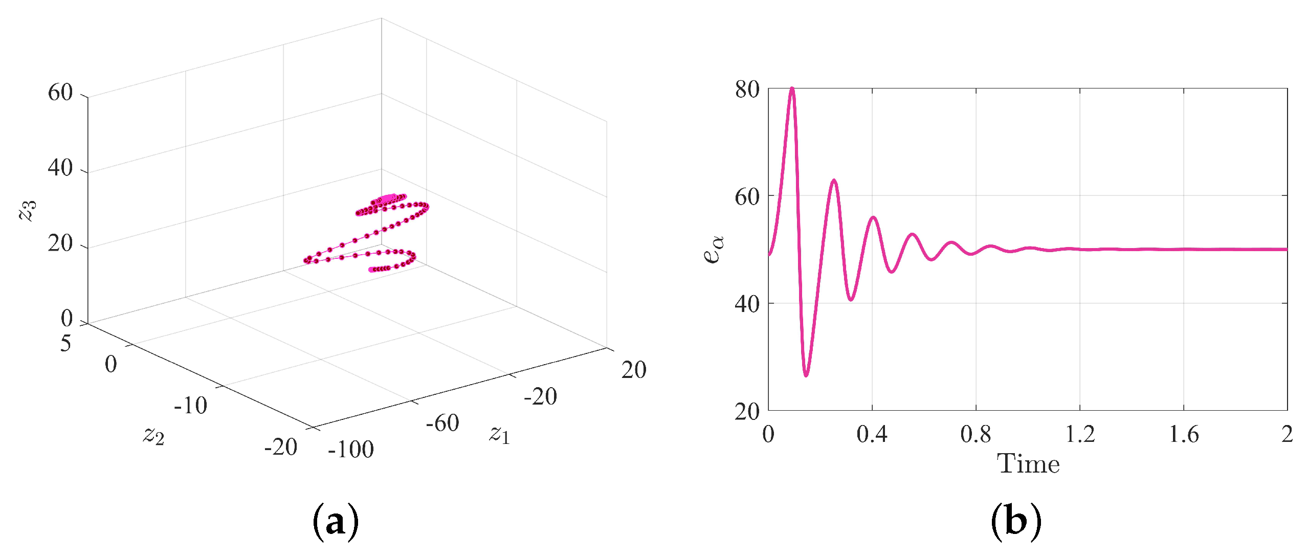
4.2. Adaptive Synchronization

Similar to the concept of active synchronization, we consider system (1) as master and consider the same as slave for adaptive synchronization. The following error dynamical system is obtained:

$$\begin{array}{cc}\hfill {\dot{e}}_4& =\alpha e_5-\alpha e_4+y_2{y}_3-z_2{z}_3+w_4,\hfill \\ \hfill {\dot{e}}_5& =\beta e_4-y_1{y}_3+z_1{z}_3+w_5,\hfill \\ \hfill {\dot{e}}_6& =y_1^2-z_1^2+y_1{y}_3-z_1{z}_3-\gamma e_6+w_6.\hfill \end{array}$$

(28)

Consequently, the adaptive synchronization inputs $w_i$ are defined as

$$\begin{array}{cc}\hfill w_4& =-\widehat{\alpha }(e_5-e_4)-y_2{y}_3+z_2{z}_3-k_{11}{e}_4,\hfill \\ \hfill w_5& =y_1{y}_3-z_1{z}_3-k_{12}{e}_5,\hfill \\ \hfill w_6& =-y_1^2+z_1^2-y_1{y}_3+z_1{z}_3-k_{13}{e}_6,\hfill \end{array}$$

(29)

where $e_{\alpha }=\alpha -\widehat{\alpha }$. Substituting Equation (29) into (28) yields the following:

$$\begin{array}{cc}\hfill {\dot{e}}_4& =e_{\alpha }(e_5-e_4)-k_{11}{e}_4,\hfill \\ \hfill {\dot{e}}_5& =\beta e_4-k_{12}{e}_5,\hfill \\ \hfill {\dot{e}}_6& =-\gamma e_6-k_{13}{e}_6,\hfill \end{array}$$

(30)

where $k_{11}$, $k_{12}$, and $k_{13}$ are positive constants. To formulate the control law for refining parameter estimates, we established the Lyapunov positive definite function $V_2(e_a,e_b,e_c,e_{\alpha })$ for the controlled chaotic system described by Equation (14) as follows:

$$\begin{array}{c}\hfill V_5={\displaystyle \frac{1}{2}}(e_4^2+e_5^2+e_6^2+e_{\alpha }^2).\end{array}$$

(31)

The quadratic Lyapunov function in Equation (31) ensures positivity over ${\mathbb{R}}^4$, implying the positive definiteness of $V_5$. To establish the negative definiteness of $\dot{V_5}$, we computed the time derivative of $V_5$ with respect to time:

$$\begin{array}{c}\hfill {\dot{V}}_5=e_{\alpha }(e_4{e}_5-e_4^2-k_{11}{e}_4^2-\dot{\widehat{\alpha }})+e_5(\beta -k_{12}{e}_5)\\ \hfill +e_6(-\gamma e_6-k_{13}{e}_6)+e_{\alpha }{\dot{e}}_{\alpha }.\end{array}$$

(32)

To make $\dot{V_5}$ negative definite, we select $k_{12}>20$ and

$$\begin{array}{c}\hfill {\dot{e}}_{\alpha }=e_4{e}_5-e_4^2-k_{11}{e}_4^2-k_{14}{e}_{\alpha }.\end{array}$$

(33)

Substituting Equation (33) into Equation (32), we obtain

$$\begin{array}{c}\hfill {\dot{V}}_5=-k_{14}{e}_a^2+e_5(\beta -k_{12}{e}_5)+e_6(-\gamma e_6-k_{13}{e}_6).\end{array}$$

(34)

For $k_{12}>20$, Equation (34) is negative definite, allowing for the application of the synchronization process.

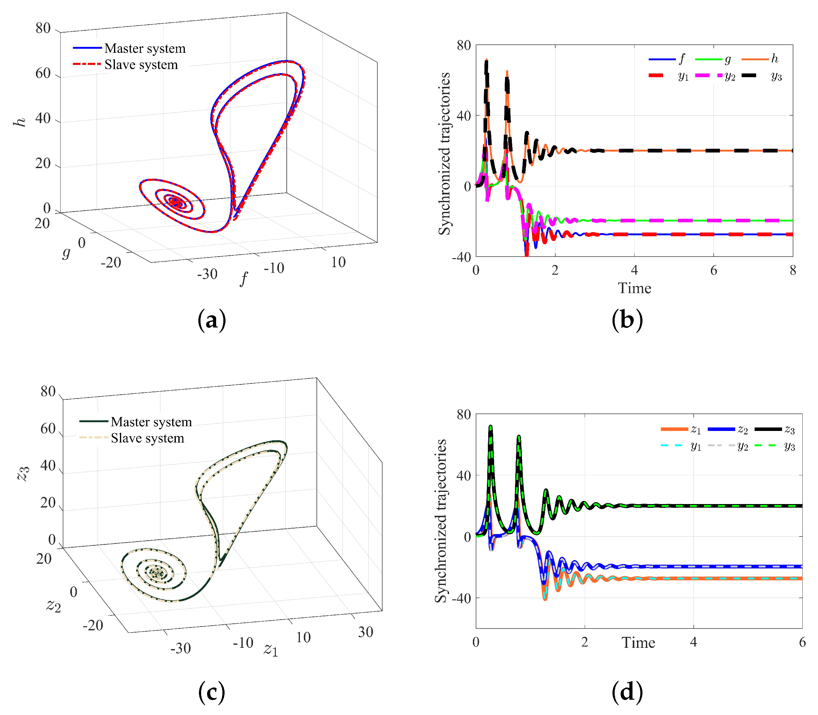
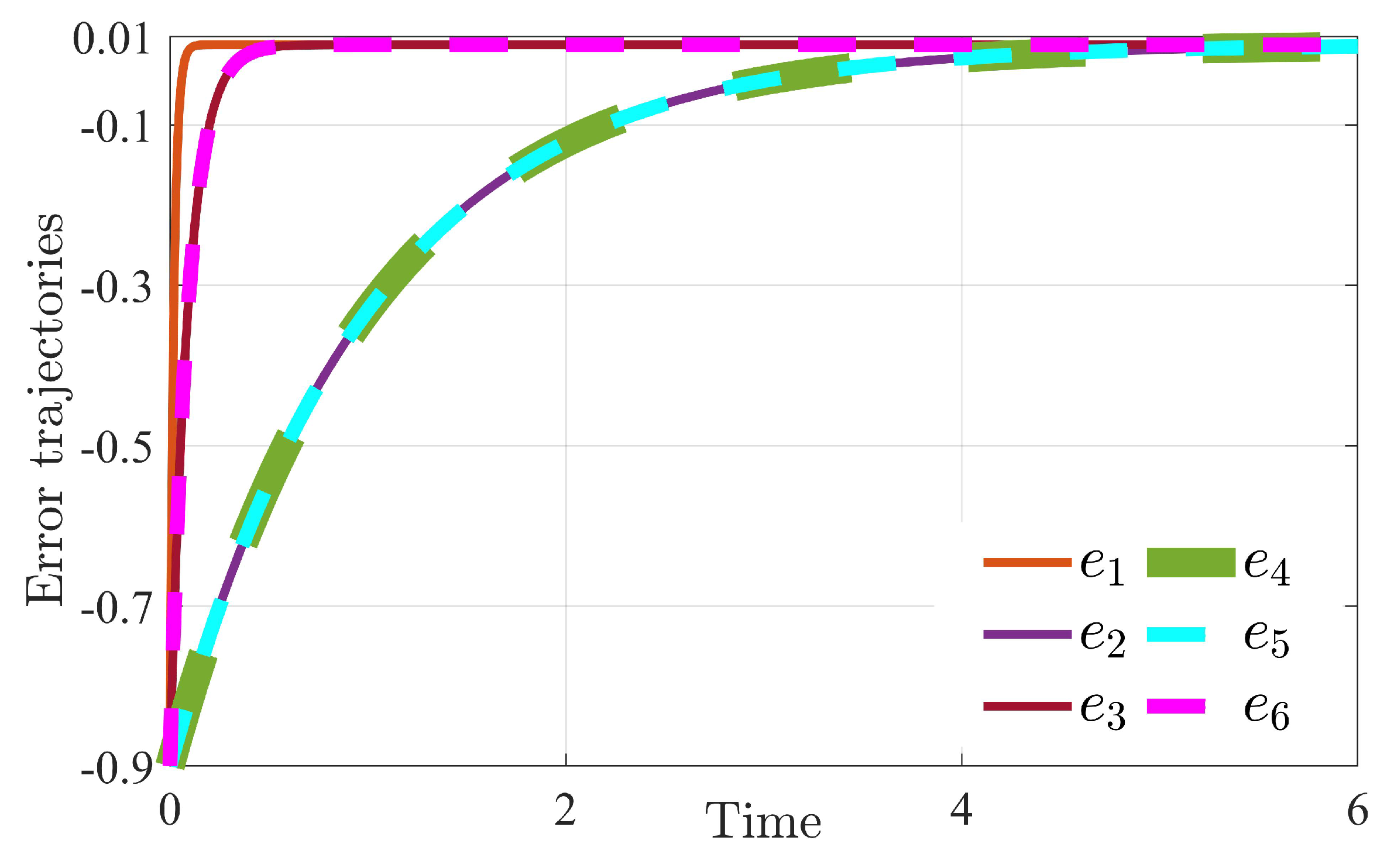
4.3. Synchronization: Discussion and Results

The synchronization techniques for chaotic systems are analyzed and illustrated in Figure 6 and Figure 7, including phase portraits, time series, and error dynamics.

Figure 6 displays the phase portraits of the synchronized chaotic system using both active and adaptive synchronization techniques. In Figure 6a, the trajectory of the slave system (shown in red) overlaps with that of the master system (shown in blue), demonstrating the synchronization achieved through the active controller. Moreover, for a more detailed analysis, their time series is plotted in Figure 6c, showing that $y_1$, $y_2$, and $y_3$ are approaching f, g, and h, respectively. Similarly, Figure 6c,d illustrate adaptive synchronization, where the slave trajectories $y_1$, $y_2$, and $y_3$ successfully overlap with the corresponding master trajectories $z_1$, $z_2$, and $z_3$, demonstrating the effectiveness of the adaptive controller. Figure 7 focuses on the error dynamics of both control techniques, where $e_1$, $e_2$, and $e_3$ are plotted using the active controller, and $e_4$, $e_4$, and $e_5$ are illustrated with the aid of the adaptive control technique. In both cases, the synchronization errors converge similarly, indicating that both methods are equally effective in reducing synchronization error terms.

The results demonstrate that both active and adaptive control techniques effectively synchronize the chaotic system, yielding identical phase portraits, state synchronizations, and synchronization errors. Remarkably, synchronization is reached by both techniques at roughly $t\approx 5$ s. This suggests that although both approaches are successful in bringing chaotic systems into synchronization, their synchronization time frames do not differ much, and both approaches are equally suitable for applications that call for chaotic system synchronization.

The findings of the current study show that adaptive and active control techniques are useful for the stabilization and synchronization of chaotic systems. Even so, due to the extremely chaotic nature of these systems, the methods used in this study could be improved by integrating robust control methods, as these systems often use disturbance and uncertainty as a primary factor. Control system resilience relies on sustaining system stability and operation within predefined parameters under unanticipated difficulties such as fracturing of system components, changes in the environment, or intrusion of hostile interference [48]. Wei et al. (2010) discussed resilient industrial control systems in their work on ‘resilient industrial control systems (RICSs)’, which proposed fundamental concepts, metrics, and perspectives for such systems [49]. Zhang et al. (2011) further advanced this work by defining resilience for manufacturing systems, particularly focusing on flexibility and recovery within volatile contexts [50]. The principles of resilience were further extended to cyber–physical systems by Zhang et al. (2010), who offered design strategies to mitigate fragility in enterprise information systems [51]. Other earlier works, including the robust stabilizers for power systems by Soliman et al. (2000) [52], the strategic power infrastructure defense (SPID) system by Liu et al. (2000) [53], and the hierarchical nonlinear switching control devised by Leonessa (2000) [54], also contributed to the development of resilient control strategies. Combining these strategies with some adaptive and active techniques could formulate a flexible hybrid paradigm, broadening the use of chaos control in practical systems.

5. Conclusions

Two control (active and adaptive) techniques were used in the current study to investigate the stability and synchronization of a novel three-dimensional chaotic system. Lyapunov theory was adopted as a tool to accomplish both tasks, while MATLAB (R2020a) simulations were plotted for the validation of their analytical results. Moreover, it was observed that at $t\approx 0.5$ s, the active control achieved desired results at both equilibrium points ($p_1$ and $p_2$), and the stabilization times for the adaptive control approach was recorded as $t\approx 0.5$ and 1 s for $p_1$ and $p_2$, respectively. These findings demonstrated that the adaptive control approach provided more flexibility in managing given system conditions, while the active control delivered faster and more consistent results.

Additionally, we synchronized two identical chaotic systems, referred to as master and slave systems, using both control strategies. MATLAB (R2020a) simulations demonstrated that both approaches successfully achieved synchronization at $t\approx 5$ s. Furthermore, these results demonstrated the effectiveness of both control techniques in bringing the 3D chaotic system into the synchronization phase. Although there were no direct applications to secure communication in our work, the findings pointed to its possibility, and it will be considered as our future target to achieve secure communication and speech recognition results.

The results pointed to the possible benefits of these kinds of systems. Active control seems beneficial for situations that require fast synchronization to create secure communication channels, whereas adaptive control dynamically adapts to various equilibrium points and changing circumstances, suggesting that secure communication may be robust, especially in complicated or noisy settings. These findings demonstrate the complementary advantages of both control strategies and point to the possibility of wider uses in the management of chaotic systems.

References

1. Zhang, T.; Xing, H.; Xu, X.; Wang, Z.; Zhao, Y. Chaos-based coverage path planning framework for mobile robots and its digital signal processing implementation. Phys. Scr. 2024, 99, 125293. [Google Scholar] [CrossRef]
2. Wang, N.; Marwan, M.; Yang, Y.; Chen, X.; Herbert, H.C.I.; Xu, Q. Designing nest-fold system via dual-route fractal process and application in chaotic mobile robot. IEEE Internet Things J. 2024, 12, 9206–9217. [Google Scholar] [CrossRef]
3. Manhil, M.M.; Jamal, R.K. A novel secure communication system using Duffing’s chaotic model. Multimed. Tools Appl. 2024, 83, 89681–89694. [Google Scholar] [CrossRef]
4. Gokyildirim, A.; Akgul, A.; Calgan, H.; Demirtas, M. Parametric fractional-order analysis of Arneodo chaotic system and microcontroller-based secure communication implementation. AEU-Int. J. Electron. Commun. 2024, 175, 155080. [Google Scholar] [CrossRef]
5. Yan, S.; Zhang, H.; Jiang, D. Multi-wing chaotic system based on smooth function and its predefined time synchronization. Commun. Nonlinear Sci. Numer. Simul. 2024, 138, 108178. [Google Scholar] [CrossRef]
6. Marwan, M.; Han, M.; Dai, Y.; Cai, M. The impact of global dynamics on the fractals of a Quadrotor Unmanned Aerial Vehicle (QUAV) chaotic system. Fractals 2024, 32, 2450043. [Google Scholar] [CrossRef]
7. Matouk, A.E. Applications of the generalized gamma function to a fractional-order biological system. Heliyon 2023, 9, e18645. [Google Scholar] [CrossRef]
8. Polyanovsky, V.O.; Kamenev, I.G. On stable and quasi-chaotic regimes in a one-dimensional unimodal mapping obtained by modeling the dynamics of a biological population. J. Phys. Conf. Ser. 2024, 2701, 012058. [Google Scholar] [CrossRef]
9. Bi, H.; Qi, G.; Hu, J. Modeling and analysis of chaos and bifurcations for the attitude system of a quadrotor unmanned aerial vehicle. Complexity 2019, 2019, 6313925. [Google Scholar] [CrossRef]
10. Ali, A.; Ahmad, J.; Javed, S.; Rehman, S. Analysis of chaotic structures, bifurcation and soliton solutions to fractional Boussinesq model. Phys. Scr. 2023, 98, 075217. [Google Scholar] [CrossRef]
11. Kocamaz, U.E.; Cevher, B.; Uyaroglu, Y. Control and synchronization of chaos with sliding mode control based on cubic reaching rule. Chaos Solitons Fractals 2017, 105, 92–98. [Google Scholar] [CrossRef]
12. Johansyah, M.D.; Sambas, A.; Mobayen, S.; Vaseghi, B.; Al-Azzawi, S.F.; Sukono; Sulaiman, I.M. Dynamical analysis and adaptive finite-time sliding mode control approach of the financial fractional-order chaotic system. Mathematics 2022, 11, 100. [Google Scholar] [CrossRef]
13. Saeed, N.A.; Saleh, H.A.; El-Ganaini, W.A.; Kamel, M.; Mohamed, M.S. On a New Three-Dimensional Chaotic System with Adaptive Control and Chaos Synchronization. Shock Vib. 2023, 2023, 1969500. [Google Scholar] [CrossRef]
14. Rahman, Z.A.; Al-Kashoash, H.A.; Ramadhan, S.M.; Al-Yasir, Y.I. Adaptive control synchronization of a novel memristive chaotic system for secure communication applications. Inventions 2019, 4, 30. [Google Scholar] [CrossRef]
15. Marwan, M.; Ahmad, S.; Aqeel, M.; Sabir, M. Control analysis of Rucklidge chaotic system. J. Dyn. Syst. Meas. Control 2019, 141, 041010. [Google Scholar] [CrossRef]
16. Yu, Z.; Zhao, F.; Ding, S.; Chen, X. Adaptive pre-assigned finite-time control of uncertain nonlinear systems with unknown control gains. Appl. Math. Comput. 2022, 417, 126784. [Google Scholar] [CrossRef]
17. Dou, W.; Ding, S.; Chen, X. Practical adaptive finite-time stabilization for a class of second-order systems. Appl. Math. Comput. 2022, 431, 127340. [Google Scholar] [CrossRef]
18. Cheng, L.; Lin, Y.; Hou, Z.; Tan, M.; Huang, J.; Zhang, W. Adaptive tracking control of hybrid machines: A closed-chain five-bar mechanism case. IEEE/ASME Trans. Mech. 2010, 16, 1155–1163. [Google Scholar] [CrossRef]
19. Barzegar, A.; Lee, D.-J. Deep reinforcement learning-based adaptive controller for trajectory tracking and altitude control of an aerial robot. Appl. Sci. 2022, 12, 4764. [Google Scholar] [CrossRef]
20. Jai, A.A.; Ouassaid, M. Three novel machine learning-based adaptive controllers for a photovoltaic shunt active power filter performance enhancement. Sci. Afr. 2024, 24, e02171. [Google Scholar]
21. He, G.; Choudhary, Y.; Shi, G. Self-Supervised Meta-Learning for All-Layer DNN-Based Adaptive Control with Stability Guarantees. arXiv 2024, arXiv:2410.07575. [Google Scholar]
22. Berkenkamp, F.; Turchetta, M.; Schoellig, A.P.; Krause, A. Safe model-based reinforcement learning with stability guarantees. Adv. Neural Inf. Process. Syst. 2017, 30, 1–11. [Google Scholar]
23. Aguilar-Lopez, R.; Martínez-Guerra, R. Chaos suppression via observer-based active control scheme: Application to Duffing’s oscillator. Chaos Solitons Fractals 2007, 32, 1887–1897. [Google Scholar] [CrossRef]
24. Roldán-Caballero, A.; Pérez-Cruz, J.H.; Hernandez-Marquez, E.; Garcia-Sanchez, J.R.; Ponce-Silva, M.; Rubio, J.D.J.; Mendoza-Chegue, A. Synchronization of a new chaotic system using adaptive control: Design and experimental implementation. Complexity 2023, 2023, 2881192. [Google Scholar] [CrossRef]
25. Kumar, A.; Handa, H. PI Sliding Mode Control and Active Control Based Stabilization Scheme for a Chaotic System Having Single Stable Equilibrium and its Circuit Implementation. In Proceedings of the 2024 5th International Conference for Emerging Technology (INCET), Belgaum, India, 24–26 May 2024; pp. 1–7. [Google Scholar]
26. Akter, M.T.; Tarammim, A.; Hussen, S. Chaos control and synchronization of modified Lorenz system using active control and backstepping scheme. Waves Random Complex Media 2023, 16, 1–20. [Google Scholar] [CrossRef]
27. Tarammim, A.; Akter, M.T. A comparative study of synchronization methods of rucklidge chaotic systems with design of active control and backstepping methods. Int. J. Mod. Nonlinear Theory Appl. 2022, 11, 31–51. [Google Scholar] [CrossRef]
28. Iqbal, S.; Wang, J. A novel fractional-order 3-D chaotic system and its application to secure communication based on chaos synchronization. Phys. Scr. 2025, 100, 025243. [Google Scholar] [CrossRef]
29. Tarammim, A.; Akter, M.T. Shimizu–Morioka’s chaos synchronization: An efficacy analysis of active control and backstepping methods. Front. Appl. Math. Stat. 2023, 9, 1100147. [Google Scholar] [CrossRef]
30. Pakiriswamy, S.; Vaidyanathan, S. Generalized projective synchronization of three-scroll chaotic systems via active control. In Proceedings of the 2012 International Conference on Computer Science and Information Technology, Bangalore, India, 2–4 January 2012; pp. 146–155. [Google Scholar]
31. Pecora, L.M.; Carroll, T.L. Synchronization in chaotic systems. Phys. Rev. Lett. 1990, 64, 821. [Google Scholar] [CrossRef]
32. Pecora, L.M.; Carroll, T.L. Driving systems with chaotic signals. Phys. Rev. A 1991, 44, 2374. [Google Scholar] [CrossRef]
33. Wang, J.; Ye, X.; Si, W. Robust ISS-satisfying fuzzy control of chaotic systems. In Proceedings of the Sixth International Conference on Intelligent Systems Design and Applications, Jinan, China, 16–18 October 2006; Volume 1, pp. 293–298. [Google Scholar]
34. Wang, X.; Liu, X.; She, K.; Zhong, S. Pinning impulsive synchronization of complex dynamical networks with various time-varying delay sizes. Nonlinear Anal. Hybrid Syst. 2017, 26, 307–318. [Google Scholar] [CrossRef]
35. Azar, A.T.; Serrano, F.; Kamal, N.A.; Koubaa, A. Robust Kinematic Control of Unmanned Aerial Vehicles with Non-holonomic Constraints. Proc. Int. Conf. Adv. Intell. Syst. Inform. 2020, 1261, 839–850. [Google Scholar]
36. Wang, L.; Dong, W.; Ding, Q. A new fixed-time sliding mode control scheme for synchronization of chaotic systems. Phys. Scr. 2024, 99, 095240. [Google Scholar] [CrossRef]
37. Marwan, M.; Mehboob, M.; Ahmad, S.; Aqeel, M. Hopf bifurcation of forced Chen system and its stability via adaptive control with arbitrary parameters. Soft Comput. 2020, 24, 4333–4341. [Google Scholar] [CrossRef]
38. Jia, T.; Chen, X.; He, L.; Zhao, F.; Qiu, J. Finite-time synchronization of uncertain fractional-order delayed memristive neural networks via adaptive sliding mode control and its application. Fractal Fract. 2022, 6, 502. [Google Scholar] [CrossRef]
39. Ogorzalek, M.J. Taming chaos. I. Synchronization. IEEE Trans. Circuits Syst. I Fundam. Theory Appl. 1993, 40, 693–699. [Google Scholar] [CrossRef]
40. Zeng, Y.; Singh, S.N. Adaptive control in Lorenz system. Int. J. Dyn. Control 1998, 8, 255–267. [Google Scholar]
41. Sambas, A.; Benkouider, K.; Kaçar, S.; Ceylan, N.; Vaidyanathan, S.; Sulaiman, I.M.; Mohamed, M.A.; Ayob, A.F.M.; Muni, S.S. Dynamic Analysis and Circuit Design of a New 3D Highly Chaotic System and its Application to Pseudo Random Number Generator (PRNG) and Image Encryption. SN Comput. Sci. 2024, 5, 420. [Google Scholar] [CrossRef]
42. Dong, Y.; Li, Y.; Li, X.; Yang, J. Active Control of Dynamic Behaviors of Graded Graphene Reinforced Cylindrical Shells with Piezoelectric Actuator/Sensor Layers. Appl. Math. Model. 2020, 82, 252–270. [Google Scholar] [CrossRef]
43. Wang, L.; Liu, J.; Yang, C.; Wu, D. A Novel Interval Dynamic Reliability Computation Approach for the Risk Evaluation of Vibration Active Control Systems Based on PID Controllers. Appl. Math. Model. 2021, 92, 422–446. [Google Scholar] [CrossRef]
44. Qin, G.; Wu, H.; Cheng, Y.; Pan, H.; Zhao, W.; Shi, S.; Song, Y.; Ji, A. Adaptive Trajectory Control of an Under-Actuated Snake Robot. Appl. Math. Model. 2022, 106, 756–769. [Google Scholar] [CrossRef]
45. Guo, X.; Wang, H.; Liu, H. Adaptive Sliding Mode Control with Disturbance Estimation for Hydraulic Actuator Systems and Application to Rock Drilling Jumbo. Appl. Math. Model. 2024, 136, 115637. [Google Scholar] [CrossRef]
46. He, Y.; Yang, M.; Zhao, X.; He, C.; Chen, Y.-H.; Li, D.; Huang, J. Adaptive Control Scheme for Cooperative Transport Systems Navigation Under Uncertainty. Appl. Math. Model. 2025, 138, 115778. [Google Scholar] [CrossRef]
47. Fiori, S. A control-theoretic approach to the synchronization of second-order continuous-time dynamical systems on real connected Riemannian manifolds. SIAM J. Control Optim. 2020, 58, 787–813. [Google Scholar] [CrossRef]
48. Rieger, C.G.; David, I.G.; McQueen, M.A. Resilient control systems: Next generation design research. In Proceedings of the 2009 2nd Conference on Human System Interactions, Catania, Italy, 21–23 May 2009. [Google Scholar]
49. Wei, D.; Ji, K. Resilient industrial control system (RICS): Concepts, formulation, metrics, and insights. In Proceedings of the 2010 3rd International Symposium on Resilient Control Systems, Idaho Falls, ID, USA, 10–12 August 2010. [Google Scholar]
50. Zhang, W.J.; Van Luttervelt, C.A. Toward a resilient manufacturing system. CIRP Ann. 2011, 60, 469–472. [Google Scholar] [CrossRef]
51. Zhang, W.; Lin, Y. On the principle of design of resilient systems–application to enterprise information systems. Enterp. Inf. Syst. 2010, 4, 99–110. [Google Scholar] [CrossRef]
52. Soliman, H.M.; Elshafei, A.L.; Shaltout, A.A.; Morsi, M.F. Robust power system stabiliser. IEE Proc.-Gener. Transm. Distrib. 2000, 147, 285–291. [Google Scholar] [CrossRef]
53. Liu, C.C.; Jung, J.; Heydt, G.T.; Vittal, V.; Phadke, A.G. The strategic power infrastructure defense (SPID) system. A conceptual design. IEEE Control Syst. Mag. 2000, 20, 40–52. [Google Scholar]
54. Leonessa, A.; Haddad, W.M.; Chellaboina, V. Hierarchical Nonlinear Switching Control Design with Applications to Propulsion Systems; Springer Science & Business Media: London, UK, 2000. [Google Scholar]
Figure 1. (a) The 3D visualization and (b) time series of system (1) showing chaos in their trajectories.
Axioms 14 00383 g001
Figure 2. Phase portraits of the (a) controlled 3 D chaotic system and (b) error dynamical system using the active controller.
Axioms 14 00383 g002
Figure 3. Time series of the state variables under active control, stabilizing at equilibrium points (a) p 1 and (b) p 2 .
Axioms 14 00383 g003
Figure 4. (a) Phase portrait and (b) time series of system (1) using adaptive control technique.
Axioms 14 00383 g004
Figure 5. (a) Error dynamics of adaptive control converging to zero, at (b) t = 1 for p 1 and (c) t = 0.5 s for p 2 .
Axioms 14 00383 g005
Figure 6. Phase portraits and time series analysis of the synchronized chaotic system using (a,b) active and (c,d) adaptive synchronization techniques.
Axioms 14 00383 g006
Figure 7. Time series of error dynamics using both control techniques.
Axioms 14 00383 g007
Disclaimer/Publisher’s Note: The statements, opinions and data contained in all publications are solely those of the individual author(s) and contributor(s) and not of MDPI and/or the editor(s). MDPI and/or the editor(s) disclaim responsibility for any injury to people or property resulting from any ideas, methods, instructions or products referred to in the content.