On Null Cartan Normal Helices in Minkowski 3-Space

Abstract

In this paper, we introduce null Cartan normal helices in Minkowski space ${\mathbb{E}}_1^3$. We obtain explicit expressions for their torsions by considering the cases when the C-constant vector field is orthogonal to their axis or not orthogonal to it. We find that the tangent vector field of a null Cartan normal helix satisfies the third-order linear homogeneous differential equation and obtain its general solution in a special case. We prove that null Cartan helices are the only normal helices having two axes and, in a particular case, three axes. Finally, we provide the necessary and sufficient conditions for null Cartan normal helices lying on a timelike surface to be isophotic curves, silhouettes, normal isophotic curves and normal silhouettes with respect to the same axis and provide some examples.

1. Introduction

In Euclidean space ${\mathbb{E}}^3$, the concept of the helix has been extended in reference [1] by means of the vector field that is constant with respect to the Frenet frame and that makes a constant angle with some fixed axis. A vector field V along a unit speed curve $\alpha$ in ${\mathbb{E}}^3$ is said to be constant with respect to a Frenet frame (or F-constant) if it satisfies the equation $V^{\prime }=D_F\times V$, where $D_F=\tau T+\kappa B$ is the Darboux vector of the Frenet frame. Every F-constant vector field has a constant length, and the sum of two F-constant vector fields is an F-constant vector field. In particular, if V is an F-constant vector field and $h\ne 0$ is some differentiable function, then $hV$ is an F-constant vector field if and only if h is a constant function. In the case when the vector field V lies in one of three characteristic planes of the curve $\alpha$, known as the normal, rectifying and osculating planes, $\alpha$ is called a normal, rectifying and osculating helix, respectively. It is proved in [1] that a unit speed curve is a normal helix with an F-constant vector field orthogonal to its axis if and only if its curvature functions $\kappa \left(s\right)>0$ and $\tau \left(s\right)\ne 0$ satisfy the equation

$${\displaystyle \frac{\kappa \left(s\right)}{{\cos }^2\theta {\kappa }^2\left(s\right)+{\tau }^2\left(s\right)}}{\left({\displaystyle \frac{\tau \left(s\right)}{\kappa \left(s\right)}}\right)}^{\prime }=-\tan \theta ,$$

for some constant $\theta \in (-\pi /2,\pi /2)$. Normal helices can be geometrically interpreted as the curves lying on a general cylinder whose normal vector field makes a constant angle with their principal normal vector. Rectifying helices whose F-constant vector field is orthogonal to their axes are general (cylindrical) helices. Osculating helices are B-directional curves of the normal helices, namely the curves whose tangent vector field is collinear with the binormal vector field of the normal helices ([1]).

Isophotic curves in Euclidean space ${\mathbb{E}}^3$ and Minkowski space ${\mathbb{E}}_1^3$ are defined by the property that the surface normal $\eta$ restricted to such curves makes a constant angle with some fixed axis W ([2,3,4]). In particular, if axis W is orthogonal to $\eta$, the curve is called a silhouette. Null Cartan isophotic curves and silhouettes lying on a timelike surface in ${\mathbb{E}}_1^3$ are generalized in [5], where it is shown that null Cartan normal isophotic curves with a non-zero constant geodesic curvature $k_g$ and geodesic torsion ${\tau }_g$ have a remarkable property in that they are general helices, relatively normal-slant helices and isophotic curves with respect to the same axis. In particular, null Cartan cubics lying on a timelike surface in ${\mathbb{E}}_1^3$ are normal isophotic curves and normal silhouettes.

In this paper, we extend the notion of normal helices in Euclidean space ${\mathbb{E}}^3$ to Minkowski space ${\mathbb{E}}_1^3$. We introduce a null Cartan normal helix with axis W as the curve, whose C-constant vector field $\tilde{N}$ lies in the normal plane of the curve and satisfies the conditions $\langle \tilde{N},W\rangle =c_0\in \mathbb{R}$ and ${\tilde{N}}^{\prime }=D_c\times \tilde{N}$, where $D_c$ is Darboux vector of the Cartan frame $\{T,N,B\}$. We consider the cases when the axis of the normal helix is orthogonal to $\tilde{N}$ and not orthogonal to it and derive the necessary and sufficient conditions for null Cartan curves to be normal helices in terms of their torsion. We prove that there are no null Cartan cubics that are normal helices with axes orthogonal to $\tilde{N}$. We conclude that null Cartan helices are the only normal helices having two axes and, in a particular case, even three. We obtain that the null tangent vector field of a null Cartan normal helix with non-constant torsion satisfies the third-order linear differential equation and find its general solution in a special case. We also show that null Cartan normal isophotic curve lying on a timelike surface with constant geodesic curvature $k_g\ne 0$, normal curvature $k_n\ne 0$ and geodesic torsion ${\tau }_g\ne 0$ is a null Cartan normal helix with respect to the same axis. Also, the null Cartan normal helix lying on a timelike cylinder with the rulings parallel to its axis is a silhouette. Finally, we give the necessary and sufficient conditions for null Cartan normal helices lying on a timelike surface in ${\mathbb{E}}_1^3$ to be silhouettes, isophotic curves, normal silhouettes and normal isophotic curves in terms of their geodesic curvature and provide some examples.

By using similar methods, other types of helices can be defined in Minkowski space ${\mathbb{E}}_1^3$, including null Cartan rectifying helices, null Cartan osculating helices and their spacelike and timelike counterparts. Finally, the results presented in this paper can be extended to other ambient spaces such as Galilean space ${\mathbb{G}}_3$, pseudo-Galilean space ${\mathbb{G}}_3^1$ and dual space ${\mathbb{D}}^3$.

2. Preliminaries

A three-dimensional Minkowski space ${\mathbb{E}}_1^3$ is a real vector space ${\mathbb{R}}^3$ endowed with an indefinite scalar product given by

$$〈x,y〉=-x_1{y}_1+x_2{y}_2+x_3{y}_3,$$

for any two vectors $x=(x_1,x_2,x_3)$ and $y=(y_1,y_2,y_3)$. An arbitrary vector $v\ne 0$ in ${\mathbb{E}}_1^3$ is said to be spacelike, timelike or null (lightlike) if it satisfies $〈v,v〉>0$, $〈v,v〉<0$ or $〈v,v〉=0$, respectively [6]. A vector $v=0$ is said to be spacelike. The norm (length) of a vector v is given by $∥v∥=\sqrt{\left|〈v,v〉\right|}$.

The vector product of two vectors $x=(x_1,x_2,x_3)$ and $y=(y_1,y_2,y_3)$ in ${\mathbb{E}}_1^3$ is defined by

$$x\times y=(x_3{y}_2-x_2{y}_3,x_3{y}_1-x_1{y}_3,x_1{y}_2-x_2{y}_1).$$

An arbitrary curve $\gamma :I\to {\mathbb{E}}_1^3$ is said to be spacelike, timelike or null (lightlike) if all of its velocity vectors ${\gamma }^{\prime }$ are spacelike, timelike or null, respectively [6].

A null curve $\alpha :I\to E_1^3$ parameterized by pseudo-arc function

$$s\left(t\right)={\int }_0^t\Vert {\alpha }^{″}\left(u\right){\Vert }^{{\displaystyle \frac{1}{2}}}du,$$

where ${\alpha }^{″}\left(t\right)\ne 0$ for all $t\in I$ is called a null Cartan curve ([7]). There exists a positively oriented Cartan frame $\{T,N,B\}$ of $\alpha$ that satisfies the conditions

$$〈T,T〉=〈B,B〉=\langle T,N\rangle =〈N,B〉=0,〈N,N〉=1,〈T,B〉=ϵ=\pm 1,$$

(1)

$$T\times N=ϵT,N\times B=ϵB,B\times T=N,$$

(2)

$$det(T,N,B)=[T,N,B]=1.$$

(3)

The Cartan frame’s equations read [8,9]

$$\left[\begin{array}{c}{T}^{\prime }\\ N^{\prime }\\ B^{\prime }\end{array}\right]=\left[\begin{array}{ccc}0& \kappa & 0\\ ϵ\tau & 0& -ϵ\kappa \\ 0& -\tau & 0\end{array}\right]\left[\begin{array}{c}T\\ N\\ B\end{array}\right],$$

(4)

where $\kappa \left(s\right)=1$ for each s is the curvature and $\tau \left(s\right)$ is the torsion of $\alpha$. If $\tau \left(s\right)=0$ for each s, $\alpha$ is called a null Cartan cubic. If $\tau \left(s\right)=constant\ne 0$ for each s, $\alpha$ is called a null Cartan helix.

The Darboux vector (centrode, angular velocity vector) of Cartan frame has the parameter equation

$$D_c\left(s\right)=\tau \left(s\right)T\left(s\right)+B\left(s\right)$$

and satisfies Darboux equations

$$T^{\prime }=D_c\times T,N^{\prime }=D_c\times N,B^{\prime }=D_c\times B.$$

(5)

A surface M in ${\mathbb{E}}_1^3$ is timelike if the induced metric in all of its tangent planes is a non-degenerate of index one. A timelike ruled surface $x(s,t)=\alpha \left(s\right)+tB\left(s\right)$ with a null Cartan base curve $\alpha$ and rulings parallel to the binormal vector field B is called B-scroll.

The Darboux frame $\{T,\zeta ,\eta \}$ of a null Cartan curve $\alpha$ lying on a timelike surface contains the tangential vector field T, the unit spacelike normal vector field

$$\eta ={\displaystyle \frac{x_u\times x_t}{\left|\right|x_u\times x_t\left|\right|}}{|}_{\alpha }$$

and the null transversal vector field $\zeta$. Such vector fields satisfy the conditions [5]

$$\langle T,T\rangle =\langle \zeta ,\zeta \rangle =\langle T,\eta \rangle =\langle \zeta ,\eta \rangle =0,\langle \eta ,\eta \rangle =1,\langle T,\zeta \rangle ={ϵ}_1=\pm 1,$$

(6)

$$T\times \zeta =\eta ,\zeta \times \eta ={ϵ}_1\zeta ,\eta \times T={ϵ}_{1}T,det(T,\zeta ,\eta )=[T,\zeta ,\eta ]=1.$$

(7)

In particular, Darboux frame’s equations have the form [5]

$$\left[\begin{array}{c}{T}^{\prime }\\ {\zeta }^{\prime }\\ {\eta }^{\prime }\end{array}\right]=\left[\begin{array}{ccc}{ϵ}_1{k}_g& 0& k_n\\ 0& -{ϵ}_1{k}_g& {\tau }_g\\ -{ϵ}_1{\tau }_g& -{ϵ}_1{k}_n& 0\end{array}\right]\left[\begin{array}{c}T\\ \zeta \\ \eta \end{array}\right],$$

(8)

where $k_g=\langle T^{\prime },\zeta \rangle$, $k_n=\langle T^{\prime },\eta \rangle =-ϵ{ϵ}_1$ and ${\tau }_g=\langle {\zeta }^{\prime },\eta \rangle$ are the geodesic curvature, normal curvature and geodesic torsion of $\alpha$, respectively.

The relation between the Cartan and Darboux frame of $\alpha$ reads ([5])

$$\left[\begin{array}{c}T\\ N\\ B\end{array}\right]=\left[\begin{array}{ccc}1& 0& 0\\ {ϵ}_1{k}_g& 0& k_n\\ {\displaystyle -\frac{ϵ}{2}{k}_g^2}& -k_n& k_g\end{array}\right]\left[\begin{array}{c}T\\ \zeta \\ \eta \end{array}\right],$$

(9)

The generalized Darboux frame of the first kind of $\alpha$ is given by [5]

$$\left[\begin{array}{c}\tilde{T}\\ \tilde{\zeta }\\ \tilde{\eta }\end{array}\right]=\left[\begin{array}{ccc}\mu & 0& 0\\ -{ϵ}_1{\displaystyle \frac{{\lambda }^2}{2\mu }}& {\displaystyle \frac{1}{\mu }}& -{ϵ}_1{\displaystyle \frac{\lambda }{\mu }}\\ \lambda & 0& 1\end{array}\right]\left[\begin{array}{c}T\\ \zeta \\ \eta \end{array}\right],$$

(10)

where $\lambda \left(s\right)\ne 0$ and $\mu \left(s\right)\ne 0$ are some differentiable functions satisfying the Bernoulli differential equation

$$2{ϵ}_1{\lambda }^{\prime }\left(s\right)+2\lambda \left(s\right)k_g\left(s\right)-{ϵ}_1{\lambda }^2\left(s\right)k_n\left(s\right)=0,$$

(11)

and the first-order linear differential equation

$${\mu }^{\prime }\left(s\right)-\mu \left(s\right)\lambda \left(s\right)k_n\left(s\right)=0.$$

Throughout the next sections, let ${\mathbb{R}}_0$ denote $\mathbb{R}\backslash \left\{0\right\}$.

3. Null Cartan Normal Helices in ${\mathbf{𝔼}}_{\mathbf{1}}^{\mathbf{3}}$

In this section, we introduce the null Cartan normal helix in ${\mathbb{E}}_1^3$ with an axis of W by means of the vector field $\tilde{N}$ that is constant with respect to the Cartan frame $\{T,N,B\}$, lies in the normal plane $T^{\perp }=span\{T,N\}$ and satisfies the condition $\langle \tilde{N},W\rangle =constant$. By considering the cases when axis W is orthogonal to $\tilde{N}$ and not orthogonal to it, we provide the necessary and sufficient conditions for the null Cartan curve to be a normal helix. We obtain the third-order linear differential equation for the tangent vector field of the null Cartan normal helix with non-constant torsion, whose general solution provides its parameter equation. We firstly define the vector field that is constant with respect to the Cartan frame.

Definition 1. 

The vector field V of a null Cartan curve with Cartan frame $\{T,N,B\}$ in ${\mathbb{E}}_1^3$ is said to be constant with respect to the Cartan frame (or C-constant) if it satisfies the equation

$$V^{\prime }\left(s\right)=D_c\left(s\right)\times V\left(s\right),$$

where $D_c\left(s\right)=\tau \left(s\right)T\left(s\right)+B\left(s\right)$ is the Darboux vector of the Cartan frame.

According to (5), the vector fields of the Cartan frame are C-constant vector fields. In general case, an arbitrary C-constant vector field is a linear combination of the Cartan frame’s vector fields. It can be easily checked that a C-constant vector field has a constant length and that a sum of two C-constant vector fields is a C-constant vector field. In particular, if V is a C-constant vector field and $h\ne 0$ is some differentiable function, then $hV$ is a C-constant vector field if and only if h is a constant function.

Definition 2. 

A null Cartan curve with a Cartan frame $\{T,N,B\}$ in ${\mathbb{E}}_1^3$ is called a normal helix if there exists a unit C-constant vector field $\tilde{N}={\lambda }_{0}T+N$ of α and a fixed axis $W\in {\mathbb{E}}_1^3$, satisfying the condition

$$\langle \tilde{N},W\rangle =c_0,$$

(12)

where ${\lambda }_0\in {\mathbb{R}}_0$ and $c_0\in \mathbb{R}$.

The vector field $\tilde{N}$ lies in the normal plane $T^{\perp }=span\{T,N\}$ of the null Cartan curve $\alpha$. It can be easily verified that it is C-constant, as Darboux Equation (5) implies

$${\tilde{N}}^{\prime }={\lambda }_0{T}^{\prime }+N^{\prime }={\lambda }_0{D}_c\times T+D_c\times N=D_c\times \tilde{N}.$$

In particular, ${\tilde{N}}^{\prime }=ϵ\tau T+{\lambda }_{0}N-ϵB\ne 0$, so $\tilde{N}$ is not a constant vector field. Assume that an axis W of a null Cartan normal helix has a parameter equation of the form

$$W\left(s\right)=a\left(s\right)T\left(s\right)+b\left(s\right)N\left(s\right)+c\left(s\right)B\left(s\right),$$

(13)

where $a\left(s\right)$, $b\left(s\right)$ and $c\left(s\right)$ are some differentiable functions in pseudo-arc s. By using (4), (12) and the condition $W^{\prime }\left(s\right)=0$, we obtain the system of equations

$$\begin{array}{ccc}\hfill a^{\prime }\left(s\right)+ϵ\tau \left(s\right)b\left(s\right)& =& 0,\hfill \end{array}$$

(14)

$$\begin{array}{ccc}\hfill a\left(s\right)+b^{\prime }\left(s\right)-c\left(s\right)\tau \left(s\right)& =& 0,\hfill \end{array}$$

(15)

$$\begin{array}{ccc}\hfill c^{\prime }\left(s\right)-ϵb\left(s\right)& =& 0,\hfill \end{array}$$

(16)

$$\begin{array}{ccc}\hfill b\left(s\right)+ϵ{\lambda }_{0}c\left(s\right)-c_0& =& 0,\hfill \end{array}$$

(17)

whose solution provides the necessary and sufficient conditions for a null Cartan curve to be a normal helix. In the theorems that follow, we will consider the cases when an axis of a null Cartan normal helix is orthogonal to C-constant vector field ($c_0=0$) or not orthogonal to it ($c_0\ne 0$).

Theorem 1. 

A null Cartan curve α with the torsion $\tau \left(s\right)\ne constant$ in ${\mathbb{E}}_1^3$ is a normal helix with axis W satisfying $\langle \tilde{N},W\rangle =c_0\ne 0$ if and only if its torsion is given by

$$\tau \left(s\right)={\displaystyle \frac{c_1}{c^2\left(s\right)}}+ϵ{\displaystyle \frac{{\lambda }_0^2}{2}},$$

(18)

where $c\left(s\right)={\displaystyle \frac{ϵ}{{\lambda }_0}}(c_0-\tilde{c}{e}^{-{\lambda }_{0}s})$, $\tilde{c}\in {\mathbb{R}}^{+}$, $c_1,c_0,{\lambda }_0\in {\mathbb{R}}_0$.

Proof. 

Assume that $\alpha$ is a normal helix with axis W given by (13) and satisfying $\langle \tilde{N},W\rangle =c_0\ne 0$. By using (15)–(17), we obtain

$$a\left(s\right)=c\left(s\right)\tau \left(s\right)-b^{\prime }\left(s\right)=c\left(s\right)\tau \left(s\right)-{(c_0-ϵ{\lambda }_{0}c\left(s\right))}^{\prime }=c\left(s\right)\tau \left(s\right)+{\lambda }_{0}b\left(s\right).$$

Substituting this in (14) and using (16), we find

$${(c\left(s\right)\tau \left(s\right)+{\lambda }_{0}b\left(s\right))}^{\prime }+\tau \left(s\right)c^{\prime }\left(s\right)=0.$$

From (17), we obtain $b^{\prime }\left(s\right)=-ϵ{\lambda }_0{c}^{\prime }\left(s\right)$. Hence, the previous differential equation reads

$${\tau }^{\prime }\left(s\right)+2{\displaystyle \frac{c^{\prime }\left(s\right)}{c\left(s\right)}}\tau \left(s\right)=ϵ{\lambda }_0^2{\displaystyle \frac{c^{\prime }\left(s\right)}{c\left(s\right)}}.$$

Its general solution has the form

$$\tau \left(s\right)={\displaystyle \frac{c_1}{c^2\left(s\right)}}+ϵ{\displaystyle \frac{{\lambda }_0^2}{2}},$$

where $c_1\in {\mathbb{R}}_0$. Differentiating (17) with respect to s and using (16), we find $b^{\prime }\left(s\right)=-{\lambda }_{0}b\left(s\right)$ and thus $b\left(s\right)=\tilde{c}{e}^{-{\lambda }_{0}s}$, $\tilde{c}\in {\mathbb{R}}^{+}$. In particular, from (17), we obtain $c\left(s\right)={\displaystyle \frac{ϵ}{{\lambda }_0}}(c_0-b\left(s\right))$. Consequently, relation (18) holds.

Conversely, assume that the torsion of the null Cartan curve $\alpha$ is given by (18). Let us consider an axis W with parameter Equation (13). Then, $W^{\prime }\left(s\right)=0$ if and only if the system of Equations (14)–(16) holds. By using (16), we obtain $b\left(s\right)=ϵc^{\prime }\left(s\right)=\tilde{c}{e}^{-{\lambda }_{0}s}$. From (15) and (18), we find $a\left(s\right)={\displaystyle \frac{c_1}{c\left(s\right)}}+{\displaystyle \frac{{\lambda }_0}{2}}(b\left(s\right)+c_0)$. Hence, the solution of the system of Equations (14)–(16) reads

$$a\left(s\right)={\displaystyle \frac{c_1}{c\left(s\right)}}+{\displaystyle \frac{{\lambda }_0}{2}}(b\left(s\right)+c_0),b\left(s\right)=\tilde{c}{e}^{-{\lambda }_{0}s},c\left(s\right)={\displaystyle \frac{ϵ}{{\lambda }_0}}(c_0-b\left(s\right)).$$

Substituting this in (13), we obtain that the axis has the parameter equation

$$W\left(s\right)=({\displaystyle \frac{c_1}{c\left(s\right)}}+{\displaystyle \frac{{\lambda }_0}{2}}(b\left(s\right)+c_0))T\left(s\right)+b\left(s\right)N\left(s\right)+{\displaystyle \frac{ϵ}{{\lambda }_0}}(c_0-b\left(s\right))B\left(s\right).$$

(19)

Relations (1) and (19) yield $\langle \tilde{N}\left(s\right),W\left(s\right)\rangle =c_0$. Because there exists an axis satisfying $\langle \tilde{N}\left(s\right),W\left(s\right)\rangle =c_0\ne 0$, $\alpha$ is a normal helix with axis W. □

By using (4) and (18), the next theorem can be easily proved.

Theorem 2. 

The tangent vector field of the null Cartan normal helix with a torsion given by (18) satisfies the third-order linear differential equation

$$c^3\left(s\right)T^{‴}\left(s\right)-c\left(s\right)(2ϵc_1+c^2\left(s\right){\lambda }_0^2)T^{\prime }\left(s\right)+2ϵc_1{c}^{\prime }\left(s\right)T\left(s\right)=0,$$

(20)

where $c\left(s\right)={\displaystyle \frac{ϵ}{{\lambda }_0}}(c_0-\tilde{c}{e}^{-{\lambda }_{0}s})$, $\tilde{c}\in {\mathbb{R}}^{+}$, $c_1,c_0,{\lambda }_0\in {\mathbb{R}}_0$.

Differential Equation (20) cannot be explicitly solved in a general case. However, it is possible in some cases.

Example 1. 

Assume that the tangent vector field of null Cartan normal helix α satisfies (20). By choosing arbitrary constants ${\lambda }_0=c_0=-1$ and $\tilde{c}=ϵ=c_1=1$, we obtain $c\left(s\right)=e^s+1$. Hence, differential Equation (20) reads

$${(e^s+1)}^3{T}^{‴}\left(s\right)-2(e^s+1)T^{\prime }\left(s\right)-{(e^s+1)}^3{T}^{\prime }\left(s\right)+2e^{s}T\left(s\right)=0.$$

Its general solution is given by

$$T\left(s\right)=C_1(e^s+1)+C_2{\displaystyle \frac{(e^s+1){\left(\frac{e^s}{e^s+1}\right)}^{\sqrt{3}}}{\sqrt{3}}}+C_3(e^s+1){\left({\displaystyle \frac{e^s}{e^s+1}}\right)}^{-\sqrt{3}},$$

where $C_1,C_2,C_3$ are constant vectors in ${\mathbb{E}}_1^3$. Up to isometries of ${\mathbb{E}}_1^3$, we may choose $C_1=(0,0,{\displaystyle \frac{1}{\sqrt{3}}})$, $C_2=(\sqrt{3},\sqrt{3},0)$ and $C_3=({\displaystyle \frac{1}{4}},-{\displaystyle \frac{1}{4}},0)$. Consequently, the parameter equation of the tangent vector field has the form

$$T\left(s\right)={\displaystyle \frac{e^s+1}{\sqrt{3}}}\left({\left({\displaystyle \frac{e^s}{e^s+1}}\right)}^{\sqrt{3}}+{\displaystyle \frac{1}{4}}{\left({\displaystyle \frac{e^s}{e^s+1}}\right)}^{-\sqrt{3}},{\left({\displaystyle \frac{e^s}{e^s+1}}\right)}^{\sqrt{3}}-{\displaystyle \frac{1}{4}}{\left({\displaystyle \frac{e^s}{e^s+1}}\right)}^{-\sqrt{3}},1\right).$$

(21)

It can be easily verified that (21) yields $\langle T\left(s\right),T\left(s\right)\rangle =0$ and $\langle T^{\prime }\left(s\right),T^{\prime }\left(s\right)\rangle =1$. By integrating (21), we find the parameter equation of the null Cartan normal helix as

$$\begin{array}{ccc}\hfill \alpha \left(s\right)& =& {\displaystyle \frac{1}{\sqrt{3}}}(\int (e^s+1)\left({\left({\displaystyle \frac{e^s}{e^s+1}}\right)}^{\sqrt{3}}+{\displaystyle \frac{1}{4}}{\left({\displaystyle \frac{e^s}{e^s+1}}\right)}^{-\sqrt{3}}\right)ds,\hfill \\ & & \int (e^s+1)\left({\left({\displaystyle \frac{e^s}{e^s+1}}\right)}^{\sqrt{3}}-{\displaystyle \frac{1}{4}}{\left({\displaystyle \frac{e^s}{e^s+1}}\right)}^{-\sqrt{3}}\right)ds,e^s+s).\hfill \end{array}$$

Theorem 3. 

Every null Cartan helix in ${\mathbb{E}}_1^3$ with torsion $\tau \left(s\right)={\tau }_0\in {\mathbb{R}}_0$ is a normal helix with axis

$$W\left(s\right)={\displaystyle \frac{ϵc_0{\tau }_0}{{\lambda }_0}}T\left(s\right)+{\displaystyle \frac{ϵc_0}{{\lambda }_0}}B\left(s\right),$$

(22)

satisfying $\langle \tilde{N},W\rangle =c_0\ne 0$ and if ${\tau }_0={\displaystyle \frac{ϵ{\lambda }_0^2}{2}}$ with an additional axis

$$W\left(s\right)={\displaystyle \frac{{\lambda }_0}{2}}(b\left(s\right)+c_0)T\left(s\right)+b\left(s\right)N\left(s\right)+{\displaystyle \frac{ϵ}{{\lambda }_0}}(c_0-b\left(s\right))B\left(s\right),$$

(23)

satisfying $\langle \tilde{N},W\rangle =c_0\ne 0$, where $b\left(s\right)=\tilde{c}{e}^{-{\lambda }_{0}s}$, $\tilde{c}\in {\mathbb{R}}^{+}$.

Proof. 

Assume that $\alpha$ is a null Cartan helix with torsion $\tau \left(s\right)={\tau }_0\in {\mathbb{R}}_0$ and an axis W given by (13). Then, $W^{\prime }\left(s\right)=0$ if and only if the system of Equations (14)–(16) hold. By solving the mentioned system of equations and using $\tau \left(s\right)={\tau }_0$, we obtain the differential equation

$$b^{″}\left(s\right)=2ϵ{\tau }_{0}b\left(s\right).$$

(24)

We may consider two possibilities: ($1^{\circ }$) $b\left(s\right)=0$. Relations (15) and (16) give $c\left(s\right)=constant\ne 0$, $a\left(s\right)={\tau }_{0}c\left(s\right)$. Then, W satisfies $\langle \tilde{N},W\rangle =c_0\ne 0$ if and only if $c\left(s\right)={\displaystyle \frac{ϵc_0}{{\lambda }_0}}$. Substituting $a\left(s\right)$, $b\left(s\right)$ and $c\left(s\right)$ in (13), we find that W has parameter Equation (22). ($2^{\circ }$) $b\left(s\right)\ne 0$. Differential Equation (24) has the general solution

$$b\left(s\right)=c_1{e}^{\sqrt{2ϵ{\tau }_0}s}+c_2{e}^{-\sqrt{2ϵ{\tau }_0}s},$$

(25)

where $2ϵ{\tau }_0>0$, $c_1,c_1\in \mathbb{R}$. Then, W satisfies $\langle \tilde{N},W\rangle =c_0\ne 0$ if and only if (17) holds. Differentiating (17) with respect to s and using (16), we find $b\left(s\right)=\tilde{c}{e}^{-{\lambda }_{0}s}$, $\tilde{c}\in {\mathbb{R}}^{+}$. The last relation together with (25) gives $c_1=0$, $c_2=\tilde{c}$, ${\tau }_0={\displaystyle \frac{ϵ{\lambda }_0^2}{2}}$. From (17), we find $c\left(s\right)={\displaystyle \frac{ϵ}{{\lambda }_0}}(c_0-b\left(s\right))$. Hence, relations (15)–(17) and ${\tau }_0={\displaystyle \frac{ϵ{\lambda }_0^2}{2}}$ imply $a\left(s\right)={\displaystyle \frac{{\lambda }_0}{2}}(c_0+b\left(s\right))$. Consequently, W has parameter Equation (23).

Because in both cases ($1^{\circ }$) and ($2^{\circ }$), there exists a fixed axis satisfying $\langle \tilde{N},W\rangle =c_0\in {\mathbb{R}}_0$, the curve $\alpha$ is a normal helix with an axis W. □

Example 2. 

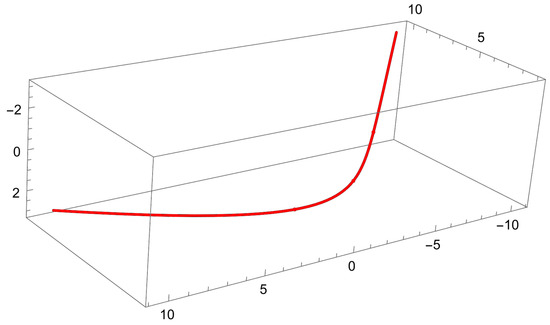
Let α be the null Cartan normal helix with the torsion $\tau \left(s\right)=ϵ{\displaystyle \frac{{\lambda }_0^2}{2}}$, ${\lambda }_0\in {\mathbb{R}}_0$, $ϵ=\pm 1$. By using (4) and $\tau \left(s\right)=ϵ{\displaystyle \frac{{\lambda }_0^2}{2}}$, we obtain the differential equation

$$T^{‴}\left(s\right)-{\lambda }_0^2{T}^{\prime }\left(s\right)=0.$$

Its general solution reads

$$T\left(s\right)={\displaystyle \frac{1}{{\lambda }_0}}(\cosh \left({\lambda }_{0}s\right),\sinh \left({\lambda }_{0}s\right),1)$$

and therefore, the parameter equation of α has the form (Figure 1)

$$\alpha \left(s\right)=\int T\left(s\right)ds={\displaystyle \frac{1}{{\lambda }_0}}({\displaystyle \frac{1}{{\lambda }_0}}\sinh \left({\lambda }_{0}s\right),{\displaystyle \frac{1}{{\lambda }_0}}\cosh \left({\lambda }_{0}s\right),s).$$

From (1) and (4), we find

$$N\left(s\right)=(\sinh \left({\lambda }_{0}s\right),\cosh \left({\lambda }_{0}s\right),0),B\left(s\right)={\displaystyle \frac{ϵ{\lambda }_0}{2}}(-\cosh \left({\lambda }_{0}s\right),-\sinh \left({\lambda }_{0}s\right),1).$$

Putting ${\lambda }_0=1$, relations (22) and (23) imply that α has the axes

$$W\left(s\right)={\displaystyle \frac{c_0}{2}}T\left(s\right)+ϵc_{0}B\left(s\right)=(0,0,c_0),$$

and

$$W_1\left(s\right)={\displaystyle \frac{1}{2}}(b\left(s\right)+c_0)T\left(s\right)+b\left(s\right)N\left(s\right)+ϵ(c_0-b\left(s\right))B\left(s\right)=(\tilde{c},\tilde{c},c_0),$$

where $b\left(s\right)=\tilde{c}{e}^{-s}$, $\tilde{c}\in {\mathbb{R}}^{+}$, satisfying $\langle \tilde{N}\left(s\right),W\left(s\right)\rangle =\langle \tilde{N}\left(s\right),W_1\left(s\right)\rangle =c_0$.

Theorem 4. 

Every null Cartan cubic in ${\mathbb{E}}_1^3$ is a normal helix with axis

$$W\left(s\right)=ϵ{\displaystyle \frac{c_0}{{\lambda }_0}}B\left(s\right)$$

(26)

satisfying $\langle \tilde{N},W\rangle =c_0\ne 0$, $ϵ=\pm 1$, ${\lambda }_0\in {\mathbb{R}}_0$.

Proof. 

Suppose that $\alpha$ is a null Cartan cubic with an axis $W\left(s\right)$ given by (13). Then, $W\left(s\right)$ is a fixed axis if and only if the system of Equations (14)–(16) hold. By solving the mentioned system of equations, we obtain

$$a\left(s\right)=b\left(s\right)=0,c\left(s\right)=constant\ne 0.$$

Then, W satisfies the condition $\langle \tilde{N},W\rangle =c_0\ne 0$ if and only if $c\left(s\right)={\displaystyle \frac{ϵc_0}{{\lambda }_0}}$. Substituting $a\left(s\right)$, $b\left(s\right)$ and $c\left(s\right)$ in (13), we find that W has parameter Equation (26). Hence, $\alpha$ is a normal helix with a lightlike axis W. □

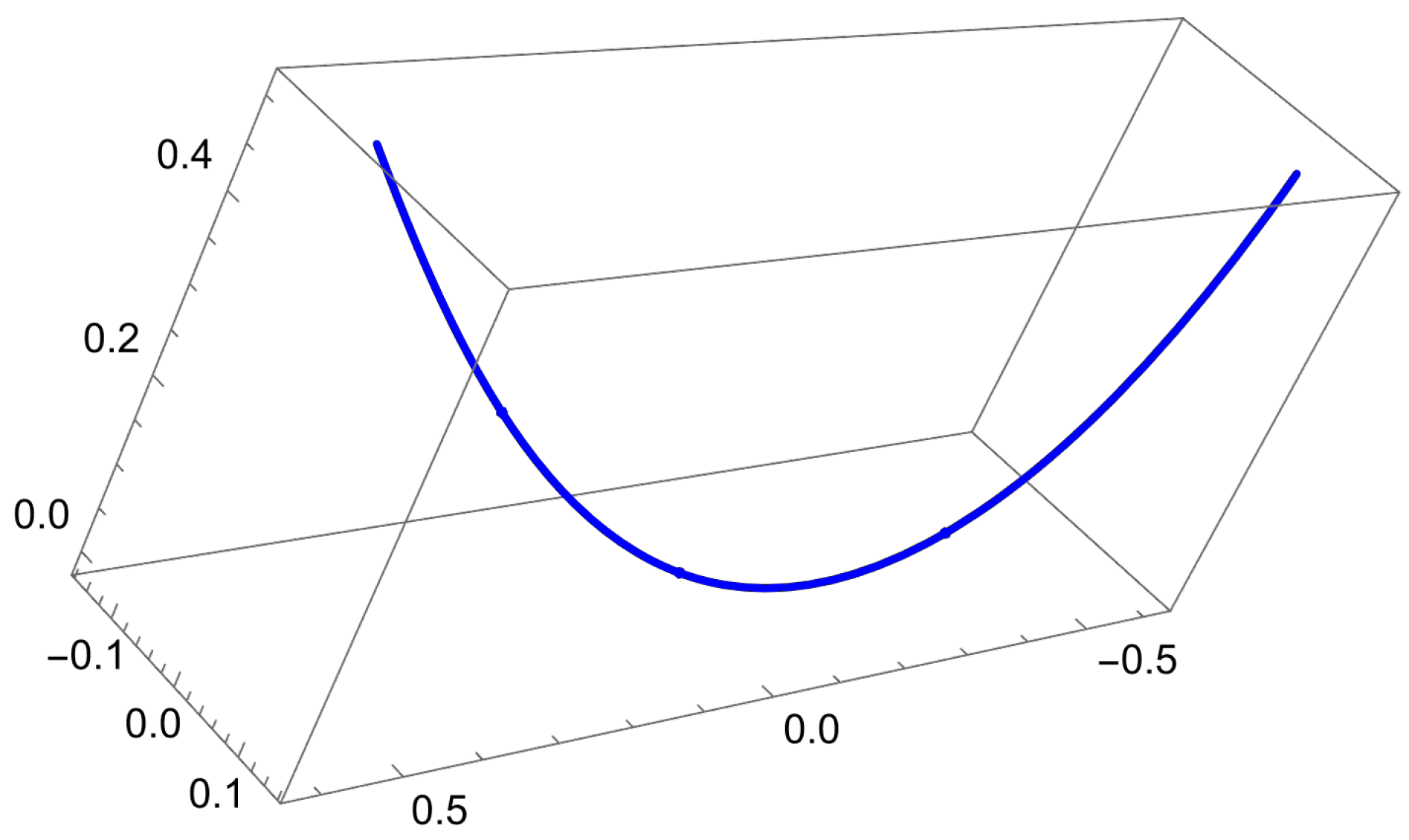
According to Theorem 3 and relation (26), the null Cartan cubic with parameter equation

$$\alpha \left(s\right)=({\displaystyle \frac{s^3}{4}}+{\displaystyle \frac{s}{3}},{\displaystyle \frac{s^3}{4}}-{\displaystyle \frac{s}{3}},{\displaystyle \frac{s^2}{2}})$$

and Cartan frame

$$T\left(s\right)=({\displaystyle \frac{3s^2}{4}}+{\displaystyle \frac{1}{3}},{\displaystyle \frac{3s^2}{4}}-{\displaystyle \frac{1}{3}},s),N\left(s\right)=({\displaystyle \frac{3s}{2}},{\displaystyle \frac{3s}{2}},1),B\left(s\right)=(-{\displaystyle \frac{3}{2}},-{\displaystyle \frac{3}{2}},0),$$

is a normal helix with a lightlike axis given by (Figure 2)

$$W\left(s\right)=ϵ{\displaystyle \frac{c_0}{{\lambda }_0}}B\left(s\right)={\displaystyle \frac{c_0}{{\lambda }_0}}(-{\displaystyle \frac{3}{2}},-{\displaystyle \frac{3}{2}},0).$$

Moreover, relation (26) implies $\langle T,W\rangle ={\displaystyle \frac{c_0}{{\lambda }_0}}$, $\langle N,W\rangle =0$. Therefore, the next statement holds.

Corollary 1. 

Every null Cartan cubic in ${\mathbb{E}}_1^3$ is a normal helix, general helix and slant helix with respect to the same axis that is not orthogonal to C-constant vector field $\tilde{N}$.

In the case when an axis of the null Cartan normal helix is orthogonal to C-constant vector field $\tilde{N}$, we obtain the next theorems.

Theorem 5. 

A null Cartan curve α with the torsion $\tau \left(s\right)\ne constant$ in ${\mathbb{E}}_1^3$ is a normal helix with axis W satisfying $\langle \tilde{N},W\rangle =0$ if and only if its torsion is given by

$$\tau \left(s\right)={\displaystyle \frac{c_2}{c^2\left(s\right)}}+ϵ{\displaystyle \frac{{\lambda }_0^2}{2}},$$

(27)

where $c\left(s\right)=-{\displaystyle \frac{ϵ}{{\lambda }_0}}\tilde{c}{e}^{-{\lambda }_{0}s}$, $\tilde{c}\in {\mathbb{R}}^{+}$, $c_2,{\lambda }_0\in {\mathbb{R}}_0$.

Proof. 

Suppose that an axis W of $\alpha$ given by (13) satisfies the condition $\langle \tilde{N},W\rangle =0$. By using the condition $W^{\prime }\left(s\right)=0$, we obtain that the torsion of $\alpha$ is given by (27), where $c\left(s\right)=-{\displaystyle \frac{ϵ}{{\lambda }_0}}\tilde{c}{e}^{-{\lambda }_{0}s}$, $\tilde{c}\in {\mathbb{R}}^{+}$, $c_2{\lambda }_0\in {\mathbb{R}}_0$.

Conversely, assume that the torsion of the null Cartan curve $\alpha$ is given by (27). Let us consider axis W with parameter Equation (13). Then, $W^{\prime }\left(s\right)=0$ if and only if the system of Equations (14)–(16) holds. By using (16) and $c\left(s\right)=-{\displaystyle \frac{ϵ}{{\lambda }_0}}\tilde{c}{e}^{-{\lambda }_{0}s}$, we find $b\left(s\right)=ϵc^{\prime }\left(s\right)=\tilde{c}{e}^{-{\lambda }_{0}s}$. From (15) and (27), we obtain $a\left(s\right)={\displaystyle \frac{c_2}{c\left(s\right)}}+{\displaystyle \frac{{\lambda }_0}{2}}b\left(s\right)$. Consequently, the solution of the system of Equations (14)–(16) reads

$$a\left(s\right)={\displaystyle \frac{c_2}{c\left(s\right)}}+{\displaystyle \frac{{\lambda }_0}{2}}b\left(s\right),b\left(s\right)=\tilde{c}{e}^{-{\lambda }_{0}s},c\left(s\right)=-{\displaystyle \frac{ϵ}{{\lambda }_0}}b\left(s\right).$$

Substituting $a\left(s\right)$ and $c\left(s\right)$ in (13), we obtain that the axis has the parameter equation

$$W\left(s\right)=({\displaystyle \frac{c_2}{c\left(s\right)}}+{\displaystyle \frac{{\lambda }_0}{2}}b\left(s\right))T\left(s\right)+b\left(s\right)N\left(s\right)-{\displaystyle \frac{ϵ}{{\lambda }_0}}b\left(s\right)B\left(s\right).$$

(28)

Relations (1) and (28) imply $\langle \tilde{N}\left(s\right),W\left(s\right)\rangle =0$. Hence, $\alpha$ is a normal helix with an axis orthogonal to $\tilde{N}$. □

The next theorems can be proved analogously.

Theorem 6. 

If α is a null Cartan normal helix in ${\mathbb{E}}_1^3$ with constant torsion $\tau \left(s\right)\ne 0$ and an axis orthogonal to C-constant vector field $\tilde{N}$, then its torsion is given by $\tau \left(s\right)={\displaystyle \frac{ϵ{\lambda }_0^2}{2}}$ and its axis has the parameter equation

$$W\left(s\right)={\displaystyle \frac{{\lambda }_0}{2}}b\left(s\right)T\left(s\right)+b\left(s\right)N\left(s\right)-{\displaystyle \frac{ϵb\left(s\right)}{{\lambda }_0}}B\left(s\right),$$

(29)

where $b\left(s\right)=\tilde{c}{e}^{-{\lambda }_{0}s}$, $\tilde{c}\in {\mathbb{R}}^{+}$, ${\lambda }_0\in {\mathbb{R}}_0$.

Remark 1. 

According to Theorems 3 and 6, every null Cartan normal helix in ${\mathbb{E}}_1^3$ with torsion $\tau \left(s\right)={\displaystyle \frac{ϵ{\lambda }_0^2}{2}}$ has three axes, whereby one of them is orthogonal to $\tilde{N}\left(s\right)={\lambda }_{0}T\left(s\right)+N\left(s\right)$.

Theorem 7. 

There are no null Cartan cubics in ${\mathbb{E}}_1^3$ that are normal helices, whose axis is orthogonal to C-constant vector field $\tilde{N}$.

4. Null Cartan Normal Helices Lying on a Timelike Surface in ${\mathbf{𝔼}}_{\mathbf{1}}^{\mathbf{3}}$

In this section, we obtain the necessary and sufficient conditions for null Cartan normal helices lying on a timelike surface in ${\mathbb{E}}_1^3$ to be isophotic curves, normal isophotic curves, silhouettes and normal silhouettes with respect to the same axis in terms of their geodesic curvature. We will consider the case when the axis of the normal helix is not orthogonal to the C-constant vector field $\tilde{N}$. The case when it is orthogonal can be conducted analogously.

The null Cartan normal isophotic curves are introduced in [5] as a generalization of null Cartan isophotic curves. According to definition, a null Cartan curve having a generalized Darboux frame of the first kind $\{\tilde{T},\tilde{\zeta },\tilde{\eta }\}$ and lying on a timelike surface in ${\mathbb{E}}_1^3$ is called a normal isophotic curve with an axis W if there exists a constant vector W in ${\mathbb{E}}_1^3$ such that the following holds

$$\langle \tilde{\eta }\left(s\right),W\left(s\right)\rangle =\langle \eta \left(s\right)+\lambda \left(s\right)T\left(s\right),W\left(s\right)\rangle =\overline{c},$$

(30)

where $\overline{c}\in {\mathbb{R}}_0$. In particular, if $\langle \tilde{\eta }\left(s\right),W\left(s\right)\rangle =0$, $\alpha$ is called a normal silhouette curve.

If a null Cartan normal isophotic curve lying on a timelike surface has constant curvatures $k_g\ne 0$, $k_n\ne 0$ and ${\tau }_g\ne 0$, then its axis is given by ([5])

$$W\left(s\right)=-{\displaystyle \frac{c_0{\tau }_g\left(s\right)}{k_g\left(s\right)}}T\left(s\right)-{\displaystyle \frac{ϵ{ϵ}_1{c}_0}{k_g\left(s\right)}}\zeta \left(s\right)-c_0\eta \left(s\right),$$

(31)

where $c_0\in R_0$. Because the C-constant vector field $\tilde{N}$ satisfies the equation

$$\tilde{N}\left(s\right)={\lambda }_{0}T\left(s\right)+N\left(s\right)={\lambda }_{0}T\left(s\right)+{ϵ}_1{k}_g\left(s\right)T\left(s\right)+k_n\left(s\right)\eta \left(s\right),$$

(32)

relations (31) and (32) imply $\langle \tilde{N}\left(s\right),W\left(s\right)\rangle =constant$. This proves the next theorem.

Theorem 8. 

Every null Cartan normal isophotic curve lying on a timelike surface in ${\mathbb{E}}_1^3$ with constant curvatures $k_g\ne 0$, $k_n\ne 0$ and ${\tau }_g\ne 0$ is a null Cartan normal helix with respect to the same axis given by (31).

The next theorem gives a simple relation between null Cartan normal helices and null Cartan silhouettes and can be easily proved.

Theorem 9. 

Every null Cartan normal helix lying on a timelike cylinder in ${\mathbb{E}}_1^3$, with the rulings parallel to its axis, is a null Cartan silhouette.

Theorem 10. 

Let α be a null Cartan normal helix lying on a timelike surface in ${\mathbb{E}}_1^3$ with an axis given by (19) satisfying $\langle \tilde{N},W\rangle =c_0\ne 0$ and torsion $\tau \left(s\right)\ne constant$. Then: (1) α is a silhouette having the same axis if and only if its geodesic curvature is given by

$$k_g\left(s\right)={\displaystyle \frac{{ϵ}_1{\lambda }_{0}b\left(s\right)}{c_0-b\left(s\right)}},$$

(33)

where $b\left(s\right)=\tilde{c}{e}^{-{\lambda }_{0}s}$, $\tilde{c}\in {\mathbb{R}}^{+}$, ${\lambda }_0\in {\mathbb{R}}_0$, ${ϵ}_1=\pm 1$. (2) α is isophotic curve having the same axis if and only if its geodesic curvature is given by $k_g\left(s\right)=-{ϵ}_1{\lambda }_0$, or by

$$k_g\left(s\right)={\displaystyle \frac{ϵ{\lambda }_0(l_0+ϵ{ϵ}_{1}b\left(s\right))}{c_0-b\left(s\right)}},$$

(34)

where $b\left(s\right)=\tilde{c}{e}^{-{\lambda }_{0}s}$, $\tilde{c}\in {\mathbb{R}}^{+}$, ${\lambda }_0,c_0,l_0\in {\mathbb{R}}_0$, $ϵ=\pm 1$. (3) α is a normal isophotic curve having the same axis if and only if its geodesic curvature is given by $k_g\left(s\right)=\pm {\lambda }_0$, or by

$$k_g\left(s\right)={\lambda }_0{\displaystyle \frac{1+e^{-{ϵ}_1{\lambda }_{0}s}}{1-e^{-{ϵ}_1{\lambda }_{0}s}}}$$

(35)

where ${\lambda }_0\in {\mathbb{R}}_0$.

Proof. 

Because $\alpha$ lies on a timelike surface, relations (9) and (19) imply that its axis has the parameter equation

$$\begin{array}{ccc}\hfill W\left(s\right)& =& [{\displaystyle \frac{c_1}{c\left(s\right)}}+{\displaystyle \frac{{\lambda }_0}{2}}(b\left(s\right)+c_0)+{ϵ}_{1}b\left(s\right)k_g\left(s\right)-{\displaystyle \frac{1}{2{\lambda }_0}}{k}_g^2\left(s\right)(c_0-b\left(s\right))]T\left(s\right)\hfill \\ & +& {\displaystyle \frac{{ϵ}_1}{{\lambda }_0}}(c_0-b\left(s\right))C\left(s\right)+[-ϵ{ϵ}_{1}b\left(s\right)+{\displaystyle \frac{ϵ}{{\lambda }_0}}(c_0-b\left(s\right))k_g\left(s\right)]\eta \left(s\right),\hfill \end{array}$$

(36)

where $b\left(s\right)=\tilde{c}{e}^{-{\lambda }_{0}s}$, $c\left(s\right)={\displaystyle \frac{ϵ}{{\lambda }_0}}(c_0-b\left(s\right))$, $\tilde{c}\in {\mathbb{R}}^{+}$, $c_1,{\lambda }_0,c_0\in {\mathbb{R}}_0$. Relation (34) gives

$$\langle \eta \left(s\right),W\left(s\right)\rangle =-ϵ{ϵ}_{1}b\left(s\right)+{\displaystyle \frac{ϵ}{{\lambda }_0}}(c_0-b\left(s\right))k_g\left(s\right).$$

(37)

Consequently, $\alpha$ is a silhouette having the same axis given by (36) if and only if its geodesic curvature is given by (33), which proves statement (1).

We also have that $\alpha$ is an isophotic curve having the same axis given by (36) if and only if $k_g\left(s\right)=-{ϵ}_1{\lambda }_0$, or if and only if

$$-ϵ{ϵ}_{1}b\left(s\right)+{\displaystyle \frac{ϵk_g\left(s\right)}{{\lambda }_0}}(c_0-b\left(s\right))=l_0,$$

where $l_0\in {\mathbb{R}}_0$. From the last equation, we obtain (34), which proves statement (2). In order to prove statement (3), assume that $\alpha$ is a normal isophotic curve with an axis given by (36). Because $\langle \tilde{\eta }\left(s\right),W\left(s\right)\rangle =constant\ne 0$ and

$$\langle \tilde{\eta }\left(s\right),W\left(s\right)\rangle =b\left(s\right)(-ϵ{ϵ}_1-ϵ{\displaystyle \frac{k_g\left(s\right)}{{\lambda }_0}}-{\displaystyle \frac{\lambda \left(s\right)}{{\lambda }_0}})+{\displaystyle \frac{c_0}{{\lambda }_0}}(\lambda \left(s\right)+ϵk_g\left(s\right)),$$

we find $\lambda \left(s\right)=-ϵ{ϵ}_1{\lambda }_0-ϵk_g\left(s\right)$. Substituting this in (11), we obtain the differential equation

$$-2{ϵ}_1{k}_g^{\prime }\left(s\right)-k_g^2\left(s\right)+{\lambda }_0^2=0$$

Its general solution is given by (35), or $k_g\left(s\right)=\pm {\lambda }_0$, which proves statement (3). □

Theorem 11. 

There are no null Cartan normal helices lying on a timelike surface in ${\mathbb{E}}_1^3$ with torsion $\tau \left(s\right)\ne constant$ and an axis given by (36) that are normal silhouettes having the same axis.

Proof. 

Assume that $\alpha$ is a null Cartan normal helix that is a normal silhouette with respect to the same axis given by (36). Hence, we have

$$\langle \tilde{\eta }\left(s\right),W\left(s\right)\rangle =-ϵ{ϵ}_{1}b\left(s\right)+{\displaystyle \frac{ϵ}{{\lambda }_0}}(c_0-b\left(s\right))k_g\left(s\right)+{\displaystyle \frac{\lambda \left(s\right)}{{\lambda }_0}}(c_0-b\left(s\right))=0.$$

The last relation gives

$$\lambda \left(s\right)={\displaystyle \frac{ϵ{ϵ}_1{\lambda }_{0}b\left(s\right)-ϵk_g\left(s\right)(c_0-b\left(s\right))}{c_0-b\left(s\right)}},$$

(38)

where $\lambda \left(s\right)\ne 0$ satisfies (11). Differentiating (38) with respect to s and using (11), we obtain the Riccati differential equation

$$k_g^{\prime }\left(s\right)+{\displaystyle \frac{{ϵ}_1}{2}}{k}_g^2\left(s\right)-{\displaystyle \frac{{ϵ}_1{\lambda }_0}{2{(c_0-b\left(s\right))}^2}}(2c_0{b}^{\prime }\left(s\right)+{\lambda }_0{b}^2\left(s\right))=0$$

(39)

whose general solution reads

$$k_g\left(s\right)={\displaystyle \frac{{ϵ}_1{\lambda }_{0}b\left(s\right)}{c_0-b\left(s\right)}}.$$

Substituting this in (38), we obtain $\lambda \left(s\right)=0$, which is a contradiction. □

Remark 2. 

Theorems 10 and 11 also hold for the null Cartan normal helix lying on a timelike surface in ${\mathbb{E}}_1^3$ with an axis given by (23).

Theorem 12. 

Let α be a null Cartan normal helix lying on a timelike surface in ${\mathbb{E}}_1^3$ with an axis given by (22) and constant torsion $\tau \left(s\right)={\tau }_0\ne 0$. Then: (1) α is a silhouette with respect to the axis if and only if it is a geodesic curve; (2) α is an isophotic curve with respect to the same axis if and only if it has a non-zero constant geodesic curvature; (3) α is a normal silhouette with respect to the same axis if and only if its geodesic curvature is given by

$$k_g\left(s\right)={\displaystyle \frac{2{ϵ}_1}{s}},$$

(40)

where ${ϵ}_1=\pm 1$; (4) α is a normal isophotic curve with respect to the same axis if and only if its geodesic curvature is given by $k_g\left(s\right)=\pm c_1$, or by

$$k_g\left(s\right)=c_1{\displaystyle \frac{1+e^{-{ϵ}_1{c}_{1}s}}{1-e^{-{ϵ}_1{c}_{1}s}}},$$

(41)

where $c_1\in {\mathbb{R}}_0$.

Proof. 

According to relations (9) and (22), we obtain that the axis of $\alpha$ has the parameter equation

$$W\left(s\right)=ϵ{\displaystyle \frac{c_0{\tau }_0}{{\lambda }_0}}T\left(s\right)+ϵ{\displaystyle \frac{c_0}{{\lambda }_0}}B\left(s\right)=(ϵ{\displaystyle \frac{c_0{\tau }_0}{{\lambda }_0}}-{\displaystyle \frac{c_0}{2{\lambda }_0}}{k}_g^2\left(s\right))T\left(s\right)+{\displaystyle \frac{{ϵ}_1{c}_0}{{\lambda }_0}}\zeta \left(s\right)+{\displaystyle \frac{ϵc_0}{{\lambda }_0}}{k}_g\left(s\right)\eta \left(s\right),$$

(42)

where $c_0,{\lambda }_0\in {\mathbb{R}}_0$. The previous equation implies

$$\langle W\left(s\right),\eta \left(s\right)\rangle ={\displaystyle \frac{ϵc_0}{{\lambda }_0}}{k}_g\left(s\right).$$

(43)

Hence, $\alpha$ is a silhouette with respect to the same axis given by (42) if and only if $k_g\left(s\right)=0$, which proves statement (1). Next, by using (43), we find that $\alpha$ is an isophotic curve with respect to the same axis if and only if $k_g\left(s\right)=constant\ne 0$, which proves statement (2).

By using (42) and (43), we also obtain

$$\langle \tilde{\eta }\left(s\right),W\left(s\right)\rangle =\langle \eta \left(s\right)+\lambda \left(s\right)T\left(s\right),W\left(s\right)\rangle ={\displaystyle \frac{c_0}{{\lambda }_0}}(ϵk_g\left(s\right)+\lambda \left(s\right)),$$

(44)

where $\lambda \left(s\right)\ne 0$ satisfies (11). Relation (44) implies that $\alpha$ is a normal silhouette with respect to the same axis given by (42) if and only if $\lambda \left(s\right)=-ϵk_g\left(s\right)$. Substituting $\lambda \left(s\right)$ in (11), we find differential equation $2{ϵ}_1{k}_g^{\prime }\left(s\right)+k_g^2\left(s\right)=0$, whose general solution is given by (40). This proves statement (3).

By using (44), we obtain that $\alpha$ is a normal isophotic curve with respect to the same axis given by (42) if and only if $\lambda \left(s\right)=c_1-ϵk_g\left(s\right)$, $c_1\in {\mathbb{R}}_0$. Substituting $\lambda \left(s\right)$ in (11), we obtain the differential equation

$$2{ϵ}_1{k}_g^{\prime }\left(s\right)+k_g^2\left(s\right)-c_1^2=0.$$

Its general solution is given by (41) or by $k_g\left(s\right)=\pm c_1$, which proves statement (4). □

Remark 3. 

Theorem 12 also holds for null Cartan normal helices lying on a timelike surface in ${\mathbb{E}}_1^3$ with torsion $\tau \left(s\right)=0$ and an axis given by (26).

Example 3. 

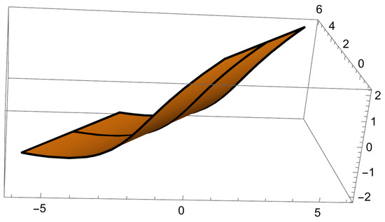
Let us consider a timelike cylindrical ruled surface in Minkowski space ${\mathbb{E}}_1^3$ with the parameter equation

$$x(s,t)=\alpha \left(s\right)+t(1,1,0),$$

where $\alpha \left(s\right)=(\sinh s,\cosh s,s)$ is a null Cartan helix (Figure 3). Its Frenet frame reads

$$\begin{array}{ccc}\hfill T\left(s\right)& =& (\cosh s,\sinh s,1),\hfill \\ \hfill N\left(s\right)& =& (\sinh s,\cosh s,0),\hfill \\ \hfill B\left(s\right)& =& -{\displaystyle \frac{1}{2}}(\cosh s,\sinh s,-1)\hfill \end{array}$$

(45)

and the curvatures are given by $k\left(s\right)=1$, $\tau \left(s\right)={\displaystyle \frac{1}{2}}$. Relation (45) yields $T\times N=T$, and hence $ϵ=1$. The Darboux frame along α has the form

$$\begin{array}{ccc}\hfill T\left(s\right)& =& (\cosh s,\sinh s,1),\hfill \\ \hfill \zeta \left(s\right)& =& (\sinh s+\cosh s,\sinh s+\cosh s,0),\hfill \\ \hfill \eta \left(s\right)& =& {\displaystyle \frac{x_s\times x_t}{\left|\right|x_s\times x_t\left|\right|}}{|}_{\alpha }=(e^s,e^s,1)\hfill \end{array}$$

(46)

It can be easily verified that $\eta \times T=-T$, so ${ϵ}_1=-1$. Because α is a null Cartan helix, by Theorems 3 and 6, it is normal helix whose axes are given by (22), (23) and (29). Substituting (45) in (22), (23) and (29) and putting ${\lambda }_0=1$, we find that axes of α are, respectively, given by

$$W_1\left(s\right)=(0,0,c_0),W_2\left(s\right)=(\tilde{c},\tilde{c},c_0),W_3\left(s\right)=(\tilde{c},\tilde{c},0).$$

By using (46), we find $k_n\left(s\right)=k_g\left(s\right)=1$. According to Theorem 12, α is an isophotic curve and a normal isophotic curve with axis $W_1$. Because the rulings of a timelike cylindrical ruled surface are parallel to $W_3$, by Theorem 9, the curve α is a silhouette with an axis $W_3$.

5. Conclusions

In this paper, we introduce a new class of null Cartan helices in Minkowski space ${\mathbb{E}}_1^3$, defined by means of a C-constant vector field $\tilde{N}$. This vector field is constant with respect to the Cartan frame, lies in the normal plane of the curve and satisfies the condition $\langle \tilde{N},W\rangle =\mathrm{constant}$, where W is a fixed axis of the helix. In this way, the concept of normal helices in Euclidean 3-space is extended to the Minkowski 3-space.

By solving a corresponding system of differential equations, we derive the necessary and sufficient conditions for a null Cartan curve to be a normal helix. Specifically, we obtain explicit expressions for the torsions of null Cartan normal helices, whether the C-constant vector field is orthogonal to the axis W or not. This analysis leads to a third-order linear homogeneous differential equation for the tangent vector field. Solving this equation in a special case yields an explicit parametric equation for the null Cartan normal helix.

A particularly noteworthy result of our study is that among all null Cartan normal helices, only the null Cartan helix admits two axes—and in a special case, even three. Furthermore, we investigate null Cartan normal helices that lie on a timelike surface and relate them to other types of curves, such as silhouettes, isophotic curves, normal silhouettes, and normal isophotic curves. We provide the necessary and sufficient conditions for these classifications, along with illustrative examples.

By using similar methods, other types of helices can be defined in Minkowski space ${\mathbb{E}}_1^3$, including null Cartan rectifying helices, null Cartan osculating helices and their spacelike and timelike counterparts. Finally, the results presented in this paper can be extended to other ambient spaces such as Galilean space ${\mathbb{G}}_3$, pseudo-Galilean space ${\mathbb{G}}_3^1$ and dual space ${\mathbb{D}}^3$.

References

- Lucas, P.; Ortega-Yagües, J.A. A generalization of the notion of helix. Turk. J. Math. 2023, 47, 1158–1168. [Google Scholar] [CrossRef]
- Dogan, F.; Yayli, Y. On isophote curves and their characterizations. Turk. J. Math. 2015, 39, 650–664. [Google Scholar] [CrossRef]
- Nešović, E.; Koç Öztürk, E.B.; Öztürk, U. On k–type null Cartan slant helices in Minkowski 3-space. Math. Meth. Appl. Sci. 2018, 41, 7583–7598. [Google Scholar] [CrossRef]
- Li, Z.; Pei, D. Null Cartan geodesic isophote curves in Minkowski 3-space. Int. J. Geom. Meth. Mod. Phys. 2024, 21, 2450142. [Google Scholar] [CrossRef]
- Djordjević, J.; Nešović, E.; Öztürk, U.; Koc Öztürk, E.B. On null Cartan normal isophotic and normal silhouette curves on a timelike surface in Minkowski 3-space. Math. Meth. Appl. Sci. 2024, 47, 10520–10539. [Google Scholar] [CrossRef]
- O’Neill, B. Semi-Riemannian Geometry with Applications to Relativity; Academic Press: San Diego, CA, USA, 1983; pp. 1–471. [Google Scholar]
- Bonnor, W.B. Null curves in a Minkowski space-time. Tensor 1969, 20, 229–242. [Google Scholar]
- Duggal, K.L.; Jin, D.H. Null Curves and Hypersurfaces of Semi–Riemannian Manifolds; World Scientific Publishing Co. Pte. Ltd.: Singapore, 2007; pp. 1–293. [Google Scholar]
- Walrave, J. Curves and Surfaces in Minkowski Space. Ph.D. Thesis, Katholieke Universiteit Leuven, Leuven, Belgium, 1995. [Google Scholar]
Disclaimer/Publisher’s Note: The statements, opinions and data contained in all publications are solely those of the individual author(s) and contributor(s) and not of MDPI and/or the editor(s). MDPI and/or the editor(s) disclaim responsibility for any injury to people or property resulting from any ideas, methods, instructions or products referred to in the content. |
© 2025 by the author. Licensee MDPI, Basel, Switzerland. This article is an open access article distributed under the terms and conditions of the Creative Commons Attribution (CC BY) license (https://creativecommons.org/licenses/by/4.0/).