Opposition and Implication in Aristotelian Diagrams

Abstract

In logical geometry, Aristotelian diagrams are studied in a systematic fashion. Recent developments in this field have shown that the square of opposition generalizes in two ways, which correspond precisely to the theory of opposition (leading to $\alpha$-structures) and the theory of implication (leading to ladders) it exhibits. These two kinds of Aristotelian diagrams are dual to each other, in the sense that they are the oppositional and implicative counterpart of the same construction. This paper formalizes this duality as $OI$-companionship, explores its properties, and applies it to various $\sigma$-diagrams. This investigation shows that $OI$-companionship has some interesting, but unusual behaviors. While it is symmetric, and works well on the level of Aristotelian families, it lacks (ir)reflexivity, transitivity, functionality, and seriality. However, we show that all important Aristotelian families from the literature do have a unique $OI$-companion. These findings explore the limits that arise when extending the duality between opposition and implication beyond the limits of $\alpha$-structures and ladders.

1. Introduction

Aristotelian diagrams, such as the square of opposition [1], consist of a number of sentences and certain logical relations holding between them. The most important of these relations are those of contradiction, contrariety, subcontrariety, and subalternation. There is a well-known discrepancy among these relations: while the first three are defined in terms of whether the formulas can be true/false together, the last one is defined in terms of logical entailment. This basic observation has led Smessaert and Demey to distinguish between opposition relations on the one hand, and implication relations on the other [2,3]. This has the conceptual advantage that every pair of formulas stands in exactly one opposition relation and exactly one implication relation. Historically speaking, Correia [4] has argued that the square of opposition represents both a theory of negation (which explains its occurrence in commentaries on Aristotle’s On Interpretation) as well as a theory of inference (which explains its occurrence in commentaries on the Prior Analytics). This double role maps nicely onto the distinction between opposition and implication relations, respectively. Because of these deep conceptual and historical roots that opposition and inference have within Aristotelian diagrams, any comprehensive treatment of Aristotelian diagrams must pay close attention to how both of these theories behave. For example, we will introduce the notions of $OI$-map and $OI$-companionship between Aristotelian diagrams, which allows us to formally capture Correia’s claims about the square of opposition.

In addition to such conceptual and historical considerations, these relations are also important from a contemporary mathematical perspective on Aristotelian diagrams [5,6,7,8,9,10]. In fact, recent work in logical geometry [11,12] (i.e., the research endeavour in which these diagrams are studied in a systematic and mathematically sophisticated way) has shown that Aristotelian diagrams can be fruitfully studied using the machinery of category theory, and the notion of morphism required to facilitate this investigation is based on opposition and implication relations [13]. Similarly, these two types of relations play a crucial role in studying two different types of generalizations of the square of opposition, viz., $\alpha$-structures and ladders, respectively [14]. The $\alpha$-structures, which are defined in terms of opposition relations, can be viewed as a generalization of the theory of negation that resides within the square of opposition. The ladders, which are defined in terms of implication relations, generalize the theory of inference that is exhibited by the square.

An important recent discovery in logical geometry is that $\alpha$-structures and ladders are dual to each other, in the sense that they are the oppositional and implicative counterparts of the same kind of construction (pp. 19–20, [14]). The main aim of this paper is to introduce and investigate the notion of $OI$-companionship. This notion is meant to generalize this idea of duality in such a way that it can be applied to any kind of Aristotelian diagram.

The insights of logical geometry are being applied to an ever increasingly wide variety of disciplines, within and outside of philosophy and logic, which already includes (but is not at all limited to) epistemology [15,16], ethics [17,18,19], probabilistic and fuzzy logics [20,21], pragmatics [22,23,24,25,26], neuroscience [27,28], computer science [29,30,31,32], psychology [33,34,35], and natural language processing [36,37]. Additionally, even authoritative reference works for the aforementioned disciplines often contain Aristotelian diagrams [38,39,40,41]. To warrant the quality of these applications, it is of the utmost importance that the framework of logical geometry is well understood. In particular, both the theory of negation and that of inference, which lie at the heart of the square of opposition and its extensions [3,4,13,14], must be thoroughly investigated. This is why it is essential that we grasp the fundamental properties of the notion of $OI$-companionship, so that it becomes more clear how both of these theories are interconnected.

This paper is structured as follows: We start by going over the necessary preliminaries from logical geometry in Section 2. Then, we introduce the notion of $OI$-companionship in Section 3, while also looking at its key properties. In Section 4, we go through the different kinds of $\sigma$-diagrams (which are the most important Aristotelian diagrams) up to an acceptable size, and discuss all of their $OI$-companions. We also make up an overview of the concrete findings and comment on the patterns and unusual behaviors that we find. These unusual behaviors are looked at more closely in Section 5, where we prove that the relation of $OI$-companionship is neither reflexive, nor transitive, nor functional, nor serial. In particular, this means that Aristotelian families can have 0, 1, or more $OI$-companions. Finally, in Section 6, we wrap things up and give some thoughts on future research.

2. Background on Logical Geometry

Logical geometry concerns itself with the systematic study of Aristotelian diagrams. However, these diagrams have been circulating since Antiquity, and it is therefore not surprising that there are different perspectives that one can take when studying them. These different perspectives translate to a variety of possible definitions of Aristotelian diagrams, some of which are more general than others [42]. In this paper, we adopt the most general perspective to date, which uses the setting of Boolean algebra. For an extensive introduction to the theory behind Boolean algebra, we refer to [43].

Definition 1. 

An Aristotelian diagram D is a pair $(\mathcal{F},B)$, where B is a Boolean algebra $(B,{\wedge }_B,{\vee }_B,{\neg }_B,1_B,0_B)$ and $\mathcal{F}$ is a fragment of B, i.e., $\mathcal{F}\subseteq B$. Furthermore, a σ-diagram is an Aristotelian diagram $(\mathcal{F},B)$ such that $\mathcal{F}$ is closed under ${\neg }_B$, i.e., for all $x\in \mathcal{F}$, we have ${\neg }_{B}x\in \mathcal{F}$ as well. When the Boolean algebra B is clear from context, it is usually omitted as a subscript to ∧, ∨, etc.

Definition 1 clearly states that Aristotelian diagrams are made up of Boolean algebras B and their subsets $\mathcal{F}$. From a naive point of view, one might say that such a definition is not suitable for a kind of diagram, since it does not refer to visualizations in any way. However, an analogy with the case of graphs in mathematics is already enough to justify this way of defining Aristotelian diagrams. Indeed, even though graphs are accepted in the mathematical community as visualizations of networks, they are still defined as couples containing a set of vertices and a set of edges [44].

In an Aristotelian diagram $(\mathcal{F},B)$, we want to visualize certain relations that hold between the elements of $\mathcal{F}$ inside the Boolean algebra B. More concretely, the relations in question are called the Aristotelian relations, and they can be defined as follows:

Definition 2. 

Given a Boolean algebra B, we say that $x,y\in B$ are:

• B-contradictory (${\mathit{CD}}_B$) iff $x{\wedge }_{B}y=0_B$ and $x{\vee }_{B}y=1_B$,
• B-contrary (${\mathit{C}}_B$) iff $x{\wedge }_{B}y=0_B$ and $x{\vee }_{B}y\ne 1_B$,
• B-subcontrary (${\mathit{SC}}_B$) iff $x{\wedge }_{B}y\ne 0_B$ and $x{\vee }_{B}y=1_B$,
• in B-subalternation (${\mathit{SA}}_B$) iff ${\neg }_{B}x{\vee }_{B}y=1_B$ and $x{\vee }_B{\neg }_{B}y\ne 1_B$.

These four relations are called the Aristotelian relations for B; we also write ${\mathcal{AR}}_B:=\{{\mathit{CD}}_B,{\mathit{C}}_B,{\mathit{SC}}_B,{\mathit{SA}}_B\}$. When no confusion is possible, B is usually omitted as a prefix and subscript. We follow a commonly used visualization convention in logical geometry, in which contradiction is depicted by a solid line, contrariety by a dashed line, subcontrariety by a dotted line, and subalternation by an arrow.

The idea of defining Aristotelian diagrams in the context of Boolean algebras is a quite recent development [42]. Historically speaking, these diagrams were usually defined in the context of logic [1]. However, with the use of Lindenbaum–Tarski algebras, it is not hard to see that the former is simply a generalization of the latter (pp. 4–5, [13]). This generalization allows us to use bitstring semantics, a highly effective tool for systematically studying the properties of Aristotelian diagrams [5,45]. With this development in mind, it is appropriate that we now turn to an example from logic (Example 1), and an example that uses bitstrings (Example 2).

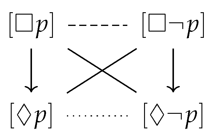
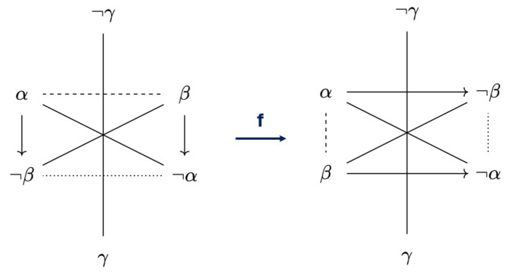
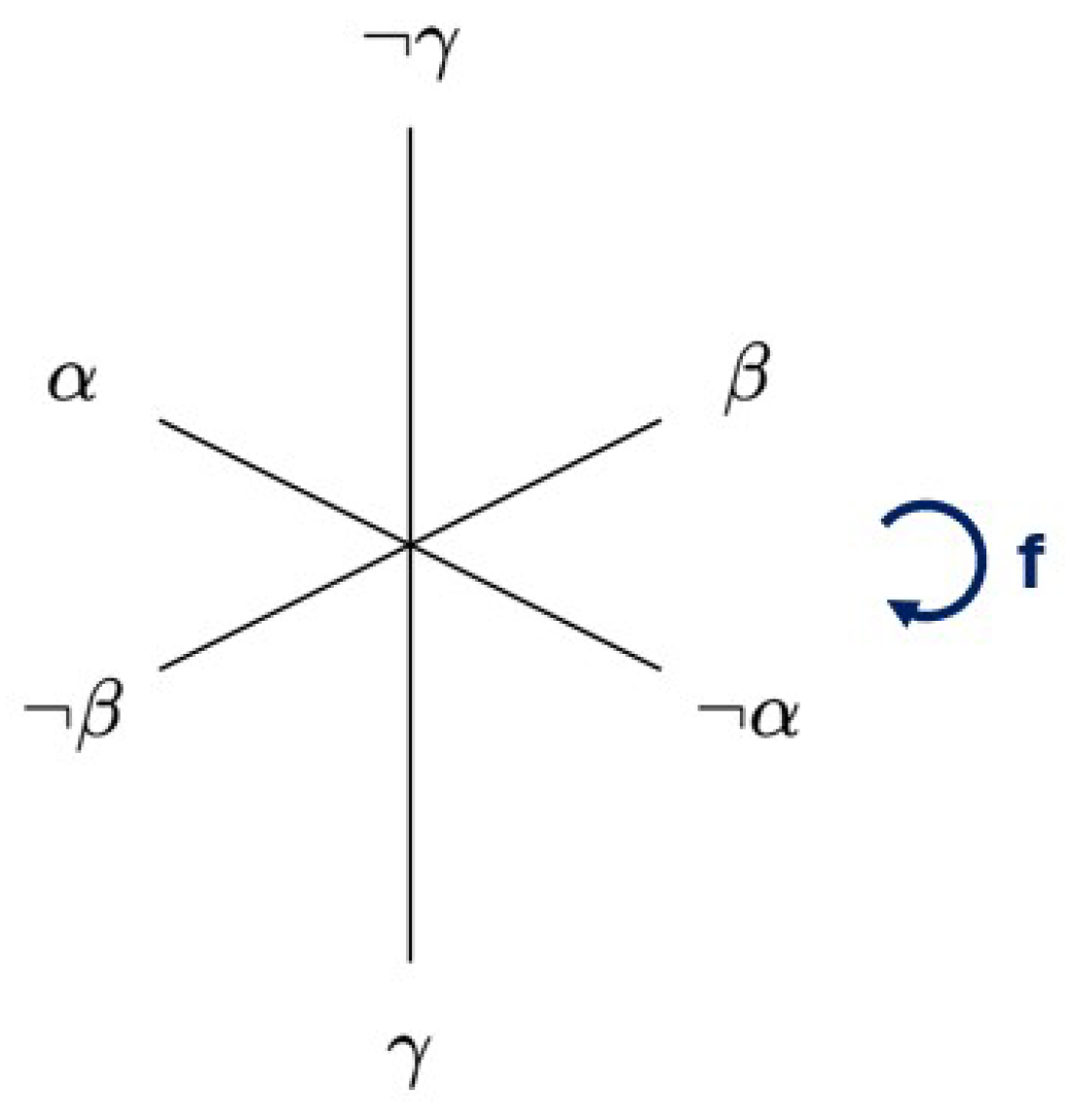
Example 1. 

Since the modal logic $\mathsf{KD}$ has Boolean operators, its Lindenbaum–Tarski algebra $\mathbb{B}\left(\mathsf{KD}\right)$ is a Boolean algebra. Let us now consider the fragment $\mathcal{F}=\left\{\right[\square p],[◊p],[\square \neg p],[◊\neg p\left]\right\}$ inside $\mathbb{B}\left(\mathsf{KD}\right)$. Here, the square brackets indicate that the elements of $\mathbb{B}\left(\mathsf{KD}\right)$ are equivalence classes of formulas with respect to logical equivalence in $\mathsf{KD}$. Drawing the Aristotelian relations that hold between each pair of elements of $\mathcal{F}$, we can visualize $(\mathcal{F},\mathbb{B}(\mathsf{KD}\left)\right)$ as in Figure 1. An Aristotelian diagram that looks like this is commonly known as a square of opposition.

Example 2. 

Let $B={\{0,1\}}^4$ be a bitstring algebra, and let ${\mathcal{F}}_1$ be the fragment

$${\mathcal{F}}_1:=\{1000,0100,0001,1110,1011,0111\}$$

inside B. We can then visualize the Aristotelian diagram $({\mathcal{F}}_1,B)$ as in the left of Figure 2, which is commonly known as a (weak) Jacoby–Sesmat–Blanché (JSB) hexagon, or as a weak ${\alpha }_3$-structure. In the same Boolean algebra, let ${\mathcal{F}}_2$ be the fragment

$${\mathcal{F}}_2:=\{1000,1100,1110,0001,0011,0111\}.$$

We can visualize the Aristotelian diagram $({\mathcal{F}}_2,B)$ as in the right of Figure 2, which is commonly known as a Sherwood–Czeżowski (SC) hexagon, or as a 3-ladder. It is drawn in a somewhat unorthodox way to highlight the similarities with the JSB hexagon to its left. These similarities will be made precise by Proposition 1 below. For more details on unorthodox ways of drawing Aristotelian diagrams, see [46].

As described in Section 1, there is a clear discrepancy among the four Aristotelian relations, which can be observed in Definition 2. The relations of contradiction, contrariety, and subcontrariety are defined in a very similar way, namely, in terms of whether or not the identities $x\wedge y=0$ and $x\vee y=1$ hold between the elements x and y they connect. In a Lindenbaum–Tarski algebra B, we always have that 0 and 1 are equal to $[\perp ]$ and $[\top ]$, and therefore, these three relations determine whether or not two formulas can be true/false at the same time. Additionally, it is easy to see that in Lindenbaum–Tarski algebras, there is a one-way entailment from one formula to the other precisely when there is a subalternation between them in the same direction.

This dichotomy between contradiction, contrariety, and subcontrariety on the one hand, and subalternation on the other, suggests that Aristotelian diagrams should not be viewed as visualizations of a single structure. Rather, they visualize both an oppositional structure and an implicative structure together. These considerations fueled Smessaert and Demey to investigate these oppositional and implicative structures as separate entities, which come together in Aristotelian diagrams [3]. A major breakthrough in this investigation was the discovery of the opposition and implication relations, which is a set of 8 relations that contains all of the Aristotelian relations.

Definition 3. 

Given a Boolean algebra B, we say that $x,y\in B$ are:

• B-contradictory (${\mathit{CD}}_B$) iff $x{\wedge }_{B}y=0_B$ and $x{\vee }_{B}y=1_B$ (i.e., $x={\neg }_{B}y$),
• B-contrary (${\mathit{C}}_B$) iff $x{\wedge }_{B}y=0_B$ and $x{\vee }_{B}y\ne 1_B$ (i.e., $x{<}_B{\neg }_{B}y$),
• B-subcontrary (${\mathit{SC}}_B$) iff $x{\wedge }_{B}y\ne 0_B$ and $x{\vee }_{B}y=1_B$ (i.e., $x{>}_B{\neg }_{B}y$),
• B-non-contradictory (${\mathit{NCD}}_B$) iff $x{\wedge }_{B}y\ne 0_B$ and $x{\vee }_{B}y\ne 1_B$,
• in B-bi-implication (${\mathit{BI}}_B$) iff $x{\le }_{B}y$ and $x{\ge }_{B}y$ (i.e., $x=y$),
• in B-left-implication (${\mathit{LI}}_B$) iff $x{\le }_{B}y$ and $x{\ngeqq }_{B}y$ (i.e., $x{<}_{B}y$),
• in B-right-implication (${\mathit{RI}}_B$) iff $x{\nleqq }_{B}y$ and $x{\ge }_{B}y$ (i.e., $x{>}_{B}y$),
• in B-non-implication (${\mathit{NI}}_B$) iff $x{\nleqq }_{B}y$ and $y{\ngeqq }_{B}x$.

The first four relations are called the opposition relations for B and the last four are called the implication relations for B. We also write ${\mathcal{OR}}_B:=\{{\mathit{CD}}_B,{\mathit{C}}_B,{\mathit{SC}}_B,{\mathit{NCD}}_B\}$ and ${\mathcal{IR}}_B:=\{{\mathit{BI}}_B,{\mathit{LI}}_B,{\mathit{RI}}_B,{\mathit{NI}}_B\}$. When x and y are both B-non-contradictory and in B-non-implication, we say that they are B-unconnected. When no confusion is possible, B is usually omitted as a prefix and subscript.

Let us now revisit Example 2. Looking at Figure 2; we can see some similarities between the JSB hexagon on the left, and the SC hexagon on the right. The former has two interlocking triangles of opposition relations (C and $SC$) on the inside and only implication relations on the outside ($LI$ and $RI$), while the latter has two interlocking triangles of implication relations ($LI$ and $RI$) on the inside and only opposition relations (C and $SC$) on the outside. It thus seems like the roles of opposition on implication have switched. However, this is not entirely true, because all of the contradiction and bi-implication relations are in exactly the same place in both Aristotelian diagrams. These observations have been made precise in (pp. 19–20, [14]), with the aid of the following auxiliary notions.

Definition 4. 

Let B be a Boolean algebra. We define ${\mathcal{R}}_B$ as the set of relations on B given by ${\mathcal{R}}_B:=\{{\mathit{CD}}_B,{\mathit{C}}_B\cup {\mathit{SC}}_B,{\mathit{BI}}_B,L{I}_B\cup R{I}_B\}$. Let $B^{\prime }$ be another Boolean algebra. We define the function $F_B^{B^{\prime }}:{\mathcal{R}}_B\to {\mathcal{R}}_{B^{\prime }}$ pointwise as follows:

$$\begin{array}{cc}\hfill F_B^{B^{\prime }}\left(C{D}_B\right)& :=C{D}_{B^{\prime }},\hfill \\ \hfill F_B^{B^{\prime }}\left(B{I}_B\right)& :=B{I}_{B^{\prime }},\hfill \\ \hfill F_B^{B^{\prime }}(C_B\cup S{C}_B)& :=L{I}_{B^{\prime }}\cup R{I}_{B^{\prime }},\hfill \\ \hfill F_B^{B^{\prime }}(L{I}_B\cup R{I}_B)& :=C_{B^{\prime }}\cup S{C}_{B^{\prime }}.\hfill \end{array}$$

When no confusion is possible, we omit the sub-/superscripts B and $B^{\prime }$.

The similarity between JSB hexagons and SC hexagons as described above extends to a similarity between the series of ${\alpha }_n$-structures and the series of n-ladders. To make sure this paper is relatively self-contained, we incorporate the definitions of both of these series here. They are taken from [14].

Definition 5. 

Let $n\in {\mathbb{N}}_0$ be a natural number. An ${\alpha }_n$-structure is a σ-diagram $(\mathcal{F},B)$ such that

• $\left|\mathcal{F}\right|=2n$,
• $0_B,1_B\notin \mathcal{F}$ and
• $\exists X\subseteq \mathcal{F}$ such that $\left|X\right|=n$ and ${\mathit{C}}_B(a,b)$ for all distinct $a,b\in X$.

Dropping reference to the specific number of elements, any ${\alpha }_n$-structure is more generally called an α-structure.

Definition 6. 

Let $n\in {\mathbb{N}}_0$ be a natural number. An n-ladder is a σ-diagram $(\mathcal{F},B)$ such that

• $\left|\mathcal{F}\right|=2n$,
• $0_B,1_B\notin \mathcal{F}$ and
• $\exists y=(y_1,\dots ,y_n)\in {\mathcal{F}}^n$ such that ${\mathit{LI}}_B(y_i,y_{i+1})$ for all $1\le i\le n-1$.

Dropping reference to the specific number of elements, any n-ladder is more generally called a ladder.

Essentially, the similarity between $\alpha$-structures and ladders as described above is captured by Proposition 1 below, which is a weaker version of Proposition 4 from [14]. The difference between these two propositions is that the latter includes the construction of f in the statement of the proposition, while the former merely states that some appropriate bijection f exists. This simplification has the advantage of focusing on the essence of the similarity between $\alpha$-structures and ladders, the only part that is necessary to create the generalization that will be studied in the remainder of this paper. Additionally, we do not really lose anything here, since the construction of f can still be found in the proof of Proposition 1.

Proposition 1. 

Let $n\in {\mathbb{N}}_0$ be a natural number, let $D=(\mathcal{F},B)$ be an ${\alpha }_n$-structure, and let $D^{\prime }=({\mathcal{F}}^{\prime },B^{\prime })$ be an n-ladder. Then, there exists a bijection $f:\mathcal{F}\to {\mathcal{F}}^{\prime }$ such that for all $R\in {\mathcal{R}}_B$ and $x,y\in \mathcal{F}$, we have that

$$R(x,y)\iff F_B^{B^{\prime }}\left(R\right)(f\left(x\right),f\left(y\right)).$$

Proof. 

This follows immediately from Proposition 4 from [14], but we sketch how f can be constructed here as well. Let X be the set of n pairwise contrary elements in $\mathcal{F}$, let $(y_1,\dots ,y_n)$ be a tuple with elements in ${\mathcal{F}}^{\prime }$ such that ${\mathit{LI}}_B(y_i,y_{i+1})$ for all $1\le i\le n-1$, and let $Y:=\{y_1,\dots y_n\}$. Then, f can be any negation-preserving bijection such that $f\left(X\right)=Y$. □

Proposition 1 helps to shed some light on why $\mathcal{R}$ and F are defined in the way that they are. Notice that the relations C and $SC$ are symmetric (i.e., $C(x,y)$ if, and only if, $C(y,x)$), while $LI$ and $RI$ are not. Even more so, it holds that $LI(x,y)$ if, and only if, $RI(y,x)$. This means that, if an instance of C between x and y is transformed into an instance of $LI$ between $f\left(x\right)$ and $f\left(y\right)$, then the instance of C between y and x will be transformed into the instance of $RI$ between $f\left(y\right)$ and $f\left(x\right)$. Therefore, it is not possible to transform all instances of C into instances of $LI$, because half of them will automatically be transformed into instances of $RI$. In particular, it now becomes clear why C and $SC$, as well as $LI$ and $RI$, are combined into two unions in the definitions of $\mathcal{R}$ and F.

Because of Proposition 1, one might be inclined to think that Definition 4 should also require that $F_B^{B^{\prime }}\left(NC{D}_B\right):=NC{D}_{B^{\prime }}$ and $F_B^{B^{\prime }}\left(N{I}_B\right):=N{I}_{B^{\prime }}$. However, this would be misguided, since we want to preserve some flexibility in regards to $NCD$ and $NI$. On the one hand, we want to be able to preserve them in certain cases. For example, when two elements x and y are unconnected, we want their images under the bijection f to be unconnected as well. On the other hand, we want to be able to discard instances of $NCD$ and $NI$ in certain cases. For instance, in Example 2, every (sub)contrariety relation coincides with an instance of $NI$, and every subalternation relation coincides with an instance of $NCD$. When we have, for two elements x and y, that $C(x,y)$, we want their images under f to be subalternated, which would make the instance of $NI$ between them disappear.

Finally, an important notion from contemporary logical geometry is that of an Aristotelian isomorphism. Informally, it determines whether two Aristotelian diagrams enter into exactly the same constellation of Aristotelian relations, i.e., whether their visualizations can give the same figure. The formal definition adopts an auxiliary notion, namely, the relabel function ${\mathsf{ı}}_B^{B^{\prime }}$, which identifies all relations in B with their counterparts in $B^{\prime }$ [13].

Definition 7. 

Let B and $B^{\prime }$ be Boolean algebras. We define the relabel function ${\mathsf{ı}}_B^{B^{\prime }}:{\mathcal{OR}}_B\cup {\mathcal{IR}}_B\to {\mathcal{OR}}_{B^{\prime }}\cup {\mathcal{IR}}_{B^{\prime }}$ from B to $B^{\prime }$ as

$$\begin{array}{cc}{\mathsf{ı}}_B^{B^{\prime }}\left({\mathit{CD}}_B\right):={\mathit{CD}}_{B^{\prime }};& {\mathsf{ı}}_B^{B^{\prime }}\left({\mathit{BI}}_B\right):={\mathit{BI}}_{B^{\prime }};\\ {\mathsf{ı}}_B^{B^{\prime }}\left(C_B\right):=C_{B^{\prime }};& {\mathsf{ı}}_B^{B^{\prime }}\left({\mathit{LI}}_B\right):={\mathit{LI}}_{B^{\prime }};\\ {\mathsf{ı}}_B^{B^{\prime }}\left({\mathit{SC}}_B\right):={\mathit{SC}}_{B^{\prime }};& {\mathsf{ı}}_B^{B^{\prime }}\left({\mathit{RI}}_B\right):={\mathit{RI}}_{B^{\prime }};\\ {\mathsf{ı}}_B^{B^{\prime }}\left({\mathit{NCD}}_B\right):={\mathit{NCD}}_{B^{\prime }};& {\mathsf{ı}}_B^{B^{\prime }}\left({\mathit{NI}}_B\right):={\mathit{NI}}_{B^{\prime }}.\end{array}$$

When no confusion is possible, we omit the sub-/superscripts B and $B^{\prime }$.

Definition 8. 

Let $D=(\mathcal{F},B)$ and $D^{\prime }=({\mathcal{F}}^{\prime },B^{\prime })$ be Aristotelian diagrams. We say that $f:\mathcal{F}\to {\mathcal{F}}^{\prime }$ is an Aristotelian isomorphism from D to $D^{\prime }$ iff f is bijective and for all Aristotelian relations $R\in {\mathcal{AR}}_B$ and $x,y\in \mathcal{F}$, we have

$$R(x,y)\iff {\mathsf{ı}}_B^{B^{\prime }}\left(R\right)(f\left(x\right),f\left(y\right)).$$

If such an f exists, we also say that D and $D^{\prime }$ are Aristotelian isomorphic.

Being Aristotelian isomorphic is an equivalence relation on the class of all Aristotelian diagrams. The equivalence classes of this relation are called Aristotelian families. It is worth noting that these Aristotelian isomorphisms are also isomorphisms in the sense of category theory. Indeed, one can define multiple kinds of morphisms between Aristotelian diagrams that give rise to categories in which the isomorphisms are precisely the Aristotelian isomorphisms from Definition 8 [13]. Two of these categories, namely, ${\mathbb{D}}_{\mathcal{OR}\times \mathcal{IR}}^{Inc}$ and ${\mathbb{D}}_{\mathcal{OR}\times \mathcal{IR}}^{Dec}$, are currently under investigation in a book-length study that goes to a deeper level of category theory [47].

3. What OI-Companionship Is

In this section, we define the central notion of this paper, namely, $OI$-companionship, and discuss its core properties. It is a relation that can hold between different (families of) Aristotelian diagrams, inspired by the similarities between $\alpha$-structures and ladders from Proposition 1. Without further ado, let us state the definition of $OI$-companionship between two Aristotelian diagrams.

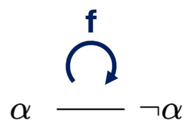
Definition 9. 

Let $D=(\mathcal{F},B)$ and $D^{\prime }=({\mathcal{F}}^{\prime },B^{\prime })$ be Aristotelian diagrams. We say that $f:\mathcal{F}\to {\mathcal{F}}^{\prime }$ is an $OI$-map from D to $D^{\prime }$ iff f is bijective and for all $R\in {\mathcal{R}}_B$ and $x,y\in \mathcal{F}$, we have that

$$R(x,y)\iff F_B^{B^{\prime }}\left(R\right)(f\left(x\right),f\left(y\right)).$$

If such an f exists, we also say that D and $D^{\prime }$ are $OI$-companions.

Before we go any further, let us clarify, to avoid any confusion, that the above definition uses the set of relations $\mathcal{R}$ from Definition 4, and none of the sets $\mathcal{AR},\mathcal{OR}$, or $\mathcal{IR}$ from Definitions 2 and 3. Let us start by making some immediate remarks. Notice first of all that Definition 9 allows us to rephrase Proposition 1 in a very neat way, which is stated in Corollary 1 below.

Corollary 1. 

Let $n\in {\mathbb{N}}_0$ be a natural number, let D be an ${\alpha }_n$-structure and let $D^{\prime }$ be an n-ladder. Then, D and $D^{\prime }$ are $OI$-companions.

Proof. 

This can be seen immediately from Proposition 1 and Definition 9. □

Secondly, comparing Definitions 8 and 9, we find a strong resemblance between Aristotelian isomorphisms and $OI$-maps. The only difference is that the former uses $\mathcal{AR}$ and the relabel maps ${\mathsf{ı}}_B^{B^{\prime }}$, while the latter uses $\mathcal{R}$ and the maps $F_B^{B^{\prime }}$. This strong resemblance is due to the fact that both notions compare two Aristotelian diagrams on the level of their constellation of Aristotelian relations. Thirdly, it is important to keep in mind that the function f from Definition 9 must be a bijection. This means that we have a very simple necessary condition for two Aristotelian diagrams to be $OI$-companions: their fragments must be of the same size. Finally, it is worth noting that $OI$-companionship is framed in a symmetric way in Definition 9. If an $OI$-map $f:D\to D^{\prime }$ exists, then D and $D^{\prime }$ are said to be each other’s $OI$-companion, which, in turn, would mean that an $OI$-map $g:D^{\prime }\to D$ exists. This last point is justified by Proposition 2 below.

Proposition 2. 

Let $D=(\mathcal{F},B)$ and $D^{\prime }=({\mathcal{F}}^{\prime },B^{\prime })$ be Aristotelian diagrams, and let $f:\mathcal{F}\to {\mathcal{F}}^{\prime }$ be an $OI$-map from D to $D^{\prime }$. Then, $f^{-1}$ is an $OI$-map from $D^{\prime }$ to D. Therefore, $OI$-companionship is a symmetric relation on the class of all Aristotelian diagrams.

Proof. 

Since f is bijective, it is immediate that $f^{-1}$ is a well-defined bijection from ${\mathcal{F}}^{\prime }$ to $\mathcal{F}$. The crucial observation here, which can be seen straight from Definition 4, is that $F_B^{B^{\prime }}$ is a bijective function and we have that ${\left(F_B^{B^{\prime }}\right)}^{-1}=F_{B^{\prime }}^B$. Using this simple observation, we obtain, for all $x^{\prime },y^{\prime }\in {\mathcal{F}}^{\prime }$ and all $R^{\prime }\in {\mathcal{R}}_{B^{\prime }}$, that

$$\begin{array}{cc}\hfill R^{\prime }(x^{\prime },y^{\prime })& \iff F_B^{B^{\prime }}\left(F_{B^{\prime }}^B\left(R^{\prime }\right)\right)(f\left(f^{-1}\left(x^{\prime }\right)\right),f\left(f^{-1}\left(y^{\prime }\right)\right))\hfill \\ \hfill & \iff F_{B^{\prime }}^B\left(R^{\prime }\right)(f^{-1}\left(x^{\prime }\right),f^{-1}\left(y^{\prime }\right)),\hfill \end{array}$$

where the second equivalence follows from the assumption that f is an $OI$-map. □

Let us now look back at Corollary 1, which captures the insight from Proposition 4 of [14] in a precise way. Essentially, this is quite a strong result, since it is not just about two individual diagrams, but rather about two entire Aristotelian families. In particular, this result suggests that it makes sense to lift the relation of $OI$-companionship from the class of all Aristotelian diagrams to the class of all Aristotelian families.

Definition 10. 

Let $\mathcal{D}$ and ${\mathcal{D}}^{\prime }$ be Aristotelian families. If for all $D\in \mathcal{D}$, and all $D^{\prime }\in {\mathcal{D}}^{\prime }$, it holds that D and $D^{\prime }$ are $OI$-companions, we say that $\mathcal{D}$ and ${\mathcal{D}}^{\prime }$ are $OI$-companions.

Corollary 2. 

Let $n\in {\mathbb{N}}_0$ be a natural number. Then, the family of ${\alpha }_n$-structures and the family of n-ladders are $OI$-companions.

Proof. 

This follows immediately from Definition 10 and Corollary 1. □

Of course, $OI$-companionship between Aristotelian families would not be an interesting notion if its only instances were between the ${\alpha }_n$-structures and the n-ladders, for every $n\in {\mathbb{N}}_0$. Therefore, it is a satisfactory result that all instances of $OI$-companionship between individual diagrams automatically give rise to $OI$-companionship between their respective Aristotelian families, as Proposition 3 below shows.

Proposition 3. 

Let $D=(\mathcal{F},B),D^{\prime }=({\mathcal{F}}^{\prime },B^{\prime })$, and $D^{\prime \prime }=({\mathcal{F}}^{\prime \prime },B^{\prime \prime })$ be Aristotelian diagrams such that D and $D^{\prime }$ are Aristotelian isomorphic. If $D^{\prime }$ and $D^{\prime \prime }$ are $OI$-companions, then so are D and $D^{\prime \prime }$.

Proof. 

Let $f_1:\mathcal{F}\to {\mathcal{F}}^{\prime }$ be an Aristotelian isomorphism from D to $D^{\prime }$, and let $f_2:{\mathcal{F}}^{\prime }\to {\mathcal{F}}^{\prime \prime }$ be an $OI$-map from $D^{\prime }$ to $D^{\prime \prime }$. It then follows immediately from Definitions 8 and 9 that $f_2\circ f_1$ is an $OI$-map from D to $D^{\prime \prime }$, and thus $D^{\prime \prime }$ is an $OI$-companion of D. □

Corollary 3. 

Let $\mathcal{D}$ and ${\mathcal{D}}^{\prime }$ be Aristotelian families, and let $D\in \mathcal{D}$, and $D^{\prime }\in {\mathcal{D}}^{\prime }$. Then, we have that D and $D^{\prime }$ are $OI$-companions if, and only if, $\mathcal{D}$ and ${\mathcal{D}}^{\prime }$ are $OI$-companions.

Proof. 

This follows immediately from Definition 10 and Propositions 2 and 3. □

This final corollary makes it very precise that we do not need to discuss $OI$-companionship between individual diagrams and between entire families separately, since they will have virtually the same properties. Therefore, in the remainder of this paper, whenever we do not specify which kind of $OI$-companionship is under consideration, it means that the discussion applies to both of them.

4. Examples of OI-Companionship

We now proceed to go through some examples of Aristotelian families and their $OI$-companions. Of course, we are primarily concerned with those families that have been used and studied the most in the literature, as opposed to those that might be less useful for other research enterprises. Therefore, we restrict our attention to (families of) $\sigma$-diagrams (see Definition 1) that have a small fragment $\mathcal{F}$, and do not contain the top and bottom elements 1 and 0 of the ambient Boolean algebra B. More precisely, we go over all possible cases for $\left|\mathcal{F}\right|=2n$, where $n\in \{1,2,3,4\}$. We will use the size of the fragment $\left|\mathcal{F}\right|$ as a way of ordering these examples from smaller to larger.

Let us start with the smallest possible value of $\left|\mathcal{F}\right|$, which is 2. In this case, there is just a single Aristotelian family, which is the family of PCDs (Pairs of Contradictories). Because of Corollary 3, the specific Boolean algebra and fragment in question do not matter all that much. Therefore, we resort to using Greek letters to indicate that we consider generic Aristotelian diagrams, which are allowed to be any specific diagram in any Boolean algebra [48].

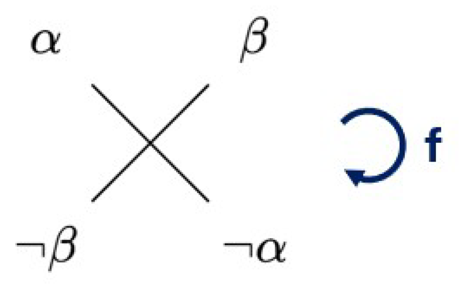
Example 3. 

Let us consider a (generic) PCD, as in Figure 3. Since it contains no contrariety, subcontrariety, or left- or right-implication relations, it is immediately clear that it has a unique (up to Aristotelian isomorphism of course) $OI$-companion, which is itself. In particular, both bijections from $\{\alpha ,\neg \alpha \}$ to itself are $OI$-maps, and can be used as f in Figure 3. Because of Corollary 3, we can now say that the family of PCDs is its own $OI$-companion.

Increasing the fragment size $\left|\mathcal{F}\right|$ from 2 to 4, we have the next smallest $\sigma$-diagrams, which contain 2 PCDs. These diagrams are usually drawn in such a way that these two PCDs form the diagonals of a square, so that negation coincides with central symmetry [49]. Therefore, they are often called squares. There are exactly two Aristotelian families in this case [50], namely, the family of classical squares of opposition and that of degenerate squares, which are considered in the following examples.

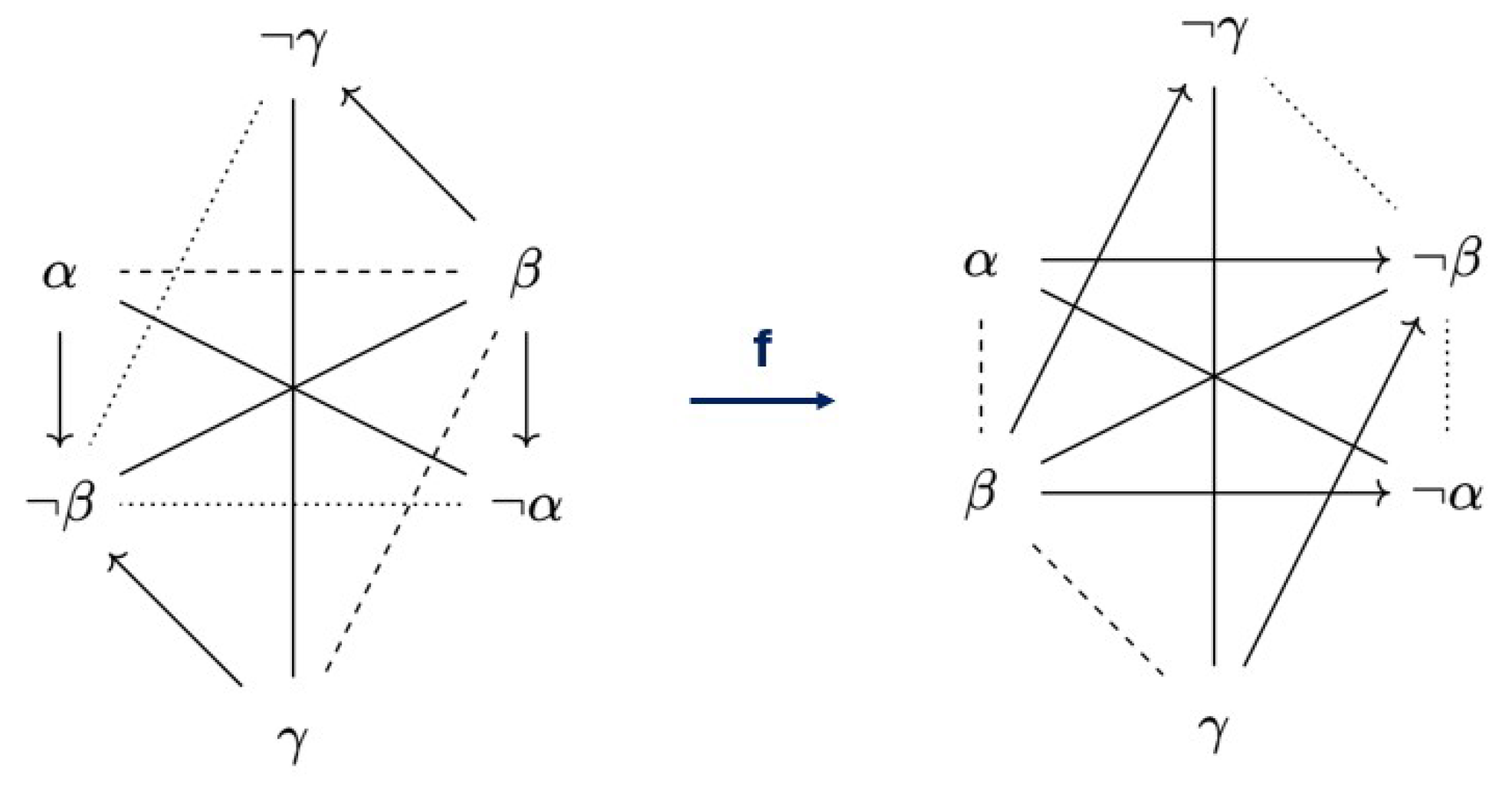
Example 4. 

Let us consider a (generic) classical square of opposition D, as in the left of Figure 4. It is not hard to construct an $OI$-map f from this diagram to itself. For example, we can set

$$\begin{array}{cc}\hfill f\left(\alpha \right)& :=\alpha ,\hfill \\ \hfill f(\neg \alpha )& :=\neg \alpha ,\hfill \\ \hfill f\left(\beta \right)& :=\neg \beta ,\hfill \\ \hfill f(\neg \beta )& :=\beta .\hfill \end{array}$$

This map f is visualized in Figure 4, from which it can be checked that it really is an $OI$-map. Therefore, D is its own $OI$-companion. Since D is both an ${\alpha }_2$-structure and a 2-ladder, this result also follows immediately from Corollary 1. By Corollary 2, we can also say that the family of squares of opposition is its own $OI$-companion. One can notice that f is by no means unique, it is just one of the possible $OI$-maps from D to itself. On a more important note, it is not hard to prove that D has (up to Aristotelian isomorphism) no other $OI$-companions. Indeed, since $OI$-maps are bijective and must preserve contradictions, the only other candidate would be the degenerate squares from Example 5, but these contain no Aristotelian relations other than contradiction.

Example 5. 

Let us consider a (generic) degenerate square D, as in Figure 5. It is almost trivial to construct an $OI$-map f from this diagram to itself. For example, we can simply use the identity map on its fragment. Therefore, D is its own $OI$-companion. Because of Corollary 3, we can now say that the family of degenerate squares is its own $OI$-companion. Again, f is by no means unique, it is just one of the possible $OI$-maps from D to itself. More importantly, it is not hard to prove that D has (up to Aristotelian isomorphism) no other $OI$-companions. Indeed, since $OI$-maps are bijective and must preserve contradictions, the only other candidate would be the classical squares of opposition from Example 4, but these contain Aristotelian relations that cannot be found in D.

Increasing the fragment size $\left|\mathcal{F}\right|$ once again, this time from 4 to 6, we have the next smallest $\sigma$-diagrams, which contain three PCDs, and are often called hexagons. There are exactly five Aristotelian families in this case [50], namely, the JSB hexagons and the SC hexagons from Example 2, and the U4, U8, and U12 hexagons (named after the number of occurrences of unconnectedness from Definition 3), which are all considered in the following series of examples.

Example 6. 

Let us consider a (generic) JSB hexagon D, as in the left of Figure 6, which is also known as an ${\alpha }_3$-structure. Let us also consider a (generic) SC hexagon $D^{\prime }$, as in the right of Figure 6, which is also known as a 3-ladder. These generic diagrams can be any JSB hexagon and any SC hexagon, like the ones from Example 2. From Corollaries 1 and 2, we already know that these individual diagrams, as well as their respective families, are $OI$-companions of each other. This means we can construct an $OI$-map f from D to $D^{\prime }$. For example, we can set

$$\begin{array}{cc}\hfill f\left(\alpha \right)& :={\alpha }^{\prime },\hfill \\ \hfill f(\neg \alpha )& :=\neg {\alpha }^{\prime },\hfill \\ \hfill f\left(\beta \right)& :={\beta }^{\prime },\hfill \\ \hfill f(\neg \beta )& :=\neg {\beta }^{\prime },\hfill \\ \hfill f\left(\gamma \right)& :={\gamma }^{\prime },\hfill \\ \hfill f(\neg \gamma )& :=\neg {\gamma }^{\prime },\hfill \end{array}$$

getting our inspiration from Proposition 4 of [14]. From Figure 6, it can be checked that f really is an $OI$-map. Once again, f is not unique. Furthermore, it is again possible to prove that D and $D^{\prime }$ have (up to Aristotelian isomorphism) no other $OI$-companions. Indeed, since $OI$-maps are bijective and must preserve contradictions, the only other options would be that they are $OI$-companions of themselves, or $OI$-companions of the U4, U8, or U12 hexagons. For each of these possibilities, it is not hard to check that no $OI$-maps can exist, based on the specific constellations of Aristotelian relations involved. For example, JSB hexagons are not $OI$-companions of themselves because their fragments contain a subset of three pairwise contrary elements, but not a subset of three pairwise subalternated elements. As another example, SC hexagons are not $OI$-companions of U4 hexagons because the latter contain fewer Aristotelian relations than the former.

Example 7. 

Let us now consider a (generic) U4 hexagon D, as in Figure 7. It is not hard to construct an $OI$-map f from this diagram to itself. For example, we can set

$$\begin{array}{cc}\hfill f\left(\alpha \right)& :=\alpha ,\hfill \\ \hfill f(\neg \alpha )& :=\neg \alpha ,\hfill \\ \hfill f\left(\beta \right)& :=\neg \beta ,\hfill \\ \hfill f(\neg \beta )& :=\beta ,\hfill \\ \hfill f\left(\gamma \right)& :=\gamma ,\hfill \\ \hfill f(\neg \gamma )& :=\neg \gamma .\hfill \end{array}$$

This map f is visualized in Figure 7, from which it can be checked that it really is an $OI$-map. Therefore, D is its own $OI$-companion. Because of Corollary 3, we can now say that the family of U4 hexagons is its own $OI$-companion. Yet again, f is not unique and we can prove that D has (up to Aristotelian isomorphism) no other $OI$-companions. Indeed, since $OI$-maps are bijective and must preserve contradictions, the only other options would be other families of hexagons. However, no other family of hexagons contains the same amount of Aristotelian relations as the U4 hexagons. This fact can be seen more clearly when comparing the number of occurrences of unconnectedness (see Definition 3), which indicates the absence of Aristotelian relations. More concretely, the U4 hexagons are the only hexagons with precisely 4 occurrences of unconnectedness.

The case of the U8 hexagons is virtually identical to that of the U4 hexagons, even with the same definition of f. The only difference is that Figure 7 should be replaced by Figure 8. Therefore, we will not repeat it in a separate example. We could also do the same for the U12 hexagons, but there is a more obvious candidate for f in that case, which is why we still treat it separately.

Example 8. 

Finally, let us consider a (generic) U12 hexagon D, as in Figure 9. This is the hexagon equivalent of the degenerate square from Example 5 and thus, the identity map on its fragment is an $OI$-map. Therefore, D is its own $OI$-companion. Because of Corollary 3, we can now say that the family of U12 hexagons is its own $OI$-companion. As always, f is not unique and we can prove that D has (up to Aristotelian isomorphism) no other $OI$-companions. Indeed, since $OI$-maps are bijective and must preserve contradictions, the only other options would be other families of hexagons. However, no other family of hexagons contains the same amount of Aristotelian relations as the U12 hexagons. This fact can be seen more clearly when comparing the number of occurrences of unconnectedness (see Definition 3). More concretely, the U12 hexagons are the only hexagons with precisely 12 occurrences of unconnectedness.

We now go one final step further, and move from hexagons to octagons (i.e., from $\left|\mathcal{F}\right|=6$ to $\left|\mathcal{F}\right|=8$), which make up the next smallest $\sigma$-diagrams. There are exactly 18 Aristotelian families of octagons [50], and we will not cover them all here. We confine ourselves to those octagons that have played the biggest role so far in the literature, namely, Moretti, Lenzen, Béziau, Keynes–Johnson, and Buridan octagons. Once again, the diagrams that follow in the next series of examples will be generic in nature. As was the case in all previous examples, the $OI$-maps f will never be unique, but we will not mention this fact anymore in each separate case.

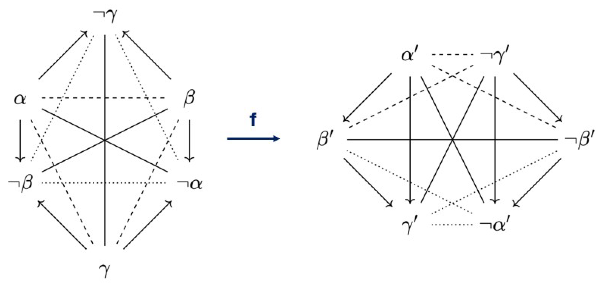
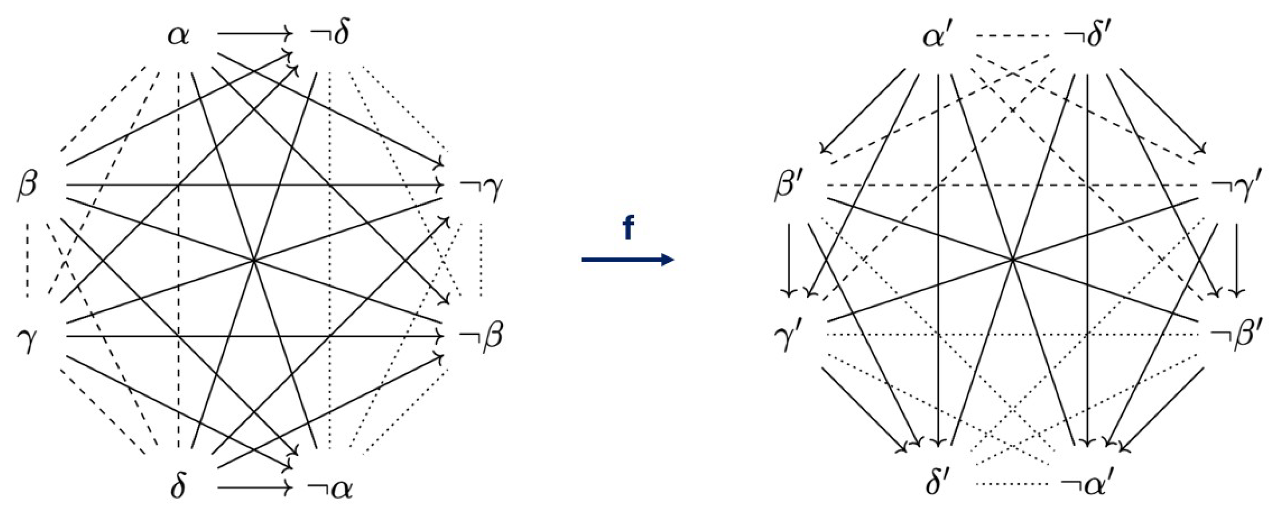
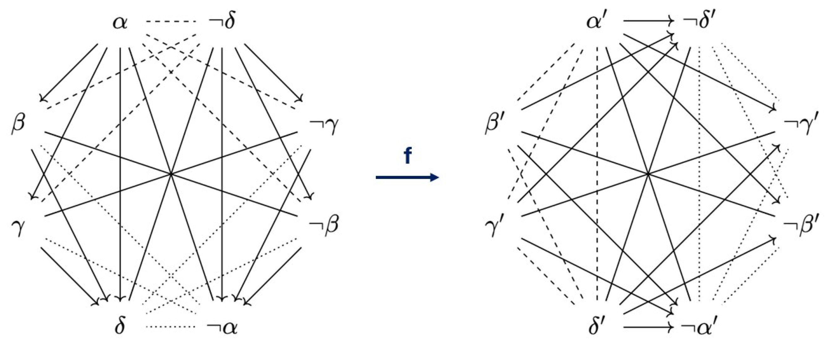
Example 9. 

Let us begin by considering a (generic) Moretti octagon D, as in the left of Figure 10, which is also known as an ${\alpha }_4$-structure. Let us also consider a (generic) Lenzen octagon $D^{\prime }$, as in the right of Figure 10, which is also known as a 4-ladder. From Corollaries 1 and 2, we already know that these individual diagrams, as well as their respective families, are $OI$-companions of each other. This means we can construct an $OI$-map f from D to $D^{\prime }$. For example, we can set

$$\begin{array}{cc}\hfill f\left(\alpha \right)& :={\alpha }^{\prime },\hfill \\ \hfill f(\neg \alpha )& :=\neg {\alpha }^{\prime },\hfill \\ \hfill f\left(\beta \right)& :={\beta }^{\prime },\hfill \\ \hfill f(\neg \beta )& :=\neg {\beta }^{\prime },\hfill \\ \hfill f\left(\gamma \right)& :={\gamma }^{\prime },\hfill \\ \hfill f(\neg \gamma )& :=\neg {\gamma }^{\prime }\hfill \\ \hfill f\left(\delta \right)& :={\delta }^{\prime },\hfill \\ \hfill f(\neg \delta )& :=\neg {\delta }^{\prime },\hfill \end{array}$$

getting our inspiration from Proposition 4 of [14]. This map f is visualized in Figure 10, from which it can be checked that it really is an $OI$-map. In this case, because there are 18 different Aristotelian families of octagons, it is more work (but still possible!) to prove that no other $OI$-companions of either D or $D^{\prime }$ exist. In other words, they are each other’s unique $OI$-companion. 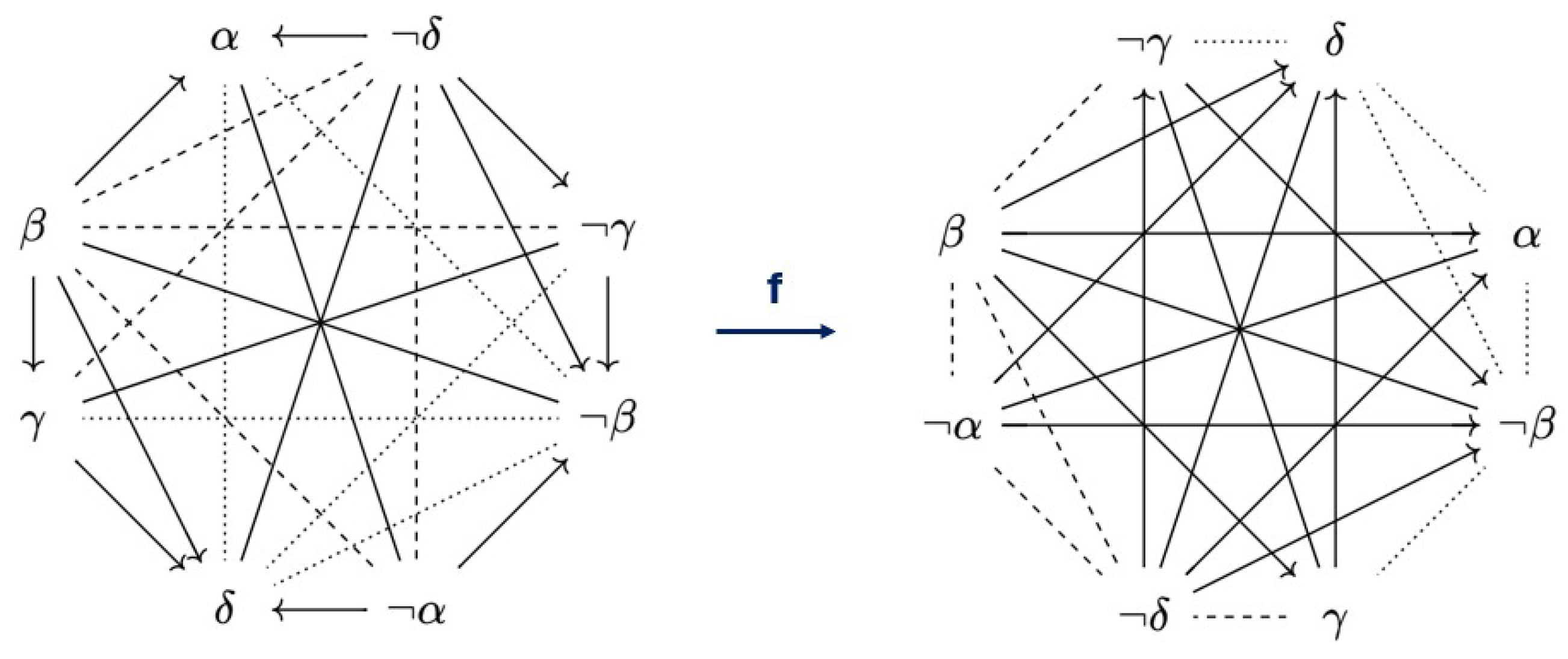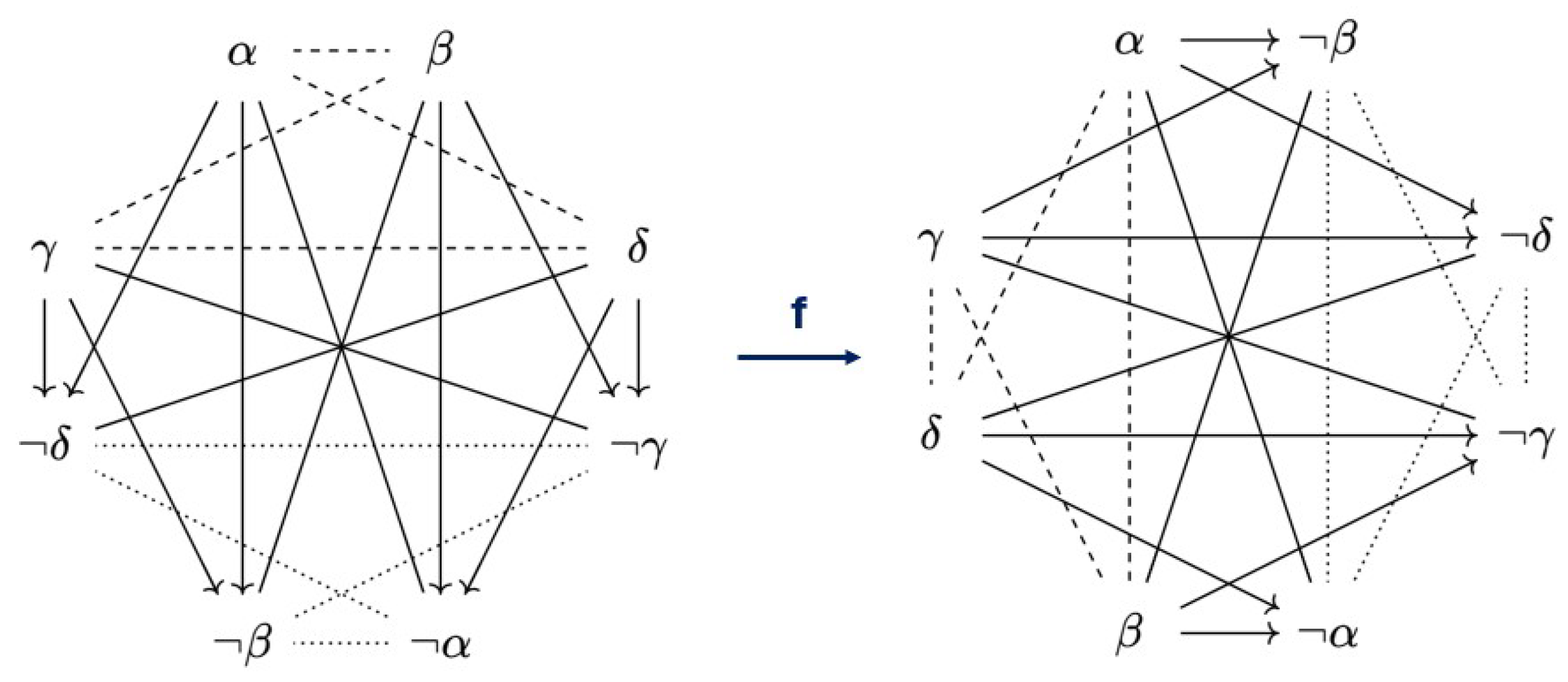The tedious proof of this fact, which we will not go over here, consists of checking the constellations of Aristotelian relations of all of the 17 other families, and showing that no $OI$-maps exist (analogous to Example 6).

Example 10. 

Let us now consider a (generic) Buridan octagon, as in the left of Figure 11. Interestingly enough, none of the octagons that have appeared before in the literature qualify as an $OI$-companion for D. This does not mean that Buridan octagons do not have $OI$-companions at all, but merely that if they exist, they are not well-known diagrams. To find an $OI$-companion for the Buridan octagons, we must find an octagon which has subalternations/(sub)contraries in every spot where the Buridan octagon has (sub)contraries/subalternations. Of course, there are multiple options to draw such a (generic) diagram, but most of those options are not consistent (e.g., because they would require putting a subalternation from α to β and from β to γ, but not one from α to γ), and thus do not give rise to an actual Aristotelian family. It turns out that there is in fact an $OI$-companion $D^{\prime }$ of D, which can be found in the right of Figure 11. Unlike the other Aristotelian families mentioned in this paper, the family of $D^{\prime }$ has hitherto not been studied in the literature. For a concrete example, which also establishes the consistency of this configuration of Aristotelian relations, we can take ${\alpha }^{\prime }:=00001,{\beta }^{\prime }:=10100,{\gamma }^{\prime }:=01100,$ and ${\delta }^{\prime }:=00010$ in the Boolean algebra ${\{0,1\}}^5$. To prove that it really is an $OI$-companion of D, let us define the $OI$-map f from $\mathcal{F}$ to ${\mathcal{F}}^{\prime }$ as

$$\begin{array}{cc}\hfill f\left(\alpha \right)& :={\alpha }^{\prime },\hfill \\ \hfill f(\neg \alpha )& :=\neg {\alpha }^{\prime },\hfill \\ \hfill f\left(\beta \right)& :={\beta }^{\prime },\hfill \\ \hfill f(\neg \beta )& :=\neg {\beta }^{\prime },\hfill \\ \hfill f\left(\gamma \right)& :={\gamma }^{\prime },\hfill \\ \hfill f(\neg \gamma )& :=\neg {\gamma }^{\prime },\hfill \\ \hfill f\left(\delta \right)& :={\delta }^{\prime },\hfill \\ \hfill f(\neg \delta )& :=\neg {\delta }^{\prime }.\hfill \end{array}$$

This map f is visualized in Figure 11, from which it can be checked that it really is an $OI$-map. It is possible to prove that this $OI$-companion of D is unique (up to Aristotelian isomorphism), and this can be done in the same (tedious) way as in the previous example.

Buridan octagons are often viewed, just like ladders, as having an implicative structure that is much more interesting than their oppositional structure. This is because a Buridan octagon always contains two SC hexagons (which are ladders), which can be seen in Figure 11 by removing the β-PCD and the γ-PCD, respectively [51]. Following this line of reasoning, the diagram on the right of Figure 11 can be viewed as having an oppositional structure that is much more interesting than its implicative structure.

Example 11. 

Let us consider a (generic) Béziau octagon D, as in Figure 12. We can construct an $OI$-map f from this diagram to itself. For example, we can set

$$\begin{array}{cc}\hfill f\left(\alpha \right)& :=\neg \gamma ,\hfill \\ \hfill f(\neg \alpha )& :=\gamma ,\hfill \\ \hfill f\left(\beta \right)& :=\beta ,\hfill \\ \hfill f(\neg \beta )& :=\neg \beta ,\hfill \\ \hfill f\left(\gamma \right)& :=\neg \alpha ,\hfill \\ \hfill f(\neg \gamma )& :=\alpha \hfill \\ \hfill f\left(\delta \right)& :=\neg \delta ,\hfill \\ \hfill f(\neg \delta )& :=\delta .\hfill \end{array}$$

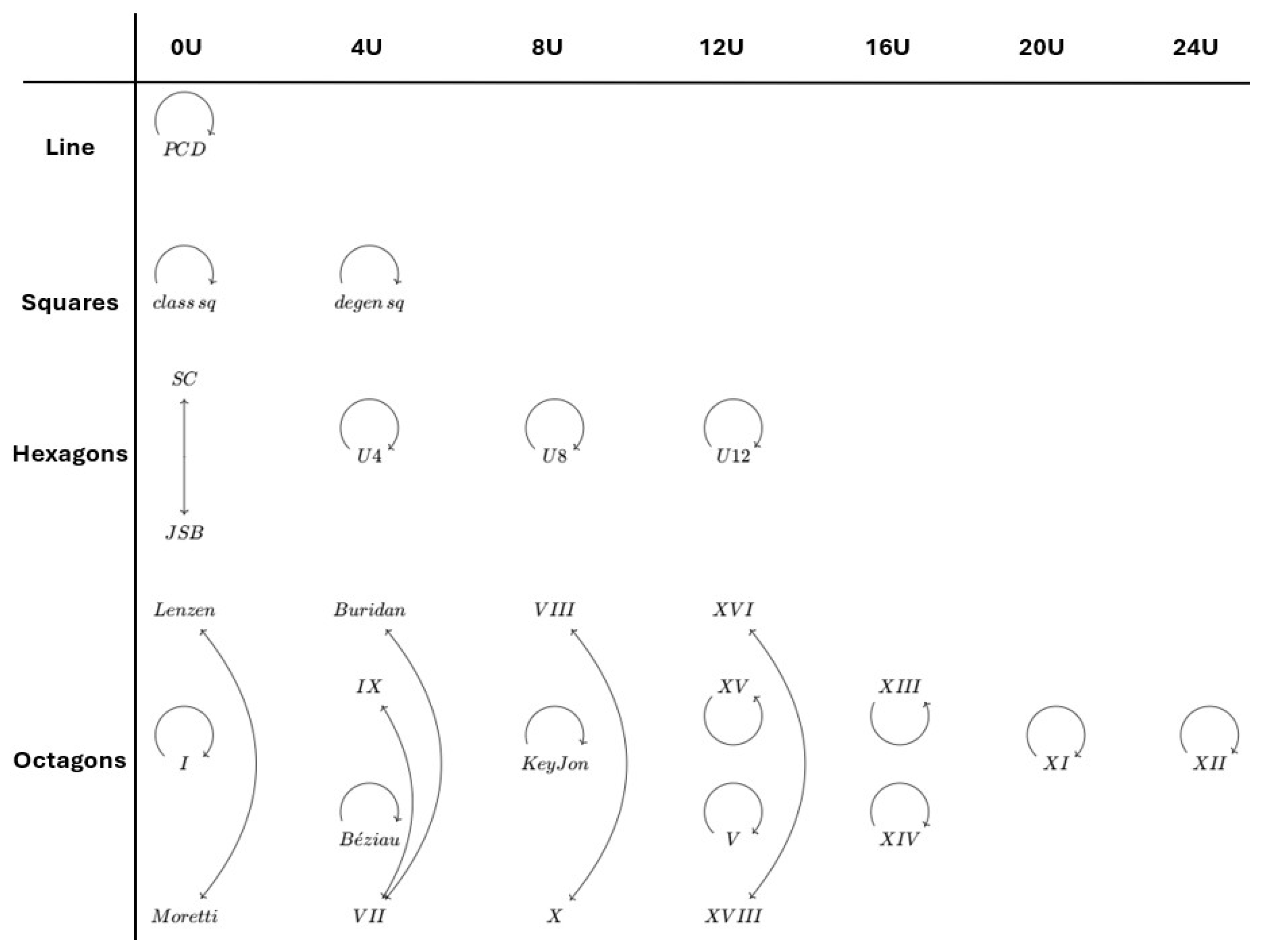
This map f is visualized in Figure 12, from which it can be checked that it really is an $OI$-map. Therefore, D is its own $OI$-companion. Because of Corollary 3, we can now say that the family of Béziau octagons is its own $OI$-companion. We could again use the same method (checking by hand all 17 other families of octagons) to prove that this $OI$-companion of D is unique up to Aristotelian isomorphism.

Example 12. 

Finally, let us consider a (generic) Keynes–Johnson octagon D, as in Figure 13. Similarly to a multitude of previous examples, we can construct an $OI$-map f from this diagram to itself. For example, we can set

$$\begin{array}{cc}\hfill f\left(\alpha \right)& :=\alpha ,\hfill \\ \hfill f(\neg \alpha )& :=\neg \alpha ,\hfill \\ \hfill f\left(\beta \right)& :=\neg \beta ,\hfill \\ \hfill f(\neg \beta )& :=\beta ,\hfill \\ \hfill f\left(\gamma \right)& :=\gamma ,\hfill \\ \hfill f(\neg \gamma )& :=\neg \gamma \hfill \\ \hfill f\left(\delta \right)& :=\neg \delta ,\hfill \\ \hfill f(\neg \delta )& :=\delta .\hfill \end{array}$$

This map f is visualized in Figure 13, from which it can be checked that it really is an $OI$-map. Therefore, D is its own $OI$-companion. Because of Corollary 3, we can now say that the family of Keynes–Johnson octagons is its own $OI$-companion. In this case, too, we can use the same method to prove that this $OI$-companion is unique up to Aristotelian isomorphism.

As was mentioned oftentimes before in this section, there are exactly 18 Aristotelian families of octagons. Even though we only covered five of them in detail in the series of Examples 9–12, we performed the computations for all 18 of them, which leads to the overview in Figure 14. In this overview, the arrows indicate which Aristotelian families are each other’s $OI$-companions, and the different Aristotelian families are ordered based on the size of their fragments (rows) and the number of occurrences of unconnectedness from Definition 3 (columns). Each of the families of octagons is labeled with a Roman numeral, except for the ones that have already received a more descriptive name in the literature (referring to the first known author to have used/studied a diagram of that family).

There are some interesting observations that can be made from the table in Figure 14. A major observation is that certain patterns start to emerge. On the one hand, the ${\alpha }_n$-structures and n-ladders form a pair of $OI$-companions in the first column, for every $n\in {\mathbb{N}}_0$. Since these two families do not coincide for $n>2$, this gives us a series of non-trivial pairs all the way down the table, starting from the hexagons. On the other hand, for each row, there is always exactly one Aristotelian family with the maximum number of occurrences of unconnectedness, which is located on the far right of the row. Analogously to Examples 5 and 8, such a diagram will always be an $OI$-companion of itself. Therefore, on the diagonal of the table, we have a series of families that are their own $OI$-companion. Additionally, starting from the second row, we always have exactly one Aristotelian family that consists of a single square of opposition together with only unconnectedness, which is located at the second rightmost spot of the row. Analogously to Examples 4 and 7 (the U8 hexagon), such a diagram will always be an $OI$-companion of itself. Therefore, we have another series of families that are their own $OI$-companion, which is located just left of/below the diagonal.

Aside from these patterns, there are some other things that are worthwhile mentioning. Firstly, it seems that there are more non-trivial instances of $OI$-companionship the more one goes downwards and leftwards in the table. This should not come as a surprise, since both of these directions allow for more Aristotelian relations to appear, which leads to a larger degree of complexity in the Aristotelian constellations, and thus leaves more room for asymmetry. Secondly, a recurring phrase throughout all of the examples in this section was that the $OI$-companion under consideration is unique up to Aristotelian isomorphism. However, looking at the octagon that is labeled with Roman numeral VII, we find that this is not true in general. In other words, $OI$-companionship is not functional. Additionally, up until this point, it still seems like each family has at least one $OI$-companion (i.e., $OI$-companionship is serial), but this, too, turns out to be false in general. We take a closer look at these final two remarks in the next section.

5. What OI-Companionship Is Not

In the previous sections, we defined the notion of $OI$-companionship, and studied this notion in a positive way. More concretely, Propositions 2 and 3 teach us that $OI$-companionship is a symmetric relation that functions both on the level of individual Aristotelian diagrams and on the level of entire Aristotelian families.

However, when we ask ourselves a question of the form “Does $OI$-companionship satisfy property X?”, the answer will not always be affirmative. For all important properties X that a relation might satisfy, it is important to know the answer to this question, even if it is a negative one. In this section, we will explain what $OI$-companionship is not. In other words, we go over some properties X that $OI$-companionship does not satisfy. More concretely, this relation is neither (ir)reflexive, nor transitive, nor functional, nor serial. The first two of these can be proven using the examples we already have at hand.

Proposition 4. 

$OI$-companionship is neither reflexive nor irreflexive.

Proof. 

Recall the generic JSB hexagon D from Example 6. In this example, we mentioned that D is not an $OI$-companion of itself, because its fragment contains a subset of three pairwise contrary elements, but not a subset of three pairwise subalternated elements. More concretely, suppose an $OI$-map f from D to itself would exist. Then, $f\left(\alpha \right),f\left(\beta \right)$, and $f\left(\gamma \right)$ should form a subset of three pairwise subalternated elements in D. It is immediately clear from Figure 6 that no such subset exists. Therefore, $OI$-companionship is not a reflexive relation.

Now, recall any of the Examples 3–5, 7, 8, 11, or 12. All of the Aristotelian diagrams/families occurring in these examples are $OI$-companions of themselves, which means that $OI$-companionship is not an irreflexive relation. □

Proposition 5. 

$OI$-companionship is not transitive.

Proof. 

Recall the JSB hexagon D and the SC hexagon $D^{\prime }$ from Example 6. By Proposition 1, D and $D^{\prime }$ are $OI$-companions. Because of symmetry (Proposition 2), $D^{\prime }$ and D are also $OI$-companions. If $OI$-companionship were a transitive relation, that would imply that D would be an $OI$-companion of itself, which we know is not the case from the proof of Proposition 4. □

Let us now move over to functionality and seriality, which are two other important properties that a relation might satisfy. For pedagogical reasons, we briefly state what we mean by these properties.

Definition 11. 

Let $X,Y$ be classes and let $R\subseteq X\times Y$ be a relation between X and Y. Then, R is called

• functional if, for every $x\in X$, there is exactly one $y\in Y$ such that $(x,y)\in R$,
• serial if, for every $x\in X$, there is at least one $y\in Y$ such that $(x,y)\in R$.

It is immediately clear from the above definition that functionality is a stronger property than seriality. Additionally, we need to be precise which classes $X,Y$ and which relation R we are considering. Let us start with the case in which $X=Y$ is the class of all Aristotelian diagrams and R is the relation of $OI$-companionship between Aristotelian diagrams (Definition 9). Because of Proposition 3, it is clear that we can never hope for functionality of this relation. Therefore, the case in which $X=Y$ is the class of all Aristotelian families, and R is the relation of $OI$-companionship between Aristotelian families (Definition 10), is much more interesting. However, it turns out that this relation is not functional either, as we briefly mentioned in the previous section while considering the octagon with Roman numeral label VII in the table of Figure 14. We now prove this in more detail by looking at a concrete counterexample.

Proposition 6. 

A single Aristotelian family can have more than one $OI$-companion. Therefore, $OI$-companionship between Aristotelian families is not functional.

Proof. 

Let us consider the following three fragments in bitstring algebras

$$\begin{array}{cc}\hfill {\mathcal{F}}_1& :=\{0010,0001,1001,0101,1101,1110,0110,1010\},\hfill \\ \hfill {\mathcal{F}}_2& :=\{00001,11101,10011,01011,11110,00010,01100,10100\},\hfill \\ \hfill {\mathcal{F}}_3& :=\{00001,11100,10100,01100,11110,00011,01011,10011\}.\hfill \end{array}$$

The fragment ${\mathcal{F}}_1$ resides in ${\{0,1\}}^4$, and the Aristotelian family ${\mathcal{D}}_1$ of the diagram $({\mathcal{F}}_1,{\{0,1\}}^4)$ is the family of Buridan octagons, which has been studied before in logical geometry [52]. In Example 10, we found its $OI$-companion $({\mathcal{F}}^{\prime },{\{0,1\}}^5)=({\mathcal{F}}_2,{\{0,1\}}^5)$, whose Aristotelian family ${\mathcal{D}}_2$ has not yet been studied before in the literature. Finally, the Aristotelian family ${\mathcal{D}}_3$ of the diagram $({\mathcal{F}}_3,{\{0,1\}}^5)$ has not yet appeared in the literature either. All of these Aristotelian diagrams are visualized in Figure 15, from which it is immediately clear that they belong to three distinct Aristotelian families. The diagrams in Figure 15 are visualized in a specific way that makes it easy to see how both $({\mathcal{F}}_1,{\{0,1\}}^4)$ and $({\mathcal{F}}_3,{\{0,1\}}^5)$ are $OI$-companions of $({\mathcal{F}}_2,{\{0,1\}}^5)$. Indeed, the concrete $OI$-maps $f_1:{\mathcal{F}}_1\to {\mathcal{F}}_2$ and $f_3:{\mathcal{F}}_3\to {\mathcal{F}}_2$ that do the job are given by

$$\begin{array}{cc}\hfill f_1\left(0010\right)=f_3\left(00001\right)& :=00001\hfill \\ \hfill f_1\left(0001\right)=f_3\left(11100\right)& :=11101\hfill \\ \hfill f_1\left(1001\right)=f_3\left(10100\right)& :=10011\hfill \\ \hfill f_1\left(0101\right)=f_3\left(01100\right)& :=01011\hfill \\ \hfill f_1\left(1101\right)=f_3\left(11110\right)& :=11110\hfill \\ \hfill f_1\left(1110\right)=f_3\left(00011\right)& :=00010\hfill \\ \hfill f_1\left(0110\right)=f_3\left(01011\right)& :=01100\hfill \\ \hfill f_1\left(1010\right)=f_3\left(10011\right)& :=10100.\hfill \end{array}$$

Therefore, ${\mathcal{D}}_2$ has both ${\mathcal{D}}_1$ and ${\mathcal{D}}_3$ as $OI$-companions. □

Proposition 6 tells us that it is not possible, for every Aristotelian family $\mathcal{D}$, to speak about the $OI$-companion of $\mathcal{D}$, because it can have more than one $OI$-companion. However, we can still hope that it is at least possible to speak about an $OI$-companion of $\mathcal{D}$, for any $\mathcal{D}$. In other words, we can ask ourselves the question whether $OI$-companionship (between Aristotelian families) is serial. However, it turns out that this question, too, has a negative answer. Since all $\sigma$-diagrams up to the octagons do have at least one $OI$-companion (see Figure 14), we need a completely different Aristotelian diagram to prove this, which is why the proof of Proposition 7 below uses a much larger diagram, which is, however, well-studied in logical geometry (usually under the geometric label of ‘rhombic dodecahedron’ or ‘RDH’) [49,53].

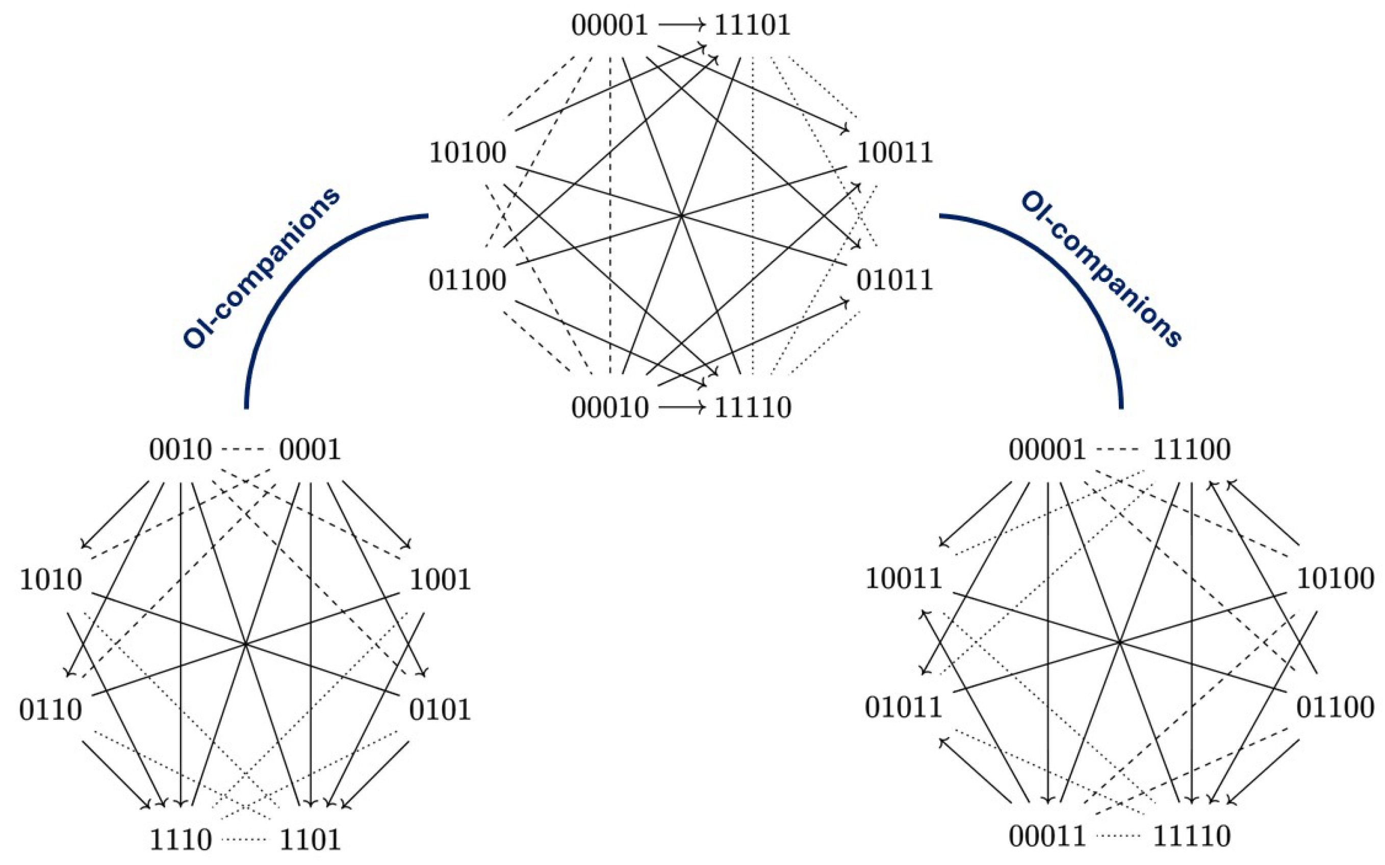
Note that we could make it very easy for ourselves, and we could simply use any Aristotelian diagram $(\mathcal{F},B)$ for which either 0 or 1 is inside the fragment $\mathcal{F}$. Indeed, we have that $BI(0,0)$ and $C(0,0)$, which means that after the application of an $OI$-map f, we would have that $BI\left(f\right(0),f(0\left)\right)$ and $LI\left(f\right(0),f(0\left)\right)$ (or $RI\left(f\right(0),f(0\left)\right)$) simultaneously, which is impossible. A similar reasoning holds true for 1. Therefore, any Aristotelian diagram that includes a top or bottom element has no $OI$-companion. However, a good number of researchers do not consider such diagrams to be genuine Aristotelian diagrams. Therefore, in the proof of Proposition 7 below, we use a diagram that does not contain a top or bottom element.

Proposition 7. 

A single Aristotelian diagram/family can possibly have zero $OI$-companions. Therefore, $OI$-companionship is not serial.

Proof. 

We will show that the Aristotelian diagram

$$D=(\mathcal{F},B):=({\{0,1\}}^4-\{0000,1111\},{\{0,1\}}^4)$$

has no $OI$-companion, which by Proposition 3 is enough to show that its Aristotelian family does not have an $OI$-companion either. Suppose, towards a contradiction, that D has an $OI$-companion $D^{\prime }=({\mathcal{F}}^{\prime },B^{\prime })$, and that $f:\mathcal{F}\to {\mathcal{F}}^{\prime }$ is an $OI$-map from D to $D^{\prime }$. The fragment $\mathcal{F}$ has a subset of four pairwise contrary elements, namely, $\{1000,0100,0010,0001\}$. These contrariety relations must turn into pairwise subalternations after the application of f, and thus $(\{f\left(1000\right),f\left(0100\right),f\left(0010\right),f\left(0001\right)\},{\le }_{B^{\prime }})$ must be a total order. Because of the symmetry of the fragment $\mathcal{F}$, we can assume, without loss of generality, that this total order is given by

$$f\left(1000\right)\le f\left(0100\right)\le f\left(0010\right)\le f\left(0001\right).$$

Now, 0100 and 1010 are contrary to each other in B, and therefore, we must have that $LI\left(f\right(0100),f(1010\left)\right)$ or $RI\left(f\right(0100),f(1010\left)\right)$. In the former case, we have that $f\left(1000\right)\le f\left(0100\right)\le f\left(1010\right),$ and thus $LI\left(f\right(1000),f(1010\left)\right)$ by transitivity of the order relation. However, 1000 and 1010 are not (sub)contrary to each other in B, so this contradicts the assumption that f is an $OI$-map. In the latter case, we have that $f\left(1010\right)\le f\left(0100\right)\le f\left(0010\right),$ and thus $LI\left(f\right(1010),f(0010\left)\right)$ by transitivity of the order relation. However, 1010 and 0010 are not (sub)contrary to each other in B, so this also contradicts the assumption that f is an $OI$-map. □

The results from this section seem to suggest that the relation of $OI$-companionship is quite complex, and behaves in intricate ways. Indeed, while it has two simple and intuitive properties, namely, being symmetric (Proposition 2) and being able to operate on the level of Aristotelian families (Proposition 3), all other simple properties that we tested have failed. Especially interesting is that both functionality and seriality fail, which means that it is impossible to discuss the idea of the or even an $OI$-companion of an arbitrary Aristotelian family. Some families, like all of the examples from Section 4, will have a unique $OI$-companion, while others will have more than that or none at all. This shows that the duality that exists between $\alpha$-structures and ladders, which was first discovered in [14], does not extend to the entire class of all Aristotelian families.

6. Conclusions

Aiming at a generalization of the duality between $\alpha$-structures and ladders, we created the notion of $OI$-companionship, which seems to capture its essence. Using this notion, we can formally capture Correia’s [4] idea that the square of opposition exhibits simultaneously a theory of negation and a theory of inference, by stating the square is its own $OI$-companion (cf. Example 4). While this notion has some useful intuitive properties, like being symmetric, and being able to operate on both the level of individual Aristotelian diagrams and entire Aristotelian families, it still behaves in unusual and intricate ways. More concretely, it is neither (ir)reflexive, nor transitive, nor functional, nor serial. This lack of seriality only appears when top/bottom elements are in play, and for some diagrams that have a large fragment.

Even with these unusual behaviors, from a general point of view, all of the particular squares, hexagons, and octagons that have appeared in the literature have a unique $OI$-companion up to Aristotelian isomorphism. Hence, even though the duality between $\alpha$-structures and ladders does not extend to all Aristotelian families through the notion of $OI$-companionship, it does apply to every important family that we know of. We have even found a family of octagons that has hitherto been neglected, which from now on can be viewed as the $OI$-companion of the well-known family of Buridan octagons. Our comprehensive treatment of $OI$-companionship thereby sheds new light on both well-studied and lesser-known Aristotelian families, and helps to shape the future direction of research in logical geometry. More concretely, a potential future research project could be to create an algorithm that, when given any Aristotelian diagram/family, produces the collection of all its $OI$-companions. Such a project could create a bridge from the theoretical results of this paper to the variety of applications of logical geometry.