
Convergence Analysis for System of Cayley Generalized Variational Inclusion on q-Uniformly Banach Space


Abstract
1. Introduction
2. Basic Concepts
- 1.
- Accretive, if for all , the following inequality holds:
- 2.
- Strictly accretive, if for all ,with equality if and only if ;
- 3.
- Strongly accretive, if there exists a constant such that
- 4.
- Lipschitz continuous, if there exists a constant such that
- 5.
- Relaxed Lipschitz continuous, if there exists a constant such that
3. Problem and Its Fixed Point Formulations
4. Main Result
5. Algorithm and Convergence Result
| Algorithm 1: System of resolvent-based iterative method. |
For the initial points , we compute the following schemes: |
| Algorithm 2: Coupled resolvent-based iterative method. |
For , we compute , based on the following iterative schemes: |
6. Numerical Result
7. Convergences Graphs and Tables
8. Conclusions
Author Contributions
Funding
Institutional Review Board Statement
Data Availability Statement
Conflicts of Interest
References
- Ahmad, R.; Ali, I.; Rahaman, M.; Ishtyak, M.; Yao, J.C. Cayley inclusion problem with its corresponding generalized resolvent equation problem in uniformly smooth Banach spaces. Appl. Anal. 2022, 101, 1354–1368. [Google Scholar] [CrossRef]
- Irfan, S.S.; Ahmad, I.; Islam, M.; Khan, M.F.; Rahaman, M.H. Convergence Analysis of S-iteration Process of Generalized Nonlinear Variational Inclusion Problem. Commun. Appl. Nonlinear Anal. 2024, 32, 344–361. [Google Scholar]
- Peeyada, P.; Kitisak, P.; Cholamjiak, W.; Yambangwai, D. Two inertial projective Mann forward-backward algorithm for variational inclusion problems and application to stroke prediction. Carpathian J. Math. 2024, 40, 381–398. [Google Scholar] [CrossRef]
- Alakoya, T.O.; Uzor, V.A.; Mewomo, O.T. A new projection and contraction method for solving split monotone variational inclusion, pseudomonotone variational inequality, and common fixed point problems. Comput. Appl. Math. 2023, 42, 3. [Google Scholar] [CrossRef]
- Baillon, J.B.; Bruck, R.E.; Reich, S. On the asymptotic behaviour of nonexpansive mappings and semigroups in Banach spaces. Houst. J. Math. 1978, 4, 1–9. [Google Scholar]
- Liu, L.; Yao, J.C. Iterative methods for solving variational inequality problems with a double-hierarchical structure in Hilbert spaces. Optimization 2022, 72, 2433–2461. [Google Scholar] [CrossRef]
- Noor, M.A.; Noor, K.I.; Rassias, M.T. System of General Variational Inclusions. In Analysis, Geometry, Nonlinear Optimization and Applications; World Scientific Publishing: Singapore, 2023; pp. 641–657. Available online: https://www.worldscientific.com/worldscibooks/10.1142/13002?srsltid=AfmBOorhbfNgfZil7K3iJtQZZ_Kt3qkr26yM8ThZ3r_Xbx4B-ANjWtGG#t=aboutBook (accessed on 4 May 2025).
- Ahmad, R.; Ansari, Q.H. An iterative algorithm for generalized nonlinear variational inclusions. Appl. Math. Lett. 2023, 13, 23–26. [Google Scholar] [CrossRef]
- Moudafi, A. A duality algorithm for solving general variational inclusions. Adv. Model. Optim. 2011, 13, 213–220. [Google Scholar]
- Hassouni, A.; Moudafi, A. A perturbed algorithm for variational inclusions. J. Math. Anal. Appl. 2011, 185, 706–712. [Google Scholar] [CrossRef]
- Fang, Y.P.; Huang, N.J. H-accretive operators and resolvent operator technique for solving variational inclusions in Banach spaces. J. Math. Anal. Appl. 1994, 183, 706–712. [Google Scholar] [CrossRef]
- Rockafellar, R.T. Monotone operators and the proximal point algorithms. SIAM J. Control. Optim. 1976, 14, 877–898. [Google Scholar] [CrossRef]
- Fang, Y.P.; Huang, N.J.; Thompson, H.B. A new system of variational inclusions with (H, η)-monotone operators in Hilbert spaces. Comput. Math. Appl. 2004, 49, 365–374. [Google Scholar] [CrossRef]
- Tam, M.K. Algorithms based on unions of nonexpansive maps. Optim. Lett. 2018, 12, 1019–1027. [Google Scholar] [CrossRef]
- Combettes, P.L. Solving monotone inclusions via composition of nonexpansive averaged operators. Optimization 2004, 53, 475–504. [Google Scholar] [CrossRef]
- Ahmad, R.; Ishtyak, M.; Rajpoot, A.K.; Wang, Y. Solving System of Mixed Variational Inclusions Involving Generalized Cayley Operator and Generalized Yosida Approximation Operator with Error Terms in q-Uniformly Smooth Space. Mathematics 2022, 10, 4131. [Google Scholar] [CrossRef]
- Balooee, J.; Postolache, M.; Yao, Y. System of generalized nonlinear variational-like inclusions and fixed point problems: Graph convergence with an application. Rend. Circ. Mat. Palermo Ser. 2 2024, 73, 1343–1384. [Google Scholar] [CrossRef]
- Alansari, M.; Akram, M.; Dilashad, M. Iterative Algorithms for a Generalized System of Mixed Variational-Like Inclusion Problems and Altering Points Problem. Stat. Optim. Inf. Comput. 2020, 8, 549–564. [Google Scholar] [CrossRef]
- Noor, M.A.; Noor, K.I. General bivariational inclusions and iterative methods. Int. J. Nonlinear Anal. Appl. 2023, 14, 309–324. [Google Scholar]


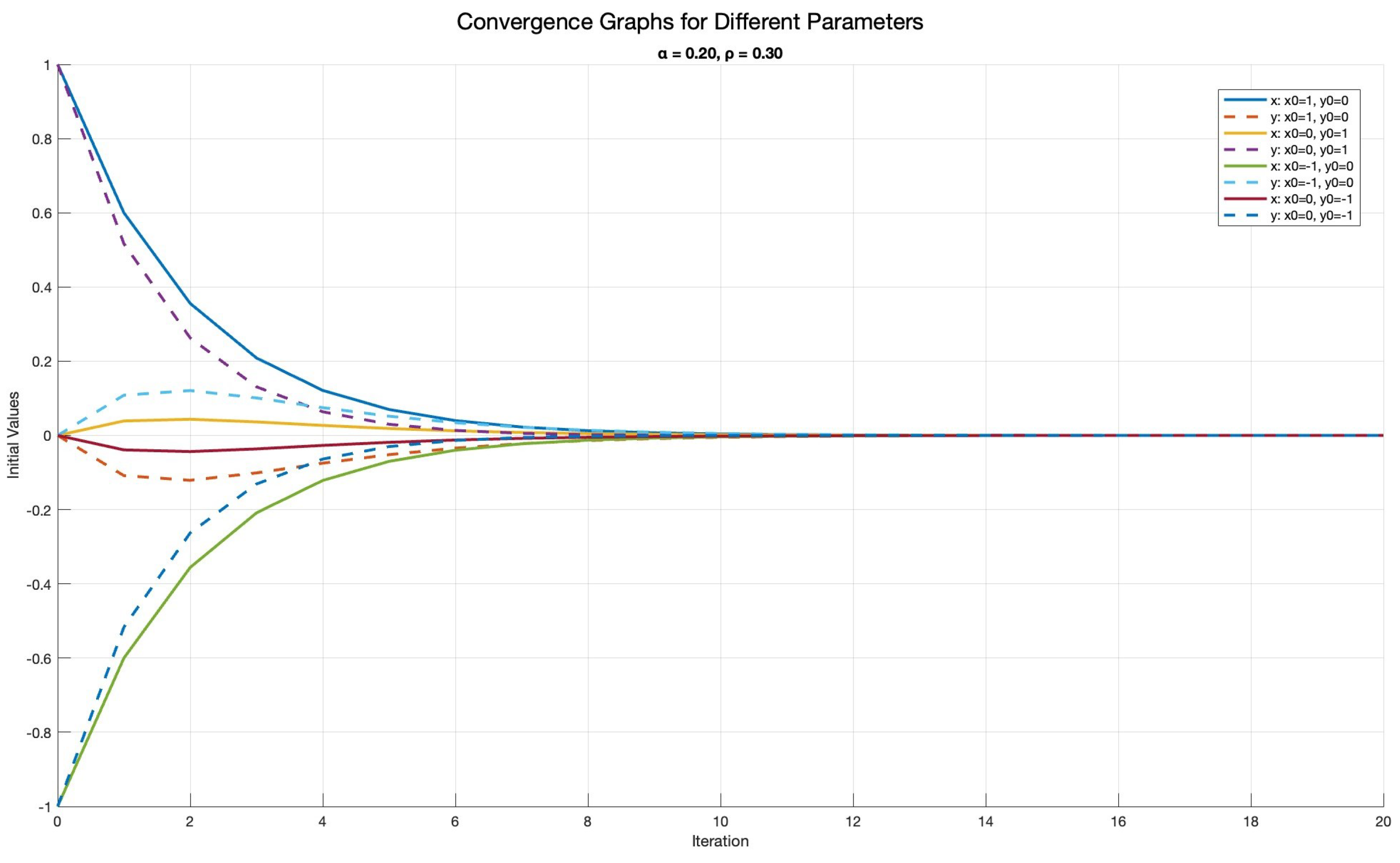
| Iteration | Initial | Initial | ||||
|---|---|---|---|---|---|---|
| 1 | 1 | 0 | 0.20 | 0.30 | 0.6000 | −0.1083 |
| 5 | 1 | 0 | 0.20 | 0.30 | 0.0699 | −0.0518 |
| 13 | 1 | 0 | 0.20 | 0.30 | 6.2912 | −0.0011 |
| 1 | 0 | 1 | 0.20 | 0.30 | 0.0390 | 0.5167 |
| 5 | 0 | 1 | 0.20 | 0.30 | 0.0186 | 0.0300 |
| 12 | 0 | 1 | 0.20 | 0.30 | 6.5987 | −2.4232 |
| 1 | −1 | 0 | 0.20 | 0.30 | −0.6000 | 0.1083 |
| 5 | −1 | 0 | 0.20 | 0.30 | −0.0699 | 0.0518 |
| 13 | −1 | 0 | 0.20 | 0.30 | −6.2912 | 0.0011 |
| 1 | 0 | −1 | 0.20 | 0.30 | −0.0390 | −0.5167 |
| 5 | 0 | −1 | 0.20 | 0.30 | −0.0186 | −0.0300 |
| 13 | 0 | −1 | 0.20 | 0.30 | −3.8647 | 1.9668 |
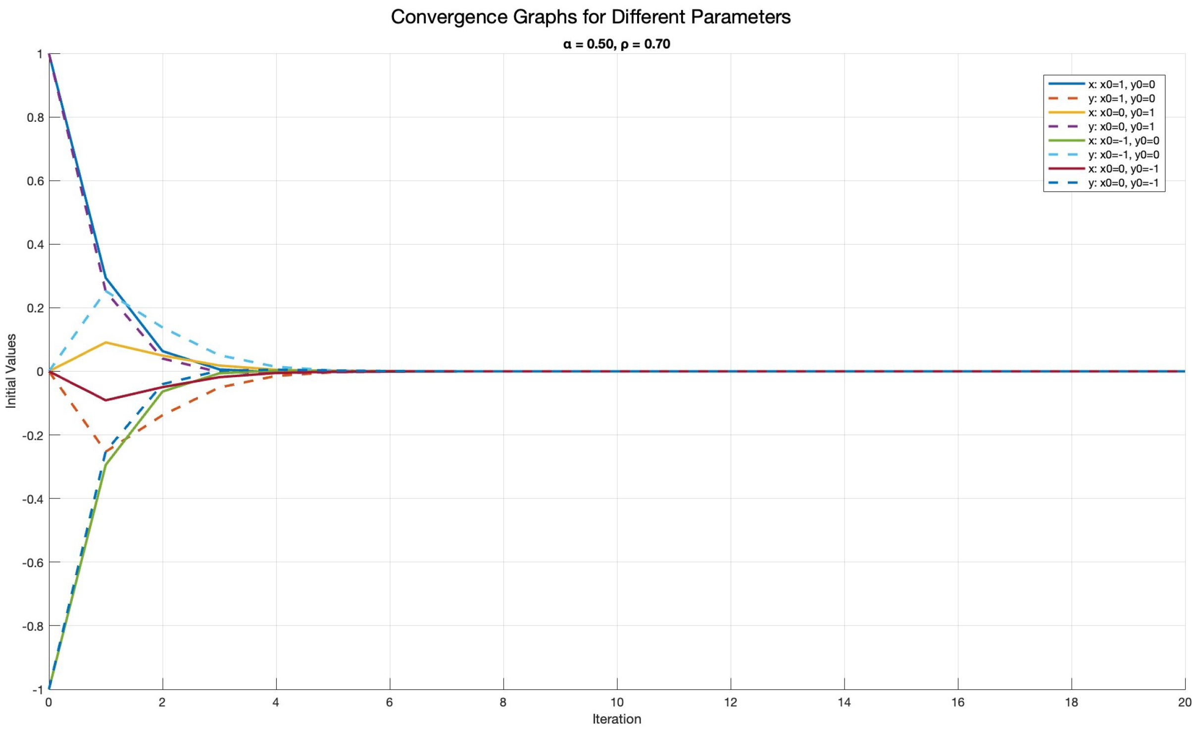
| Iteration | Initial | Initial | ||||
|---|---|---|---|---|---|---|
| 1 | 1 | 0 | 0.50 | 0.70 | 0.2942 | −0.2528 |
| 3 | 1 | 0 | 0.50 | 0.70 | 0.0061 | −0.0507 |
| 6 | 1 | 0 | 0.50 | 0.70 | −8.8867 | −1.8741 |
| 1 | 0 | 1 | 0.50 | 0.70 | 0.0910 | 0.2514 |
| 3 | 0 | 1 | 0.50 | 0.70 | 0.0183 | −0.0024 |
| 6 | 0 | 1 | 0.50 | 0.70 | 6.7466 | −9.2038 |
| 1 | −1 | 0 | 0.50 | 0.70 | −0.2942 | 0.2528 |
| 3 | −1 | 0 | 0.50 | 0.70 | −0.0061 | 0.0507 |
| 6 | −1 | 0 | 0.50 | 0.70 | 8.8867 | 1.8741 |
| 1 | 0 | −1 | 0.50 | 0.70 | −0.0910 | −0.2514 |
| 3 | 0 | −1 | 0.50 | 0.70 | −0.0183 | 0.0024 |
| 7 | 0 | −1 | 0.50 | 0.70 | 6.3908 | 2.4843 |
| Iteration | Initial | Initial | ||||
|---|---|---|---|---|---|---|
| 1 | 1 | 0 | 0.70 | 0.90 | 0.2875 | −0.3250 |
| 4 | 1 | 0 | 0.70 | 0.90 | −0.0141 | −0.0292 |
| 8 | 1 | 0 | 0.70 | 0.90 | −1.0794 | 6.2448 |
| 1 | 0 | 1 | 0.70 | 0.90 | 0.1170 | 0.3625 |
| 4 | 0 | 1 | 0.70 | 0.90 | 0.0105 | −0.0073 |
| 8 | 0 | 1 | 0.70 | 0.90 | −2.2481 | −2.5205 |
| 1 | −1 | 0 | 0.70 | 0.90 | −0.2875 | 0.3250 |
| 4 | −1 | 0 | 0.70 | 0.90 | 0.0141 | 0.0292 |
| 7 | −1 | 0 | 0.70 | 0.90 | 7.8873 | −0.0010 |
| 1 | 0 | −1 | 0.70 | 0.90 | −0.1170 | −0.3625 |
| 4 | 0 | −1 | 0.70 | 0.90 | −0.0105 | 0.0073 |
| 7 | 0 | −1 | 0.70 | 0.90 | 3.6560 | 0.0010 |
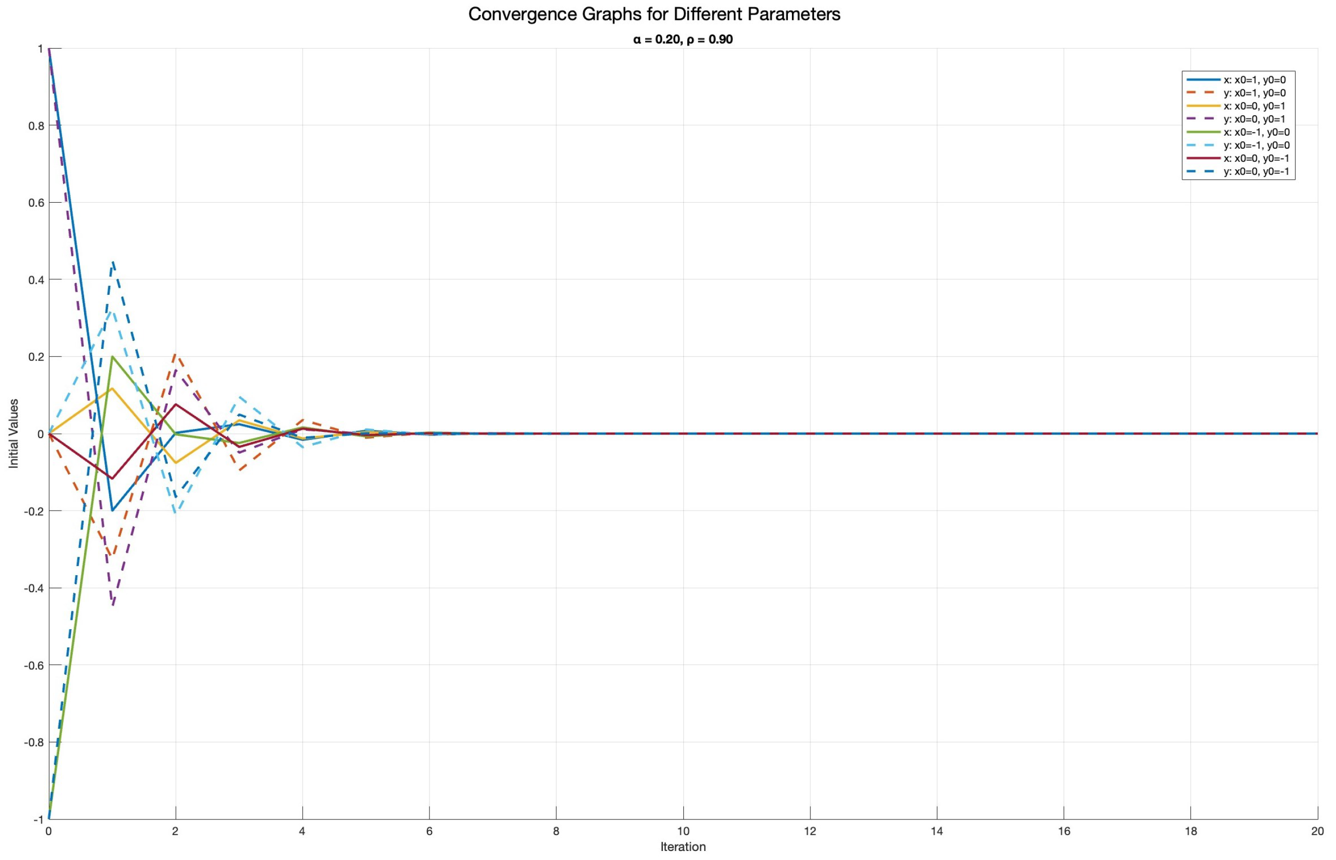
| Iteration | Initial | Initial | ||||
|---|---|---|---|---|---|---|
| 1 | 1 | 0 | 0.20 | 0.90 | −0.2000 | −0.3250 |
| 4 | 1 | 0 | 0.20 | 0.90 | −0.0161 | 0.0352 |
| 7 | 1 | 0 | 0.20 | 0.90 | 8.2084 | −1.9626 |
| 1 | 0 | 1 | 0.20 | 0.90 | 0.1170 | −0.4500 |
| 4 | 0 | 1 | 0.20 | 0.90 | −0.0127 | 0.0110 |
| 6 | 0 | 1 | 0.20 | 0.90 | −8.6052 | −8.6711 |
| 1 | −1 | 0 | 0.20 | 0.90 | 0.2000 | 0.3250 |
| 4 | −1 | 0 | 0.20 | 0.90 | 0.0161 | −0.0352 |
| 7 | −1 | 0 | 0.20 | 0.90 | −8.2084 | 1.9626 |
| 1 | 0 | −1 | 0.20 | 0.90 | −0.1170 | 0.4500 |
| 4 | 0 | −1 | 0.20 | 0.90 | 0.0127 | −0.0110 |
| 6 | 0 | −1 | 0.20 | 0.90 | 8.6052 | 8.6711 |
Disclaimer/Publisher’s Note: The statements, opinions and data contained in all publications are solely those of the individual author(s) and contributor(s) and not of MDPI and/or the editor(s). MDPI and/or the editor(s) disclaim responsibility for any injury to people or property resulting from any ideas, methods, instructions or products referred to in the content. |
© 2025 by the authors. Licensee MDPI, Basel, Switzerland. This article is an open access article distributed under the terms and conditions of the Creative Commons Attribution (CC BY) license (https://creativecommons.org/licenses/by/4.0/).
Share and Cite
Khan, M.F.; Irfan, S.S.; Ahmad, I. Convergence Analysis for System of Cayley Generalized Variational Inclusion on q-Uniformly Banach Space. Axioms 2025, 14, 361. https://doi.org/10.3390/axioms14050361
Khan MF, Irfan SS, Ahmad I. Convergence Analysis for System of Cayley Generalized Variational Inclusion on q-Uniformly Banach Space. Axioms. 2025; 14(5):361. https://doi.org/10.3390/axioms14050361
Chicago/Turabian StyleKhan, Mohd Falahat, Syed Shakaib Irfan, and Iqbal Ahmad. 2025. "Convergence Analysis for System of Cayley Generalized Variational Inclusion on q-Uniformly Banach Space" Axioms 14, no. 5: 361. https://doi.org/10.3390/axioms14050361
APA StyleKhan, M. F., Irfan, S. S., & Ahmad, I. (2025). Convergence Analysis for System of Cayley Generalized Variational Inclusion on q-Uniformly Banach Space. Axioms, 14(5), 361. https://doi.org/10.3390/axioms14050361