Finite Volume Method and Its Applications in Computational Fluid Dynamics

Abstract

Various numerical techniques have been developed to address multiple problems in computational fluid dynamics (CFD). The finite volume method (FVM) is a numerical technique used for solving partial differential equations that represent conservation laws by dividing the domain into control volumes and ensuring flux balance at their boundaries. Its conservative characteristics and capability to work with both structured and unstructured grids make it suitable for addressing issues related to fluid flow, heat transfer, and diffusion. This article introduces an FVM for the linear advection and nonlinear Burgers’ equations through a fifth-order targeted essentially non-oscillatory (TENO5) scheme. Numerical experiments showcase the precision and effectiveness of TENO5, emphasizing its benefits for computational fluid dynamics (CFD) simulations.

1. Introduction

Computational fluid dynamics (CFD) refers to the numerical analysis of systems involving fluid motion, heat transfer, and related phenomena, such as chemical reactions, through computer simulations. This computational approach is widely applied across both industrial and non-industrial sectors.

CFD techniques play a crucial role in various industries, such as the design, research, development, and production of aircraft and jet engines. Furthermore, CFD has found extensive application across an array of other industries, demonstrating its wide-ranging impact and utility [1,2].

The finite volume method (FVM) is a numerical technique developed to solve partial differential equations (PDEs) that encapsulate various conservation laws, including those related to mass, momentum, and energy. By integrating these equations over well-defined control volumes, the FVM effectively transforms them into a system of algebraic equations. This transformation is crucial as it inherently preserves local conservation properties, ensuring that fundamental physical principles are maintained. Over the years, the finite volume method has undergone significant evolution, adapting to tackle increasingly complex challenges within the field of computational fluid dynamics (CFD). Its versatility and robustness render it a recommended choice for simulating fluid flow across a wide range of applications, from aerospace engineering to environmental modeling [1,2,3,4].

The FVM framework includes several essential computational steps. Initially, a mesh is generated to partition the computational domain into small, discrete control volumes that can be analyzed independently. Next, the evaluation of flux across the boundaries of these control volumes is performed, which involves calculating conserved quantities such as fluid velocity and pressure. Finally, appropriate boundary conditions are applied to define the behavior of the fluid at the edges of the computational domain. By carefully following these steps, the finite volume method provides an effective and reliable framework for simulating complex phenomena in fluid dynamics [1,2,3].

There have been several studies using numerical methods presented in the literature for solving nonlinear partial differential equations (PDEs). Recent studies have been proposed based on physics-informed neural networks (PINNs) and finite difference methods (FDMs), and they have shown promising performances for modeling complex waves and nonlinear dynamics, such as Burgers’ and sine-Gordon equations [5,6]. Although these techniques provide valuable insights, this work chooses the finite volume method (FVM) framework due to its conservative implementation and robustness concerning sharp gradients and discontinuities, which are important when dealing with high-resolution schemes like TENO5.

The finite volume method (FVM) has been applied by researchers to address a variety of problems in computational fluid dynamics. The FVM is effective in solving the Poisson equation, heat equation, and diffusion equation, which govern numerous physical processes [7,8]. Additionally, its application with unstructured moving meshes for simulations highlights its capability to manage free surface flows [9].

In the finite volume method (FVM), various numerical schemes have unique characteristics, such as conservativeness, boundedness, and transportiveness. This research utilizes a high-order method, specifically the fifth-order targeted essentially non-oscillatory (TENO5) scheme, which aims to improve both numerical stability and accuracy.

The primary aim of this paper is to explore the fifth-order targeted essentially non-oscillatory (TENO5) scheme within the finite volume method for addressing a one-dimensional linear advection equation and a two-dimensional nonlinear Burgers’ equation that includes diffusion. The finite volume method will be developed and utilized to tackle these equations, and numerical experiments will be conducted to evaluate the approximate solutions against the exact solutions.

This paper is organized as follows: Section 2 provides a brief overview of the targeted essentially non-oscillatory (TENO) scheme. Section 3 presents numerical experiments to evaluate the performance of the TENO scheme. Section 4 includes a discussion of the results. Finally, Section 5 concludes the paper and proposes future research directions, particularly focusing on extending the higher-order capabilities of the TENO scheme and exploring its application in 3D numerical experiments.

2. Targeted Essentially Non-Oscillatory (TENO) Scheme

The targeted essentially non-oscillatory (TENO) approach is crafted to minimize oscillations that may arise in the numerical solutions of problems featuring sharp gradients or discontinuities, commonly seen in computational fluid dynamics (CFD) and other areas that require the simulation of wave propagation or transport processes. TENO effectively addresses turbulence while maintaining controllable, low numerical dissipation. In the TENO approach, a scale separation technique adeptly distinguishes between discontinuities and minor fluctuations, leading to reduced dissipation when compared to conventional methods, which can produce oscillations and instabilities in the presence of strong shocks [10,11,12].

This paper will discuss the fifth-order version of the method, known as the fifth-order targeted essentially non-oscillatory (TENO5) scheme.

2.1. TENO Methodology in FVM Framework

The scalar hyperbolic conservation law in one dimension is given by

$${\displaystyle \frac{\partial u}{\partial t}}+{\displaystyle \frac{\partial f\left(u\right)}{\partial x}}=0.$$

(1)

An equivalent formulation is as follows:

$$u_t+f{\left(u\right)}_x=0.$$

(2)

The initial condition is defined as

$$u(x,0)=u_0\left(x\right).$$

(3)

Discretizing Equation (1) on uniform cell elements, e.g., $I_i=[x_{i-{\displaystyle \frac{1}{2}}},x_{i+{\displaystyle \frac{1}{2}}}]$ with $\mathrm{\Delta }x=x_{i+{\displaystyle \frac{1}{2}}}-x_{i-{\displaystyle \frac{1}{2}}}$ for $i=0,1,\dots ,N$, the system reduces to a set of ordinary differential equations (ODEs) of the form

$${\displaystyle \frac{d{\overline{u}}_i}{dt}}=-{\displaystyle \frac{1}{\mathrm{\Delta }x}}{\int }_{x_i-\mathrm{\Delta }x/2}^{x_i+\mathrm{\Delta }x/2}{\displaystyle \frac{\partial f}{\partial x}}dx,i=0,1,\dots ,N.$$

(4)

where

$${\overline{u}}_i\left(t\right)={\displaystyle \frac{1}{\mathrm{\Delta }x}}{\int }_{x_i-\mathrm{\Delta }x/2}^{x_i+\mathrm{\Delta }x/2}u(x,t)dx,$$

(5)

expresses the cell-averaged conservative variable in $I_i$.

Moreover, Equation (4) could be approximated as

$${\displaystyle \frac{d{\overline{u}}_i}{dt}}\approx -{\displaystyle \frac{1}{\mathrm{\Delta }x}}({\widehat{f}}_{i+{\displaystyle \frac{1}{2}}}-{\widehat{f}}_{i-{\displaystyle \frac{1}{2}}}),$$

(6)

The numerical fluxes at the cell interface ${\widehat{f}}_{i+{\displaystyle \frac{1}{2}}}$ and ${\widehat{f}}_{i-{\displaystyle \frac{1}{2}}}$ in the semi-discrete finite volume scheme, which is given in Equation (6), can be computed using a Riemann solver. For example, the flux ${\widehat{f}}_{i+{\displaystyle \frac{1}{2}}}$ is given by

$${\widehat{f}}_{i+{\displaystyle \frac{1}{2}}}=f_{i+{\displaystyle \frac{1}{2}}}^{\mathrm{Riemann}}(u_{i+{\displaystyle \frac{1}{2}}}^L,u_{i+{\displaystyle \frac{1}{2}}}^R).$$

(7)

Here, $u_{i+{\displaystyle \frac{1}{2}}}^L$ and $u_{i+{\displaystyle \frac{1}{2}}}^R$ represent left-biased reconstruction and right-biased reconstruction, respectively, within cell $I_i$.

Even though the exact Riemann problem can be solved at the cell interface, approximate Riemann solvers are commonly used for their high efficiency. There are many different variants of approximate Riemann solvers, such as the Rusanov flux, the Roe flux, and the HLLC flux, as detailed in [12,13]. They can be represented in a general form as follows:

$$f_{i+{\displaystyle \frac{1}{2}}}^{\mathrm{Riemann}}\left(u_{i+{\displaystyle \frac{1}{2}}}^L,u_{i+{\displaystyle \frac{1}{2}}}^R\right)=\underset{\mathrm{Non}-\mathrm{dissipative}\mathrm{central}\mathrm{flux}\mathrm{term}}{\underbrace{{\displaystyle \frac{1}{2}}\left[f\left(u_{i+{\displaystyle \frac{1}{2}}}^L\right)+f\left(u_{i+{\displaystyle \frac{1}{2}}}^R\right)\right]}}-\underset{\mathrm{Numerical}\mathrm{Dissipation}\mathrm{term}}{\underbrace{{\displaystyle \frac{1}{2}}\left|{\tilde{\partial }}_{i+{\displaystyle \frac{1}{2}}}\right|\left(u_{i+{\displaystyle \frac{1}{2}}}^R-u_{i+{\displaystyle \frac{1}{2}}}^L\right)}}.$$

(8)

where ${\tilde{\partial }}_{i+{\displaystyle \frac{1}{2}}}$ denotes the characteristic signal velocity evaluated at the cell interface.

The reconstruction candidate stencils: To achieve high-order reconstruction, a polynomial can be found for each candidate stencil by solving a linear system through Equation (5) with an approximation that is represented by

$$u_r\left(x\right)\approx {\widehat{u}}_r\left(x\right)=\sum _{l=0}^{k-1}{a}_{l,r}{x}^l.$$

(9)

where k indicates the stencil’s width. The coefficient $a_l$ is determined by solving the system of linear algebraic equations formed by substituting $u_r\left(x\right)$ into Equation (5) and evaluating the integral functions at the stencil nodes. In terms of the five-point scheme, the reconstructed conservative variable at the cell interface can be obtained as demonstrated in [10,11].

Scale separation: To separate smooth scales from discontinuities effectively, the smoothness indicators are defined as follows:

$${\gamma }_r={\left(C+{\displaystyle \frac{{\tau }_K}{{\beta }_{r,k}+\epsilon }}\right)}^q.r=0,\dots ,3.$$

(10)

where the parameters are $C=1,q=6$, and $\epsilon ={10}^{-40}$ to avoid a zero denominator, and K is the number of points.

${\beta }_{r,k}$ can be determined using

$${\beta }_{r,k}=\sum _{l=1}^{k-1}\mathrm{\Delta }{x}^{2l-1}{\int }_{x_{i-{\displaystyle \frac{1}{2}}}}^{x_{i+{\displaystyle \frac{1}{2}}}}{\left({\displaystyle \frac{d^l}{d{x}^l}}{\widehat{u}}_r\left(x\right)\right)}^{2}dx.$$

(11)

To obtain a high-order accurate scheme at the critical points, the global reference smoothness indicator $\tau$ is introduced for the five-point scheme, as presented in [11].

The TENO scheme is based on the principle of either abandoning the non-smooth stencil or applying the stencil with the optimal linear weights for the final reconstruction. To achieve this, the smoothness indicators are normalized as follows:

$${\chi }_r={\displaystyle \frac{{\gamma }_r}{{\sum }_{r=0}^3{\gamma }_r}}.$$

(12)

Here, the sharp cut-off function is defined by

$${\delta }_r=\left\{\begin{array}{cc}0,\hfill & \mathrm{if}{\chi }_r<C_T,\hfill \\ 1,\hfill & \mathrm{otherwise}.\hfill \end{array}\right.$$

(13)

The cut-off parameter $C_T$ determines the dissipation properties of the resulting scheme, and it is typically set to $C_T={10}^{-5}$.

If the large candidate stencil is judged to be smooth, i.e., ${\delta }_3=1$, the final reconstruction $u_{i+{\displaystyle \frac{1}{2}}}^L$ can be directly expressed as $u_{3,i+{\displaystyle \frac{1}{2}}}^L$. Otherwise, the final reconstruction is obtained through a nonlinear combination of the remaining small stencils, expressed as

$$u_{i+{\displaystyle \frac{1}{2}}}^L=\sum _{r=0}^2{w}_r{u}_{r,i+{\displaystyle \frac{1}{2}}}^L.$$

(14)

where the weight $w_r$ is expressed as

$$w_r={\displaystyle \frac{{\alpha }_r}{{\sum }_{r=0}^2{\alpha }_r}},{\alpha }_r=d_r{\delta }_r,r=0,1,2.$$

(15)

Here, $d_r$ is the optimal weight to achieve the maximum accuracy order with the full stencil [10,11,14].

2.2. Time Discretization for TENO Scheme

After employing the finite volume method (FVM) and discretizing the spatial derivatives using the TENO scheme, the semi-discrete form of the governing equation can be expressed as

$${\displaystyle \frac{du}{dt}}=L\left(u\right).$$

(16)

where $L\left(u\right)$ denotes the operator used for spatial discretization.

For time integration, a third-order strong-stability-preserving (SSP) Runge–Kutta method is utilized:

$$\begin{array}{cc}\hfill u^{\left(1\right)}& =u^{\left(n\right)}+\mathrm{\Delta }tL\left(u^{\left(n\right)}\right),\hfill \\ \hfill u^{\left(2\right)}& ={\displaystyle \frac{3}{4}}{u}^{\left(n\right)}+{\displaystyle \frac{1}{4}}{u}^{\left(1\right)}+{\displaystyle \frac{1}{4}}\mathrm{\Delta }tL\left(u^{\left(1\right)}\right),\hfill \\ \hfill u^{(n+1)}& ={\displaystyle \frac{1}{3}}{u}^{\left(n\right)}+{\displaystyle \frac{2}{3}}{u}^{\left(2\right)}+{\displaystyle \frac{2}{3}}\mathrm{\Delta }tL\left(u^{\left(2\right)}\right).\hfill \end{array}$$

(17)

This explicit Runge–Kutta method provides strong stability characteristics while achieving third-order temporal accuracy [10,11,12].

3. Numerical Experiments

In this section, two numerical experiments will be carried out to solve the linear advection of multiple waves and two-dimensional Burgers’ equation with diffusion for comparison purposes and to verify the results.

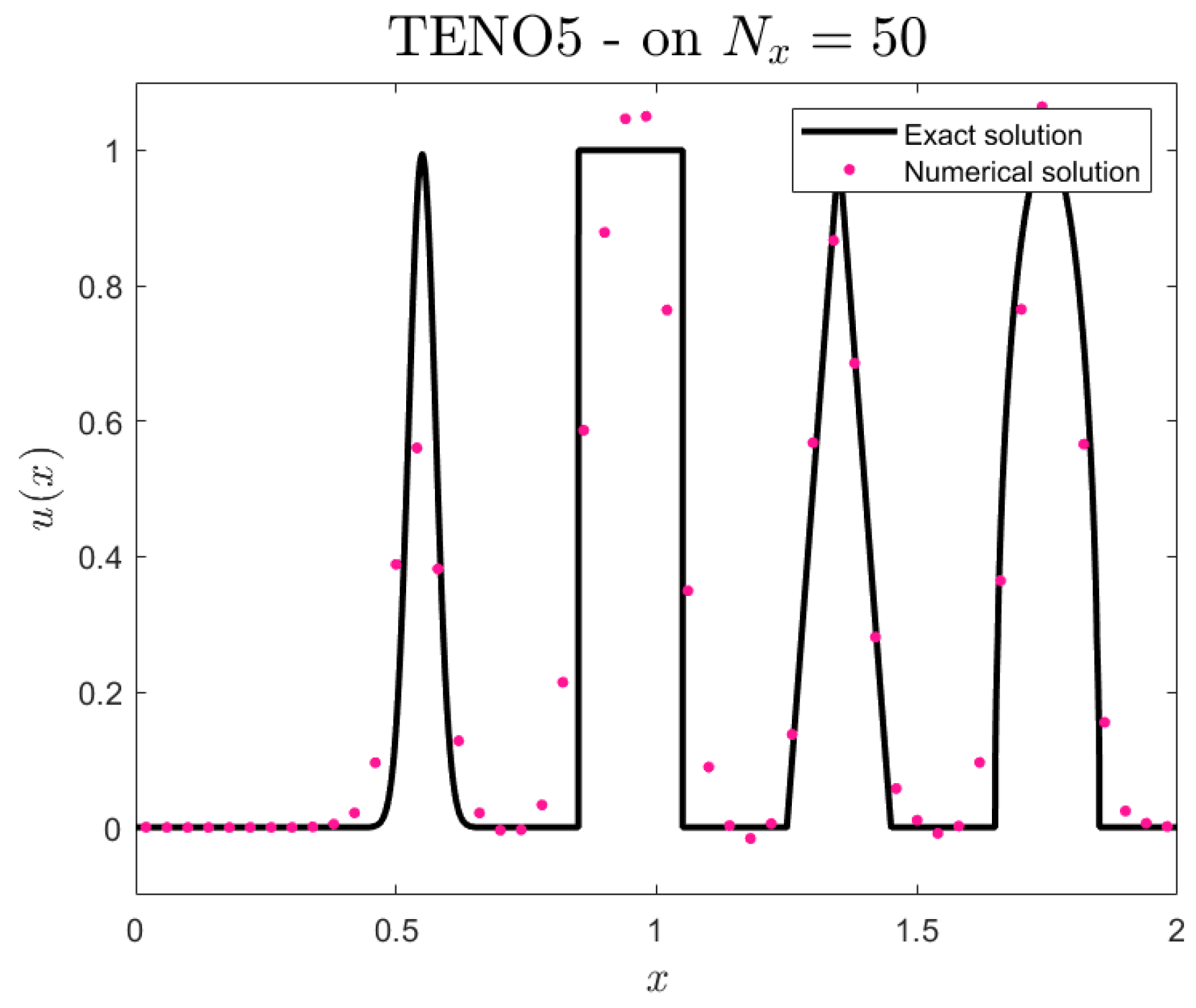
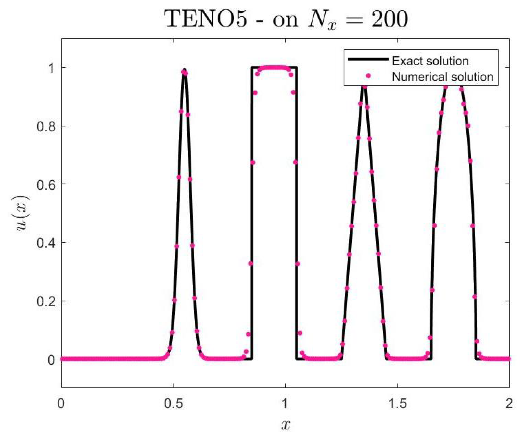
3.1. Linear Advection of Multiple Waves

Consider the one-dimensional linear advection equation

$${\displaystyle \frac{\partial u}{\partial t}}+{\displaystyle \frac{\partial u}{\partial x}}=0.$$

(18)

with the initial condition

$$u(x,0)=\left\{\begin{array}{cc}{\displaystyle \frac{1}{6}}[G(x-1,\beta ,z-\theta )+G(x-1,\beta ,z+\theta )+4G(x-1,\beta ,z)],\hfill & \mathrm{if}0.2\le x<0.4,\\ 1,\hfill & \mathrm{if}0.6\le x\le 0.8,\\ 1-\left|10\right(x-1.1\left)\right|,\hfill & \mathrm{if}1.0\le x\le 1.2,\\ {\displaystyle \frac{1}{6}}[F(x-1,\alpha ,a-\theta )+F(x-1,\alpha ,a+\theta )+4F(x-1,\alpha ,a)],\hfill & \mathrm{if}1.4\le x<1.6,\\ 0,\hfill & \mathrm{otherwise}.\end{array}\right.$$

(19)

where

$$G(x,\beta ,z)=e^{-\beta {(x-z)}^2},F(x,\alpha ,a)=\sqrt{max\left(1-{\alpha }^2{(x-a)}^2,0\right)}.$$

(20)

The parameters are given as

$$a=0.5,z=-0.7,\theta =0.005,\alpha =10,\beta ={\displaystyle \frac{log\left(2\right)}{36{\theta }^2}}.$$

(21)

The initial condition consists of a Gaussian pulse, a square wave, a sharp triangle wave, and a half ellipse arranged from the left to the right in the computational domain $x\in [0,2]$.

The exact solution, representing the theoretical solution for the linear advection equation with a constant propagation speed c, is

$$u(x,t)=u_0(x-ct).$$

(22)

where $u_0\left(x\right)=u(x,0)$ represents the initial profile of the solution at time $t=0$.

The final time for the experiment is $t_{\mathrm{end}}=0.5$. Spatial discretization is performed at various uniform grid points $N_x$ of $25,50,100,\mathrm{and}200$, with a Courant number of $\mathrm{CFL}=0.5$ (

Table 1. Error analysis for TENO5 in the FVM framework at $\mathrm{CFL}=0.5$.

Nx	Error Type	TENO5
25	L1 error	0.28068
	L2 error	0.29093
	L∞ error	0.72617
50	L1 error	0.14012
	L2 error	0.17126
	L∞ error	0.41374
100	L1 error	0.065585
	L2 error	0.12042
	L∞ error	0.5023
200	L1 error	0.027077
	L2 error	0.070048
	L∞ error	0.3272

).

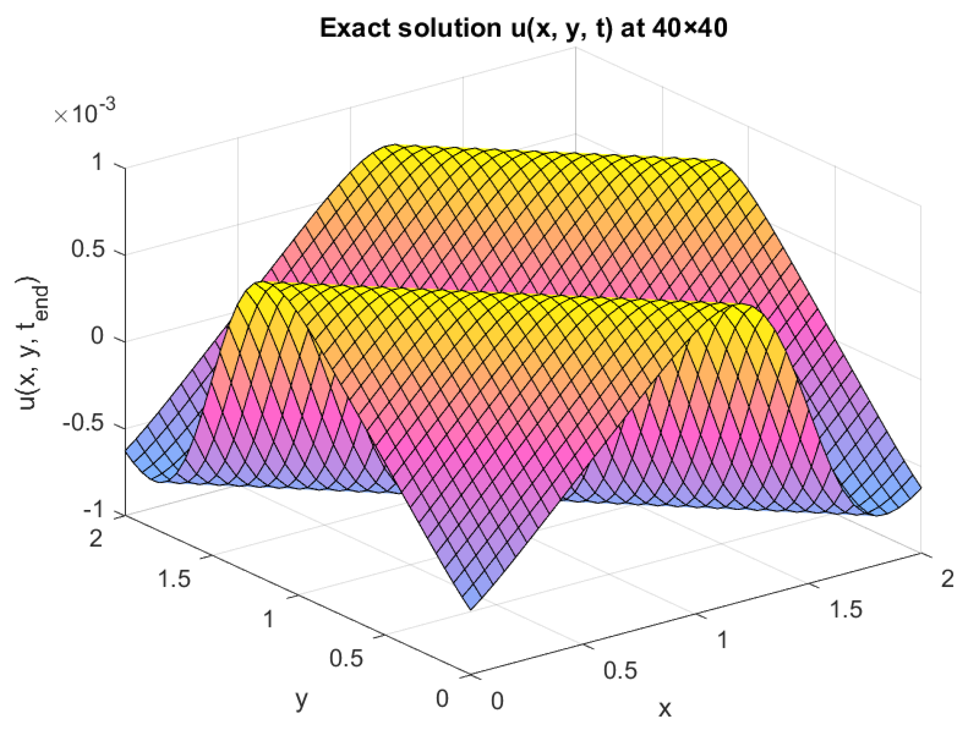
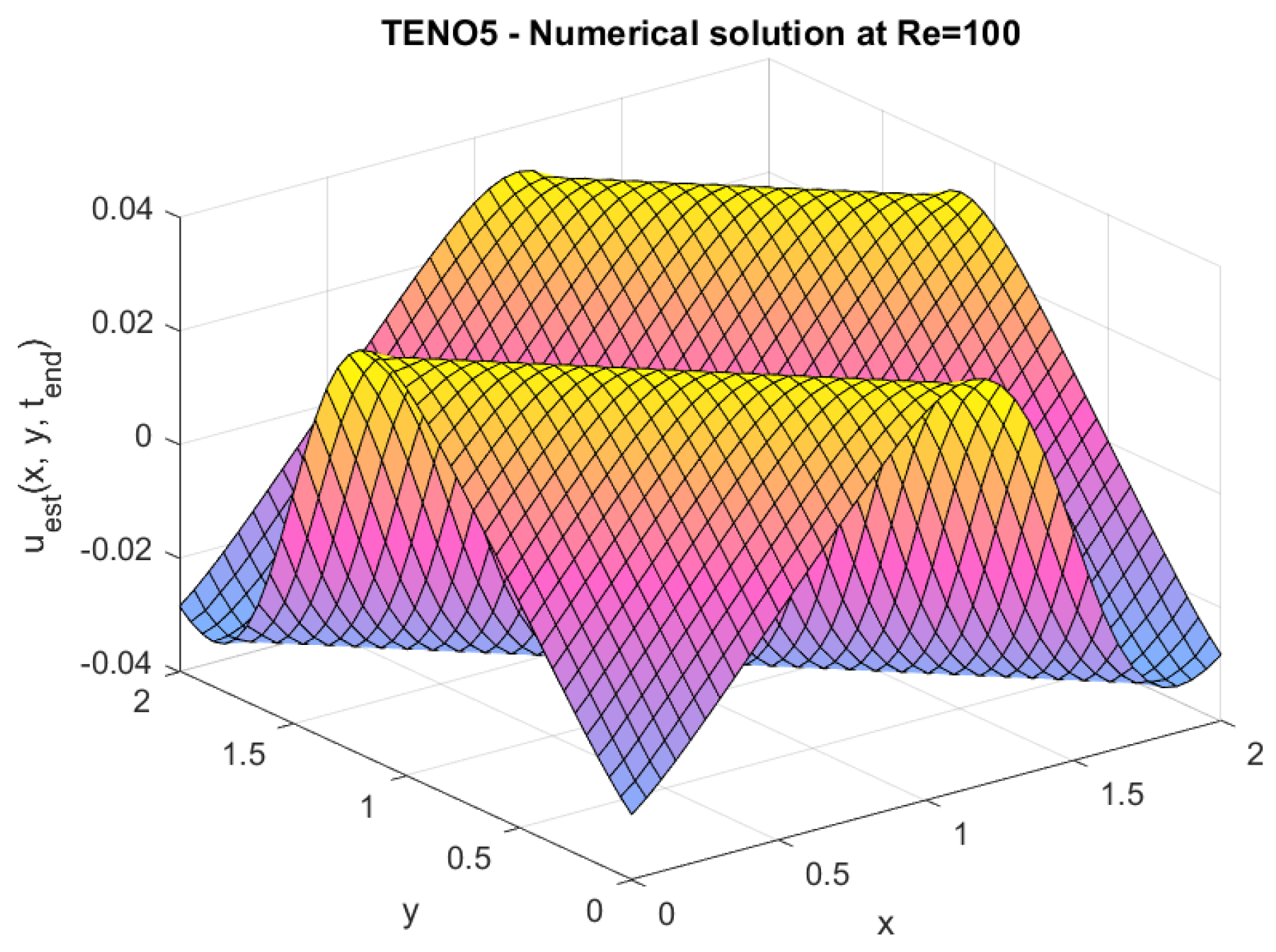
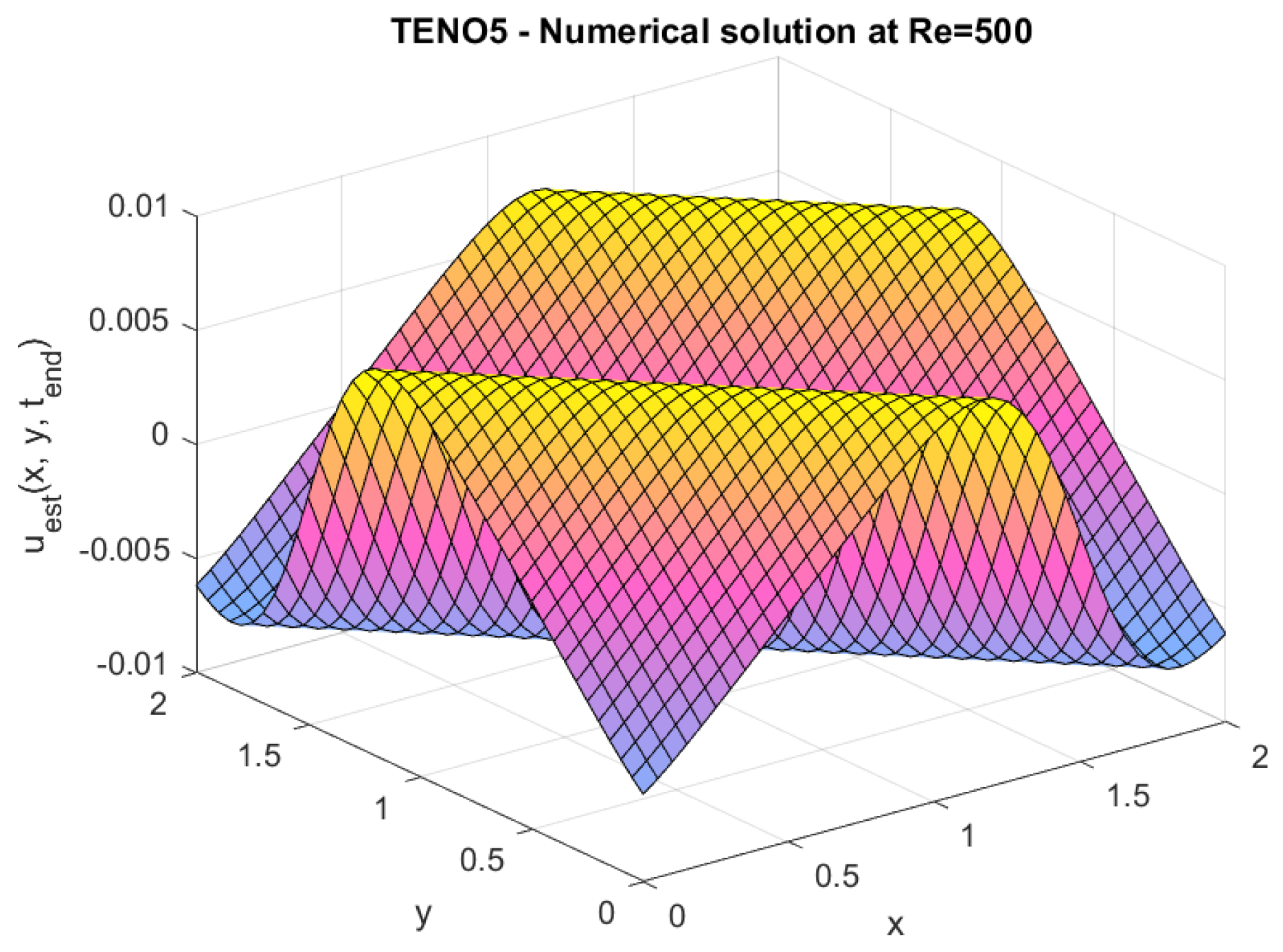
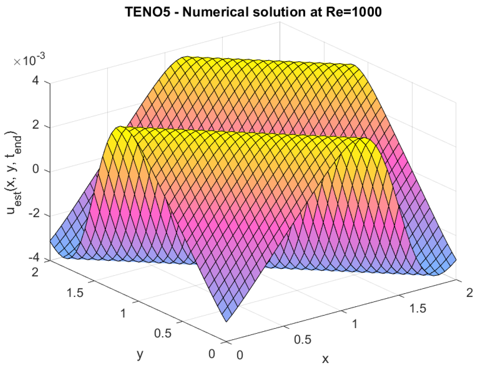
3.2. Burgers’ Equation with Diffusion

Consider the two-dimensional Burgers’ equation with diffusion

$$u_t+a\left[{\left({\displaystyle \frac{u^2}{2}}\right)}_x+{\left({\displaystyle \frac{u^2}{2}}\right)}_y\right]-D\left(u_{xx}+u_{yy}\right)=0.$$

(23)

on the domain ${[0,2]}^2$.

When $a=1$, the exact solution is given as

$$u(x,y,t)=-2D\pi {\displaystyle \frac{cos\left(\pi (x+y)\right)exp\left(-2D{\pi }^{2}t\right)}{2+sin\left(\pi (x+y)\right)exp\left(-2D{\pi }^{2}t\right)}}.$$

(24)

with $\mathrm{CFL}=0.5$, and at the final time, $t_{\mathrm{end}}=0.5$.

In this context, the diffusion coefficient, denoted as D, is given by the equation $D={\displaystyle \frac{1}{Re}}$, where $Re$ indicates the Reynolds number. In addition, different grid sizes are considered in this experiment, as represented in

Table 2. Error analysis of the TENO5 scheme in the FVM framework for a diffusion coefficient of D = 0.0002 with CFL = 0.5.

Nx × Ny	Error Type	TENO5
20 × 20	L1 error	4.1892 × 10−8
	L2 error	6.7318 × 10−8
	L∞ error	1.8217 × 10−7
40 × 40	L1 error	1.2546 × 10−8
	L2 error	2.0612 × 10−8
	L∞ error	5.8097 × 10−8
80 × 80	L1 error	5.8603 × 10−9
	L2 error	9.967 × 10−9
	L∞ error	5.9789 × 10−8
160 × 160	L1 error	7.9686 × 10−9
	L2 error	1.1022 × 10−8
	L∞ error	3.2989 × 10−8

. The plots in this paper are specifically for a 40 × 40 uniform grid (

Table 3. Error analysis for TENO5 in the FVM framework at various Reynolds numbers, performed on a 40 × 40 uniform grid with CFL = 0.5.

Error Type	Re = 50	Re = 100	Re = 500	Re = 1000
L1 error	0.0028585	0.00034326	2.7898 × 10−6	4.006 × 10−7
L2 error	0.0051578	0.00046317	4.1123 × 10−6	6.1714 × 10−7
L∞ error	0.019154	0.00094257	1.2755 × 10−5	2.2067 × 10−6

).

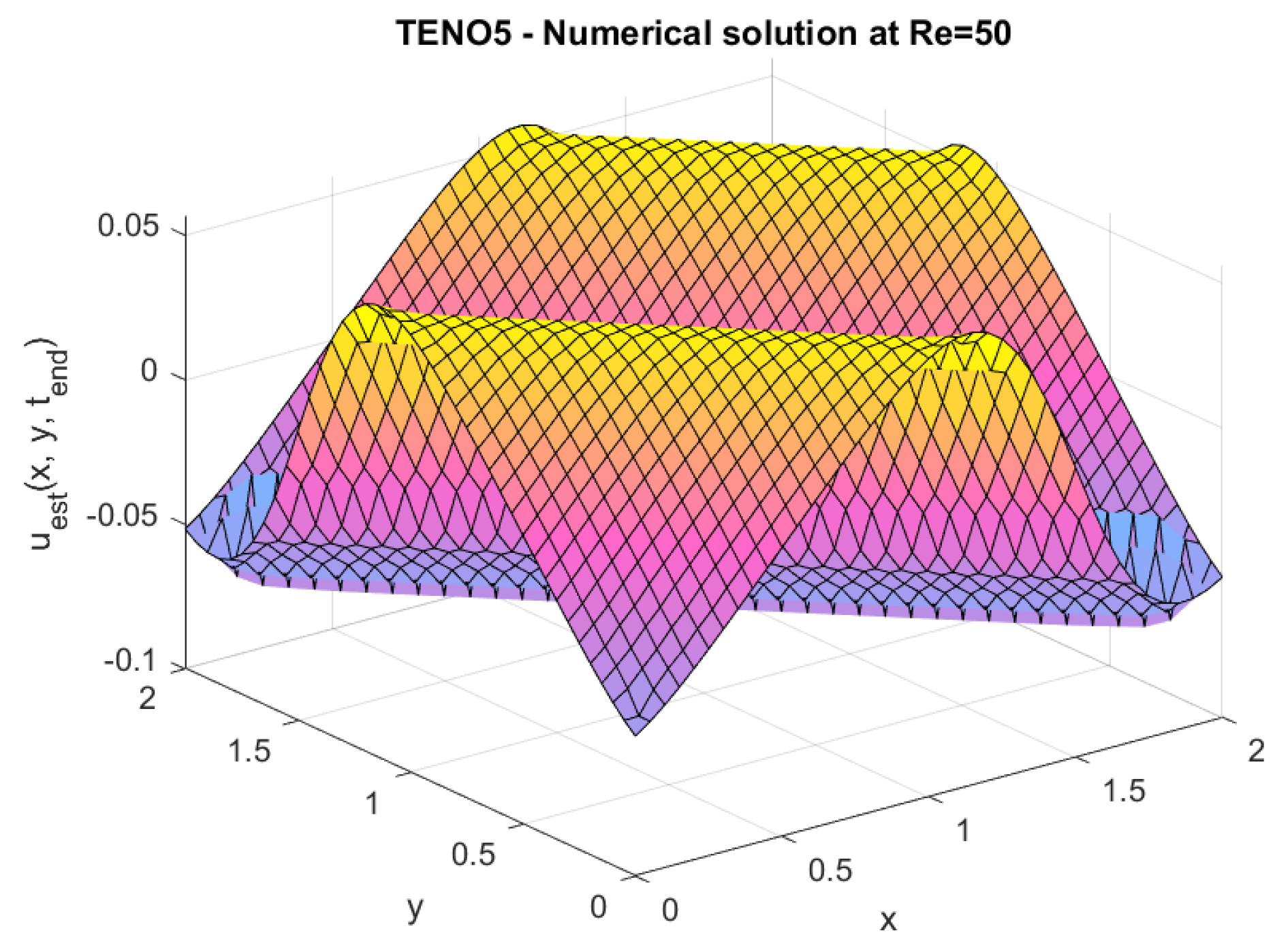
This work also incorporates an additional study that investigates the performance of the TENO5 scheme at different Reynolds numbers ($\mathrm{Re}$) to examine its suitability within the FVM framework.

The Reynolds number ($\mathrm{Re}$) is an important dimensionless number in fluid dynamics that determines the relative importance of the inertial to viscous force in the system.

At low $\mathrm{Re}$, viscous effects outweigh inertial effects, and the flow is smooth, while at high $\mathrm{Re}$, inertial forces are larger, and the flow becomes turbulent or has sharp gradients.

Numerical simulations, which were aimed at investigating the performance of TENO5 in handling a flow regime and simulating both the sharp and smooth features at different $\mathrm{Re}$, were made to study its potential. The purpose of these tests was to determine the general operation of the scheme in a wide range of flows and to check the stability and accuracy of the solution in a smooth and complex flow.

The numerical results of these experiments are given below.

4. Discussion

The numerical experiments presented in Section 3 illustrate the efficacy of the TENO5 scheme in addressing both linear and nonlinear issues within a finite volume context. The examination focuses on the advection of multiple waveforms and the two-dimensional Burgers’ equation incorporating diffusion. The subsequent subsections discuss the accuracy, convergence behavior, and performance of the numerical method.

4.1. Effect of Final Time Integration, CFL Number, Reynolds Number, and Grid Resolution

In the present study, we use a final simulation time of $t_{\mathrm{end}}=0.5$ and a CFL number of 0.5, and we consider Reynolds numbers of Re = 50, 100, 500, 1000, and 5000. So, $D={\displaystyle \frac{1}{\mathrm{Re}}}$, e.g., D = 0.0002 at Re = 5000. In addition to their direct effect, these attributes need to be accounted for in coordination with spatial resolution. Before moving on, we highlight its relationship to the number of grid points and grid optimization.

• Final simulation time (t_end): A larger $\mathrm{\Delta }t$ means that it takes more steps to reach its location (as $\mathrm{\Delta }t$ is controlled by CFL), and it also amplifies the effect of spatial discretization errors. For coarser meshes, error propagation and numerical diffusion are more dominant over the long run; so when t_end is increased, one should ensure that the mesh (increasing $N_x$) is refined such that the target accuracy is maintained.
  The error analysis of the TENO5 scheme for the two experiments at different t_end is shown in

  Table 4. Error analysis for the one-dimensional linear advection of multiple waves using TENO5 in the FVM framework at different $t_{\mathrm{end}}$, performed on a a uniform grid consisting of 200 points, with CFL = 0.5.

  Error Type	${\mathit{t}}_{\mathbf{end}}=0.5$	${\mathit{t}}_{\mathbf{end}}=1.0$	${\mathit{t}}_{\mathbf{end}}=1.5$	${\mathit{t}}_{\mathbf{end}}=2.0$	${\mathit{t}}_{\mathbf{end}}=2.5$
  L1 error	0.027077	0.10487	0.18209	0.28088	0.32118
  L2 error	0.070048	0.26756	0.3707	0.45204	0.49381
  L∞ error	0.327	1.0053	1.0111	1.0122	1.0129

  and

  Table 5. Error analysis for two-dimensional Burgers’ equation using TENO5 in the FVM framework at different t_end, performed on a 40 × 40 uniform grid with CFL = 0.5 and Re = 5000.

  Error Type	tend = 0.5	tend = 1.0	tend = 1.5	tend = 2.0	tend = 2.5
  L1 error	1.2546 × 10−8	2.5416 × 10−8	4.0946 × 10−8	5.9112 × 10−8	8.012 × 10−8
  L2 error	2.0612 × 10−8	4.1019 × 10−8	6.4118 × 10−8	9.0932 × 10−8	1.2343 × 10−7
  L∞ error	5.8097 × 10−8	1.2983 × 10−7	2.1927 × 10−7	3.2275 × 10−7	4.4134 × 10−7

  . The results indicate that the $L_1$, $L_2$, and $L_{\infty }$ errors significantly increase as the t_end rises. Therefore, there is an accumulation of errors.
  Hence, the determination of t_end is influenced by the selected experiment and other factors, such as parameters and diffusion.
• Courant–Friedrichs–Lewy number (CFL): To simplify the method, the CFL condition in one dimension can be stated as follows: $\mathrm{\Delta }t={\displaystyle \frac{\mathrm{CFL}\mathrm{\Delta }x}{c}}$. For a specific CFL = 0.5, the decrease in the cell size Δx (increasing the number of cells $N_x$) splits Δt in half, which means that terms proceed through twice as many time steps, and consequently, the temporal and the spatial truncations are reduced. Conversely, when using extremely fine meshes, one can wisely raise the CFL to a maximum of 0.5 to lower overall expenses, though this comes at the cost of stability.
  The error analysis of the TENO5 scheme for the linear advection of multiple waves, with various CFL, is presented in

  Table 6. Error analysis for the one-dimensional linear advection of multiple waves using TENO5 in the FVM framework with different CFL, performed on a a uniform grid consisting of 200 points, at t_end = 0.5.

  Error Type	CFL = 0.5	CFL = 1.0	CFL = 1.5	CFL = 2.0	CFL = 2.5
  L1 error	0.027077	0.027251	0.027077	0.035564	0.04933
  L2 error	0.070048	0.072087	0.071968	0.08464	0.10223
  L∞ error	0.327	0.34092	0.34508	0.40645	0.4416

  . The results indicate that the L₁, L₂, and L_∞ errors significantly increase as the CFL rises, and the determination of the CFL is also influenced by the selected experiment and other factors such as parameters.
  In the linear advection of multiple waves, errors and plot profiles are sharply and strongly influenced by the CFL number as the scheme must accurately follow wave propagation over many periods. A better temporal resolution and minimum phase error can be achieved for a lower CFL number.
  Moreover, for the two-dimensional Burgers’ equation with diffusion, diffusion has a smoothing effect since it removes small-scale oscillations and the dependence on the time step’s size. Because the solution is smooth and decaying, temporal errors are much smaller than spatial errors.
  In addition, with a short final time (e.g., t_end = 0.5), the time error dictated by the CFL is negligible.
• Reynolds number (Re) and diffusion coefficient (D): The diffusion coefficient spans, in fact, from $D={\displaystyle \frac{1}{\mathrm{Re}}}$. With the Re value increasing, the physical diffusion becomes smaller, and as a result, the gradients of density become sharper such that a finer spatial resolution is needed. For a higher Re, a refined mesh is still needed to capture these steep features and fully exploit the low-dissipation nature of the TENO5 scheme for D = 0.0002 at 5000 (as well as higher Re).
• Grid optimization strategy:
  To keep an acceptable balance between accuracy and efficiency, the choices of (t_end, CFL, Re, and N_x) should be implemented concurrently.
  In practice, it is common to use CFL to ensure stability. A grid convergence test is conducted by increasing N_x, based on which the error norms tend to stabilize. For a larger Re or longer t_end, additional finer meshes are necessary to resolve sharper gradients. This formulation guarantees accurate results and enables TENO5 to demonstrate its formal fifth-order convergence.

4.2. Linear Advection of Multiple Waves

The linear advection scenario involves a variety of waveforms, such as a Gaussian pulse, a square wave, a sharp triangle wave, and a half ellipse, that propogate without distortion according to governing Equation (18). Figure 1, Figure 2, Figure 3 and Figure 4 depict the numerical solution achieved with the TENO5 scheme in comparison to the exact solution at t_end = 0.5. The numerical findings show a strong correlation with the exact solution, especially in accurately capturing smooth areas of the waves. Nonetheless, minor numerical dissipation and dispersion effects are noted around discontinuities and sharp gradients, which is typical for high-order schemes dealing with discontinuous issues.

The error analysis illustrated in Table 1 verifies that the numerical error diminishes as the grid becomes finer. The L₁ and L₂ errors consistently decrease with enhanced resolutions, indicating that the scheme attains high-order accuracy in smooth regions. However, the L_∞ error does not decrease as smoothly as the other norms, implying that the maximum error remains localized around discontinuities where numerical oscillations might arise. These results suggest that TENO5 achieves commendable accuracy while effectively managing spurious oscillations.

4.3. Two-Dimensional Burgers’ Equation with Diffusion

Regarding the two-dimensional Burgers’ equation with diffusion, the findings expose the scheme’s capacity to accurately capture the complexities of nonlinear advection–diffusion behavior. Figure 5 and Figure 6 contrast the exact solution and the numerical solution for a diffusion coefficient of D = 0.0002 and Reynolds number of Re = 5000. The TENO5 scheme successfully reflects the solution structure with minimal numerical artifacts, even when using a relatively coarse 40 × 40 grid.

The error analysis in Table 2 shows that enhancements in the grid’s resolution lead to a significant drop in numerical errors. The L₁, L₂, and L_∞ errors decrease with grid refinement, corroborating the convergence of the scheme. Furthermore, the results presented in Figure 7, Figure 8, Figure 9 and Figure 10 reveal how varying Reynolds numbers affect the numerical solution. As the Reynolds number escalates, sharper gradients and more defined features appear in the solution. The TENO5 scheme adeptly resolves these characteristics, affirming its robustness in managing advection-dominated flows.

The error analysis across different Reynolds numbers, as outlined in Table 3, reinforces these findings. The scheme retains its accuracy across various flow regimes, with slight differences in numerical errors resulting from increased sharpness in the solution at higher Reynolds numbers. This indicates that the scheme effectively balances numerical dissipation while resolving steep gradients.

5. Conclusions

This research evaluates the TENO5 scheme within a finite volume context for problems dominated by advection. Numerical tests on both linear and nonlinear cases reveal its precision, reliability, and convergence. The TENO5 scheme successfully captures smooth wave patterns in linear advection scenarios while maintaining low dissipation and dispersion errors, even though there are slight oscillations near discontinuities. In the case of the two-dimensional Burgers’ equation with diffusion, it effectively addresses nonlinear dynamics at elevated Reynolds numbers and exhibits consistent convergence with grid refinement.

In summary, the TENO5 scheme demonstrates itself to be a very efficient method for problems driven by advection, striking a balance between numerical dissipation and resolution. Future research could broaden this study to encompass more intricate test cases, such as turbulent flows and multi-dimensional nonlinear systems. Moreover, examining higher-order extensions of the TENO framework could further improve accuracy, especially for issues involving fine-scale structures and turbulence. The extension to three-dimensional settings may provide some valuable insight into the performance and robustness properties of the scheme under increased complexity. However, there are difficulties in increased computational cost and the construction of the stencil in three dimensions.

References

1. Moukalled, F.; Mangani, L.; Darwish, M.; Moukalled, F.; Mangani, L.; Darwish, M. The Finite Volume Method; Springer: Berlin/Heidelberg, Germany, 2016. [Google Scholar]
2. Petrova, R. Finite Volume Method: Powerful Means of Engineering Design; BoD—Books on Demand: Norderstedt, Germany, 2012. [Google Scholar]
3. Liang, S. Numerical Simulation of the Navier-Stokes Equations Using Finite Volume Method. Master’s Thesis, Universitat Politècnica de Catalunya, Barcelona, Spain, 2017. [Google Scholar]
4. van Gestel, R.A.M. The Finite Volume Method for Systems of Conservation Laws. Master’s Thesis, Eindhoven University of Technology, Eindhoven, The Netherlands, 2019. [Google Scholar]
5. Savović, S.; Ivanović, M.; Drljača, B.; Simović, A. Numerical Solution of the Sine—Gordon Equation by Novel Physics-Informed Neural Networks and Two Different Finite Difference Methods. Axioms 2024, 13, 872. [Google Scholar] [CrossRef]
6. Savović, S.; Ivanović, M.; Min, R. A Comparative Study of the Explicit Finite Difference Method and Physics-Informed Neural Networks for Solving the Burgers’ Equation. Axioms 2023, 12, 982. [Google Scholar] [CrossRef]
7. Hadzic, H. Development and Application of Finite Volume Method for the Computation of Flows Around Moving Bodies on Unstructured, Overlapping Grids. Ph.D. Thesis, Hamburg University of Technology, Hamburg, Germany, 2006. [Google Scholar]
8. Zhang, Q.; Johansen, H.; Colella, P. A fourth-order accurate finite-volume method with structured adaptive mesh refinement for solving the advection-diffusion equation. SIAM J. Sci. Comput. 2012, 34, B179–B201. [Google Scholar] [CrossRef]
9. Jasak, H.; Tukovic, Z. Automatic mesh motion for the unstructured finite volume method. Trans. FAMENA 2006, 30, 1–20. [Google Scholar]
10. Fu, L. A low-dissipation finite-volume method based on a new TENO shock-capturing scheme. Comput. Phys. Commun. 2019, 235, 25–39. [Google Scholar] [CrossRef]
11. Huang, H.; Fu, L. A new troubled cell indicator and a new limiter based on TENO schemes for RKDG methods. Comput. Methods Appl. Mech. Eng. 2024, 421, 116795. [Google Scholar] [CrossRef]
12. Ji, Z.; Liang, T.; Fu, L. A class of new high-order finite-volume TENO schemes for hyperbolic conservation laws with unstructured meshes. J. Sci. Comput. 2022, 92, 61. [Google Scholar] [CrossRef]
13. Chandrashekar, P. Numerical Methods for Hyperbolic System of Conservation Laws; Tata Institute of Fundamental Research: Bangalore, India, 2019. [Google Scholar]
14. Tann, S.; Deng, X.; Shimizu, Y.; Loubère, R.; Xiao, F. Solution property preserving reconstruction for finite volume scheme: A bvd+ mood framework. Int. J. Numer. Methods Fluids 2019. [Google Scholar]
Figure 1. One-dimensional linear advection of multiple waves, comparing the exact solution and the numerical solution using the TENO5 scheme at simulation time t end = 0.5 . Spatial discretization is on N x = 25 uniform grid points with CFL = 0.5 .
Axioms 14 00359 g001
Figure 2. One-dimensional linear advection of multiple waves, comparing the exact solution and the numerical solution using the TENO5 scheme at simulation time t end = 0.5 . Spatial discretization is on N x = 50 uniform grid points with CFL = 0.5 .
Axioms 14 00359 g002
Figure 3. One-dimensional linear advection of multiple waves, comparing the exact solution and the numerical solution using the TENO5 scheme at simulation time t end = 0.5 . Spatial discretization is on N x = 100 uniform grid points with CFL = 0.5 .
Axioms 14 00359 g003
Figure 4. One-dimensional linear advection of multiple waves, comparing the exact solution and the numerical solution using the TENO5 scheme at simulation time t end = 0.5 . Spatial discretization is on N x = 200 uniform grid points with CFL = 0.5 .
Axioms 14 00359 g004
Figure 5. Exact solution of the two-dimensional Burgers’ equation with diffusion. The value of the diffusion coefficient is D = 0.0002 and associated with Re = 5000 , with a CFL = 0.5 . The domain is discretized using a 40 × 40 uniform grid.
Axioms 14 00359 g005
Figure 6. Numerical solution of the two-dimensional Burgers’ equation with diffusion. The value of the diffusion coefficient is D = 0.0002 and is associated with Re = 5000 , with a CFL = 0.5 . The domain is discretized using a 40 × 40 uniform grid.
Axioms 14 00359 g006
Figure 7. Numerical solution of the two-dimensional Burgers’ equation with diffusion. The value of the diffusion coefficient is D = 0.02 and is associated with Re = 50 , with a CFL = 0.5 . The domain is discretized using a 40 × 40 uniform grid.
Axioms 14 00359 g007
Figure 8. Numerical solution of the two-dimensional Burgers’ equation with diffusion. The value of the diffusion coefficient is D = 0.01 and is associated with Re = 100 , with a CFL = 0.5 . The domain is discretized using a 40 × 40 uniform grid.
Axioms 14 00359 g008
Figure 9. Numerical solution of the two-dimensional Burgers’ equation with diffusion. The value of the diffusion coefficient is D = 0.002 and is associated with Re = 500 , with a CFL = 0.5 . The domain is discretized using a 40 × 40 uniform grid.
Axioms 14 00359 g009
Figure 10. Numerical solution of the two-dimensional Burgers’ equation with diffusion. The value of the diffusion coefficient is D = 0.001 and is associated with Re = 1000 , with a CFL = 0.5 . The domain is discretized using a 40 × 40 uniform grid.
Axioms 14 00359 g010