
Numerical Simulations for Parabolic Stochastic Equations Using a Structure-Preserving Local Discontinuous Galerkin Method


Abstract
1. Introduction
- (1)
- For , the increment is normally distributed with mean zero and variance .
- (2)
- is a continuous square-integrable martingale and its quadratic variation for all .
- (3)
- Let , the family of -valued -adapted processes such that and mathematical expectation , then is -measurable and .
2. Preliminaries
3. The Construction of the LDG Method
4. Stability and Conservation Property
5. Error Estimation Analysis
- The estimate of .
- The estimate of .
- The estimate of .
- The estimate of .where max .
- The estimate of .
- The estimate of .
6. Numerical Experiments
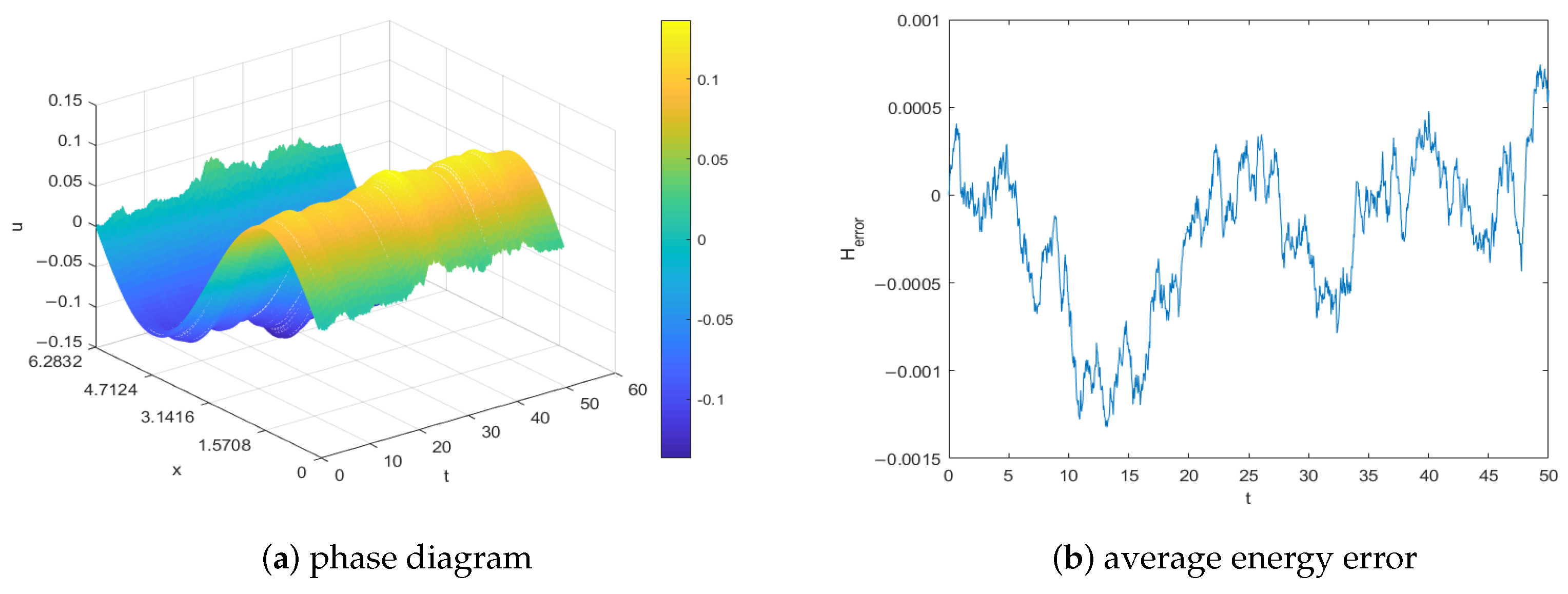
6.1. Example 1
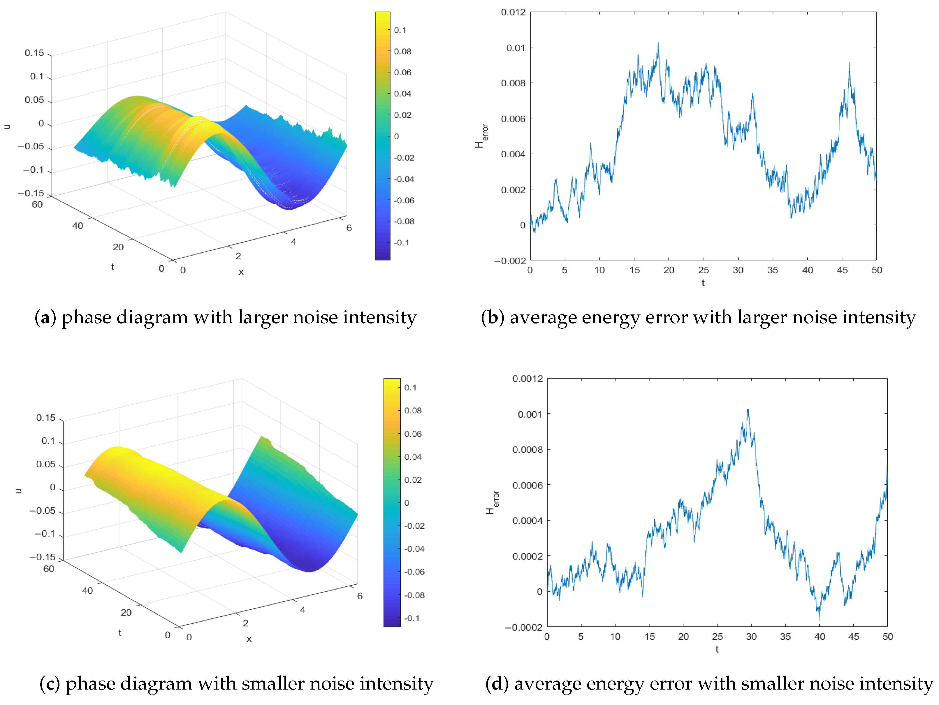
6.2. Example 2
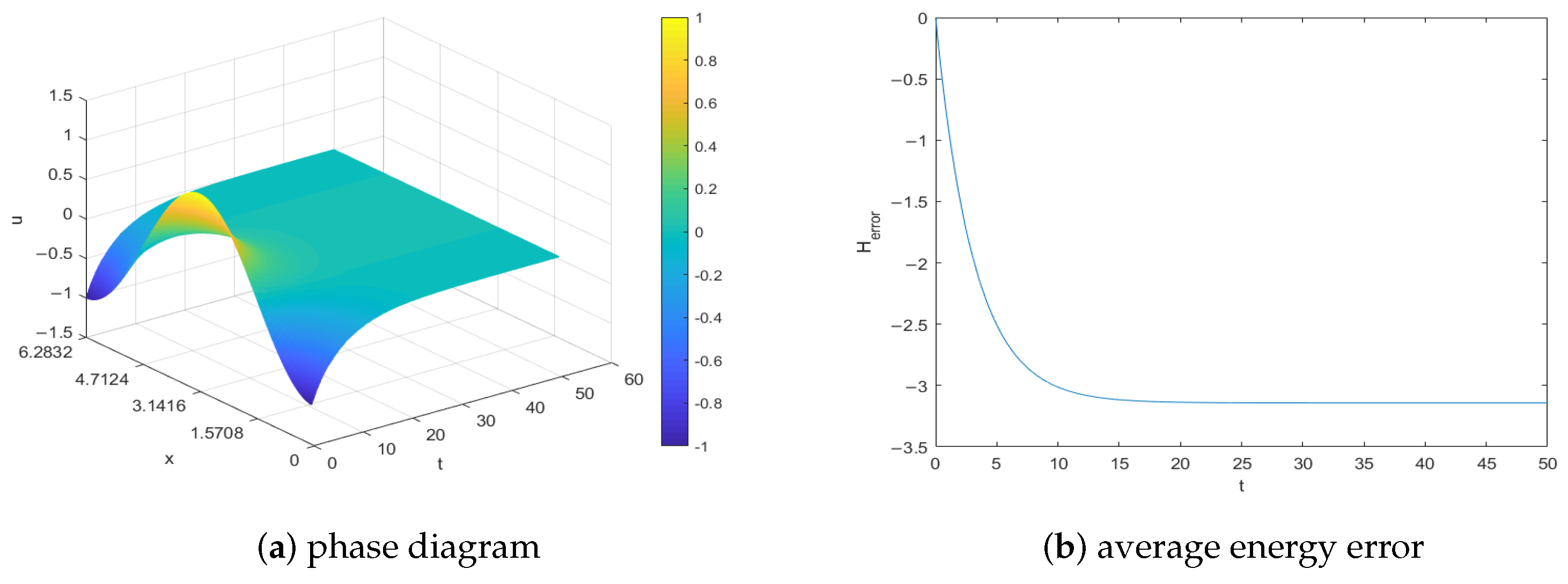
6.3. Example 3
7. Conclusions
Author Contributions
Funding
Data Availability Statement
Acknowledgments
Conflicts of Interest
References
- Liu, T. Porosity reconstruction based on Biot elastic model of porous media by homotopy perturbation method. Chaos Solitons Fractals 2022, 158, 112007. [Google Scholar] [CrossRef]
- Liu, T.; Li, T.; Ullah, M.Z. On five-point equidistant stencils based on Gaussian function with application in numerical multi-dimensional option pricing. Comput. Math. Appl. 2024, 176, 11. [Google Scholar] [CrossRef]
- Khattab, A.G.; Semary, M.S.; Hammad, D.A.; Fathy, A. Exploring stochastic heat equations: A numerical analysis with fast discrete Fourier transform techniques. Axioms 2024, 13, 886. [Google Scholar] [CrossRef]
- Fareed, A.F.; Semary, M.S. Stochastic improved Simpson for solving nonlinear fractional-order systems using product integration rules. Nonlinear Eng. 2025, 14, 20240070. [Google Scholar] [CrossRef]
- Fareed, A.F.; Semary, M.S.; Hassan, H.N. Two semi-analytical approaches to approximate the solution of stochastic ordinary differential equations with two enormous engineering applications. Alex. Eng. J. 2022, 61, 11935–11945. [Google Scholar] [CrossRef]
- Arif, M.S.; Abodayeh, K.; Nawaz, Y. A reliable computational scheme for stochastic reaction–diffusion nonlinear chemical model. Axioms 2023, 12, 460. [Google Scholar] [CrossRef]
- Arif, M.S.; Abodayeh, K.; Nawaz, Y. A computational scheme for stochastic non-Newtonian mixed convection nanofluid flow over oscillatory sheet. Energies 2023, 16, 2298. [Google Scholar] [CrossRef]
- Nawaz, Y.; Arif, M.S.; Nazeer, A.; Abbasi, J.N.; Abodayeh, K. A two-stage reliable computational scheme for stochastic unsteady mixed convection flow of Casson nanofluid. Int. J. Numer. Methods Fluids 2024, 96, 719–737. [Google Scholar] [CrossRef]
- Babaei, A.; Banihashemi, S.; Moghaddam, B.P.; Dabiri, A.; Galhano, A. Efficient solutions for stochastic fractional differential equations with a neutral delay using Jacobi poly-fractonomials. Mathematics 2024, 12, 3273. [Google Scholar] [CrossRef]
- Aryani, E.; Babaei, A.; Valinejad, A. A numerical technique for solving nonlinear fractional stochastic integro-differential equations with n-dimensional Wiener process. Comput. Methods Differ. Equ. 2022, 10, 61–76. [Google Scholar]
- Liu, T.; Ding, B.; Saray, B.N.; Juraev, D.A.; Elsayed, E.E. On the pseudospectral method for solving the fractional Klein–Gordon equation using Legendre cardinal functions. Fractal Fract. 2025, 9, 177. [Google Scholar] [CrossRef]
- Liu, T. Parameter estimation with the multigrid-homotopy method for a nonlinear diffusion equation. J. Comput. Appl. Math. 2022, 413, 114393. [Google Scholar] [CrossRef]
- Liu, Z.; Qiao, Z. Strong approximation of monotone stochastic partial differential equations driven by white noise. IMA J. Numer. Anal. 2020, 40, 1074–1093. [Google Scholar] [CrossRef]
- Mukam, J.D. Some Numerical Techniques for Approximating Semilinear Parabolic (Stochastic) Partial Differential Equations; Technische Universität Chemnitz: Chemnitz, Germany, 2021. [Google Scholar]
- Cui, J.; Hong, J. Strong and weak convergence rates of a spatial approximation for stochastic partial differential equation with one-sided Lipschitz coefficient. SIAM J. Numer. Anal. 2019, 57, 1815–1841. [Google Scholar] [CrossRef]
- Jin, B.; Yan, Y.; Zhou, Z. Numerical approximation of stochastic time-fractional diffusion. ESAIM Math. Model. Numer. Anal. 2019, 53, 1245–1268. [Google Scholar] [CrossRef]
- Peng, G.; Gao, Z.; Feng, X. A stabilized extremum-preserving scheme for nonlinear parabolic equation on polygonal meshes. Int. J. Numer. Methods Fluids 2019, 90, 340–356. [Google Scholar] [CrossRef]
- Yan, J.; Shu, C.W. Local discontinuous Galerkin methods for partial differential equations with higher order derivatives. J. Sci. Comput. 2002, 17, 27–47. [Google Scholar] [CrossRef]
- Chen, C.; Hong, J.; Ji, L. Mean-square convergence of a symplectic local discontinuous Galerkin method applied to stochastic linear Schrödinger equation. IMA J. Numer. Anal. 2017, 37, 1041–1065. [Google Scholar] [CrossRef]
- Li, Y. A high-order numerical method for BSPDEs with applications to mathematical finance. SIAM J. Financ. Math. 2022, 13, 147–178. [Google Scholar] [CrossRef]
- Li, Y. A high-order numerical scheme for stochastic optimal control problem. J. Comput. Appl. Math. 2023, 427, 115158. [Google Scholar] [CrossRef]
- Wang, H.; Tao, Q.; Shu, C.W.; Zhang, Q. Analysis of local discontinuous Galerkin methods with implicit-explicit time marching for linearized KdV equations. SIAM J. Numer. Anal. 2024, 62, 2222–2248. [Google Scholar] [CrossRef]
- Zhang, L.; Ji, L. Stochastic multi-symplectic Runge–Kutta methods for stochastic Hamiltonian PDEs. Appl. Numer. Math. 2019, 135, 396–406. [Google Scholar] [CrossRef]
- Zhou, Y.; Wang, Q.; Zhang, Z. Physical properties preserving numerical simulation of stochastic fractional nonlinear wave equation. Commun. Nonlinear Sci. Numer. Simul. 2021, 99, 105832. [Google Scholar] [CrossRef]
- Hou, B. Meshless structure-preserving GRBF collocation methods for stochastic Maxwell equations with multiplicative noise. Appl. Numer. Math. 2023, 192, 337–355. [Google Scholar] [CrossRef]
- Bai, G.; Hu, J.; Li, B. High-Order mass-and energy-conserving methods for the nonlinear Schrödinger equation. SIAM J. Sci. Comput. 2024, 46, A1026–A1046. [Google Scholar] [CrossRef]
- Mao, X. Stochastic Differential Equations and Their Applications; Harwood: Chichester, UK, 1997. [Google Scholar] [CrossRef]
- Kuo, H.H. Introduction to Stochastic Integration; Springer: New York, NY, USA, 2006. [Google Scholar] [CrossRef]
- He, S.W.; Wang, J.G.; Yan, J.A. Semimartingale Theory and Stochastic Calculus; Routledge: London, UK, 1992; p. 400. [Google Scholar]


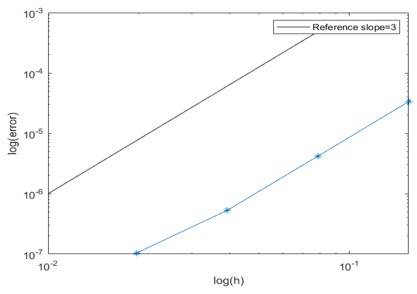
| h | Error | Order |
|---|---|---|
| – | ||
| 3.00 | ||
| 2.98 | ||
| 2.35 |
Disclaimer/Publisher’s Note: The statements, opinions and data contained in all publications are solely those of the individual author(s) and contributor(s) and not of MDPI and/or the editor(s). MDPI and/or the editor(s) disclaim responsibility for any injury to people or property resulting from any ideas, methods, instructions or products referred to in the content. |
© 2025 by the authors. Licensee MDPI, Basel, Switzerland. This article is an open access article distributed under the terms and conditions of the Creative Commons Attribution (CC BY) license (https://creativecommons.org/licenses/by/4.0/).
Share and Cite
Han, M.; Wang, Z.; Ding, X. Numerical Simulations for Parabolic Stochastic Equations Using a Structure-Preserving Local Discontinuous Galerkin Method. Axioms 2025, 14, 357. https://doi.org/10.3390/axioms14050357
Han M, Wang Z, Ding X. Numerical Simulations for Parabolic Stochastic Equations Using a Structure-Preserving Local Discontinuous Galerkin Method. Axioms. 2025; 14(5):357. https://doi.org/10.3390/axioms14050357
Chicago/Turabian StyleHan, Mengqin, Zhenyu Wang, and Xiaohua Ding. 2025. "Numerical Simulations for Parabolic Stochastic Equations Using a Structure-Preserving Local Discontinuous Galerkin Method" Axioms 14, no. 5: 357. https://doi.org/10.3390/axioms14050357
APA StyleHan, M., Wang, Z., & Ding, X. (2025). Numerical Simulations for Parabolic Stochastic Equations Using a Structure-Preserving Local Discontinuous Galerkin Method. Axioms, 14(5), 357. https://doi.org/10.3390/axioms14050357