Abstract
Two nonlinear Duffing equations are numerically treated in this article. The nonlinear fractional-order Duffing equations and the second-order nonlinear Duffing equations are handled. Based on the collocation technique, we provide two numerical algorithms. To achieve this goal, a new family of basis functions is built by combining the sets of Fibonacci and Lucas polynomials. Several new formulae for these polynomials are developed. The operational matrices of integer and fractional derivatives of these polynomials, as well as some new theoretical results of these polynomials, are presented and used in conjunction with the collocation method to convert nonlinear Duffing equations into algebraic systems of equations by forcing the equation to hold at certain collocation points. To numerically handle the resultant nonlinear systems, one can use symbolic algebra solvers or Newton’s approach. Some particular inequalities are proved to investigate the convergence analysis. Some numerical examples show that our suggested strategy is effective and accurate. The numerical results demonstrate that the suggested collocation approach yields accurate solutions by utilizing Fibonacci–Lucas polynomials as basis functions.
Keywords:
Fibonacci–Lucas polynomials; spectral methods; nonlinear Duffing equation; convergence analysis MSC:
65M70; 11B39
1. Introduction
For a wide variety of applications, special functions are essential. One can consult [1,2,3] for specific findings and uses of special functions. The Fibonacci and Lucas polynomials are important special functions [4]. A number of authors were keen on presenting and exploring various extensions and variations of these polynomials.
Research on generalized Lucas polynomials and their connections to Fibonacci and Lucas polynomials was covered in [5], whereas [6] focused on Gauss–Fibonacci and Gauss–Lucas polynomials and their uses. Additional contributions on these polynomials and their uses may be found in [7,8,9,10].
Finding different formulae for special functions is something that a number of mathematicians are interested in. The development of numerical approaches to solve different types of differential equations (DEs) can greatly benefit from these equations. Many approaches for solving different DEs using spectral methods require expressing the derivatives of special polynomials as combinations of their original ones. This approach has been used in previous works (see [11,12]). Furthermore, for any orthogonal or nonorthogonal polynomials, it is an important goal to construct the operational matrices for the derivatives of these polynomials. These operational matrices aid in transforming the DEs using an appropriate spectral approach into an algebraic system of equations that can be solved using appropriate linear algebra procedures; see [13,14,15,16,17].
Nonlinear DEs are indispensable in many scientific fields, including physics, biology, chemistry, economics, and engineering. These equations describe systems that are too complex to be described by linear equations. The study of nonlinear differential equations (DEs)—which are utilized to depict phenomena such as chaos, turbulence, and nonlinear waves—provides valuable insights that find widespread application in fields ranging from climate modeling and fluid dynamics to telecommunications (e.g., [18,19]).
Fractional differential equations (FDEs) are fundamental in a number of areas of the applied sciences. Standard DEs are unable to catch some events which they explain. This is due to their exceptional ability to mimic genetic and memory functions. For instance, as mentioned in [20], they mimic a variety of physiological and biological processes, such as neuronal activity and tumor formation. Since these equations cannot be solved analytically, numerical analysis typically comes into play while solving them. For instance, as demonstrated in [21], a collocation approach might be useful when dealing with several equations. Some of these approaches are referenced in [22,23,24].
Among the important nonlinear DEs are the different Duffing equations introduced by the engineer Georg Duffing in 1918. They arise in physics and engineering to model a variety of physical phenomena. Examples of these uses include the description of a system’s chaotic behavior [25] and the control of a chaotic system’s mobility around less complicated attractors by the injection of modest dampening signals [26]. Many authors were interested in handling the different Duffing equations. For example, the authors of [27] found analytical solutions for some Duffing equations. The author in [28] applied the Pell–Lucas approach to treating the Duffing equation. A machine learning was used in [29]. A certain Runge–Kutta approach was utilized in [30]. A general solution of the Duffing equation of third-order nonlinearity was proposed in [31]. In [32], the authors used an adapted block hybrid method to handle Duffing equations. To access many contributions about diverse forms of Duffing equations, one may refer to [33,34,35,36,37,38].
Spectral methods have become widely recognized as a significant class of numerical techniques for addressing various problems in different disciplines. These methods have many advantages comparable to various numerical methods (see [39]). The approximate solutions obtained by these methods are highly accurate and provide exponential convergence rates. In addition, unlike the finite element or finite difference method, they provide global solutions, not local ones. These methods are adaptable in treating different types of differentiable equations. We can choose the suitable method that we can use according to the type of differential equation and the type of underlying conditions. There are three main spectral methods. Every method has its advantages and uses. The Galerkin and Petrov–Galerkin methods can be applied successfully for linear problems and some specific nonlinear problems; see, for example, [40,41,42]. The Tau method has a wider range of applications than the Galerkin method due to its ability to handle more complex boundary conditions; for example, see [43,44,45]. The collocation method is advantageous, since it can handle any type of differential equation regulated with any type of underlying conditions, for example, [46,47,48,49,50].
In this paper, we are devoted to proposing two numerical algorithms to solve the second-order and fractional-order Duffing equations. The spectral collocation algorithm is applied for such a purpose. Moreover, a new set of basis functions that generalize the Fibonacci and Lucas basis are introduced and employed. To our knowledge, the basis functions introduced for our algorithm’s derivation are new. In what follows, we summarize the main points, including the novelty of our contribution in this paper:
- Introducing a new type of generalized Fibonacci and Lucas polynomials.
- Establishing some theoretical results concerning these polynomials that will be the backbone of our numerical results.
- Designing a numerical algorithm for treating the nonlinear second-order Duffing equation.
- Designing a numerical algorithm for treating the nonlinear fractional Duffing equation.
- Discussing the error analysis of the proposed method.
- Testing our algorithms numerically by presenting some numerical examples with some comparisons.
The advantages of our proposed technique can be summarized as follows:
- By choosing combined Fibonacci-Lucas polynomials as basis functions, a few retained modes produce highly accurate approximations.
- The approach requires fewer computations to achieve the desired precision.
- We can obtain several approximate solutions based on the presence of two free parameters, a and b.
- Our technique can treat both linear and non-linear equations.
Here is the outline of the paper: An overview of Fibonacci and Lucas polynomials is given in Section 2. In addition, a combined Fibonacci–Lucas class of polynomials is presented in this section. The nonlinear second-order Duffing problem is solved using a matrix collocation method in Section 3. In Section 4, the fractional-order Duffing equation is addressed using a collocation method. Section 5 discusses the expansion’s convergence and truncation error bound. Section 6 provides a few comparisons and examples. Some last thoughts are presented in Section 7.
2. Introducing a Unified Sequence of Fibonacci and Lucas Polynomials
This section discusses some essential features of Fibonacci and Lucas polynomials and introduces a unified sequence of Fibonacci and Lucas sequences.
2.1. Fibonacci and Lucas Polynomial Sequences
The Fibonacci and Lucas polynomial sequences can be generated using, respectively, the following two recursive formulas:
The generating function for is given by
while the generating function for is given by
For an approach for generating a function, one can refer to [51].
From (1) and (2), it is evident that both Fibonacci and Lucas polynomials satisfy the same recursive formula but with different initials; thus, it is clear that the following recurrence relation
generalizes the two sequences in (1) and (2), and we will denote , that is,
It is also clear that
We also have the following expressions
and their inverse expressions
where
Remark 1.
The key idea to develop the formulas concerned with the polynomials that satisfy (3) is the following theorem, in which we will show that may be expressed as a combination of two Fibonacci polynomials.
Theorem 1.
Consider any non-negative integer j. The polynomials can be represented as
Proof.
Consider the following polynomial:
It is clear that , and hence, it is sufficient to prove that satisfies the same recurrence relation of , for , that is, we are going to prove that
Using the recursive formula of the Fibonacci polynomials (1) in the form
along with the definition in (10), it can be shown that
This proves the theorem. □
The inverse connection formula of (9) is also interesting. The following theorem exhibits this result.
Theorem 2.
The Fibonacci polynomials are linked by Fibonacci–Lucas polynomials by the following two formulas:
Proof.
Theorem 3.
Consider a positive integer k. The power for representation of is
Proof.
Remark 3.
Lemma 1.
The inversion formula of is
where
2.2. Derivatives and Operational Matrices of the Fibonacci–Lucas Polynomials
In this part, we will develop the high-order derivatives of the Fibonacci–Lucas polynomials and, after that, establish their operational matrices of integer derivatives, which will be pivotal in designing our numerical algorithm.
Theorem 4.
Consider two positive integers q and j with . The qth derivative of takes the form
where
and
and is defined as in (16).
Proof.
Now, if we consider the vector defined as
then based on Formula (19), we can write the following general derivative expression:
where is the general operational matrix of derivatives of order whose elements can be written in the following form:
For our subsequent purposes, it is necessary to compute the two operational matrices of derivatives for the two cases corresponding to and . The following corollary presents these results.
Corollary 1.
For , Formula (22) gives, respectively, the following two derivative expressions:
where and are operational matrices of derivatives of order whose elements can be written in the following form:
As an example, for , and take the following forms:
Remark 4.
The operational matrices of integer derivatives in (22) will play an essential role in deriving the proposed algorithm.
Remark 5.
After establishing the fundamental background for the combined Fibonacci–Lucas polynomials, they may be utilized in solving other types of differential equations, both linear and nonlinear, using the matrix approach.
Remark 6.
Although the Fibonacci and Lucas polynomials were utilized in several publications to act as basis functions in spectral methods, it is worth mentioning that our Fibonacci–Lucas polynomial basis has the advantage of merging both the Fibonacci and Lucas polynomial bases to obtain several approximate solutions.
3. A Matrix Collocation Approach for the Nonlinear Second-Order Duffing Equation
In this section, we consider the following nonlinear second-order Duffing equation (NSDE) [28,52]:
which is subject to the conditions
The main idea to solve (25) and (26) is to employ the operational matrices of the derivatives of , together with applying the collocation method.
- Now, let us define the following space function:
4. A Matrix Collocation Approach for the Nonlinear Fractional-Order Duffing Equation
This section is confined to presenting a numerical algorithm for treating the nonlinear fractional Duffing equation. First, some fundamental properties regarding the fractional calculus are mentioned below.
Definition 1
([53,54,55,56]). The Gerasimov–Caputo fractional derivative of order μ is defined as
where .
The operator satisfies the following properties for all :
where , and the notation denotes the ceiling function.
Now, consider the following nonlinear fractional-order Duffing equation (NFDE) [28,52]:
which is directed to the constraints
where
4.1. The Operational Matrix of Fractional Derivatives for
Theorem 5.
Proof.
The proof of this theorem can be divided into two cases corresponding to the value of k and :
Finally, Cases 1 and 2 may be joined in matrix form as
where the elements of the matrix are given in the following form:
This ends the proof of this theorem. □
4.2. Collocation Algorithm for the NFDE
Using similar procedures as in the preceding section, we can obtain the following residual based on Theorem 5:
As a result, we may obtain the following system of equations by using the collocation method:
where
The above system can be solved to obtain with the aid of the well-known Newton’s iterative method.
5. Error Bound
In this section, we aim to demonstrate that when N approaches infinity, and converge to zero. For the unknown function , we derive various error bounds and derivatives of this function.
Theorem 6.
Assume that , , let be the proposed approximate solution belonging to , and define
Consequently, this estimate holds:
Proof.
Consider the following Taylor expansion of about the point :
Because is the best approximation solution of , we have, using the idea of best approximation,
and therefore, we have
□
Theorem 7.
Suppose that and meet the assumption of Theorem 6 and
The following estimation holds:
Proof.
At the point , we can use the Taylor expansion of in (42) to write
Imitating similar steps as in Theorem 6 in accordance with the best approximation’s concept, one has
and this leads to
□
Theorem 8.
Suppose that , , and meet the assumption of Theorem 6 and
Then, the following estimation holds:
Proof.
Assume that is the Taylor expansion of about the point ; then, the residual between and can be written as
Since is the best approximate solution of , then according to the definition of the best approximation, we obtain
We obtain the desired result by performing steps as in Theorem 6. □
Theorem 9.
Assume that the Gerasimov–Caputo operator and the conditions of Theorem 6 hold. Then,
Proof.
□
Theorem 10.
Proof.
Theorem 11.
6. Illustrative Examples
Evaluation of our suggested collocation methods is the focus of this section. We solve a few test problems and present a few comparisons to ensure that our suggested methods are applicable and accurate.
The absolute errors (AEs) in the given tables are
Example 1
([28,52]). Consider the following NFDE:
which is subject to the conditions
and is selected in a way that makes the exact solution become
Equation (1) is solved using our proposed algorithm for and :
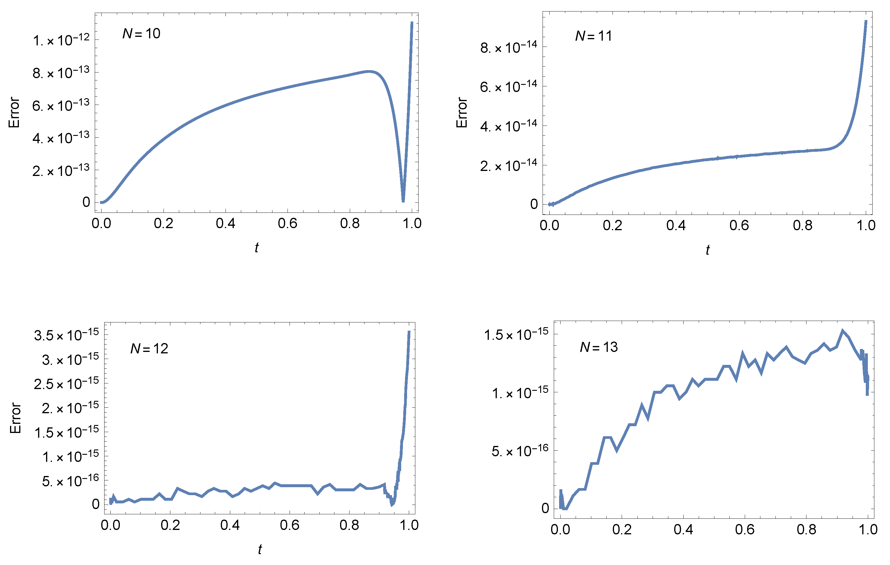
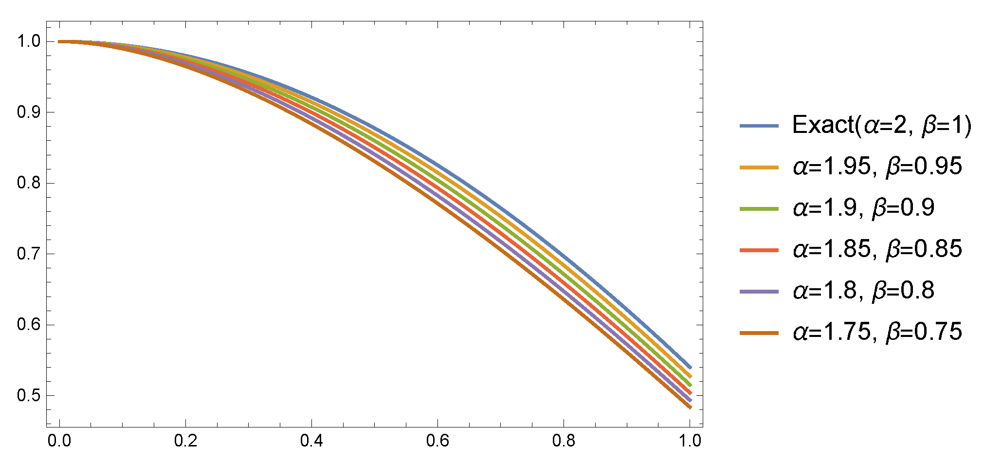
- Case 1: For and , Table 1 presents the AEs at different values of at when . Furthermore, Figure 1 shows the AEs at at different values of N when . Figure 2 shows that the approximate solutions have smaller variations for values of α and β near the values and when Table 2 presents the absolute errors (AEs) at different values of at when and .
 Table 1. AEs of Example 1 at .
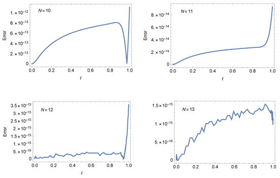 Figure 1. The AEs of Example 1 at .
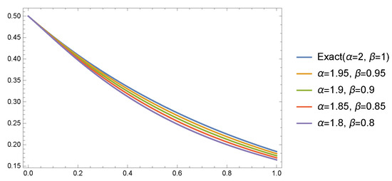 Figure 2. Different solutions of Example 1 at and different values of .
Table 2. AEs of Example 1 at .
Figure 2. Different solutions of Example 1 at and different values of .
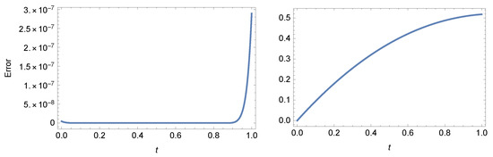
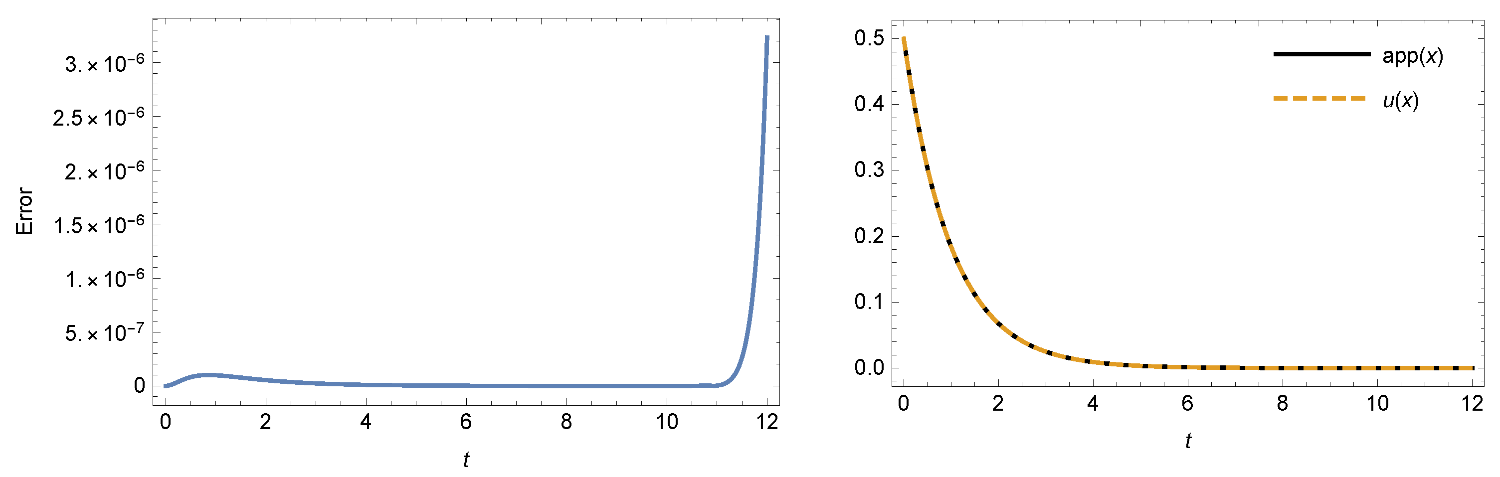
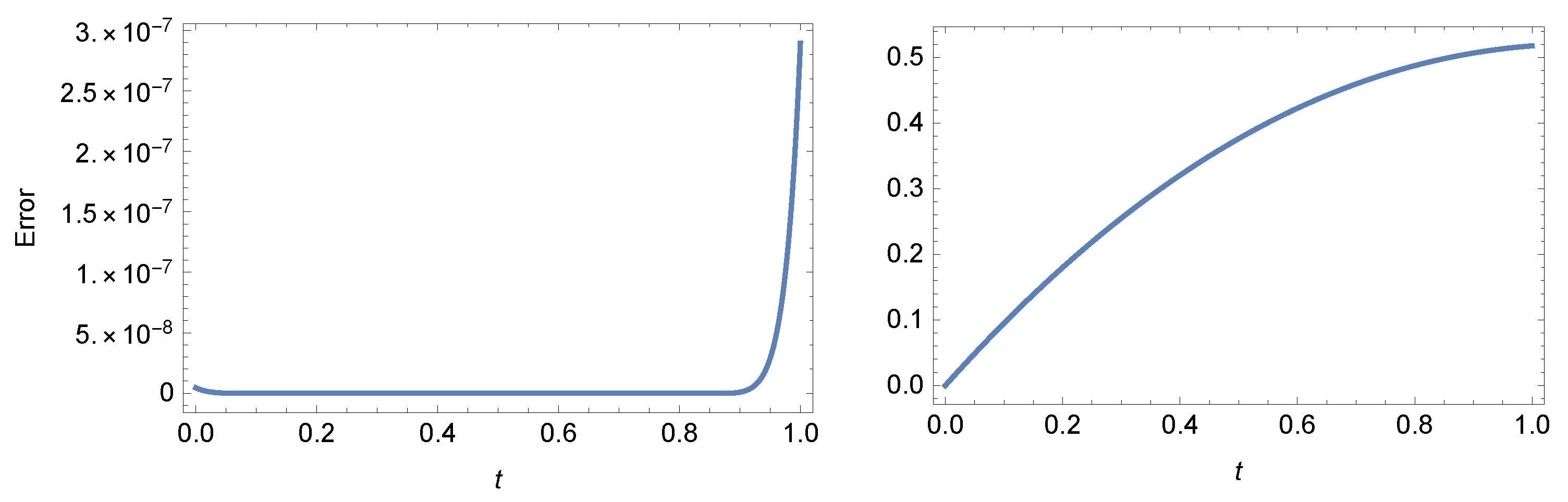
Table 2. AEs of Example 1 at . - Case 2: For , and , Table 3 presents a comparison between our method at and method in [52]. Figure 3 shows the AE (left) and exact, approximate solutions (right) of the example at and which demonstrates that the results of our method are extremely close to the exact solution.
Table 3. Comparison of AEs of Example 1 at .
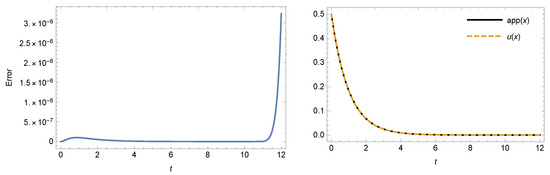 Figure 3. The AEs (left) and exact, approximate solutions (right) of Example 1 at and
Example 2
([52]). Consider the following NFDE:
which is subject to the conditions
and is selected in a way that makes the exact solution become at , where .
Equation (2) is solved using our algorithm for and :
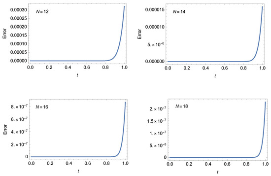
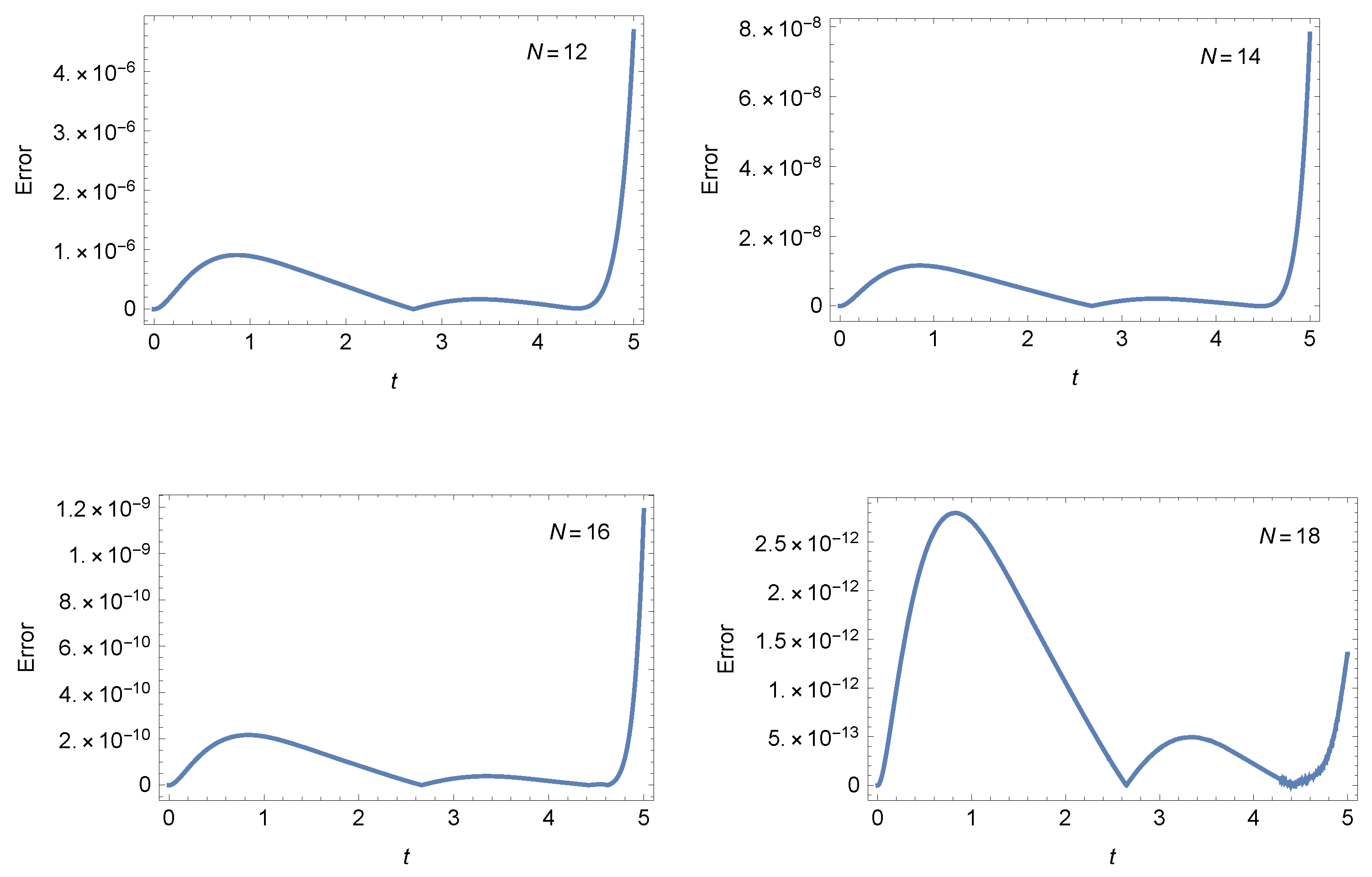
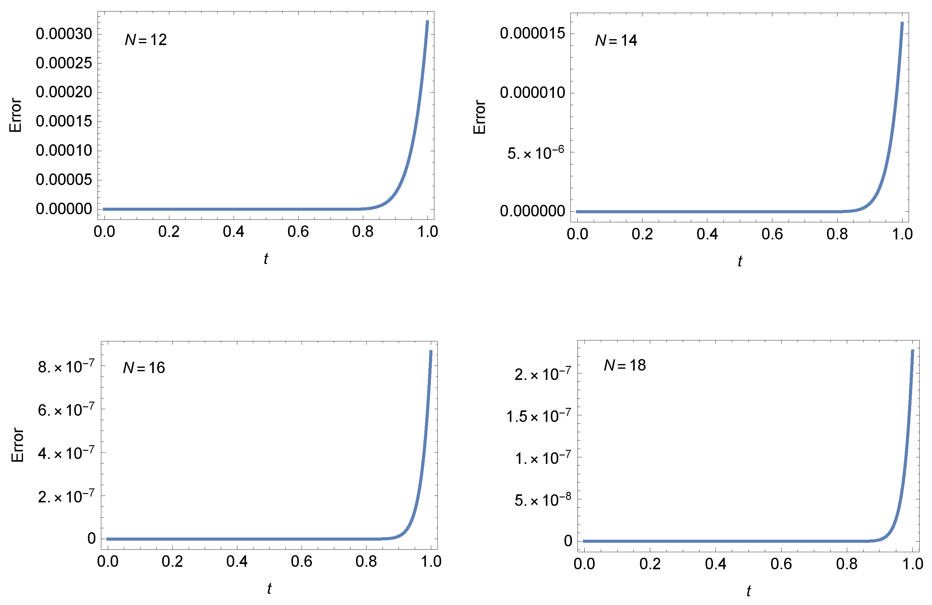
- Case 1: For , Table 4 and Table 5 present the AEs at different values of at, respectively, and when . Table 6 presents the AEs at different values of at when . Figure 4 shows that the approximate solutions have smaller variations for values of α and β near the values and when Table 7 presents the absolute errors (AEs) at different values of at when and .
Table 4. AEs of Example 2 at .
Table 5. AEs of Example 2 at .
Table 6. AEs of Example 2 at .
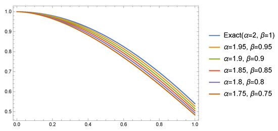 Figure 4. Different solutions of Example 2 at and different values of .
Table 7. AEs of Example 2 at .
Figure 4. Different solutions of Example 2 at and different values of .
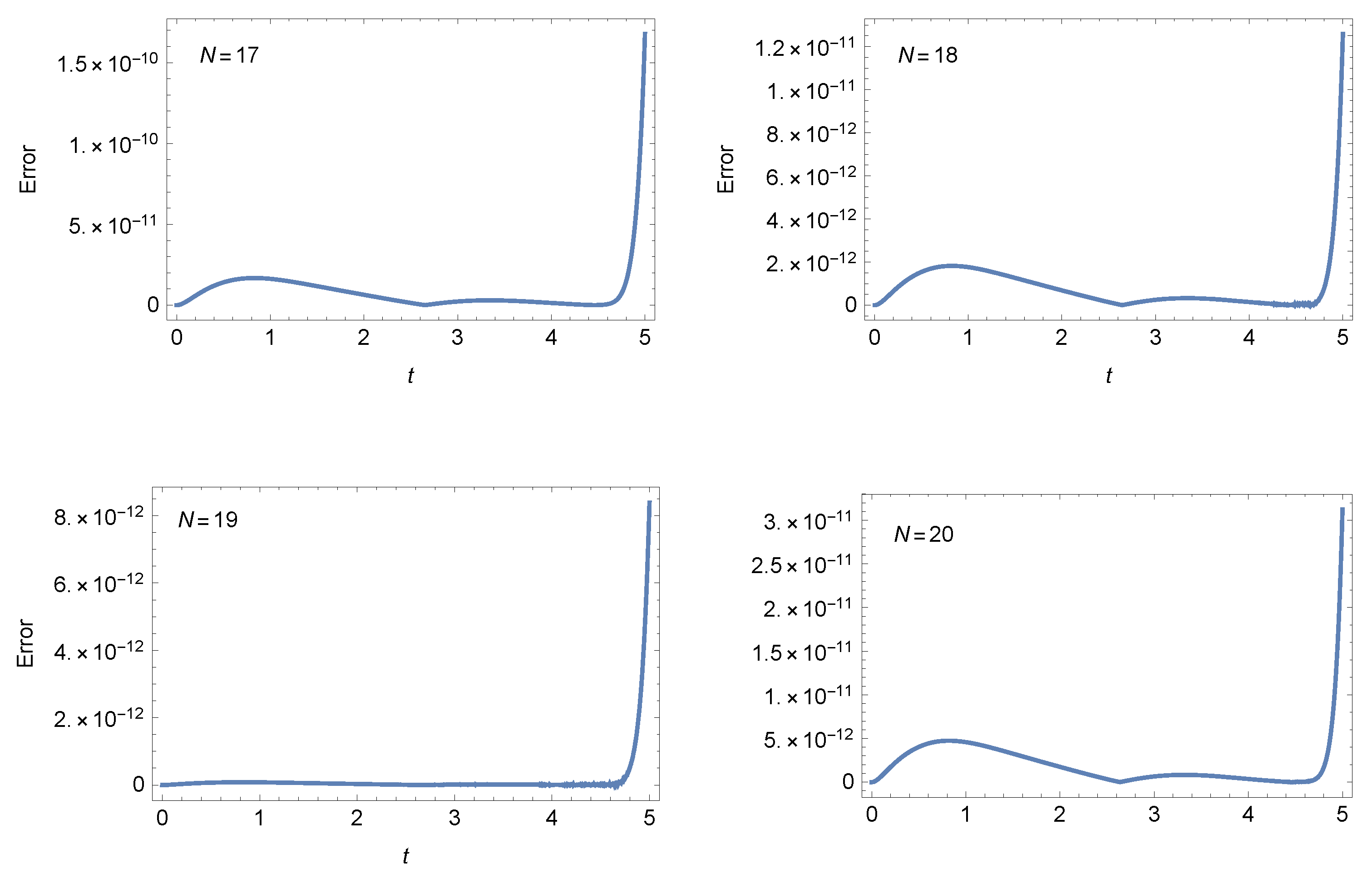
Table 7. AEs of Example 2 at . - Case 2: For and , Figure 5 shows the AEs at different values of N when . Also, Figure 6 illustrates the AEs at different values of N when . These figures show the accuracy of our method.
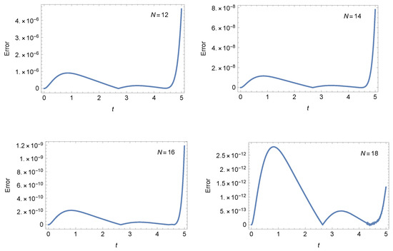 Figure 5. The AEs of Example 2 at .
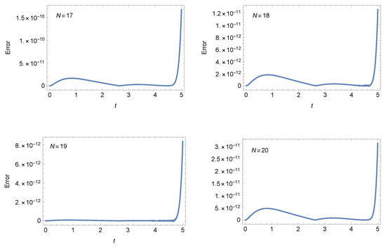 Figure 6. The AEs of Example 2 at .
Remark 7.
The results of Table 4 demonstrate that the small values of N cause clear variation in the error values for different choices of the parameters a and b. For instance, for , the error changes from to at due to the change of the involved parameters. Especially at larger time steps, the error differences brought on by variations in a and b become slightly less obvious.
Example 3.
Consider the following NFDE:
which is governed by
Due to the nonavailability of the exact solution, let us define the following absolute residual error norm at :
and apply our method at when .
Figure 7 illustrates the RE (left) and approximate solution (right) at and . Also, Figure 8 illustrates the RE at different values of N when and
Figure 7.
The RE (left) and approximate solution (right) of Example 3 at and .
Figure 8.
The RE of Example 3 at .
Remark 8.
The numerical results obtained in this section show that we have received several highly accurate approximate solutions using the combined Fibonacci–Lucas polynomials. This gives us an advantage in introducing these generalized polynomials.
Remark 9.
We comment that the approximations resulting from utilizing other generalized polynomials, such as ultraspherical and Jacobi polynomials, do not change significantly due to the change of their parameters, especially for large values of the retained modes; see, for example, [57].
Remark 10.
The combined Fibonacci–Lucas polynomials provide excellent approximations, since an order error is sometimes reached for certain choices of , and N.
Remark 11.
Combining Fibonacci–Lucas polynomials leads to little improvement in numerical results, since the change of the two parameters a and b leads to small changes in the resulting errors.
7. Concluding Remarks
This paper established a generalized sequence of polynomials, namely, unified Fibonacci–Lucas polynomials. The well-known polynomial sequences of Fibonacci and Lucas are particular types of these polynomials. These polynomials have two parameters, yielding various solutions for every choice of them. Some theoretical results concerned with these polynomials were the keys to implementing our numerical algorithms for solving the second-order and the fractional-order Duffing nonlinear DEs via the celebrated collocation method. The operational matrices of derivatives of the Fibonacci–Lucas polynomials that are derived using the derivative formula of these polynomials were employed to design the proposed numerical algorithm. We comment here that For every choice of the two parameters a and b, a numerical solution was obtained. The numerical results show that the change in the absolute errors caused by variations in the two parameters of the combined Fibonacci–Lucas polynomials is minimal when choosing large values of the retained modes; however, these variations become larger for small values of the retained modes. We aim to investigate the impact of these parameters when solving other types of differential equations. We believe that this is the first time these polynomials have been employed in applications. Future research directions may involve employing these polynomials to solve other types of DEs.
Author Contributions
Conceptualization, W.M.A.-E. and A.G.A.; Methodology, W.M.A.-E., O.M.A. and A.G.A.; Software, W.M.A.-E. and A.G.A.; Validation, W.M.A.-E., O.M.A., A.K.A. and A.G.A.; Formal analysis, W.M.A.-E. and A.G.A.; Investigation, W.M.A.-E., O.M.A., A.K.A. and A.G.A.; Writing—original draft, W.M.A.-E. and A.G.A.; Writing—review & editing, W.M.A.-E. and A.G.A.; Supervision, W.M.A.-E.; Funding acquisition, A.K.A. All authors have read and agreed to the published version of the manuscript.
Funding
This research work was funded by Umm Al-Qura University, Saudi Arabia, under grant number 25UQU4331287GSSR03.
Data Availability Statement
The data are contained within the article.
Acknowledgments
The authors extend their appreciation to Umm Al-Qura University, Saudi Arabia, for funding this research work through grant number 25UQU4331287GSSR03.
Conflicts of Interest
The authors declare no conflicts of interest.
References
- Boyd, J.P. Chebyshev and Fourier Spectral Methods; Courier Corporation: North Chelmsford, MA, USA, 2001. [Google Scholar]
- Hesthaven, J.; Gottlieb, S.; Gottlieb, D. Spectral Methods for Time-Dependent Problems; Cambridge University Press: Cambridge, UK, 2007; Volume 21. [Google Scholar]
- Trefethen, L.N. Spectral Methods in MATLAB; SIAM: Philadelphia, PA, USA, 2000; Volume 10. [Google Scholar]
- Koshy, T. Fibonacci and Lucas Numbers with Applications; John Wiley & Sons: Hoboken, NJ, USA, 2019. [Google Scholar]
- Ozkan, E.; Altun, I. Generalized Lucas polynomials and relationships between the Fibonacci polynomials and Lucas polynomials. Comm. Algebra 2019, 47, 4020–4030. [Google Scholar] [CrossRef]
- Özkan, E.; Taştan, M. On Gauss Fibonacci polynomials, on Gauss Lucas polynomials and their applications. Comm. Algebra 2020, 48, 952–960. [Google Scholar] [CrossRef]
- Du, T.; Wu, Z. Some identities involving the bi-periodic Fibonacci and Lucas polynomials. AIMS Math. 2023, 8, 5838–5846. [Google Scholar] [CrossRef]
- Haq, S.; Ali, I. Approximate solution of two-dimensional Sobolev equation using a mixed Lucas and Fibonacci polynomials. Eng. Comput. 2022, 38, 2059–2068. [Google Scholar] [CrossRef]
- Mohamed, A.S. Fibonacci collocation pseudo-spectral method of variable-order space-fractional diffusion equations with error analysis. AIMS Math. 2022, 7, 14323–14337. [Google Scholar] [CrossRef]
- Manohara, G.; Kumbinarasaiah, S. An Innovative Fibonacci Wavelet Collocation Method for the Numerical Approximation of Emden-Fowler Equations. Appl. Numer. Math. 2024, 201, 347–369. [Google Scholar]
- Abd-Elhameed, W.M.; Al-Harbi, A.K.; Alqubori, O.M.; Alharbi, M.H.; Atta, A.G. Collocation method for the time-fractional generalized Kawahara equation using a certain Lucas polynomial sequence. Axioms 2025, 14, 114. [Google Scholar] [CrossRef]
- Abd-Elhameed, W.M. Novel expressions for the derivatives of sixth-kind Chebyshev polynomials: Spectral solution of the non-linear one-dimensional Burgers’ equation. Fractal Fract. 2021, 5, 74. [Google Scholar] [CrossRef]
- Youssri, Y.H.; Abd-Elhameed, W.M.; Abdelhakem, M. A robust spectral treatment of a class of initial value problems using modified Chebyshev polynomials. Math. Methods Appl. Sci. 2021, 44, 9224–9236. [Google Scholar] [CrossRef]
- Ahmed, H.M. A new first finite class of classical orthogonal polynomials operational matrices: An application for solving fractional differential equations. Contemp. Math. 2023, 4, 974–994. [Google Scholar] [CrossRef]
- Tohidi, E.; Bhrawy, A.H.; Erfani, K. A collocation method based on Bernoulli operational matrix for numerical solution of generalized pantograph equation. Appl. Math. Model. 2013, 37, 4283–4294. [Google Scholar] [CrossRef]
- Abd-Elhameed, W.M.; Alsuyuti, M.M. New spectral algorithm for fractional delay pantograph equation using certain orthogonal generalized Chebyshev polynomials. Commun. Nonlinear Sci. Numer. Simul. 2025, 141, 108479. [Google Scholar] [CrossRef]
- Ahmed, H.M. New generalized Jacobi Galerkin operational matrices of derivatives: An algorithm for solving multi-term variable-order time-fractional diffusion-wave equations. Fractal Fract. 2024, 8, 68. [Google Scholar] [CrossRef]
- Enns, R.M. Nonlinear Phenomena in Physics and Biology; Springer Science & Business Media: New York, NY, USA, 2012; Volume 75. [Google Scholar]
- Hilborn, R.C. Chaos and Nonlinear Dynamics: An Introduction for Scientists and Engineers; Oxford University Press: Oxford, UK, 2000. [Google Scholar]
- Magin, R. Fractional calculus in bioengineering, part 1. Crit. Rev. Biomed. Eng. 2004, 32, 1–104. [Google Scholar] [CrossRef]
- Abd-Elhameed, W.M.; Ahmed, H.M. Spectral solutions for the time-fractional heat differential equation through a novel unified sequence of Chebyshev polynomials. AIMS Math. 2024, 9, 2137–2166. [Google Scholar] [CrossRef]
- Wang, F.; Hou, E.; Salama, S.A.; Khater, M.M.A. Numerical investigation of the nonlinear fractional Ostrovsky equation. Fractals 2022, 30, 2240142. [Google Scholar] [CrossRef]
- Amin, A.Z.; Abdelkawy, M.A.; Solouma, E.; Al-Dayel, I. A spectral collocation method for solving the non-linear distributed-order fractional Bagley–Torvik differential equation. Fractal Fract. 2023, 7, 780. [Google Scholar] [CrossRef]
- Heydari, M.H.; Razzaghi, M.; Baleanu, D. A numerical method based on the piecewise Jacobi functions for distributed-order fractional Schrödinger equation. Commun. Nonlinear Sci. Numer. Simul. 2023, 116, 106873. [Google Scholar] [CrossRef]
- Kovacic, I.; Brennan, M.J. The Duffing Equation: Nonlinear Oscillators and Their Behaviour; John Wiley & Sons: Hoboken, NJ, USA, 2011. [Google Scholar]
- Alvarez-Ramirez, J.; Espinosa-Paredes, G.; Puebla, H. Chaos control using small-amplitude damping signals. Phys. Lett. A 2003, 316, 196–205. [Google Scholar] [CrossRef]
- Aghdam, M.M.; Fallah, A. Analytical Solutions for Generalized Duffing Equation. In Nonlinear Approaches in Engineering Applications: Advanced Analysis of Vehicle Related Technologies; Springer: Cham, Switzerland, 2016; pp. 263–278. [Google Scholar]
- El-Sayed, A.A. Pell-Lucas polynomials for numerical treatment of the nonlinear fractional-order Duffing equation. Demonstr. Math. 2023, 56, 20220220. [Google Scholar] [CrossRef]
- Wang, Y.R.; Chen, G.W. Predicting multiple numerical solutions to the Duffing equation using machine learning. Appl. Sci. 2023, 13, 10359. [Google Scholar] [CrossRef]
- Kamiński, M.; Corigliano, A. Numerical solution of the Duffing equation with random coefficients. Meccanica 2015, 50, 1841–1853. [Google Scholar] [CrossRef]
- Elías-Zúñiga, A. A general solution of the Duffing equation. Nonlinear Dynam. 2006, 45, 227–235. [Google Scholar] [CrossRef]
- Abdulganiy, R.I.; Wen, S.; Feng, Y.; Zhang, W.; Tang, N. Adapted block hybrid method for the numerical solution of Duffing equations and related problems. AIMS Math. 2021, 6, 14013–14034. [Google Scholar] [CrossRef]
- Geng, F. Numerical solutions of Duffing equations involving both integral and non-integral forcing terms. Comput. Math. Appl. 2011, 61, 1935–1938. [Google Scholar] [CrossRef]
- Tabatabaei, K.; Gunerhan, E. Numerical solution of Duffing equation by the differential transform method. Appl. Math. Inf. Sci. Lett. 2014, 2, 1–6. [Google Scholar]
- Salas, A.H.; Castillo, J.E. Exact solutions to cubic Duffing equation for a nonlinear electrical circuit. Visión Electrónica 2014, 8, 46–53. [Google Scholar]
- Singh, H.; Srivastava, H.M. Numerical investigation of the fractional-order Liénard and Duffing equations arising in oscillating circuit theory. Front. Phys. 2020, 8, 120. [Google Scholar] [CrossRef]
- Kim, V.A.; Parovik, R.I.; Rakhmonov, Z.R. Implicit finite-difference scheme for a Duffing oscillator with a derivative of variable fractional order of the Riemann-Liouville Type. Mathematics 2023, 11, 558. [Google Scholar] [CrossRef]
- Kim, V.A.; Parovik, R.I. Some aspects of the numerical analysis of a fractional duffing oscillator with a fractional variable order derivative of the Riemann-Liouville type. AIP Conf. Proc. 2022, 2467, 060014. [Google Scholar]
- Canuto, C.; Hussaini, M.Y.; Quarteroni, A.; Zang, T.A. Spectral Methods in Fluid Dynamics; Springer: Berlin/Heidelberg, Germany, 1988. [Google Scholar]
- Alsuyuti, M.M.; Doha, E.H.; Ezz-Eldien, S.S. Galerkin operational approach for multi-dimensions fractional differential equations. Commun. Nonlinear Sci. Numer. Simul. 2022, 114, 106608. [Google Scholar] [CrossRef]
- Atta, A.G.; Abd-Elhameed, W.M.; Moatimid, G.M.; Youssri, Y.H. Shifted fifth-kind Chebyshev Galerkin treatment for linear hyperbolic first-order partial differential equations. Appl. Numer. Math. 2021, 167, 237–256. [Google Scholar] [CrossRef]
- Hafez, R.M.; Youssri, Y.H. Fully Jacobi–Galerkin algorithm for two-dimensional time-dependent PDEs arising in physics. Int. J. Mod. Phys. C 2024, 35, 2450034. [Google Scholar] [CrossRef]
- Atta, A.G.; Abd-Elhameed, W.M.; Moatimid, G.M.; Youssri, Y.H. Modal shifted fifth-kind Chebyshev tau integral approach for solving heat conduction equation. Fractal Fract. 2022, 6, 619. [Google Scholar] [CrossRef]
- El-Sayed, A.A.; Boulaaras, S.; Sweilam, N.H. Numerical solution of the fractional-order logistic equation via the first-kind Dickson polynomials and spectral tau method. Math. Meth. Appl. Sci. 2023, 46, 8004–8017. [Google Scholar] [CrossRef]
- Tu, H.; Wang, Y.; Yang, C.; Liu, W.; Wang, X. A Chebyshev–Tau spectral method for coupled modes of underwater sound propagation in range-dependent ocean environments. Phys. Fluids 2023, 35, 037113. [Google Scholar] [CrossRef]
- Mostafa, D.; Zaky, M.A.; Hafez, R.M.; Hendy, A.S.; Abdelkawy, M.A.; Aldraiweesh, A.A. Tanh Jacobi spectral collocation method for the numerical simulation of nonlinear Schrödinger equations on unbounded domain. Math. Meth. Appl. Sci. 2023, 46, 656–674. [Google Scholar] [CrossRef]
- Weera, W.; Kumar, R.S.V.; Sowmya, G.; Khan, U.; Prasannakumara, B.C.; Mahmoud, E.E.; Yahia, I.S. Convective-radiative thermal investigation of a porous dovetail fin using spectral collocation method. Ain Shams Eng. J. 2023, 14, 101811. [Google Scholar] [CrossRef]
- Atta, A.G. Two spectral Gegenbauer methods for solving linear and nonlinear time fractional Cable problems. Int. J. Mod. Phys. C 2023, 35, 2450070. [Google Scholar] [CrossRef]
- Abd-Elhameed, W.M.; Alqubori, O.M.; Atta, A.G. A collocation procedure for treating the time-fractional FitzHugh–Nagumo differential equation using shifted Lucas polynomials. Mathematics 2024, 12, 3672. [Google Scholar] [CrossRef]
- Abd-Elhameed, W.M.; Alqubori, O.M.; Atta, A.G. A collocation procedure for the numerical treatment of FitzHugh–Nagumo equation using a kind of Chebyshev polynomials. AIMS Math. 2025, 10, 1201–1223. [Google Scholar] [CrossRef]
- Lyapin, A.P.; Akhtamova, S.S. Recurrence relations for the sections of the generating series of the solution to the multidimensional difference equation. Vestnik Udmurtskogo Universiteta Matematika Mekhanika Komp’yuternye Nauki 2021, 31, 414–423. [Google Scholar] [CrossRef]
- Pirmohabbati, P.; Sheikhani, A.H.R.; Najafi, H.S.; Ziabari, A.A. Numerical solution of full fractional Duffing equations with Cubic-Quintic-Heptic nonlinearities. AIMS Math. 2020, 5, 1621–1641. [Google Scholar] [CrossRef]
- Novozhenova, O.G. Life and science of Alexey Gerasimov, one of the pioneers of fractional calculus in Soviet Union. Fract. Calc. Appl. Anal. 2017, 20, 790–809. [Google Scholar] [CrossRef]
- Caputo, M.; Fabrizio, M. On the notion of fractional derivative and applications to the hysteresis phenomena. Meccanica 2017, 52, 3043–3052. [Google Scholar] [CrossRef]
- Caputo, M. Linear models of dissipation whose Q is almost frequency independent—II. Geophys. J. Int. 1967, 13, 529–539. [Google Scholar] [CrossRef]
- Gerasimov, A.N. Generalization of linear deformation laws and their application to internal friction problems. Appl. Math. Mech. 1948, 12, 529–539. [Google Scholar]
- Hafez, R.M.; Zaky, M.A.; Abdelkawy, M.A. Jacobi spectral Galerkin method for distributed-order fractional Rayleigh–Stokes problem for a generalized second grade fluid. Front. Phys. 2020, 7, 240. [Google Scholar] [CrossRef]

Disclaimer/Publisher’s Note: The statements, opinions and data contained in all publications are solely those of the individual author(s) and contributor(s) and not of MDPI and/or the editor(s). MDPI and/or the editor(s) disclaim responsibility for any injury to people or property resulting from any ideas, methods, instructions or products referred to in the content. |
© 2025 by the authors. Licensee MDPI, Basel, Switzerland. This article is an open access article distributed under the terms and conditions of the Creative Commons Attribution (CC BY) license (https://creativecommons.org/licenses/by/4.0/).