Abstract
This paper studies the effects of resource limitations, immunity decay, and delays on an Ebola epidemic model and an optimal control strategy. The model includes two types of delays: a delay in the incubation period of infected individuals and a delay in treatment. Conditions for a Hopf bifurcation at the endemic equilibrium are verified, with its direction and stability analyzed via normal form theory and the center manifold theorem. We also studied the optimal control problem for the SIRD delay model using educational campaigns and Ebola survivors’ immunity as control variables. Furthermore, we formulate an optimization problem based on Pontryagin’s maximum principle. This problem uses a modified Runge-Kutta approach with delays to discover the best control strategy to reduce infections and intervention costs. Finally, simulation results confirm analytical conclusions and show the practical implications of the optimum Ebola control plan using the dde23 MATLAB R2024a built-in solver and DDE-Biftool.
MSC:
34C23; 34D20; 49K40; 49J15; 37M05
1. Introduction
Ebola virus disease was first discovered in 1976, and among infectious diseases, it is one of the most perilous known to humanity. The death rates for people infected with this disease are very high and may reach 90 percent in some cases [1]. The Ebola virus spreads widely among humans in several ways, and infection occurs during the processes of consumption, cooking, or preparation. Individuals may encounter infected animals and come into contact with clothing or items that contain the bodily fluids of an infected person; contact with their urine, feces, semen, or saliva can cause transmission to occur. Ebola enters the body through the liver or when the nose, mouth, or eyes are bitten. In addition, the Ebola virus is also spread to humans by fruit bats, chimpanzees, and monkeys [2,3]. From 2 to 21 days is the range for Ebola’s incubation period, with symptoms such as skin rash, vomiting, diarrhea, and tremors, and severe cases can lead to internal and external bleeding [1,4]. The epidemic had a severe impact on many countries. To curb the rapid spread of the disease, quarantining—a time-tested method—is implemented to isolate those suspected of being infected. Even though it has proved effective in controlling the disease, it also poses significant challenges for public health. Furthermore, direct contact with the deceased during burial ceremonies can facilitate the transmission of the disease [5,6].
The dynamics of Ebola transmission have been extensively studied, revealing insights into the disease’s spread and control. Zoonotic transmission between dogs and humans [7], the progression of the disease through different stages [8], and the impact of density-dependent treatment approaches on Ebola transmission [9] have been explored. A modified mathematical model incorporating quarantining as a control strategy has also been developed [10]. In addition, research has focused on direct and indirect transmission routes; as stated in [11], the models incorporated a composite nonlinear incidence function along with density-independent treatment. The significance of vaccination in reducing mortality among confirmed Ebola patients is highlighted in an observational study [12]. A comprehensive eight-dimensional nonlinear differential equations model is presented to better understand Ebola transmission dynamics [13]. The role of optimal control strategies in human–bat transmission dynamics is also investigated [14]. This study aims to model the dynamics of Ebola by incorporating time delay, immunity, quarantining, and nonlinear perturbations as control mechanisms. The influence of quarantine, medical resource availability, the latent period, and treatment delays were key factors in this study, especially during the early phases of model development. As the research progressed, additional characteristics of Ebola were integrated to enhance the model. The critical roles of quarantine and medical resources, along with the latent period’s significance in Ebola dynamics, are central to this research. This study, inspired by previous research [15], aims to develop computational models focusing on time delays and quarantine for effective Ebola control, particularly in outbreaks like those in Western Guinea. The research also draws inspiration from studies that used modeling methods to understand and mitigate Ebola [16,17].
Delay differential equations (DDEs) offer a more complex dynamic than ordinary differential equations, as the introduction of time delays can destabilize previously stable equilibria, leading to population fluctuations [18,19,20]. This makes the study of delays essential for understanding population dynamics, especially in the context of epidemics, where various infectious diseases exhibit different types of delays during their spread. A comprehensive overview of the relevance of DDEs in population dynamics and epidemics is given in [21]. Various scenarios with the inclusion of delays have been analyzed by researchers, including vaccination periods [22], asymptomatic carriage and infection periods [23], immunity periods, and incubation or latent periods [23,24,25,26]. In [27], the research focuses on an SEIRS model, specifically examining the impact of constant delays on both immune periods and the latent period, and [23] analyzes a model with delays in both asymptomatic carriage period and incubation. In addition, the authors of [28] examined the stability of periodic solutions within a delayed feedback control system and the existence of bifurcation.
Hopf bifurcation in virus infection models with three delays and CTL responses is the focus of study in [29]. A delayed SIQR epidemic model is explored, and different pairs of delays are used as bifurcation parameters in [30]. A delayed SEIS epidemic model, including an analysis of Hopf bifurcation, is explored in [31].
In a more detailed study, the authors of [32] developed a model of the Ebola epidemic that takes into account the loss of immunity, limited medical resources, and the identification and isolation of susceptible individuals. However, their analysis was limited to the disease-free equilibrium, and they did not include time delays or control measures. Our study extends this work by introducing two critical time delays: the incubation period delay and the treatment initiation delay. These delays provide a more realistic representation of disease progression and medical response. In addition, we present two optimal control strategies—quarantine and immune enhancement—allowing us to study their impact on disease control. Furthermore, unlike the original study, we analyze the stability of the endemic equilibrium and explore the conditions under which Hopf bifurcation occurs, leading to periodic outbreaks. This expanded analysis provides deeper insights into disease dynamics and the effectiveness of public health measures.
The inclusion of two time delays, (incubation period delay) and (treatment delay), is of biological and mathematical importance. The incubation delay captures the period between infection and contagion, which affects the early dynamics of the outbreak. The treatment delay represents the delay in medical intervention, which affects recovery rates and disease persistence. Mathematically, these delays act as bifurcation parameters, meaning that if they exceed certain critical thresholds, the system undergoes Hopf bifurcation, leading to persistent oscillations in the spread of the disease. This suggests that reducing treatment delays could be an effective strategy to prevent periodic outbreaks and control an epidemic more efficiently.
The rest of this article is organized as follows: In Section 2, we develop a mathematical model that incorporates multiple time delays, and for the solution, we establish boundedness and positivity. Section 3 presents an analysis of the disease-free equilibrium local stability and derives the conditions necessary for the local stability of the interior equilibrium point. Section 4 provides a comprehensive analysis of Hopf bifurcation, focusing on both the stability characteristics of the resulting periodic solutions and the direction in which the bifurcation occurs. Further, in Section 5, the associated optimal control system’s formulation and solution are detailed. Numerical simulations confirm the theoretical results in Section 6.
2. Formulation of the Model and Analysis of Solution Positivity
Our study is built upon the epidemiological model proposed in [32], which considers the dynamics of infection, recovery, and deceased individuals who are not yet buried. We extend this model by incorporating time delays and control strategies to analyze disease dynamics more comprehensively.
This model employs a framework to classify the population into four categories: susceptible (S), infectious (I), recovered (R), and deceased individuals awaiting burial (D). It also explores the latent period for those exposed to the infection, specifically measuring the time from the initial Ebola virus infection to the appearance of symptoms. This period can be affected by the overall viral transmission rate within the community and the individual’s immune response. It is understood that recovered individuals, labeled as R, gradually lose their immunity over time and reintegrate into the susceptible population. Moreover, in light of the widespread nature of the virus, effective tracing and quarantining of susceptible individuals can play a critical role in controlling the outbreak. This is mainly demonstrated through a decrease in the transmission probability, denoted as u.
In our study, we define (for susceptible individuals) the latent period ; these parameters represent the time intervals that elapse from the moment an individual is infected until they become capable of transmitting the infection, and for the delay in treatment, we denote this as ; this represents when infected individuals do not recover immediately after infection but only after a period of delay due to treatment such as diagnosis and medical intervention.
with the initial conditions
Here, , , with and Further, is described in detail in [33]. In the model equations, the deceased compartment D only accumulates individuals who die due to infection at a rate of . Naturally deceased individuals with a rate of d from the compartments , and R do not enter into D and are directly removed from the system. Furthermore, our model includes time delays, with a particular focus on the disease latent period represented by the parameter and the delay in treatment denoted by , where . The model parameters are defined in Table 1.

Table 1.
Table of parameters used in model (1).
To model the interactions between the four compartments, we propose the following assumptions:
- The variable u ranges from 0 to 1; when , the quarantine measures are ineffective, while indicates that the quarantine is fully enforced;
- Delayed effects: Individuals infected at time become infectious later at time t, so we express their contribution to infectivity as . Likewise, captures the treatment delay from to recovery at time t for infectious individuals.
The disease-free equilibrium (DFE) point of the model (1) is given by , where . A critical parameter, the basic reproduction number (BRN), represented as , often influences the stability of the equilibrium points within the system. This important factor shows how many new infections one sick person can cause while they are contagious in a population where everyone else is at risk of becoming infected.
We determine the basic reproduction number of model (1) for the system using the next-generation matrix [37,38]. It is similar to that used in [32]. However, for the reader’s interest, we provide a sketch of the idea. The disease-free equilibrium (DFE) of the system (1) is given by At the DFE, the matrices and , representing the rate of appearance of new infections and the rate of transfer between compartments, respectively, are defined as follows:
The Jacobian matrices of and at are computed as
The next-generation matrix is given by
By computing the spectral radius of , we obtain
Here, the first term represents the expected number of secondary cases produced by an infected individual in a fully susceptible population, while the second term accounts for the contribution of deceased but not yet buried individuals.
Solution Positivity and Boundedness
We provide the following lemma, which is pertinent to this field, to prove the positivity and eventual boundedness of the solutions , , , and of model (1).
Lemma 1.
Moreover, if holds for , then
Proof.
From (2), it is clear that . Suppose we assume that there exists such that for any . Further, assume that and for any .
From the first equation of (1), we obtain This contradicts the fact that and for . Now, from the remaining equations of (1), we obtain
From the above equations and the fact that , we have and for some This proves (3).
Based on the discussion above and the use of the comparison principle, as a result, . □
3. Stability Analysis
This section focuses on the examination of the stability characteristics of the equilibrium points in system (1). First, we present the results concerning the local asymptotic stability of .
3.1. Local Stability of Disease-Free Equilibrium
The (DFE) of model (1) is given by . The Jacobian matrix at is represented by
where . The system’s characteristic equation is expressed as follows:
Appendix A outlines the specific forms of , , and for . Given the two different delays of and , we state the following theorems:
Theorem 1.
The is locally asymptotically stable for if .
Proof.
If , this means the system is without time delay. For the proof, refer to Theorem 2 in [32]. □
Theorem 2.
Suppose (A5) has a positive root; then, the is locally asymptotically stable for with .
Theorem 3.
Suppose (A9) has a positive root; then, the is locally asymptotically stable for , with .
Theorem 4.
Suppose (A13) has a positive root; then, the is locally asymptotically stable for , , where .
Remark 1.
For details on the proofs of Theorems 2–4, please refer to Appendix C.
3.2. Stability Analysis of Interior Equilibria and Hopf Bifurcation
If , the system described by (1) demonstrates the presence of a unique endemic equilibrium, denoted by . By using the same method as in [32], we find
The Jacobian matrix at the equilibrium point can be written in the following form:
where
At the endemic equilibrium , the characteristic equation of the linearized model system (1) is
where the expressions for , , and , , are given in Appendix B.
Theorem 5.
If and , then the endemic point for is locally asymptotically stable.
For different delays of and , we have the following theorems:
Theorem 6.
Suppose ; it can be concluded that for all , the endemic equilibrium of system (1) remains locally asymptotically stable.
Theorem 7.
Suppose , and the conditions and (see Appendix C) hold. Then, system (1) undergoes a Hopf bifurcation near , leading to the emergence of a family of periodic solutions from . Furthermore, for with , the endemic equilibrium remains locally asymptotically stable.
Theorem 8.
Suppose , and the conditions and (see Appendix C) hold. Then, system (1) experiences a Hopf bifurcation near the endemic equilibrium , leading to the emergence of a family of periodic solutions from . If , the equilibrium remains locally asymptotically stable.
Remark 2.
Appendix C provides the proofs of Theorems 5–8.
4. Hopf Bifurcation: Direction and Stability
In this section, we investigate the direction of the Hopf bifurcation and the stability of the bifurcating periodic solutions of system (1) with We analyze the properties of Hopf bifurcation at the critical value using the center manifold theorem and the normal form theory [39]. We show that for any one of the critical values, by Suppose and
Given , with , define and .
Thus, serves as the Hopf bifurcation parameter. As a result, we work within the fixed phase space , which does not depend on the delay . Within space C, system (8) is reformulated into a functional differential equation as
where and with
and
where . There is a function with bounded variation for , according to the Riesz representation theorem, such that
Actually, we may have
with being the Dirac delta function. For , we define
and
Consider the bilinear
Given that and are adjoint operators, the eigenvectors of A and corresponding to and , respectively, are and . In this context, . In light of the established definitions of the function and the operator , it becomes evident that we can express the following relationship in a more generalized form:
For , we obtain
The eigenvector of corresponding to can be similarly obtained, where
Therefore, we can choose D as
such that . Assume is the solution to (11) under the specific condition where the parameter is set to zero. Now, we define
On the center manifold , we have , and
We concentrate on the real solution of (11), assuming that M remains real if is real. The local coordinates for the center manifold in the directions of and are denoted by z and . With , we obtain
We write the equation as , where
From Equation (13), we have and , , and ; then,
Notice that on the center manifold close to the origin,
Therefore, we obtain
From system (20), for ,
Noticing , we have
where a constant vector in is defined as . A similar result can be obtained:
In the following, we determine and . By using the definition of A and (25), we obtain
where . From (20) and (23), we have
The coefficients of and in are given, respectively, as follows, where and :
By inserting (29) and (33) into (31) and observing that
and
we finally have
which leads to , where
where
It follows that
Therefore, we obtain
where
The main result is deduced based on the conclusion of Hassard et al. [39]. The stability of the bifurcating periodic solution is influenced by : the solution will be stable (unstable) if (). determines the direction of the Hopf bifurcation; if (), the Hopf bifurcation is supercritical (subcritical). Finally, determines the period of the bifurcating periodic solution, which increases (decreases) if ().
5. Delay Model: Optimal Control
The subsequent section explores the optimal control problem associated with model (1). We delve into the existence and characterization of the problem.
5.1. Formulation
Based on the delay model outlined in Equation (1), we have formulated an optimal control problem that focuses on two main strategies. Let us first introduce the control set of Lebesgue square integrable functions over time .
where is the control variable with and as the minimum and the maximum values of the control variables. The first strategy aims to increase the quarantine rate of susceptible individuals through targeted education campaigns. The second strategy seeks to enhance the immunity of Ebola survivors through a comprehensive approach, which includes nutritional support, regular medical follow-ups, physical and mental rehabilitation, and the prevention of secondary infections. Additionally, the plan emphasizes the importance of adequate rest, stress management, and participation in support groups or clinical trials as vital components for recovery and long-term health.
To implement these strategies, the model is modified by introducing the control variable in place of the parameter u, which governs the quarantine rate. In a similar manner, the parameter , related to immunity enhancement, is replaced by the control variable . Then, the delay model can be expressed in the following manner for the control problem:
This section focuses on managing the movement of individuals into quarantine and achieving permanent immunity, either through natural recovery or full vaccination. Our primary objective is to determine the optimal rate at which individuals should enter quarantine areas and the necessary density for an effective response during health crises. To achieve this, we propose educational programs that raise public awareness about disease transmission, emphasizing the importance of following health precautions. This approach not only promotes responsible behavior but also helps minimize implementation costs.
We assume the population dynamics to be proportional to the infectious, recovered, and deceased (but not yet buried) populations, scaled by factors , , and , respectively. The losses due to control measures are modeled as being proportional to the square of the control intensity, with scaling factors and . The objective function is given as follows. We introduce control variables , which are designed to balance awareness and control measures, allowing for an effective response to public health emergencies while minimizing disruptions to daily life.
Here, the non-negative weight coefficient is (where ). Our goal is to identify an optimal set of variables represented as such that
where the optimal set U is defined as follows:
where is Lebesgue measurable.
5.2. Existence and Characterization
In this part of our study, we focus on finding out if there is a best way to control a given system within a limited time frame. Specifically, we look at the system described by the Equations (37)–(40). Our goal is to determine if an optimal set of control strategies exists that can effectively manage the system’s behavior over this period.
Theorem 9.
Proof.
To show the existence of the control variables, the objective function satisfies the following properties:
- (i)
- The set of control variables and state variables is non-empty. This is derived from the property that the nonlinear functions in Equation (37) exhibit uniform Lipschitz continuity.
- (ii)
- The space of the control variables is closed and convex. Since the function space is known to be closed and convex, this property is satisfied.
- (iii)
- The right-hand side (RHS) of the control model in Equation (37) is bounded. The boundedness of both the state and control variables ensures this condition.
- (iv)
- The objective function is convex with respect to the control variables for . Let with . From Equation (39), we have
This proves the convexity of the objective function.
- (v)
- There exist positive constants and such that
From Equation (39), we can observe that
Thus, the existence and uniqueness of the optimal control variables are established using the Filippov-type lemma [40]. □
As described in [41], the optimal control is characterized by the application of Pontryagin’s maximum principle and the formulation of the Hamiltonian function H, considering a delay in the state.
Theorem 10.
Let the optimal control variables be and , and let the optimal state variables , and be related to the control system (37); then, there exists an adjoint variable
that satisfies the criteria established by the adjoint equations:
For the transversality condition
holds. Furthermore, we present the corresponding optimal controls below:
Proof.
The Hamiltonian is defined as
We define the characteristic function as follows:
As a result of Pontryagin’s maximum principle, adjoint variables (for ) exist and satisfy the following canonical equations:
We impose (43) and manipulate the above inequalities by including the derivatives of the respective variables; additional understanding can be gained through adjoint Equation (42). We obtain the following from deriving the optimality condition:
Thus, we have
From the corresponding optimal controls in (44), if the values of are greater than 1, we consider them as 1; if they are negative, we treat them as 0. This completes the proof. □
6. Numerical Simulations
In this section, we employ numerical simulations to illustrate our theoretical findings using the dde23 MATLAB built-in solver and DDE-Biftool [42], a MATLAB package for numerical continuation and bifurcation analysis of delay differential equations (DDEs). The manual for the latest version of DDE-Biftool is available in [43].
System (49) has a unique endemic equilibrium as for the parametric values provided in Table 1. By using the above-mentioned Matlab tool, the unique endemic equilibrium is determined to be = (10.1495, 105.157, 350.815, 6845.02), which for is locally asymptotically stable (refer to Figure 1).
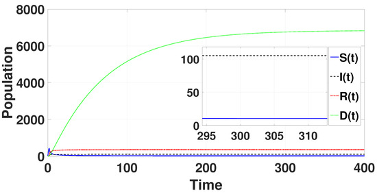
Figure 1.
The endemic equilibrium is shown to be stable through the solution curves of system (49) with .
In Figure 2, the solution curves are presented. Theorem 6 confirms that no Hopf bifurcation occurs in system (49). For , and ; furthermore, according to (A21), we find where ; then, point remains locally asymptotically stable for all with

Figure 2.
The endemic equilibrium is shown to be stable through the solution curves of system (49), with no destabilizing effect of the delay parameter for all and .
Now, for and , we find and . Additionally, we have . Thus, we can conclude that the equilibrium point is locally asymptotically stable when conditions and (see Appendix C) are satisfied for . However, as approaches , will switch stability, becoming unstable and undergoing a Hopf bifurcation at . This transition leads to the emergence of a family of periodic solutions bifurcating from near .
By using DDE-Biftool, we find that when , there are four critical delays: (see Figure 3). Notice that the stability switches occur at the Hopf bifurcation points, leading to a total of seven stability switches. The stable and unstable regions of the branch are represented in green and red, respectively. The branch of periodic solutions emerges from the first critical delay at the Hopf bifurcation point (see Figure 3b). This behavior is further illustrated by the bifurcation diagram in Figure 4, with additional solution curves shown in Figure 5 and Figure 6.
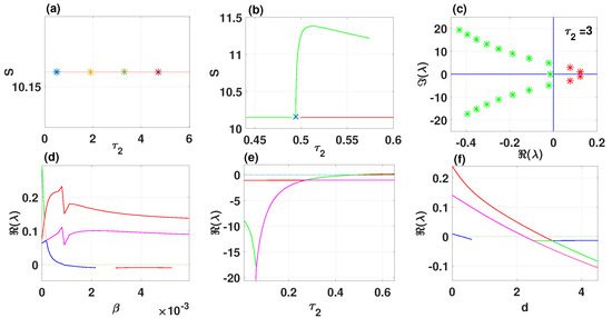
Figure 3.
The endemic equilibrium branch with stability information (a). Plot of the branch of periodic solutions from the first bifurcation point (b). Eigenvalues endemic branch with (c). (d–f) Real parts of eigenvalues vs. , and d, respectively.
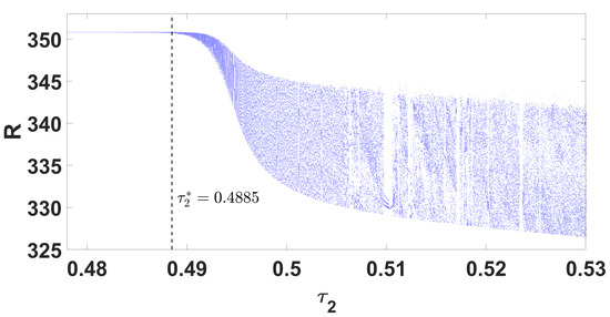
Figure 4.
Parameter bifurcation diagram R with respect to .
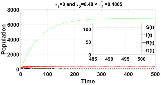
Figure 5.
For the delayed case and , the time series solution of system (49) demonstrates that the endemic equilibrium remains consistently stable for .
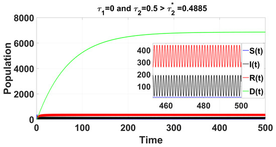
Figure 6.
For the delayed case and , the time series solution of system (49) reveals that the endemic equilibrium becomes unstable for .
Through theoretical analysis, we have determined . Meanwhile, when using DDE-Biftool, the first critical delay is . This indicates that our theoretical result is very close to the outcome obtained from DDE-Biftool. The Figure 7 illustrates the projection of the solutions in the phase space influenced by the delay.
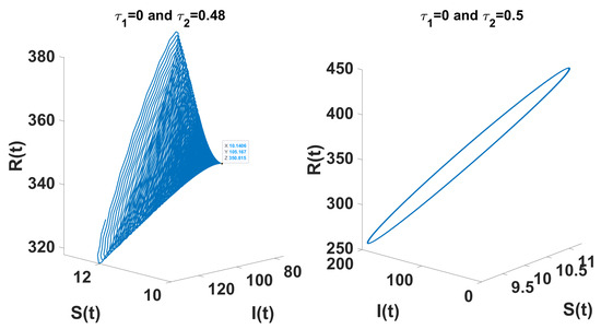
Figure 7.
The left figure shows the system converging to the unique endemic equilibrium for and , while the right figure illustrates convergence to a limit cycle for and .
Through complex computations, we find that and (see Appendix C) are satisfied when . This leads to the following results: , , , and . From Equation (36) in Section 4, we determine that , , , and . As illustrated by the computer simulations (see Figure 8), the positive equilibrium is asymptotically stable when . Once exceeds the critical value , a Hopf bifurcation occurs, causing to lose stability, giving rise to a family of periodic solutions that bifurcate from .
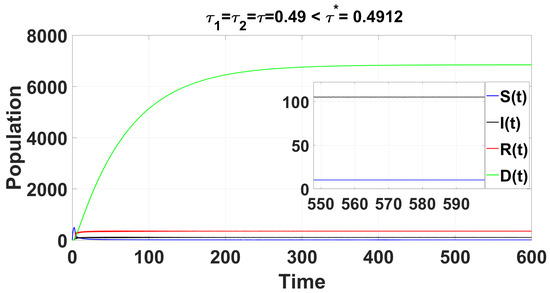
Figure 8.
For the delayed scenario , the time series solution of the system (49) confirms that the endemic equilibrium is stable when .
When using DDE-Biftool with , four critical delays are identified: (see Figure 9). Notably, stability switches occur at the Hopf bifurcation points, resulting in a total of seven stability switches. The stable and unstable portions of the branch are represented in green and red, respectively. The branch of periodic solutions emanates from the first critical time delay at the Hopf bifurcation point (see Figure 9). It is important to note that through our theoretical analysis, we find , whereas when using DDE-Biftool, the first critical delay is . This indicates that our theoretical result is very close to the outcome from DDE-Biftool.
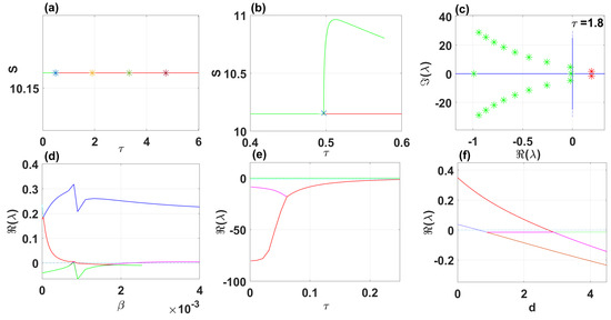
Figure 9.
The endemic equilibrium branch with stability information (a). Plot of the branch of periodic solutions from the first bifurcation point . (b). Eigenvalues endemic branch with (c). (d–f) Real parts of eigenvalues vs. , and d, respectively.
The conditions and indicate a supercritical Hopf bifurcation, with bifurcation occurring for . The periodic solutions bifurcating from at are stable, as depicted in Figure 10; system (49) also undergoes a Hopf bifurcation near , which is demonstrated in the bifurcation diagram (Figure 9b and Figure 11). The right side of Figure 12 denotes the projection of the solutions in .
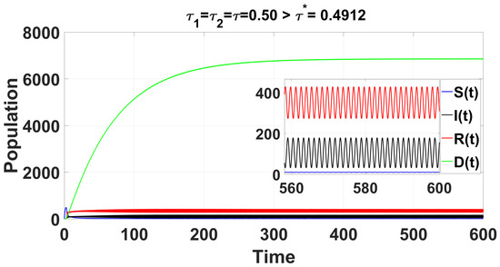
Figure 10.
For the delayed cases when , the time series solution of the system (49) shows that the endemic equilibrium becomes unstable.
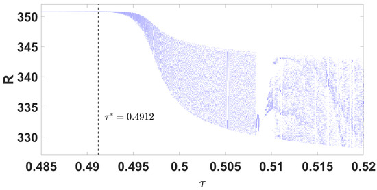
Figure 11.
Parameter bifurcation diagram R with respect to .
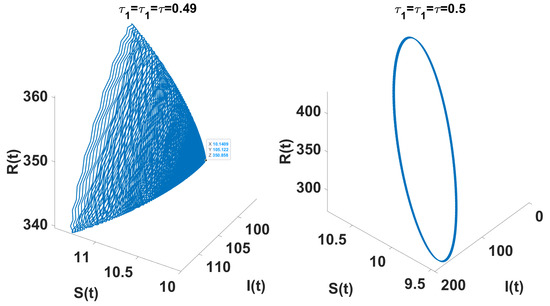
Figure 12.
The left figure shows the system converging to the unique endemic equilibrium for , and the right figure illustrates convergence to a limit cycle for .
Figure 13 shows eigenvalues of the disease-free branch with (a). (b) and (c) show the real parts of eigenvalues vs. and , respectively.
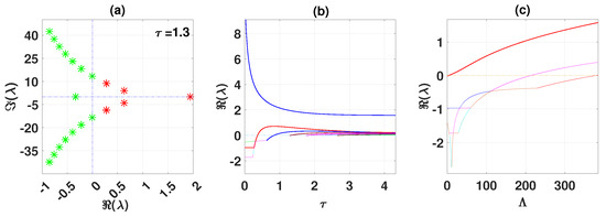
Figure 13.
Eigenvalues disease-free branch with (a). (b,c) Real parts of eigenvalues vs. and , respectively.
Optimal Control Strategies: Numerical Analysis
This section examines the best control strategy using a numerical example for the model. We analyzed the results to better understand how different strategies can impact the spread of the disease. The initial population distribution is given by . From the adjoint and state equations, we first derive the optimality system and, subsequently, solve pandemic model (1) with time delay, control system (37), adjoint Equation (42), the initial conditions (2), and the transversality conditions (43); simulations were carried out using a numerical method derived from the standard Runge-Kutta.
The dynamics of an infected human population can be analyzed by comparing scenarios with and without control interventions. In the given analysis, we refer to the specific parameter values outlined in Table 2, which provide a basis for understanding the effectiveness of these interventions.
Table 2.
Assigned numerical values for the parameters of model (1).
As illustrated in Figure 14, Figure 15 and Figure 16, the model depicts two distinct scenarios: the solid lines represent the population without any form of control, and the dashed lines signify the population under implemented control measures. The weights assigned in the objective function are , , , , and , and these are essential for determining the priorities of different control strategies, influencing the model’s outcomes.
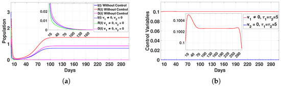
Figure 14.
Plot (a) represents the effect of the control variable on the population over time , and plot (b) illustrates the trajectory of the control variables for and with a delay time of .
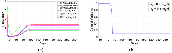
Figure 15.
Plot (a) represents the effect of the control variable on the population over time , and plot (b) illustrates the trajectory of the control variables for and with a delay time of .
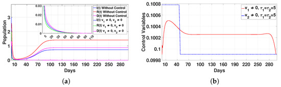
Figure 16.
Plot (a) represents the effect of the control variable on the population over time , and plot (b) illustrates the trajectory of the control variables for and with a delay time of .
The numerical simulations of the SIRD model investigated the impact of two control strategies, efficiency of quarantine protocols () and immunity enhancement (), on achieving a (DFE) . Each control strategy was tested individually and in combination, revealing both their strengths and limitations.
- Case 1: Quarantine protocols only ()In this case, the populations of infected individuals (I), recovered individuals (R), and deceased individuals (D) dropped to zero after 160 days, as shown in Figure 14a. The control was applied at the maximum level for 15 days. After that, we gradually reduced the control application until it was maintained for 70 days at a decreased level. We continued to apply the control at this consistent level for a total of 280 days, after which we significantly decreased the application by 295 days. This approach was effective in reducing disease transmission, but it required long-term implementation, which may be resource-intensive.
- Case 2: Immunity enhancement only ()In this scenario, the infected (I) and deceased (D) populations increase slightly, and the recovered individuals (R) decrease, as shown in Figure 15a. The control is applied at its maximum level for 50 days, and then it drops sharply until day 60, after which it remains stable, as shown in Figure 15b. This strategy alone is not sufficient to eliminate the disease, so we conclude that applying this control by itself is ineffective.
- Case 3: Combined control strategy ()The combined application of two controls yielded the most efficient results. Populations (I), (R), and (D) dropped to zero after 95 days, as presented in Figure 16a. The controls were applied for 20 days () and 50 days (), as displayed in Figure 16b. This integrated approach addressed multiple aspects of disease dynamics simultaneously, achieving faster and more sustainable results than any single intervention.
Each strategy has its advantages and disadvantages. Quarantine protocols () are effective at reducing transmission but require sustained effort, resources, and time. Immunity enhancement () does not prevent new infections and is insufficient to achieve a disease-free state. The combined strategy, while highly effective, may require significant coordination and investment. These findings are crucial for public health planning. They demonstrate that while individual controls can lead to disease-free outcomes, a combined approach is the most robust and efficient. By implementing these strategies, communities can enhance their resilience to outbreaks, save lives, and promote long-term public health stability.
7. Discussion
In this work, we propose a delayed model system that highlights three key concepts: (i) the inclusion of a separate compartment for dead but not yet buried individuals, (ii) the loss of immunity, and (iii) the introduction of a treatment recovery function, , which measures the impact of limited medical resources. The influence of hospital beds and vaccines on disease dynamics was recently detailed by Wang et al. [32], and numerous mathematical models in epidemiology have thoroughly explored the issue of whether recovered individuals have temporary or permanent immunity [45,46]. The results obtained in this paper complement the research work in the literature [32]; our study extends the work of Wang et al. [32] by examining how delay parameters influence system dynamics. Consequently, our proposed model system (1) is made more realistic, particularly when considering diseases like Ebola; after a period of immunity, a recovered person can become susceptible again, as their immunity may only be temporary. We incorporated two time delays into the proposed epidemic model: the latent period for susceptible individuals and treatment delay (due to limited medical resources, also known as the treatment period).
The analysis covers optimal control strategies and explores the model’s solution positivity, boundedness, stability, and Hopf bifurcation to understand better how to manage the system. Additionally, this study investigates the effect of time delay parameters on the dynamics of the model system. The significance of quarantine and boosting immunity in controlling the spread of infection is proven. This paper highlights the importance of quarantine and enhanced immunity in managing an infected population. The primary focus is to examine how the delay parameter influences the system dynamics. Additionally, we explore strategies to enhance quarantine measures, improve disease tracking, and boost immunity levels. Quarantine programs, in particular, are essential for safeguarding individuals and curbing the spread of infectious diseases. This is especially evident in the case of Ebola, where quarantine plays a critical role, underscoring the importance of public awareness regarding seasonal quarantine practices.
Additionally, we found that the combined application of both controls yielded the most efficient results, achieving a disease-free state within 95 days, whereas applying only quarantine protocols took 160 days to reach the same outcome. For various ranges of delay parameters ( and ), the sufficient conditions for local stability of the DFE are explored in Theorems 2–4. The existence of the endemic equilibrium, which is valid when , is directly derived from [32]. We have used the comparison theorem to establish solution boundedness and applied the elementary theory of functional differential equations to ensure the existence and uniqueness of solutions for the proposed model system. Moreover, local stability conditions for the endemic equilibrium are discussed regarding different delay parameter values. In Theorems 7–8, the critical values of both time delays are determined, and the occurrence of Hopf bifurcations is analyzed by treating the delays as bifurcation parameters. Our analysis shows that if the values of time delay and the parameters for system (1) are below their corresponding critical values, the endemic equilibrium remains stable. However, if any delay parameters exceed their critical values, the stability of the endemic equilibrium is lost. One-parameter bifurcation diagrams for different bifurcation parameters are presented in Figure 4 and Figure 11, and the threshold values of the delay parameters are calculated. We used DDE-Biftool to analyze the endemic equilibrium branch and plot the branch of periodic solutions originating from the first bifurcation point, , with . Additionally, we examined the eigenvalues along the endemic equilibrium branch for and , as well as for . We also plotted the real parts of the eigenvalues with respect to , (with ), and d, respectively. See Figure 3 and Figure 9. We used the same tool to plot the eigenvalues along the disease-free equilibrium branch for . Additionally, we plotted the real parts of the eigenvalues as functions of and , respectively.
The study of Hopf bifurcation properties, such as direction and stability, uses a center manifold and normal form theory. The parametric values in (49) corresponding to the endemic equilibrium, where , are discussed. For stability results related to various delay parameters, see Figure 1, Figure 2, Figure 3, Figure 4, Figure 5 and Figure 6, Figure 8, and Figure 10. Our study builds on the work of [32] by incorporating public immunity to evaluate its impact on disease control. It also extends this model by introducing incubation and treatment period delays to analyze their effects on hospital resources and recovery rates. Additionally, we explore strategies to enhance quarantine measures, improve disease tracking, and boost immunity levels. Quarantine programs, in particular, are essential for safeguarding individuals and curbing the spread of infectious diseases. This is especially evident in the case of Ebola, where quarantine plays a critical role, underscoring the importance of public awareness regarding seasonal quarantine practices.
Author Contributions
Conceptualization, H.I., A.H.M. and M.Z.M.; Methodology, H.I. and L.S.; Software, A.H.M.; Validation, S.B.; Formal analysis, H.I. and S.B.; Resources, L.S. and M.Z.M.; Writing—original draft, H.I., A.H.M., S.B. and M.Z.M.; Writing—review & editing, L.S., A.H.M., S.B. and M.Z.M.; Supervision, L.S. All authors have read and agreed to the published version of the manuscript.
Funding
This research was funded by the Deanship of Graduate Studies and Scientific Research, Jazan University, Saudi Arabia (RG24-S066).
Data Availability Statement
Data are contained within the article.
Acknowledgments
The authors gratefully acknowledge the funding of the Deanship of Graduate Studies and Scientific Research, Jazan University, Saudi Arabia, through Project Number: RG24-S066.
Conflicts of Interest
The authors have no conflicts of interest to declare.
Appendix A
Appendix B
Appendix C
Proof of Theorem 2.
Squaring and combining the two equations of (A2) leads to
Now, (A5) possessing a positive root implies that (A4) will have a positive root . Now, from (A2), we have
□
Proof of Theorem 3.
Squaring and combining the two equations of (A7) leads to
□
Proof of Theorem 4.
Given that (A13) has a positive root , then (A12) will have a positive root . From (A11), we now have
□
Proof of the Theorem 5.
Since, for when and . Therefore, the Routh-Hurwitz criterion is satisfied [47]. Consequently, the positive equilibrium is locally asymptotically stable when and are both zero.
□
Proof of the Theorem 6.
If we let (with ) in (A15) and we separate the real and imaginary components, we obtain
with
which implies
where
Let . Then, (A19) becomes
where Since f10 is strictly greater than zero, all the conditions (a)–(c) of Lemma 2.3 in [48] are not satisfied. Thus, all the roots of (A21) will have negative real parts, implying that the system is locally asymptotically stable for all and . Furthermore, we also confirm that conditions (a)–(c) do not hold for our chosen numerical values. □
Proof of the Theorem 7.
Let . Then, Equation (A24) becomes
Under the assumption : If the positive root exists for (A26), then (A24) results in a positive root , and furthermore, we have
Additionally, it can be proven that if the condition
is satisfied, where . Hence, based on the Hopf bifurcation theorem in [49], we conclude Theorem 7 when the conditions and are met. □
Proof of Theorem 8.
This implies
where
Let . Then, (A29) becomes
Consider : Suppose (A31) yields a positive root ; then, Equation (A24) produces a positive root , and furthermore, we find
Furthermore, it can be established that .
is satisfied, where . A is a result, referring to the Hopf bifurcation Theorem [49]; Theorem 8 follows if the conditions and are fulfilled. □
Next, we show that
This implies that for , there is at least one eigenvalue with a positive real part. To find this, we differentiate (A27) with respect to and obtain
Therefore
According to Rouché’s Theorem (see [50]), the root of the characteristic Equation (A27) crosses the imaginary axis from left to right as changes continuously from smaller than to greater than . Therefore, the transversality condition is fulfilled, and the conditions for Hopf bifurcation [51] are met at .
Remark A1.
It is important to emphasize that Theorem 8 cannot establish the stability or direction of the bifurcating periodic solutions. This implies that periodic solutions might exist for close to . To explore the stability of these bifurcating periodic solutions, higher-order terms can be analyzed following the approach of Hassard et al. [39].
References
- World Health Organization. WHO Ebola Situation Reports: Democratic Republic of the Congo. 2023. Available online: https://www.who.int/news-room/fact-sheets/detail/ebola-virus-disease (accessed on 20 April 2023).
- Agusto, F.B.; Teboh-Ewungkem, M.I.; Gumel, A.B. Mathematical assessment of the effect of traditional beliefs and customs on the transmission dynamics of the 2014 Ebola outbreaks. BMC Med. 2015, 13, 96. [Google Scholar] [CrossRef]
- Barbarossa, M.V.; Dénes, A.; Kiss, G.; Nakata, Y.; Röst, G.; Vizi, Z. Transmission dynamics and final epidemic size of Ebola virus disease outbreaks with varying interventions. PLoS ONE 2015, 10, e0131398. [Google Scholar] [CrossRef] [PubMed]
- World Health Organization. WHO Ebola Virus Disease. 2018. Available online: http://www.who.int/mediacentre/factsheets/fs103/en/ (accessed on 8 April 2018).
- Campbell, L.; Adan, C.; Morgado, M. Learning from the Ebola Response in Cities: Responding in the Context of Quarantine. ALNAP. 2017. Available online: https://alnap.org/help-library/resources/learning-from-the-ebola-response-in-cities-responding-in-the-context-of-urban/ (accessed on 25 January 2025).
- Drazen, J.M.; Kanapathipillai, R.; Campion, E.W.; Rubin, E.J.; Hammer, S.M.; Morrissey, S.; Baden, L.R. Ebola Quarantine. N. Engl. J. Med. 2014, 371, 2029–2030. [Google Scholar] [CrossRef]
- Adu, I.K.; Wireko, F.A.; El-N. Osman, M.A.R.; Asamoah, J.K.K. A fractional order Ebola transmission model for dogs and humans. Sci. Afr. 2024, 24, e02230. [Google Scholar] [CrossRef]
- Islam, M.R.; Mahmud, F.; Akbar, M.A. Insights into the Ebola epidemic model and vaccination strategies: An analytical approximate approach. Partial Differ. Equ. Appl. Math. 2024, 11, 100799. [Google Scholar] [CrossRef]
- Kengne, J.N.; Tadmon, C. Ebola virus disease model with a nonlinear incidence rate and density-dependent treatment. Infect. Dis. Model. 2024, 9, 775–804. [Google Scholar] [CrossRef]
- Abbas, N.; Zanib, S.A.; Ramzan, S.; Nazir, A.; Shatanawi, W. A conformable mathematical model of Ebola Virus Disease and its stability analysis. Heliyon 2024, 10, e35818. [Google Scholar] [CrossRef]
- Tadmon, C.; Ndé Kengne, J. Enriched spatiotemporal dynamics of a model of Ebola transmission with a composite incidence function and density-independent treatment. Nonlinear Anal. Real World Appl. 2024, 79, 104118. [Google Scholar] [CrossRef]
- Coulborn, R.M.; Bastard, M.; Peyraud, N.; Gignoux, E.; Luquero, F.; Guai, B.; Mustafa, S.H.; Musenga, E.M.; Ahuka-Mundeke, S. Case fatality risk among individuals vaccinated with rVSVΔG-ZEBOV-GP: A retrospective cohort analysis of patients with confirmed Ebola virus disease in the Democratic Republic of the Congo. Lancet Infect. Dis. 2024, 24, 602–610. [Google Scholar] [CrossRef]
- Ndaïrou, F.; Khalighi, M.; Lahti, L. Ebola epidemic model with dynamic population and memory. Chaos Solitons Fractals 2023, 170, 113361. [Google Scholar] [CrossRef]
- Agbomola, J.O.; Loyinmi, A.C. Modelling the impact of some control strategies on the transmission dynamics of Ebola virus in human-bat population: An optimal control analysis. Heliyon 2022, 8, e12121. [Google Scholar] [CrossRef] [PubMed]
- World Health Organization. WHO Ebola Data and Statistics. 2018. Available online: http://apps.who.int/gho/data/node.ebola-sitrep (accessed on 13 April 2018).
- Legrand, J.; Grais, R.F.; Boelle, P.Y.; Valleron, A.J.; Flahault, A. Understanding the Dynamics of Ebola Epidemics. Epidemiol. Infect. 2007, 135, 610–621. [Google Scholar] [CrossRef] [PubMed]
- Dénes, A.; Gumel, A.B. Modeling the impact of quarantine during an outbreak of Ebola virus disease. Infect. Dis. Model. 2019, 4, 12–27. [Google Scholar] [CrossRef]
- Gopalsamy, K. Stability and Oscillations in Delay Differential Equations of Population Dynamics; Springer: Dordrecht, The Netherlands, 2013; Available online: https://link.springer.com/book/10.1007/978-94-015-7920-9 (accessed on 20 January 2025).
- Zhang, X.; Zhu, H. Hopf bifurcation and chaos of a delayed finance system. Complexity 2019, 2019, 6715036. [Google Scholar] [CrossRef]
- Zhang, Z.; Upadhyay, R.K.; Agrawal, R.; Datta, J. The gestation delay: A factor causing complex dynamics in Gause-type competition models. Complexity 2018, 2018, 1589310. [Google Scholar] [CrossRef]
- Kuang, Y. Delay Differential Equations: With Applications in Population Dynamics; Academic Press: Cambridge, MA, USA, 1993. [Google Scholar] [CrossRef]
- Duan, X.; Yuan, S.; Qiu, Z.; Ma, J. Global stability of an SVEIR epidemic model with ages of vaccination and latency. Comput. Math. Appl. 2014, 68, 288–308. [Google Scholar] [CrossRef]
- Al-Darabsah, I.; Yuan, Y. A periodic disease transmission model with asymptomatic carriage and latency periods. J. Math. Biol. 2018, 77, 343–376. [Google Scholar] [CrossRef]
- Ismail, H.; Debbouche, A.; Hariharan, S.; Shangerganesh, L.; Kashtanova, S.V. Stability and optimality criteria for an SVIR epidemic model with numerical simulation. Mathematics 2024, 12, 3231. [Google Scholar] [CrossRef]
- Villafuerte-Segura, R.; Hernández-Ávila, J.A.; Ochoa-Ortega, G.; Ramirez-Neria, M. State observer for time delay systems applied to SIRS compartmental epidemiological model for COVID-19. Mathematics 2024, 12, 4004. [Google Scholar] [CrossRef]
- Goel, K.; Nilam. Stability behavior of a nonlinear mathematical epidemic transmission model with time delay. Nonlinear Dyn. 2019, 98, 1501–1518. [Google Scholar] [CrossRef]
- Cooke, K.L.; Van Den Driessche, P. Analysis of an SEIRS epidemic model with two delays. J. Math. Biol. 1996, 35, 240–260. [Google Scholar] [CrossRef] [PubMed]
- Aly, E.S.; El-Dessoky, M.M.; Yassen, M.T.; Saleh, E.; Aiyashi, M.A.; Msmali, A.H. Bifurcation analysis and chaos control in Zhou’s dynamical system. Eng. Comput. 2022, 39, 1984–2002. [Google Scholar] [CrossRef]
- Sun, X.; Wei, J. Stability and bifurcation analysis in a viral infection model with delays. Adv. Differ. Equ. 2015, 2015, 1–22. [Google Scholar] [CrossRef][Green Version]
- Liu, J.; Wang, K. Hopf bifurcation of a delayed SIQR epidemic model with constant input and nonlinear incidence rate. Adv. Differ. Equ. 2016, 2016, 1–20. [Google Scholar] [CrossRef][Green Version]
- Liu, J. Bifurcation of a delayed SEIS epidemic model with a changing delitescence and nonlinear incidence rate. Discret. Dyn. Nat. Soc. 2017, 2017, 2340549. [Google Scholar] [CrossRef]
- Wang, X.; Li, J.; Guo, S.; Liu, M. Dynamic analysis of an Ebola epidemic model incorporating limited medical resources and immunity loss. J. Appl. Math. Comput. 2023, 69, 4229–4242. [Google Scholar] [CrossRef]
- Shan, C.; Zhu, H. Bifurcations and complex dynamics of an SIR model with the impact of the number of hospital beds. J. Differ. Equ. 2014, 257, 1662–1688. [Google Scholar] [CrossRef]
- Al-Darabsah, I.; Yuan, Y. A time-delayed epidemic model for Ebola disease transmission. Appl. Math. Comput. 2016, 290, 307–325. [Google Scholar] [CrossRef]
- Weitz, J.S.; Dushoff, J. Modeling post-death transmission of Ebola: Challenges for inference and opportunities for control. Sci. Rep. 2015, 5, 8751. [Google Scholar] [CrossRef]
- Tahir, M.; Shah, S.I.A.; Zaman, G.; Muhammad, S. Ebola virus epidemic disease: Its modeling and stability analysis required abstain strategies. Cogent Biol. 2018, 4, 1488511. [Google Scholar] [CrossRef]
- Heffernan, J.M.; Smith, R.J.; Wahl, L.M. Perspectives on the basic reproductive ratio. J. R. Soc. Interface 2005, 2, 281–293. [Google Scholar] [CrossRef] [PubMed]
- van den Driessche, P.; Watmough, J. Reproduction numbers and sub-threshold endemic equilibria for compartmental models of disease transmission. Math. Biosci. 2002, 180, 29–48. [Google Scholar] [CrossRef]
- Hassard, B.D.; Kazarinoff, N.D.; Wan, Y.-H. Theory and Applications of Hopf Bifurcation; Cambridge University Press: Cambridge, UK, 1981; Volume 41. [Google Scholar]
- Das, P.C.; Sharma, R.R. On Optimal Controls for Measure Delay-Differential Equations. SIAM J. Control 1971, 9, 43–61. [Google Scholar] [CrossRef]
- Bashier, E.B.M.; Patidar, K.C. Optimal control of an epidemiological model with multiple time delays. Appl. Math. Comput. 2017, 292, 47–56. [Google Scholar] [CrossRef]
- Engelborghs, K.; Luzyanina, T.; Samaey, G. DDE-BIFTOOL v. 2.00: A Matlab Package for Bifurcation Analysis of Delay Differential Equations; TW Reports; Department of Computer Science, K.U. Leuven: Leuven, Belgium, 2001. [Google Scholar]
- Sieber, J.; Engelborghs, K.; Luzyanina, T.; Samaey, G.; Roose, D. DDE-BIFTOOL Manual—Bifurcation analysis of delay differential equations. arXiv 2016, arXiv:1406.7144. [Google Scholar]
- Althaus, C.L. Estimating the reproduction number of Ebola virus (EBOV) during the 2014 outbreak in West Africa. PLoS Curr. 2014, 6. [Google Scholar] [CrossRef]
- Wen, L.; Yang, X. Global stability of a delayed SIRS model with temporary immunity. Chaos Solitons Fractals 2008, 38, 221–226. [Google Scholar] [CrossRef]
- Liu, Q.; Jiang, D.; Hayat, T.; Ahmad, B. Analysis of a delayed vaccinated SIR epidemic model with temporary immunity and Lévy jumps. Nonlinear Anal. Hybrid Syst. 2018, 27, 29–43. [Google Scholar] [CrossRef]
- Msmali, A.H.O. The Effect of Incomplete Mixing in Biological and Chemical Reactors, Appendix C. Ph.D. Thesis, School of Mathematics and Applied Statistics, University of Wollongong, Wollongong, Australia, 2013. Available online: https://hdl.handle.net/10779/uow.27660147.v1 (accessed on 14 January 2025).
- Li, X.; Wei, J. On the zeros of a fourth degree exponential polynomial with applications to a neural network model with delays. Chaos Solitons Fractals 2005, 26, 519–526. [Google Scholar] [CrossRef]
- Meyer, K.R. Theory and Applications of Hopf Bifurcation (D.D. Hassard, N.D. Kazarinoff and Y.-H. Wan). SIAM Rev. 1982, 24, 498–499. [Google Scholar] [CrossRef]
- Wunsch, A.D. Complex Variables with Applications; Addison-Wesley: Reading, MA, USA, 1983; Volume 204. [Google Scholar]
- Hale, J.K.; Verduyn Lunel, S.M. Introduction to Functional Differential Equations; Springer Science & Business Media: New York, NY, USA, 2013; Volume 99. [Google Scholar] [CrossRef]


Disclaimer/Publisher’s Note: The statements, opinions and data contained in all publications are solely those of the individual author(s) and contributor(s) and not of MDPI and/or the editor(s). MDPI and/or the editor(s) disclaim responsibility for any injury to people or property resulting from any ideas, methods, instructions or products referred to in the content. |
© 2025 by the authors. Licensee MDPI, Basel, Switzerland. This article is an open access article distributed under the terms and conditions of the Creative Commons Attribution (CC BY) license (https://creativecommons.org/licenses/by/4.0/).