Young and Inverse Young Inequalities on Euclidean Jordan Algebra

Abstract

This paper mainly focuses on in-depth research on inequalities on symmetric cones. We will further analyze and discuss the inequalities we developed on the second-order cone and develop more inequalities. According to our past research in dealing with second-order cone inequalities, we derive more inequalities concerning the eigenvalue version of Young’s inequality and trace a version of an inverse Young inequality and its applications. These conclusions align with the results established for the positive semidefinite cone, which is also a symmetric cone. It is of considerable help to the establishment of inequalities on symmetric cones and the analysis of their derivative algorithms.

1. Introduction

Optimization theory primarily explores the existence of an optimal solution for an objective function under specific conditions and the methods for finding it. The content includes studying the conditions for the existence of the optimal solution and some related criteria and designing the corresponding algorithm to find the optimal solution. We recall the formulation of a nonlinear symmetric cone programming:

$$\begin{array}{cc}minimize\hfill & f\left(x\right),\hfill \\ subjectto\hfill & x\in \mathcal{K},\hfill \end{array}$$

where $f:\mathbb{V}\to \mathbb{R}\cup \{+\infty \}$ is a nonlinear objective function, $\mathbb{V}$ is a Euclidean Jordan algebra, and $\mathcal{K}$ denotes the symmetric cone associated with $\mathbb{V}$. A commonly employed approach for solving symmetric cone programming problems is the proximal point algorithm, which produces a sequence $\left\{x^{\left(k\right)}\right\}$ according to the iterative scheme

$$x^{(k+1)}=\underset{x\in \mathcal{K}}{\arg \min }\{f\left(x\right)+{\lambda }_{k}D(x,x^{\left(k\right)})\}.$$

Here, $D(·,·)$ is a certain function that satisfies some desirable properties, and ${\left\{{\lambda }_k\right\}}_{k\in \mathbb{N}}$ a positive sequence. The choice of $D(·,·)$ is important, and several well-known examples $D(·,·)$ are the distances induced by the Euclidean norm, the Bregman distance, the proximal distance, the quasi-distance, and the $\phi$-divergence.

In previous research, it can be observed that when an algorithm is designed to solve symmetric cone programming problems and investigate its convergence, it is essential to consider inequalities on symmetric cones. Most of these inequalities differ from those in real numbers. Due to the special algebraic structure, deriving inequalities analogous to fundamental ones in real numbers is not always feasible, such as the most fundamental arithmetic–geometric inequality and the Cauchy–Schwarz inequality, among others. Historically, the development of inequalities associated with symmetric cones has been mainly centered on matrix inequalities, as detailed in [1,2,3].

In fact, there are only a few known inequalities associated with second-order cones. Over the past several years, one of our main researches has been devoted to the study of inequalities associated with second-order cones, including defining the means and weighted means and establishing trace inequalities. So far, we have accumulated numerous studies on this topic; see [4,5,6,7,8].

The primary aim of this paper is to develop a series of results comparable to classical inequalities in matrix analysis. In this paper, we investigate the eigenvalue, trace, and norm inequalities associated with second-order cones. Furthermore, we investigate the trace versions of an inverse Young inequality and employ them to deduce the trace version of an inverse Hölder inequality and inverse Minkowski inequality associated with second-order cones. These conclusions align with the results established for the positive semidefinite cone, which is also a symmetric cone; see [9,10].

The structure of this paper is as follows. Section 2 reviews the fundamental concepts and properties of symmetric cones, with particular emphasis on second-order cones. Section 3 begins with a study of Young inequalities associated with second-order cones. The latter part is devoted to the inverse Young inequalities and their applications. Section 4 concludes the paper with a discussion of potential directions for future research.

2. Preliminaries

In this section, we review the fundamental concepts and properties of Jordan algebras, with reference to [11] for symmetric cones and [12,13,14] for second-order cones (also Lorentz cones). These concepts are essential for the developments in subsequent sections. Throughout this paper, we employ the following notation and conventions:

• ${\mathbb{R}}^n$: the n-dimensional Euclidean space.
• $\langle ·,·\rangle$: canonical inner product in ${\mathbb{R}}^n$.
• $\parallel x\parallel$: Euclidean norm of x given by $\parallel x\parallel ={\langle x,x\rangle }^{{\displaystyle \frac{1}{2}}}$.
• $\mathrm{int}\left(K\right)$: interior of $K\subset {\mathbb{R}}^n$.
• $\partial K$: boundary of $K\subset {\mathbb{R}}^n$.
• $x=(x_1,x_2)\in \mathbb{R}\times {\mathbb{R}}^{n-1}$.

A Euclidean Jordan algebra is a finite-dimensional real inner product space $(\mathbb{V},\langle ·,·\rangle )$ ($\mathbb{V}$ for short) equipped with a bilinear map $(x,y)\mapsto x\circ y:\mathbb{V}\times \mathbb{V}\to \mathbb{V}$ satisfying

(i)

$x\circ y=y\circ x$ for all $x,y\in \mathbb{V}$,

(ii)

$x\circ (x^2\circ y)=x^2\circ (x\circ y)$ for all $x,y\in \mathbb{V}$,

(iii)

$\langle x\circ y,z\rangle =\langle x,y\circ z\rangle$ for all $x,y,z\in \mathbb{V}$,

where $x^2:=x\circ x$, and $x\circ y$ is called the Jordan product of x and y. If there exists a (unique) element $e\in \mathbb{V}$ such that $x\circ e=x$ for all $x\in \mathbb{V}$, then e is called the identity element. It is worth noting that a Jordan algebra does not necessarily possess an identity element.

Given a Euclidean Jordan algebra $\mathbb{V}$, the set of squares $\mathcal{K}:=\{x^2:x\in \mathbb{V}\}$ forms a symmetric cone ([11], Theorem III.2.1). Specifically, $\mathcal{K}$ is a closed convex cone that is self-dual and homogeneous. A cone is called self-dual if its dual cone with respect to the canonical inner product is itself, and homogeneous provided that for any $x,y\in \mathrm{int}\left(\mathcal{K}\right)$, there is an invertible linear transformation $\mathsf{\Gamma }:\mathbb{V}\to \mathbb{V}$ such that $\mathsf{\Gamma }\left(x\right)=y$ and $\mathsf{\Gamma }\left(\mathcal{K}\right)=\mathcal{K}$. These properties endow symmetric cones with symmetry and make them particularly tractable in both theoretical and practical settings. In particular, symmetric cones play a fundamental role in conic optimization, generalizing classical cones such as the nonnegative orthant and the cone of positive semidefinite matrices. Symmetric cones also appear in a variety of other areas, including interior-point methods, differential geometry, and the theory of Euclidean Jordan algebras.

Next, we introduce some fundamental notions related to idempotents in $\mathbb{V}$:

• An element $e^{\left(i\right)}\in \mathbb{V}$ is called an idempotent if ${\left(e^{\left(i\right)}\right)}^2=e^{\left(i\right)}$.
• A nonzero idempotent is said to be primitive if it cannot be written as the sum of two nonzero idempotents.
• Two idempotents $e^{\left(i\right)}$ and $e^{\left(j\right)}$ are said to be orthogonal if $e^{\left(i\right)}\circ e^{\left(j\right)}=0$.

Moreover, a finite collection $\{e^{\left(1\right)},e^{\left(2\right)},\cdots ,e^{\left(r\right)}\}$ of primitive idempotents in $\mathbb{V}$ is called a Jordan frame if it satisfies the following two conditions:

(i)

$e^{\left(i\right)}\circ e^{\left(j\right)}=0$ for all $i\ne j$,

(ii)

${\displaystyle \sum _{i=1}^r{e}^{\left(i\right)}=e}$.

Based on the above notions, any element $x\in \mathbb{V}$ admits a spectral decomposition with respect to a Jordan frame.

Theorem 1

([11], Theorem III.1.2). (The Spectral Decomposition Theorem) Let $\mathbb{V}$ be a Euclidean Jordan algebra. Then, there is a number r such that, for every $x\in \mathbb{V}$, there exists a Jordan frame $\{e^{\left(1\right)},\cdots ,e^{\left(r\right)}\}$ and real numbers ${\lambda }_1\left(x\right),\cdots ,{\lambda }_r\left(x\right)$ with

$$x={\lambda }_1\left(x\right)e^{\left(1\right)}+\cdots +{\lambda }_r\left(x\right)e^{\left(r\right)}.$$

(1)

Expression (1) is called the spectral decomposition of x, and numbers ${\lambda }_i\left(x\right)$ (for $i=1,\cdots ,r$) are called the eigenvalues of x. Moreover, $\mathrm{tr}\left(x\right):={\sum }_{i=1}^r{\lambda }_i\left(x\right)$ is called the trace of x, and $det\left(x\right):={\lambda }_1\left(x\right){\lambda }_2\left(x\right)\cdots {\lambda }_r\left(x\right)$ is called the determinant of x.

The second-order cone (in short SOC) is a well-known example of symmetric cones in ${\mathbb{R}}^n$, and it is defined by

$${\mathcal{K}}^n:=\left\{x\in {\mathbb{R}}^n|x_1\ge \parallel x_2\parallel \right\}.$$

In the case of $n=1$, ${\mathcal{K}}^1$ is defined as the set ${\mathbb{R}}_{+}:=\{x\in \mathbb{R}\mid x\ge 0\}$. Since ${\mathcal{K}}^n$ is a pointed closed convex cone, it allows us to define partial orders on ${\mathbb{R}}^n$ as follows:

$$\begin{array}{cc}\hfill & x{⪯}_{{\mathcal{K}}^n}y⟺y-x\in {\mathcal{K}}^n,\hfill \\ \hfill & x{\prec }_{{\mathcal{K}}^n}y⟺y-x\in \mathrm{int}\left({\mathcal{K}}^n\right),\hfill \end{array}$$

for any $x,y\in {\mathbb{R}}^n$. The Jordan product of x and y is defined by

$$x\circ y=\left(\langle x,y\rangle ,y_1{x}_2+x_1{y}_2\right),$$

for all $x,y\in {\mathbb{R}}^n$. We notice that $(1,0)\in \mathbb{R}\times {\mathbb{R}}^{n-1}$ serves as the Jordan identity e. In general, the Jordan product is not associative. However, it is power associative, which means that for all $x\in {\mathbb{R}}^n$, $x\circ (x\circ x)=(x\circ x)\circ x$. Without ambiguity, we denote by $x^m$ the Jordan product of m copies of x, and $x^{m+n}:=x^m\circ x^n$ for any positive integer m and n, with the convention that $x^0:=e$. Moreover, we remark that ${\mathcal{K}}^n$ is not closed under the Jordan product.

Given any $x\in {\mathcal{K}}^n$, there exists a unique vector in ${\mathcal{K}}^n$, denoted by $x^{{\displaystyle \frac{1}{2}}}$, such that ${(x^{{\displaystyle \frac{1}{2}}})}^2=x^{{\displaystyle \frac{1}{2}}}\circ x^{{\displaystyle \frac{1}{2}}}=x$. In fact, $x^{{\displaystyle \frac{1}{2}}}$ is given explicitly by

$$x^{{\displaystyle \frac{1}{2}}}=\left\{\begin{array}{cc}\hfill \left(s,{\displaystyle \frac{x_2}{2s}}\right)& ,\mathrm{if}x\ne 0,\hfill \\ \hfill 0& ,\mathrm{if}x=0,\hfill \end{array}\right.$$

where $s=\sqrt{{\displaystyle \frac{1}{2}}\left(x_1+\sqrt{x_1^2-{\parallel x_2\parallel }^2}\right)}$. For any $x\in {\mathbb{R}}^n$, it always holds that $x^2\in {\mathcal{K}}^n$. Consequently, there is a unique vector ${\left(x^2\right)}^{{\displaystyle \frac{1}{2}}}\in {\mathcal{K}}^n$, denoted by $\left|x\right|$, such that ${\left|x\right|}^2=x^2$. It is straightforward to claim that for any $x\in {\mathbb{R}}^n$, $\left|x\right|{⪰}_{{\mathcal{K}}^n}0$, and $\left|x\right|{⪰}_{{\mathcal{K}}^n}x$. For further details, we refer the reader to [4,11,15].

In the setting of a second-order cone in ${\mathbb{R}}^n$, any vector x admits the following decomposition:

$$x={\lambda }_1\left(x\right)u_x^{\left(1\right)}+{\lambda }_2\left(x\right)u_x^{\left(2\right)},$$

(2)

where ${\lambda }_1\left(x\right)$ and ${\lambda }_2\left(x\right)$ are the eigenvalues (or spectral values) of x, with the associated eigenvectors (or spectral vectors) denoted by $u_x^{\left(1\right)}$ and $u_x^{\left(2\right)}$, respectively, as follows:

$${\lambda }_i\left(x\right)=x_1+{(-1)}^i\parallel x_2\parallel ,$$

(3)

$$u_x^{\left(i\right)}=\left\{\begin{array}{cc}\hfill {\displaystyle \frac{1}{2}}\left(1,{(-1)}^i{\displaystyle \frac{x_2}{\parallel x_2\parallel }}\right)& ,\mathrm{if}{x}_2\ne 0,\hfill \\ \hfill {\displaystyle \frac{1}{2}}\left(1,{(-1)}^i\overline{v}\right)& ,\mathrm{if}{x}_2=0,\hfill \end{array}\right.$$

(4)

for $i=1,2$, where $\overline{v}\in {\mathbb{R}}^{n-1}$ is any vector with $\parallel \overline{v}\parallel =1$. For the purposes of the subsequent analysis, it is important to note that ${\lambda }_1\left(x\right)$ is the smaller eigenvalue of x, and ${\lambda }_2\left(x\right)$ is the larger one. The decomposition is unique provided that $x_2\ne 0$. As a result, we have the following expressions in terms of eigenvalues associated with second-order cones:

• The trace of x is $\mathrm{tr}\left(x\right)={\lambda }_1\left(x\right)+{\lambda }_2\left(x\right)=2x_1$.
• The determinant of x is $det\left(x\right)={\lambda }_1\left(x\right){\lambda }_2\left(x\right)=x_1^2-{\parallel x_2\parallel }^2$.
• The Euclidean norm for x is $\parallel x\parallel =\sqrt{{\displaystyle \frac{1}{2}}\left({\lambda }_1{\left(x\right)}^2+{\lambda }_2{\left(x\right)}^2\right)}=\sqrt{x_1^2+{\parallel x_2\parallel }^2}$.

For any real-valued function $f:\mathbb{R}\to \mathbb{R}$, the corresponding vector-valued function associated with second-order cones is given by

$$f^{\mathrm{soc}}\left(x\right)=f\left({\lambda }_1\left(x\right)\right)u_x^{\left(1\right)}+f\left({\lambda }_2\left(x\right)\right)u_x^{\left(2\right)},$$

(5)

for all $x\in {\mathbb{R}}^n$; see [4,12,13]. The domain of $f^{\mathrm{soc}}$ will correspond to the domain of f. In fact, the eigenvalues of x in the domain of $f^{\mathrm{soc}}$ must belong to the domain of f. The definition in (5) remains unambiguous, regardless of whether $x_2\ne 0$ or $x_2=0$. Let m be any real number and consider the real-valued function $f\left(t\right)=t^m$. The corresponding vector-valued function allows us to define the $m^{th}$ power of any $x\in {\mathcal{K}}^n$ as follows:

$$x^m={\left({\lambda }_1\left(x\right)\right)}^m{u}_x^{\left(1\right)}+{\left({\lambda }_2\left(x\right)\right)}^m{u}_x^{\left(2\right)}.$$

With this definition in place, we are now able to investigate properties of the Young inequality associated with second-order cones.

Recent studies by Maldonado and López have demonstrated the effectiveness of second-order cone programming in statistical learning, especially for Support Vector Machines and Support Vector Regression; see [16,17,18,19] and references therein. This approach stands in contrast to the prevalent use of semidefinite programming, presenting a novel and potentially impactful research direction.

We conclude this section by summarizing some crucial properties and listing a notation table, see

Table 1. Notation table for second-order cone.

Name	Notation	Definition
second-order cone	${\mathcal{K}}^n$	${\mathcal{K}}^n=\left\{x\in {\mathbb{R}}^n|x_1\ge \parallel x_2\parallel \right\}$.
partial order	${⪯}_{{\mathcal{K}}^n}$	$x{⪯}_{{\mathcal{K}}^n}y⟺y-x\in {\mathcal{K}}^n$.
partial order	${\prec }_{{\mathcal{K}}^n}$	$x{\prec }_{{\mathcal{K}}^n}y⟺y-x\in {\mathcal{K}}^n$.
Jordan product	$x\circ y$	$x\circ y=\left(\langle x,y\rangle ,y_1{x}_2+x_1{y}_2\right)$.
eigenvalues	${\lambda }_i(x)$	${\lambda }_i(x)=x_1+{(-1)}^i\parallel x_2\parallel$.
eigenvectors	$u_x^{(i)}$	$u_x^{(i)}=\left\{\begin{array}{cc}\hfill {\displaystyle \frac{1}{2}}\left(1,{(-1)}^i{\displaystyle \frac{x_2}{\parallel x_2\parallel }}\right)& ,\mathrm{if}{x}_2\ne 0,\hfill \\ \hfill {\displaystyle \frac{1}{2}}\left(1,{(-1)}^i\overline{v}\right)& ,\mathrm{if}{x}_2=0.\hfill \end{array}\right.$
trace	$\mathrm{tr}(x)$	$\mathrm{tr}(x)={\lambda }_1(x)+{\lambda }_2(x)=2x_1$.
determinant	$det(x)$	$det(x)={\lambda }_1(x){\lambda }_2(x)=x_1^2-{\parallel x_2\parallel }^2$.
$m^{th}$ power of x	$x^m$	$x^m={\left({\lambda }_1(x)\right)}^m{u}_x^{(1)}+{\left({\lambda }_2(x)\right)}^m{u}^{(2)}$.

. For detailed proofs, the reader is referred to [4,11,12,15].

Lemma 1.

Suppose $x,y\in {\mathbb{R}}^n$ admit spectral decompositions of the form given in (2)–(4). Then, the following statements are true:

(a) 

$\left|x\right|=|{\lambda }_1\left(x\right)|u_x^{\left(1\right)}+\left|{\lambda }_2\left(x\right)\right|u_x^{\left(2\right)}$.

(b) 

$x\in {\mathcal{K}}^n⟺{\lambda }_1\left(x\right)\ge 0$, and $x\in \mathrm{int}\left({\mathcal{K}}^n\right)⟺{\lambda }_1\left(x\right)>0$.

(c) 

$x\in \partial \left({\mathcal{K}}^n\right)⟺{\lambda }_1\left(x\right)=0$, and $x\in -\partial \left({\mathcal{K}}^n\right)⟺{\lambda }_2\left(x\right)=0$.

(d) 

If $x{⪯}_{{\mathcal{K}}^n}y$, then ${\lambda }_i\left(x\right)\le {\lambda }_i\left(y\right)$, for all $i=1,2$.

(e) 

$\mathrm{tr}(\alpha x+\beta y)=\alpha \mathrm{tr}\left(x\right)+\beta \mathrm{tr}\left(y\right)$.

(f) 

${\lambda }_1\left(x\right){\lambda }_2\left(y\right)+{\lambda }_2\left(x\right){\lambda }_1\left(y\right)\le \mathrm{tr}(x\circ y)\le {\lambda }_1\left(x\right){\lambda }_1\left(y\right)+{\lambda }_2\left(x\right){\lambda }_2\left(y\right)$.

Lemma 2.

Suppose that $x,y\in {\mathcal{K}}^n$. Then, the following inequality is satisfied.

$$det(x\circ y)\le det\left(x\right)det\left(y\right).$$

3. Young Inequality and Inverse Young Inequality

We begin by briefly recalling the classical Young inequality in real numbers. Suppose that $1<p,q<\infty$ with ${\displaystyle \frac{1}{p}}+{\displaystyle \frac{1}{q}}=1$. The classical Young inequality states that for all $a,b\ge 0$,

$$ab\le {\displaystyle \frac{a^p}{p}}+{\displaystyle \frac{b^q}{q}}.$$

In 1995, a singular value version of the Young inequality for positive definite matrices was established by Ando [20], stating that for all $1\le j\le n$,

$$s_j\left(AB\right)\le s_j\left({\displaystyle \frac{A^p}{p}}+{\displaystyle \frac{B^q}{q}}\right),$$

where A and B are positive definite matrices. Recently, Huang, Chen, and Hu [7] proposed some trace versions of Young inequalities associated with second-order cones. The authors also conjectured the existence of an eigenvalue version of the Young inequality.

Conjecture 1.

For any $x,y\in {\mathcal{K}}^n$ and $j=1,2$, the following hold:

$${\lambda }_j(x\circ y)\le {\lambda }_j\left({\displaystyle \frac{x^p}{p}}+{\displaystyle \frac{y^q}{q}}\right).$$

Later, Huang et al. [8] established that the Young inequality under the partial order

$$x\circ y{⪯}_{{\mathcal{K}}^n}{\displaystyle \frac{x^p}{p}}+{\displaystyle \frac{y^q}{q}}$$

holds if x and y share the same Jordan frame. Furthermore, it would deduce the trace, determinant, and norm version of Young inequalities.

In this section, we may assume that for any $x,y\in {\mathbb{R}}^n$, $x_2\ne \mathbf{0}$ and $y_2\ne \mathbf{0}$. In fact, x and y will share the same Jordan frame if $x_2=\mathbf{0}$ or $y_2=\mathbf{0}$. We first illustrate some inequalities of the eigenvalue associated with second-order cones.

Lemma 3.

Suppose that $x,y\in {\mathbb{R}}^n$. Then, the following inequalities for the eigenvalues are satisfied:

(a) 

$min\left\{{\lambda }_1\left(x\right)+{\lambda }_2\left(y\right),{\lambda }_2\left(x\right)+{\lambda }_1\left(y\right)\right\}\ge {\lambda }_1(x+y)\ge {\lambda }_1\left(x\right)+{\lambda }_1\left(y\right)$.

(b) 

$max\left\{{\lambda }_1\left(x\right)+{\lambda }_2\left(y\right),{\lambda }_2\left(x\right)+{\lambda }_1\left(y\right)\right\}\le {\lambda }_2(x+y)\le {\lambda }_2\left(x\right)+{\lambda }_2\left(y\right)$.

Proof. 

It is well known that for any $a,b\in \mathbb{R}$, the minimum and maximum of a and b can be expressed as

$$\begin{array}{cc}\hfill min\{a,b\}& ={\displaystyle \frac{1}{2}}\left(a+b-|a-b|\right),\hfill \\ \hfill max\{a,b\}& ={\displaystyle \frac{1}{2}}\left(a+b+|a-b|\right).\hfill \end{array}$$

The eigenvalues of $x+y$ are given by

$$\begin{array}{cc}\hfill {\lambda }_1(x+y)& =x_1+y_1-\parallel x_2+y_2\parallel ,\hfill \\ \hfill {\lambda }_2(x+y)& =x_1+y_1+\parallel x_2+y_2\parallel .\hfill \end{array}$$

(a) By the triangle inequality for norms, it is well known that

$$\left|\parallel x_2\parallel -\parallel y_2\parallel \right|\le \parallel x_2+y_2\parallel \le \parallel x_2\parallel +\parallel y_2\parallel .$$

It follows from this inequality that

$${\lambda }_1(x+y)\ge x_1+y_1-\parallel x_2\parallel -\parallel y_2\parallel ={\lambda }_1\left(x\right)+{\lambda }_1\left(y\right).$$

The other part of the inequality follows from

$$\begin{array}{cc}\hfill & min\left\{{\lambda }_1\left(x\right)+{\lambda }_2\left(y\right),{\lambda }_2\left(x\right)+{\lambda }_1\left(y\right)\right\}\hfill \\ \hfill & ={\displaystyle \frac{1}{2}}\left({\lambda }_1\left(x\right)+{\lambda }_2\left(y\right)+{\lambda }_2\left(x\right)+{\lambda }_1\left(y\right)-|{\lambda }_1\left(x\right)+{\lambda }_2\left(y\right)-{\lambda }_2\left(x\right)-{\lambda }_1\left(y\right)|\right)\hfill \\ \hfill & ={\displaystyle \frac{1}{2}}\left(2x_1+2y_1-|2\parallel y_2\parallel -2\parallel x_2\parallel |\right)\hfill \\ \hfill & =x_1+y_1-|\parallel x_2\parallel -\parallel y_2\parallel |\hfill \\ \hfill & \ge {\lambda }_1(x+y).\hfill \end{array}$$

(b) Analogously, we find that

$${\lambda }_2(x+y)\le x_1+\parallel x_2\parallel +y_1+\parallel y_2\parallel ={\lambda }_2\left(x\right)+{\lambda }_2\left(y\right),$$

and the remaining inequality is derived from

$$\begin{array}{cc}\hfill & max\left\{{\lambda }_1\left(x\right)+{\lambda }_2\left(y\right),{\lambda }_2\left(x\right)+{\lambda }_1\left(y\right)\right\}\hfill \\ \hfill & ={\displaystyle \frac{1}{2}}\left({\lambda }_1\left(x\right)+{\lambda }_2\left(y\right)+{\lambda }_2\left(x\right)+{\lambda }_1\left(y\right)+|{\lambda }_1\left(x\right)+{\lambda }_2\left(y\right)-{\lambda }_2\left(x\right)-{\lambda }_1\left(y\right)|\right)\hfill \\ \hfill & ={\displaystyle \frac{1}{2}}\left(2x_1+2y_1+|2\parallel y_2\parallel -2\parallel x_2\parallel |\right)\hfill \\ \hfill & =x_1+y_1+|\parallel x_2\parallel -\parallel y_2\parallel |\hfill \\ \hfill & \le {\lambda }_2(x+y).\hfill \end{array}$$

The proof is thereby concluded. □

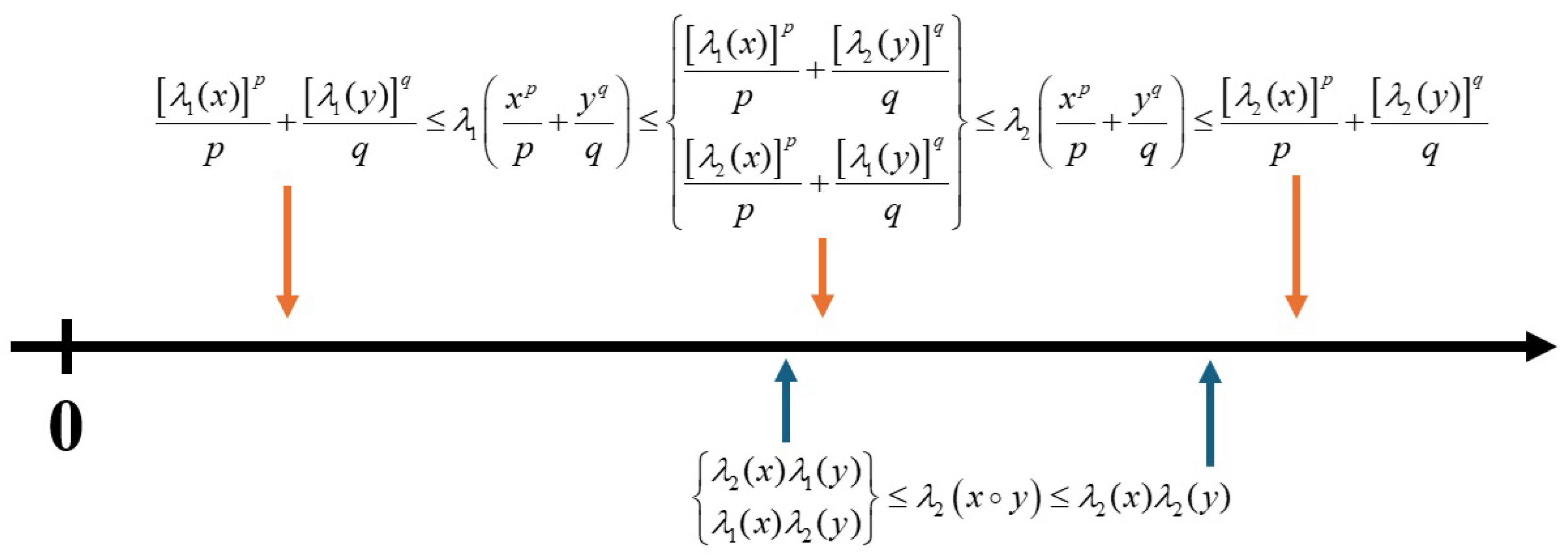
Proposition 1.

Suppose that $x,y\in {\mathcal{K}}^n$ and $1<p,q<\infty$ with ${\displaystyle \frac{1}{p}}+{\displaystyle \frac{1}{q}}=1$. Then, the following inequalities are satisfied:

(a) 

$min\left\{{\displaystyle \frac{{\left({\lambda }_1\left(x\right)\right)}^p}{p}}+{\displaystyle \frac{{\left({\lambda }_2\left(y\right)\right)}^q}{q}},{\displaystyle \frac{{\left({\lambda }_2\left(x\right)\right)}^p}{p}}+{\displaystyle \frac{{\left({\lambda }_1\left(y\right)\right)}^q}{q}}\right\}\ge {\lambda }_1\left({\displaystyle \frac{x^p}{p}}+{\displaystyle \frac{y^q}{q}}\right)\ge {\displaystyle \frac{{\left({\lambda }_1\left(x\right)\right)}^p}{p}}+{\displaystyle \frac{{\left({\lambda }_1\left(y\right)\right)}^q}{q}}$.

(b) 

$max\left\{{\displaystyle \frac{{\left({\lambda }_1\left(x\right)\right)}^p}{p}}+{\displaystyle \frac{{\left({\lambda }_2\left(y\right)\right)}^q}{q}},{\displaystyle \frac{{\left({\lambda }_2\left(x\right)\right)}^p}{p}}+{\displaystyle \frac{{\left({\lambda }_1\left(y\right)\right)}^q}{q}}\right\}\le {\lambda }_2\left({\displaystyle \frac{x^p}{p}}+{\displaystyle \frac{y^q}{q}}\right)\le {\displaystyle \frac{{\left({\lambda }_2\left(x\right)\right)}^p}{p}}+{\displaystyle \frac{{\left({\lambda }_2\left(y\right)\right)}^q}{q}}.$

Proof. 

According to the decomposition of $x,y$, it is clear that

$$\begin{array}{cc}\hfill {\lambda }_1\left({\displaystyle \frac{x^p}{p}}\right)& ={\displaystyle \frac{{\left({\lambda }_1\left(x\right)\right)}^p}{p}},{\lambda }_2\left({\displaystyle \frac{x^p}{p}}\right)={\displaystyle \frac{{\left({\lambda }_2\left(x\right)\right)}^p}{p}},\hfill \\ \hfill {\lambda }_1\left({\displaystyle \frac{y^q}{q}}\right)& ={\displaystyle \frac{{\left({\lambda }_1\left(y\right)\right)}^q}{q}},{\lambda }_2\left({\displaystyle \frac{y^q}{q}}\right)={\displaystyle \frac{{\left({\lambda }_2\left(y\right)\right)}^q}{q}},\hfill \end{array}$$

since p and q are positive and ${\lambda }_j\left(x\right),{\lambda }_j\left(y\right)\ge 0$ for $j=1,2$.

(a) It follows by Lemma 3 that

$$\begin{array}{cc}\hfill {\lambda }_1\left({\displaystyle \frac{x^p}{p}}+{\displaystyle \frac{y^q}{q}}\right)& \ge {\lambda }_1\left({\displaystyle \frac{x^p}{p}}\right)+{\lambda }_1\left({\displaystyle \frac{y^q}{q}}\right)={\displaystyle \frac{{\left({\lambda }_1\left(x\right)\right)}^p}{p}}+{\displaystyle \frac{{\left({\lambda }_1\left(y\right)\right)}^q}{q}},\hfill \\ \hfill {\lambda }_1\left({\displaystyle \frac{x^p}{p}}+{\displaystyle \frac{y^q}{q}}\right)& \le min\left\{{\lambda }_1\left({\displaystyle \frac{x^p}{p}}\right)+{\lambda }_2\left({\displaystyle \frac{y^q}{q}}\right),{\lambda }_2\left({\displaystyle \frac{x^p}{p}}\right)+{\lambda }_1\left({\displaystyle \frac{y^q}{q}}\right)\right\}\hfill \\ \hfill & =min\left\{{\displaystyle \frac{{\left({\lambda }_1\left(x\right)\right)}^p}{p}}+{\displaystyle \frac{{\left({\lambda }_2\left(y\right)\right)}^q}{q}},{\displaystyle \frac{{\left({\lambda }_2\left(x\right)\right)}^p}{p}}+{\displaystyle \frac{{\left({\lambda }_1\left(y\right)\right)}^q}{q}}\right\}.\hfill \end{array}$$

(b) Similarly, the desired inequality follows by

$$\begin{array}{cc}\hfill {\lambda }_2\left({\displaystyle \frac{x^p}{p}}+{\displaystyle \frac{y^q}{q}}\right)& \le {\lambda }_2\left({\displaystyle \frac{x^p}{p}}\right)+{\lambda }_2\left({\displaystyle \frac{y^q}{q}}\right)={\displaystyle \frac{{\left({\lambda }_2\left(x\right)\right)}^p}{p}}+{\displaystyle \frac{{\left({\lambda }_2\left(y\right)\right)}^q}{q}},\hfill \\ \hfill {\lambda }_2\left({\displaystyle \frac{x^p}{p}}+{\displaystyle \frac{y^q}{q}}\right)& \ge max\left\{{\lambda }_1\left({\displaystyle \frac{x^p}{p}}\right)+{\lambda }_2\left({\displaystyle \frac{y^q}{q}}\right),{\lambda }_2\left({\displaystyle \frac{x^p}{p}}\right)+{\lambda }_1\left({\displaystyle \frac{y^q}{q}}\right)\right\}\hfill \\ \hfill & =max\left\{{\displaystyle \frac{{\left({\lambda }_1\left(x\right)\right)}^p}{p}}+{\displaystyle \frac{{\left({\lambda }_2\left(y\right)\right)}^q}{q}},{\displaystyle \frac{{\left({\lambda }_2\left(x\right)\right)}^p}{p}}+{\displaystyle \frac{{\left({\lambda }_1\left(y\right)\right)}^q}{q}}\right\}.\hfill \end{array}$$

This completes the proof. □

Proposition 2.

Suppose that $x,y\in {\mathcal{K}}^n$. Then, the following inequality holds:

$$max\left\{{\lambda }_1\left(x\right){\lambda }_2\left(y\right),{\lambda }_2\left(x\right){\lambda }_1\left(y\right)\right\}\le {\lambda }_2(x\circ y)\le {\lambda }_2\left(x\right){\lambda }_2\left(y\right).$$

Proof. 

We note that $x\circ y=\left(x_1{y}_1+\langle x_2,y_2\rangle ,x_1{y}_2+y_1{x}_2\right)$, and hence,

$${\lambda }_2(x\circ y)=x_1{y}_1+\langle x_2,y_2\rangle +\parallel x_1{y}_2+y_1{x}_2\parallel .$$

Consequently, the result follows from

$$\begin{array}{cc}\hfill & max\left\{{\lambda }_1\left(x\right){\lambda }_2\left(y\right),{\lambda }_2\left(x\right){\lambda }_1\left(y\right)\right\}\hfill \\ \hfill & ={\displaystyle \frac{1}{2}}\left({\lambda }_1\left(x\right){\lambda }_2\left(y\right)+{\lambda }_2\left(x\right){\lambda }_1\left(y\right)+|{\lambda }_1\left(x\right){\lambda }_2\left(y\right)-{\lambda }_2\left(x\right){\lambda }_1\left(y\right)|\right)\hfill \\ \hfill & ={\displaystyle \frac{1}{2}}\left(2x_1{y}_1-2\parallel x_2\parallel \parallel y_2\parallel +|2x_1\parallel y_2\parallel -2y_1\parallel x_2\parallel |\right)\hfill \\ \hfill & =x_1{y}_1-\parallel x_2\parallel \parallel y_2\parallel +|x_1\parallel y_2\parallel -y_1\parallel x_2\parallel |\hfill \\ \hfill & \le x_1{y}_1+\langle x_2,y_2\rangle +\parallel x_1{y}_2+y_1{x}_2\parallel \hfill \\ \hfill & \le x_1{y}_1+\parallel x_2\parallel \parallel y_2\parallel +x_1\parallel y_2\parallel +y_1\parallel x_2\parallel \hfill \\ \hfill & ={\lambda }_2\left(x\right){\lambda }_2\left(y\right),\hfill \end{array}$$

where the inequalities hold by the triangle inequality for norms and the Cauchy–Schwarz inequality. □

Remark 1.

Based on Propositions 1–2, for $1<p,q<\infty$ with ${\displaystyle \frac{1}{p}}+{\displaystyle \frac{1}{q}}=1$, we can establish a picture of the ordered relationship between the eigenvalues of x, y, $x\circ y$, ${\displaystyle \frac{x^p}{p}}+{\displaystyle \frac{y^q}{q}}$ as depicted in Figure 1. However, we have no results regarding the relationship between ${\lambda }_1(x\circ y)$ and ${\lambda }_1\left(x\right){\lambda }_1\left(y\right)$. In fact, $x\circ y$ does not always belong to ${\mathcal{K}}^n$ even if $x,y\in {\mathcal{K}}^n$. That is, it is possible that ${\lambda }_1(x\circ y)\le {\lambda }_1\left(x\right){\lambda }_1\left(y\right)$.

Proposition 3.

Suppose that $x,y\in {\mathcal{K}}^n$, $1<p,q<\infty$ with ${\displaystyle \frac{1}{p}}+{\displaystyle \frac{1}{q}}=1$. Then, the following inequality holds:

$$\begin{array}{cc}\hfill & \left({\displaystyle \frac{{\left({\lambda }_1\left(x\right)\right)}^p}{p}}+{\displaystyle \frac{{\left({\lambda }_1\left(y\right)\right)}^q}{q}}\right)\left({\displaystyle \frac{{\left({\lambda }_2\left(x\right)\right)}^p}{p}}+{\displaystyle \frac{{\left({\lambda }_2\left(y\right)\right)}^q}{q}}\right)\hfill \\ \hfill & \le det\left({\displaystyle \frac{x^p}{p}}+{\displaystyle \frac{y^q}{q}}\right)\hfill \\ \hfill & \le \left({\displaystyle \frac{{\left({\lambda }_1\left(x\right)\right)}^p}{p}}+{\displaystyle \frac{{\left({\lambda }_2\left(y\right)\right)}^q}{q}}\right)\left({\displaystyle \frac{{\left({\lambda }_2\left(x\right)\right)}^p}{p}}+{\displaystyle \frac{{\left({\lambda }_1\left(y\right)\right)}^q}{q}}\right).\hfill \end{array}$$

Proof. 

First, we observe by a straightforward calculation that

$$\begin{array}{cc}\hfill {\displaystyle \frac{x^p}{p}}+{\displaystyle \frac{y^q}{q}}& =\left({\displaystyle \frac{{\left({\lambda }_1\left(x\right)\right)}^p}{p}}{u}_x^{\left(1\right)}+{\displaystyle \frac{{\left({\lambda }_2\left(x\right)\right)}^p}{p}}{u}_x^{\left(2\right)}\right)+\left({\displaystyle \frac{{\left({\lambda }_1\left(y\right)\right)}^q}{q}}{u}_y^{\left(1\right)}+{\displaystyle \frac{{\left({\lambda }_2\left(y\right)\right)}^q}{q}}{u}_y^{\left(2\right)}\right)\hfill \\ \hfill & =\left({\displaystyle \frac{{\left({\lambda }_1\left(x\right)\right)}^p+{\left({\lambda }_2\left(x\right)\right)}^p}{2p}},{\displaystyle \frac{{\left({\lambda }_2\left(x\right)\right)}^p-{\left({\lambda }_1\left(x\right)\right)}^p}{2p}}{\displaystyle \frac{x_2}{\parallel x_2\parallel }}\right)\hfill \\ \hfill & +\left({\displaystyle \frac{{\left({\lambda }_1\left(y\right)\right)}^q+{\left({\lambda }_2\left(y\right)\right)}^q}{2q}},{\displaystyle \frac{{\left({\lambda }_2\left(y\right)\right)}^q-{\left({\lambda }_1\left(y\right)\right)}^q}{2q}}{\displaystyle \frac{y_2}{\parallel y_2\parallel }}\right)\hfill \\ \hfill & :=(w_1,w_2),\hfill \end{array}$$

where

$$\begin{array}{cc}\hfill w_1& ={\displaystyle \frac{{\left({\lambda }_1\left(x\right)\right)}^p+{\left({\lambda }_2\left(x\right)\right)}^p}{2p}}+{\displaystyle \frac{{\left({\lambda }_1\left(y\right)\right)}^q+{\left({\lambda }_2\left(y\right)\right)}^q}{2q}},\hfill \\ \hfill w_2& ={\displaystyle \frac{{\left({\lambda }_2\left(x\right)\right)}^p-{\left({\lambda }_1\left(x\right)\right)}^p}{2p}}{\displaystyle \frac{x_2}{\parallel x_2\parallel }}+{\displaystyle \frac{{\left({\lambda }_2\left(y\right)\right)}^q-{\left({\lambda }_1\left(y\right)\right)}^q}{2q}}{\displaystyle \frac{y_2}{\parallel y_2\parallel }}.\hfill \end{array}$$

(6)

It follows from the triangle inequality for norms that

$$\begin{array}{cc}\hfill \parallel w_2{\parallel }^2& ={∥{\displaystyle \frac{{\left({\lambda }_2\left(x\right)\right)}^p-{\left({\lambda }_1\left(x\right)\right)}^p}{2p}}{\displaystyle \frac{x_2}{\parallel x_2\parallel }}+{\displaystyle \frac{{\left({\lambda }_2\left(y\right)\right)}^q-{\left({\lambda }_1\left(y\right)\right)}^q}{2q}}{\displaystyle \frac{y_2}{\parallel y_2\parallel }}∥}^2\hfill \\ \hfill & \le {\left(∥{\displaystyle \frac{{\left({\lambda }_2\left(x\right)\right)}^p-{\left({\lambda }_1\left(x\right)\right)}^p}{2p}}{\displaystyle \frac{x_2}{\parallel x_2\parallel }}∥+∥{\displaystyle \frac{{\left({\lambda }_2\left(y\right)\right)}^q-{\left({\lambda }_1\left(y\right)\right)}^q}{2q}}{\displaystyle \frac{y_2}{\parallel y_2\parallel }}∥\right)}^2\hfill \\ \hfill & ={\left({\displaystyle \frac{{\left({\lambda }_2\left(x\right)\right)}^p-{\left({\lambda }_1\left(x\right)\right)}^p}{2p}}+{\displaystyle \frac{{\left({\lambda }_2\left(y\right)\right)}^q-{\left({\lambda }_1\left(y\right)\right)}^q}{2q}}\right)}^2,\hfill \end{array}$$

and similarly,

$$\begin{array}{cc}\hfill \parallel w_2{\parallel }^2& \ge {\left|∥{\displaystyle \frac{{\left({\lambda }_2\left(x\right)\right)}^p-{\left({\lambda }_1\left(x\right)\right)}^p}{2p}}{\displaystyle \frac{x_2}{\parallel x_2\parallel }}∥-∥{\displaystyle \frac{{\left({\lambda }_2\left(y\right)\right)}^q-{\left({\lambda }_1\left(y\right)\right)}^q}{2q}}{\displaystyle \frac{y_2}{\parallel y_2\parallel }}∥\right|}^2\hfill \\ \hfill & ={\left({\displaystyle \frac{{\left({\lambda }_2\left(x\right)\right)}^p-{\left({\lambda }_1\left(x\right)\right)}^p}{2p}}-{\displaystyle \frac{{\left({\lambda }_2\left(y\right)\right)}^q-{\left({\lambda }_1\left(y\right)\right)}^q}{2q}}\right)}^2,\hfill \end{array}$$

since $0\le {\lambda }_1\left(x\right)\le {\lambda }_2\left(x\right)$ and $0\le {\lambda }_1\left(y\right)\le {\lambda }_2\left(y\right)$. In combining the above inequalities with the definition of a determinant, the first part of the desired inequality follows from

$$\begin{array}{cc}\hfill det\left({\displaystyle \frac{x^p}{p}}+{\displaystyle \frac{y^q}{q}}\right)& =w_1^2-{\parallel w_2\parallel }^2\hfill \\ \hfill & \ge {\left({\displaystyle \frac{{\left({\lambda }_1\left(x\right)\right)}^p+{\left({\lambda }_2\left(x\right)\right)}^p}{2p}}+{\displaystyle \frac{{\left({\lambda }_1\left(y\right)\right)}^q+{\left({\lambda }_2\left(y\right)\right)}^q}{2q}}\right)}^2\hfill \\ \hfill & -{\left({\displaystyle \frac{{\left[{\lambda }_2\left(x\right)\right]}^p-{\left[{\lambda }_1\left(x\right)\right]}^p}{2p}}+{\displaystyle \frac{{\left({\lambda }_2\left(y\right)\right)}^q-{\left({\lambda }_1\left(y\right)\right)}^q}{2q}}\right)}^2\hfill \\ \hfill & ={\displaystyle \frac{{\left({\lambda }_1\left(x\right)\right)}^p{\left({\lambda }_2\left(x\right)\right)}^p}{p^2}}+{\displaystyle \frac{{\left({\lambda }_1\left(y\right)\right)}^q{\left({\lambda }_2\left(y\right)\right)}^q}{q^2}}\hfill \\ \hfill & +{\displaystyle \frac{{\left({\lambda }_1\left(x\right)\right)}^p{\left({\lambda }_2\left(y\right)\right)}^q+{\left({\lambda }_2\left(x\right)\right)}^p{\left({\lambda }_1\left(y\right)\right)}^q}{pq}}\hfill \\ \hfill & =\left({\displaystyle \frac{{\left({\lambda }_1\left(x\right)\right)}^p}{p}}+{\displaystyle \frac{{\left({\lambda }_1\left(y\right)\right)}^q}{q}}\right)\left({\displaystyle \frac{{\left({\lambda }_2\left(x\right)\right)}^p}{p}}+{\displaystyle \frac{{\left({\lambda }_2\left(y\right)\right)}^q}{q}}\right).\hfill \end{array}$$

Likewise, the second inequality is valid since

$$\begin{array}{cc}\hfill det\left({\displaystyle \frac{x^p}{p}}+{\displaystyle \frac{y^q}{q}}\right)& \le {\left({\displaystyle \frac{{\left({\lambda }_1\left(x\right)\right)}^p+{\left({\lambda }_2\left(x\right)\right)}^p}{2p}}+{\displaystyle \frac{{\left({\lambda }_1\left(y\right)\right)}^q+{\left({\lambda }_2\left(y\right)\right)}^q}{2q}}\right)}^2\hfill \\ \hfill & -{\left({\displaystyle \frac{{\left({\lambda }_2\left(x\right)\right)}^p-{\left({\lambda }_1\left(x\right)\right)}^p}{2p}}-{\displaystyle \frac{{\left({\lambda }_2\left(y\right)\right)}^q-{\left({\lambda }_1\left(y\right)\right)}^q}{2q}}\right)}^2\hfill \\ \hfill & ={\displaystyle \frac{{\left({\lambda }_1\left(x\right)\right)}^p{\left({\lambda }_2\left(x\right)\right)}^p}{p^2}}+{\displaystyle \frac{{\left({\lambda }_1\left(y\right)\right)}^q{\left({\lambda }_2\left(y\right)\right)}^q}{q^2}}\hfill \\ \hfill & +{\displaystyle \frac{{\left({\lambda }_1\left(x\right)\right)}^p{\left({\lambda }_1\left(y\right)\right)}^q+{\left({\lambda }_2\left(x\right)\right)}^p{\left({\lambda }_2\left(y\right)\right)}^q}{pq}}\hfill \\ \hfill & =\left({\displaystyle \frac{{\left({\lambda }_1\left(x\right)\right)}^p}{p}}+{\displaystyle \frac{{\left({\lambda }_2\left(y\right)\right)}^q}{q}}\right)\left({\displaystyle \frac{{\left({\lambda }_2\left(x\right)\right)}^p}{p}}+{\displaystyle \frac{{\left({\lambda }_1\left(y\right)\right)}^q}{q}}\right).\hfill \end{array}$$

Therefore, we conclude the desired inequalities. □

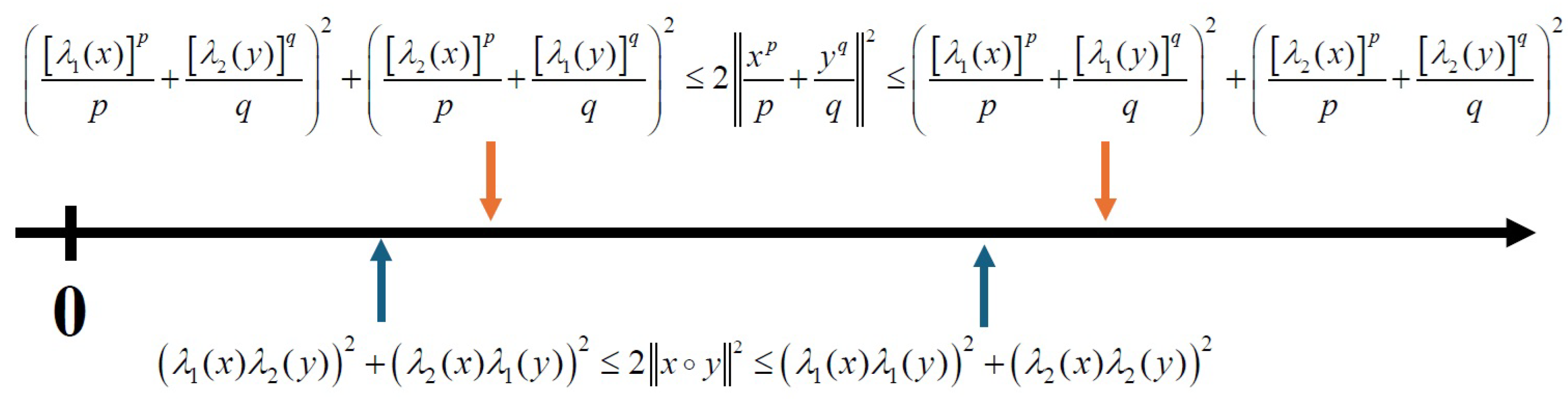
Remark 2.

According to Lemma 2 and the classical Young inequality for real numbers, we obtain a determinant version of Young’s inequality associated with second-order cones. Specifically, for $x,y\in {\mathcal{K}}^n$ and $1<p,q<\infty$ with ${\displaystyle \frac{1}{p}}+{\displaystyle \frac{1}{q}}=1$, we conclude that

$$\begin{array}{cc}\hfill det(x\circ y)& \le det\left(x\right)det\left(y\right)\hfill \\ \hfill & ={\lambda }_1\left(x\right){\lambda }_2\left(x\right){\lambda }_1\left(y\right){\lambda }_2\left(y\right)\hfill \\ \hfill & \le \left({\displaystyle \frac{{\left({\lambda }_1\left(x\right)\right)}^p}{p}}+{\displaystyle \frac{{\left({\lambda }_1\left(y\right)\right)}^q}{q}}\right)\left({\displaystyle \frac{{\left({\lambda }_2\left(x\right)\right)}^p}{p}}+{\displaystyle \frac{{\left({\lambda }_2\left(y\right)\right)}^q}{q}}\right)\hfill \\ \hfill & \le det\left({\displaystyle \frac{x^p}{p}}+{\displaystyle \frac{y^q}{q}}\right).\hfill \end{array}$$

In fact, Huang et al. [5] established the determinant version of Young’s inequality based on the SOC weighted mean inequality. However, we obtain a refined inequality by direct computation.

Proposition 4.

Suppose that $x,y\in {\mathcal{K}}^n$, $1<p,q<\infty$ with ${\displaystyle \frac{1}{p}}+{\displaystyle \frac{1}{q}}=1$. Then the following inequality holds.

$$\begin{array}{cc}\hfill & {\left({\displaystyle \frac{{\left({\lambda }_1\left(x\right)\right)}^p}{p}}+{\displaystyle \frac{{\left({\lambda }_2\left(y\right)\right)}^q}{q}}\right)}^2+{\left({\displaystyle \frac{{\left({\lambda }_2\left(x\right)\right)}^p}{p}}+{\displaystyle \frac{{\left({\lambda }_1\left(y\right)\right)}^q}{q}}\right)}^2\hfill \\ \hfill & \le 2{∥{\displaystyle \frac{x^p}{p}}+{\displaystyle \frac{y^q}{q}}∥}^2\hfill \\ \hfill & \le {\left({\displaystyle \frac{{\left({\lambda }_1\left(x\right)\right)}^p}{p}}+{\displaystyle \frac{{\left({\lambda }_1\left(y\right)\right)}^q}{q}}\right)}^2+{\left({\displaystyle \frac{{\left({\lambda }_2\left(x\right)\right)}^p}{p}}+{\displaystyle \frac{{\left({\lambda }_2\left(y\right)\right)}^q}{q}}\right)}^2.\hfill \end{array}$$

Proof. 

Let ${\displaystyle \frac{x^p}{p}+\frac{y^q}{q}}$ be expressed as in (6). Following the similar argument in Proposition 3, we deduce that

$$\begin{array}{cc}\hfill 2{∥{\displaystyle \frac{x^p}{p}}+{\displaystyle \frac{y^q}{q}}∥}^2& =2\left(w_1^2+{\parallel w_2\parallel }^2\right)\hfill \\ \hfill & \le 2{\left({\displaystyle \frac{{\left({\lambda }_1\left(x\right)\right)}^p+{\left({\lambda }_2\left(x\right)\right)}^p}{2p}}+{\displaystyle \frac{{\left({\lambda }_1\left(y\right)\right)}^q+{\left({\lambda }_2\left(y\right)\right)}^q}{2q}}\right)}^2\hfill \\ \hfill & +2{\left({\displaystyle \frac{{\left({\lambda }_2\left(x\right)\right)}^p-{\left({\lambda }_1\left(x\right)\right)}^p}{2p}}+{\displaystyle \frac{{\left({\lambda }_2\left(y\right)\right)}^q-{\left({\lambda }_1\left(y\right)\right)}^q}{2q}}\right)}^2\hfill \\ \hfill & ={\displaystyle \frac{{\left({\lambda }_1\left(x\right)\right)}^{2p}+{\left({\lambda }_2\left(x\right)\right)}^{2p}}{p^2}}+{\displaystyle \frac{{\left({\lambda }_1\left(y\right)\right)}^{2q}+{\left({\lambda }_2\left(y\right)\right)}^{2q}}{q^2}}\hfill \\ \hfill & +{\displaystyle \frac{2{\left({\lambda }_1\left(x\right)\right)}^p{\left({\lambda }_1\left(y\right)\right)}^q+2{\left({\lambda }_2\left(x\right)\right)}^p{\left({\lambda }_2\left(y\right)\right)}^q}{pq}}\hfill \\ \hfill & ={\left({\displaystyle \frac{{\left({\lambda }_1\left(x\right)\right)}^p}{p}}+{\displaystyle \frac{{\left({\lambda }_1\left(y\right)\right)}^q}{q}}\right)}^2+{\left({\displaystyle \frac{{\left({\lambda }_2\left(x\right)\right)}^p}{p}}+{\displaystyle \frac{{\left({\lambda }_2\left(y\right)\right)}^q}{q}}\right)}^2.\hfill \end{array}$$

Similarly, the other inequality holds by

$$\begin{array}{cc}\hfill 2{∥{\displaystyle \frac{x^p}{p}}+{\displaystyle \frac{y^q}{q}}∥}^2& \ge 2{\left({\displaystyle \frac{{\left({\lambda }_1\left(x\right)\right)}^p+{\left({\lambda }_2\left(x\right)\right)}^p}{2p}}+{\displaystyle \frac{{\left({\lambda }_1\left(y\right)\right)}^q+{\left({\lambda }_2\left(y\right)\right)}^q}{2q}}\right)}^2\hfill \\ \hfill & +2{\left({\displaystyle \frac{{\left({\lambda }_2\left(x\right)\right)}^p-{\left({\lambda }_1\left(x\right)\right)}^p}{2p}}-{\displaystyle \frac{{\left({\lambda }_2\left(y\right)\right)}^q-{\left({\lambda }_1\left(y\right)\right)}^q}{2q}}\right)}^2\hfill \\ \hfill & ={\displaystyle \frac{{\left({\lambda }_1\left(x\right)\right)}^{2p}+{\left({\lambda }_2\left(x\right)\right)}^{2p}}{p^2}}+{\displaystyle \frac{{\left({\lambda }_1\left(y\right)\right)}^{2q}+{\left({\lambda }_2\left(y\right)\right)}^{2q}}{q^2}}\hfill \\ \hfill & +{\displaystyle \frac{2{\left({\lambda }_1\left(x\right)\right)}^p{\left({\lambda }_2\left(y\right)\right)}^q+2{\left({\lambda }_2\left(x\right)\right)}^p{\left({\lambda }_1\left(y\right)\right)}^q}{pq}}\hfill \\ \hfill & ={\left({\displaystyle \frac{{\left({\lambda }_1\left(x\right)\right)}^p}{p}}+{\displaystyle \frac{{\left({\lambda }_2\left(y\right)\right)}^q}{q}}\right)}^2+{\left({\displaystyle \frac{{\left({\lambda }_2\left(x\right)\right)}^p}{p}}+{\displaystyle \frac{{\left({\lambda }_1\left(y\right)\right)}^q}{q}}\right)}^2.\hfill \end{array}$$

Thus, the desired result follows. □

Proposition 5.

Suppose that $x,y\in {\mathcal{K}}^n$. Then, the following inequality holds

$${\left({\lambda }_1\left(x\right){\lambda }_2\left(y\right)\right)}^2+{\left({\lambda }_2\left(x\right){\lambda }_1\left(y\right)\right)}^2\le 2{∥x\circ y∥}^2\le {\left({\lambda }_1\left(x\right){\lambda }_1\left(y\right)\right)}^2+{\left({\lambda }_2\left(x\right){\lambda }_2\left(y\right)\right)}^2.$$

Proof. 

It is evident that the inequalities hold if $x_2=\mathbf{0}$ or $y_2=\mathbf{0}$. In fact, the equality will hold if $x_2=\mathbf{0}$ or $y_2=\mathbf{0}$. Assume that $x_2\ne \mathbf{0}$ and $y_2\ne \mathbf{0}$, which implies $x_1>0$ and $y_1>0$. Then,

$$\begin{array}{cc}\hfill {∥x\circ y∥}^2& ={(x_1{y}_1+\langle x_2,y_2\rangle )}^2+{\parallel x_1{y}_2+y_1{x}_2\parallel }^2\hfill \\ \hfill & =x_1^2{y}_1^2+{\left(\langle x_2,y_2\rangle \right)}^2+x_1^2\parallel y_2{\parallel }^2+y_1^2{\parallel x_2\parallel }^2+4x_1{y}_1\langle x_2,y_2\rangle \hfill \\ \hfill & =x_1^2{y}_1^2+\parallel x_2{\parallel }^2\parallel y_2{\parallel }^2{cos}^2\theta +x_1^2\parallel y_2{\parallel }^2+y_1^2\parallel x_2{\parallel }^2+4x_1{y}_1\parallel x_2\parallel \parallel y_2\parallel cos\theta ,\hfill \end{array}$$

where $\theta$ is the angle between $x_2$ and $y_2$ in ${\mathbb{R}}^{n-1}$. We notice that the value of $2{∥x\circ y∥}^2$ is determined by $\theta$ if $x_1$, $y_1$, $\parallel x_2\parallel$, and $\parallel y_2\parallel$ are fixed. Let $f:[0,\pi ]\to \mathbb{R}$ be defined by

$$f\left(\theta \right)=\parallel x_2{\parallel }^2\parallel y_2{\parallel }^2{cos}^2\theta +4x_1{y}_1\parallel x_2\parallel \parallel y_2\parallel cos\theta .$$

The derivative of f is

$$\begin{array}{cc}\hfill f^{\prime }\left(\theta \right)& =-2\parallel x_2{\parallel }^2\parallel y_2{\parallel }^{2}cos\theta sin\theta -4x_1{y}_1\parallel x_2\parallel \parallel y_2\parallel sin\theta \hfill \\ \hfill & =-2\parallel x_2\parallel \parallel y_2\parallel sin\theta \left(\parallel x_2\parallel \parallel y_2\parallel cos\theta +2x_1{y}_1\right).\hfill \end{array}$$

Then, it is clear that 0 and $\pi$ are the only two critical points of f since

$$\begin{array}{cc}\hfill \parallel x_2\parallel \parallel y_2\parallel cos\theta +2x_1{y}_1& =x_1{y}_1+(x_1{y}_1+\parallel x_2\parallel \parallel y_2\parallel cos\theta )\hfill \\ \hfill & \ge x_1{y}_1+(\parallel x_2\parallel \parallel y_2\parallel +\parallel x_2\parallel \parallel y_2\parallel cos\theta )\hfill \\ \hfill & >0.\hfill \end{array}$$

Therefore, the extreme values of $2{∥x\circ y∥}^2$ occur at $\theta =0,\pi$. For $\theta =0$, we have

$$\begin{array}{cc}\hfill 2{∥x\circ y∥}^2& =2\left(x_1^2{y}_1^2+\parallel x_2{\parallel }^2\parallel y_2{\parallel }^2+x_1^2\parallel y_2{\parallel }^2+y_1^2\parallel x_2{\parallel }^2+4x_1{y}_1\parallel x_2\parallel \parallel y_2\parallel \right)\hfill \\ \hfill & ={\left({\lambda }_1\left(x\right){\lambda }_1\left(y\right)\right)}^2+{\left({\lambda }_2\left(x\right){\lambda }_2\left(y\right)\right)}^2.\hfill \end{array}$$

On the other hand, for $\theta =\pi$, we obtain

$$\begin{array}{cc}\hfill 2{∥x\circ y∥}^2& =2\left(x_1^2{y}_1^2+\parallel x_2{\parallel }^2\parallel y_2{\parallel }^2+x_1^2\parallel y_2{\parallel }^2+y_1^2\parallel x_2{\parallel }^2-4x_1{y}_1\parallel x_2\parallel \parallel y_2\parallel \right)\hfill \\ \hfill & ={\left({\lambda }_1\left(x\right){\lambda }_2\left(y\right)\right)}^2+{\left({\lambda }_2\left(x\right){\lambda }_1\left(y\right)\right)}^2.\hfill \end{array}$$

Thus, the norm $2{∥x\circ y∥}^2$ achieves its maximum and minimum at $\theta =0$ and $\theta =\pi$, respectively. The proof is complete. □

Remark 3.

According to the proof of Proposition 4, we remark that the maximum and minimum of the norm $2{∥{\displaystyle \frac{x^p}{p}}+{\displaystyle \frac{y^q}{q}}∥}^2$ also occur at $\theta =0$ and $\theta =\pi$, respectively. In addition, for $1<p,q<\infty$ with ${\displaystyle \frac{1}{p}}+{\displaystyle \frac{1}{q}}=1$, we could obtain the relationship between these two maxima and minima by applying the classical Young inequality; see Figure 2. However, we have not reached a conclusion on whether the inequality $∥x\circ y∥\le ∥{\displaystyle \frac{x^p}{p}}+{\displaystyle \frac{y^q}{q}}∥$ is true or not.

In the following, we investigate the inverse Young inequality associated with second-order cones and its applications. We first review the classic inverse Young inequality in $\mathbb{R}$, namely

$$ab\ge \nu b^{{\displaystyle \frac{1}{\nu }}}+(1-\nu )a^{{\displaystyle \frac{1}{1-\nu }}},$$

for $a,b>0$ and $\nu >1$. In the context of matrix analysis, Manjegani and Norouzi [21] established an inverse Young inequality for eigenvalues. Specifically, for all $1\le j\le n$ and $\nu >1$,

$$s_j\left(AB\right)\ge s_j\left(\nu A^{{\displaystyle \frac{1}{\nu }}}+(1-\nu )B^{{\displaystyle \frac{1}{1-\nu }}}\right),$$

(7)

where A and B are positive definite matrices. However, Drury [22] provided counterexamples to inequality (7) for $\nu =2$, and then modified it slightly. He proved that inequality (7) holds only for $1<\nu <{\displaystyle \frac{3}{2}}$. In the following, we first discuss the trace version of the inverse Young inequality associated with second-order cones.

Theorem 2.

(Inverse Young inequality—Type I) Suppose that $x,y\in \mathrm{int}\left({\mathcal{K}}^n\right)$ and $\nu >1$. Then, the following inequality holds:

$$\mathrm{tr}(x\circ y)\ge \mathrm{tr}\left(\nu x^{{\displaystyle \frac{1}{\nu }}}+(1-\nu )y^{{\displaystyle \frac{1}{1-\nu }}}\right).$$

Proof. 

According to Lemma 1(e) and (f), the desired result follows from the following computation:

$$\begin{array}{cc}\hfill \mathrm{tr}(x\circ y)& \ge {\lambda }_1\left(x\right){\lambda }_2\left(y\right)+{\lambda }_2\left(x\right){\lambda }_1\left(y\right)\hfill \\ \hfill & \ge \left(\nu {\left({\lambda }_1\left(x\right)\right)}^{{\displaystyle \frac{1}{\nu }}}+(1-\nu ){\left({\lambda }_2\left(y\right)\right)}^{{\displaystyle \frac{1}{1-\nu }}}\right)+\left(\nu {\left({\lambda }_2\left(x\right)\right)}^{{\displaystyle \frac{1}{\nu }}}+(1-\nu ){\left({\lambda }_1\left(y\right)\right)}^{{\displaystyle \frac{1}{1-\nu }}}\right)\hfill \\ \hfill & =\nu \left({\left({\lambda }_1\left(x\right)\right)}^{{\displaystyle \frac{1}{\nu }}}+{\left({\lambda }_2\left(x\right)\right)}^{{\displaystyle \frac{1}{\nu }}}\right)+(1-\nu )\left({\left({\lambda }_1\left(y\right)\right)}^{{\displaystyle \frac{1}{1-\nu }}}+{\left({\lambda }_2\left(y\right)\right)}^{{\displaystyle \frac{1}{1-\nu }}}\right)\hfill \\ \hfill & =\mathrm{tr}(\nu x^{{\displaystyle \frac{1}{\nu }}}+(1-\nu )y^{{\displaystyle \frac{1}{1-\nu }}}),\hfill \end{array}$$

where the second inequality follows from the inverse Young inequality in ${\mathbb{R}}^n$. □

Corollary 1.

(Inverse Young inequality—Type II) Suppose that $x,y\in \mathrm{int}\left({\mathcal{K}}^n\right)$ and $\nu >1$. Then, the following inequality holds:

$$\mathrm{tr}\left(\right|x\circ y\left|\right)\ge \mathrm{tr}\left(\nu x^{{\displaystyle \frac{1}{\nu }}}+(1-\nu )y^{{\displaystyle \frac{1}{1-\nu }}}\right).$$

Proof. 

Since $|x\circ y|{⪰}_{{\mathcal{K}}^n}x\circ y$, the results follow immediately from Lemma 1(d) and Theorem 2. □

Corollary 2.

(Inverse Young inequality—Type III) Suppose that $x,y\in {\mathbb{R}}^n$ and $\nu >1$. If x and y are not in $\partial \left({\mathcal{K}}^n\right)\cup (-\partial \left({\mathcal{K}}^n\right))$, then the following inequality is satisfied:

$$\mathrm{tr}\left(\right|x|\circ \left|y\right|)\ge \mathrm{tr}\left({\nu \left|x\right|}^{{\displaystyle \frac{1}{\nu }}}+(1-\nu ){\left|y\right|}^{{\displaystyle \frac{1}{1-\nu }}}\right).$$

Proof. 

Since x and y are not in $\partial \left({\mathcal{K}}^n\right)\cup (-\partial \left({\mathcal{K}}^n\right))$, it follows from Lemma 1(a)–(c) that $\left|x\right|$ and $\left|y\right|$ are both in $\mathrm{int}\left({\mathcal{K}}^n\right)$. Therefore, the desired inequality is obtained by applying Theorem 2 to $\left|x\right|$ and $\left|y\right|$. □

Analogously to the classical setting in real analysis, we derive the trace versions of the inverse Hölder inequality by applying the trace versions of the inverse Young inequality through a similar analytical approach.

Theorem 3.

(Inverse Hölder inequality—Type I) Suppose that $x,y\in \mathrm{int}\left({\mathcal{K}}^n\right)$ and $\nu >1$. Then, the following inequality is satisfied:

$$\mathrm{tr}(x\circ y)\ge {\left[\mathrm{tr}\left(x^{{\displaystyle \frac{1}{\nu }}}\right)\right]}^{\nu }·{\left[\mathrm{tr}\left(y^{{\displaystyle \frac{1}{1-\nu }}}\right)\right]}^{1-\nu }.$$

Proof. 

Let $a={\left[\mathrm{tr}\left(x^{{\displaystyle \frac{1}{\nu }}}\right)\right]}^{\nu }$, $b={\left[\mathrm{tr}\left(y^{{\displaystyle \frac{1}{1-\nu }}}\right)\right]}^{1-\nu }$. Since $x,y\in \mathrm{int}\left({\mathcal{K}}^n\right)$, this implies that $a>0$ and $b>0$. Applying Theorem 2 to ${\displaystyle \frac{x}{a}}$ and ${\displaystyle \frac{y}{b}}$, we obtain

$$\begin{array}{cc}\hfill \mathrm{tr}\left({\displaystyle \frac{x}{a}}\circ {\displaystyle \frac{y}{b}}\right)& \ge \mathrm{tr}\left(\nu {\left({\displaystyle \frac{x}{a}}\right)}^{{\displaystyle \frac{1}{\nu }}}+(1-\nu ){\left({\displaystyle \frac{y}{b}}\right)}^{{\displaystyle \frac{1}{1-\nu }}}\right)\hfill \\ \hfill & =\nu \mathrm{tr}\left({\displaystyle \frac{x^{\frac{1}{\nu }}}{a^{\frac{1}{\nu }}}}\right)+(1-\nu )\mathrm{tr}\left({\displaystyle \frac{y^{\frac{1}{1-\nu }}}{b^{\frac{1}{1-\nu }}}}\right)\hfill \\ \hfill & =\nu {\displaystyle \frac{\mathrm{tr}\left(x^{\frac{1}{\nu }}\right)}{a^{\frac{1}{\nu }}}}+(1-\nu ){\displaystyle \frac{\mathrm{tr}\left(y^{\frac{1}{1-\nu }}\right)}{b^{\frac{1}{1-\nu }}}}\hfill \\ \hfill & =\nu +(1-\nu )\hfill \\ \hfill & =1.\hfill \end{array}$$

Multiplying both sides by $a·b$, we obtain

$$\mathrm{tr}(x\circ y)\ge a·b={\left[\mathrm{tr}(x^{{\displaystyle \frac{1}{\nu }}})\right]}^{\nu }·{\left[\mathrm{tr}(y^{{\displaystyle \frac{1}{1-\nu }}})\right]}^{1-\nu },$$

since $a,b>0$. □

Corollary 3.

(Inverse Hölder inequality—Type II) Suppose that $x,y\in {\mathbb{R}}^n$ and $\nu >1$. If x and y are not in $\partial \left({\mathcal{K}}^n\right)\cup (-\partial \left({\mathcal{K}}^n\right))$, then the following inequality is satisfied:

$$\mathrm{tr}\left(\right|x|\circ \left|y\right|)\ge {\left[\mathrm{tr}\left(\right|x{|}^{{\displaystyle \frac{1}{\nu }}})\right]}^{\nu }·{\left[\mathrm{tr}\left(\right|y{|}^{{\displaystyle \frac{1}{1-\nu }}})\right]}^{1-\nu }.$$

Proof. 

Following the similar argument in Corollary 2, the desired inequality follows by applying Theorem 3 to $\left|x\right|$ and $\left|y\right|$. □

Next, we apply the trace version of the inverse Hölder inequality to establish the trace version of the inverse Minkowski inequality.

Theorem 4.

(Inverse Minkowski inequality) Suppose that $x,y\in \mathrm{int}\left({\mathcal{K}}^n\right)$ and $\nu >1$. Then, the following inequality is satisfied:

$${\left[\mathrm{tr}\left({(x+y)}^{{\displaystyle \frac{1}{\nu }}}\right)\right]}^{\nu }\ge {\left[\mathrm{tr}\left(x^{{\displaystyle \frac{1}{\nu }}}\right)\right]}^{\nu }+{\left[\mathrm{tr}\left(y^{{\displaystyle \frac{1}{\nu }}}\right)\right]}^{\nu }.$$

Proof. 

By Lemma 1(e) and the distributive property of the Jordan product, we can write

$$\begin{array}{cc}\hfill \mathrm{tr}\left({(x+y)}^{{\displaystyle \frac{1}{\nu }}}\right)& =\mathrm{tr}\left((x+y)\circ {(x+y)}^{{\displaystyle \frac{1}{\nu }}-1}\right)\hfill \\ \hfill & =\mathrm{tr}\left(x\circ {(x+y)}^{{\displaystyle \frac{1}{\nu }}-1}\right)+\mathrm{tr}\left(y\circ {(x+y)}^{{\displaystyle \frac{1}{\nu }}-1}\right).\hfill \end{array}$$

Since $x+y$ is also in $\mathrm{int}\left({\mathcal{K}}^n\right)$, we apply Theorem 3 to each term in the above expression, and thus obtain

$$\begin{array}{cc}\hfill & \mathrm{tr}\left(x\circ {(x+y)}^{{\displaystyle \frac{1}{\nu }}-1}\right)+\mathrm{tr}\left(y\circ {(x+y)}^{{\displaystyle \frac{1}{\nu }}-1}\right)\hfill \\ \hfill & \ge {\left[\mathrm{tr}\left(x^{{\displaystyle \frac{1}{\nu }}}\right)\right]}^{\nu }·{\left[\mathrm{tr}\left({(x+y)}^{{\displaystyle \frac{1-\nu }{\nu }}·{\displaystyle \frac{1}{1-\nu }}}\right)\right]}^{1-\nu }+{\left[\mathrm{tr}\left(y^{{\displaystyle \frac{1}{\nu }}}\right)\right]}^{\nu }·{\left[\mathrm{tr}\left({(x+y)}^{{\displaystyle \frac{1-\nu }{\nu }}·{\displaystyle \frac{1}{1-\nu }}}\right)\right]}^{1-\nu }\hfill \\ \hfill & =\left({\left[\mathrm{tr}\left(x^{{\displaystyle \frac{1}{\nu }}}\right)\right]}^{\nu }+{\left[\mathrm{tr}\left(y^{{\displaystyle \frac{1}{\nu }}}\right)\right]}^{\nu }\right)·{\left[\mathrm{tr}\left({(x+y)}^{{\displaystyle \frac{1}{\nu }}}\right)\right]}^{1-\nu },\hfill \end{array}$$

Dividing both sides by ${\left[\mathrm{tr}\left({(x+y)}^{{\displaystyle \frac{1}{\nu }}}\right)\right]}^{1-\nu }$, which is positive since $x+y\in \mathrm{int}\left({\mathcal{K}}^n\right)$, we obtain ${\left[\mathrm{tr}\left({(x+y)}^{{\displaystyle \frac{1}{\nu }}}\right)\right]}^{\nu }\ge \left({\left[\mathrm{tr}\left(x^{{\displaystyle \frac{1}{\nu }}}\right)\right]}^{\nu }+{\left[\mathrm{tr}\left(y^{{\displaystyle \frac{1}{\nu }}}\right)\right]}^{\nu }\right)$ as required. □

Remark 4.

We provide a more detailed discussion of Theorem 4. Let $p={\displaystyle \frac{1}{\nu }}$. Then, the trace version of the inverse Minkowski inequality can be equivalently rewritten as

$${\left[\mathrm{tr}\left({(x+y)}^p\right)\right]}^{{\displaystyle \frac{1}{p}}}\ge {\left[\mathrm{tr}\left(x^p\right)\right]}^{{\displaystyle \frac{1}{p}}}+{\left[\mathrm{tr}\left(y^p\right)\right]}^{{\displaystyle \frac{1}{p}}},$$

where $0<p<1$. Huang et al. [6] showed that the quantity

$${\left|\right|\left|x\right|\left|\right|}_p:={\left[\mathrm{tr}\right(\left|x\right|}^p{\left)\right]}^{{\displaystyle \frac{1}{p}}},$$

defines a quasinorm on ${\mathbb{R}}^n$, known as the Schatten p-quasinorm. More recently, Jeong [23] established that this expression also defines a quasinorm on Euclidean Jordan algebras. In fact, it is analogous to the Schatten p-norm (or quasi-norm), which is defined via the p-norm of the singular values of a matrix; see [3] for further discussion. Combining ([6], Theorem 3.7) with Theorem 4, we can conclude that for all $x,y\in \mathrm{int}\left({\mathcal{K}}^n\right)$,

$${\left|\right|\left|x\right|\left|\right|}_p+{\left|\right|\left|y\right|\left|\right|}_p\le \left|\right||x+{y\left|\right||}_p\le 2^{{\displaystyle \frac{1}{p}}-1}\left({\left|\right|\left|x\right|\left|\right|}_p+{\left|\right|\left|y\right|\left|\right|}_p\right),$$

where $0<p<1$.

At the end of this section, we provide counterexamples to illustrate that the eigenvalue version of the inverse Young inequality associated with second-order cones does not always hold. That is, for all $x,y\in \mathrm{int}\left({\mathcal{K}}^n\right)$, the inequality

$${\lambda }_j(x\circ y)\ge {\lambda }_j\left(\nu x^{{\displaystyle \frac{1}{\nu }}}+(1-\nu )y^{{\displaystyle \frac{1}{1-\nu }}}\right),$$

fails to hold for all $j=1,2$ when $v=2$.

Example 1.

Let $x=(5,0,-2)$, $y=(5,-4,2)$. Then, we compute

$$\begin{array}{cc}\hfill x\circ y& =(21,-20,0),\hfill \\ \hfill x^{{\displaystyle \frac{1}{2}}}& =(2.1889,0,-0.4569),\hfill \\ \hfill y^{-1}& =(1,0.8,-0.4),\hfill \end{array}$$

and thus, $2x^{{\displaystyle \frac{1}{2}}}-y^{-1}\approx (3.3778,-0.8,-0.5137)$. Consequently, we obtain

$${\lambda }_1(x\circ y)=1<2.42707\approx {\lambda }_1(2x^{{\displaystyle \frac{1}{2}}}-y^{-1}).$$

Example 2.

Let $x=(5.5,0,-4)$, $y=(5.5,-3,4)$. Then, we compute

$$\begin{array}{cc}\hfill x\circ y& =(14.25,-16.5,0),\hfill \\ \hfill x^{{\displaystyle \frac{1}{2}}}& \approx (2.1535,0,-0.9287),\hfill \\ \hfill y^{-1}& \approx (1.0476,0.5714,-0.7619),\hfill \end{array}$$

which yields $2x^{{\displaystyle \frac{1}{2}}}-y^{-1}\approx (3.2593,-0.5714,-1.0956)$. Hence, the eigenvalues of $x\circ y$ and $2x^{{\displaystyle \frac{1}{2}}}-y^{-1}$ are derived by

$$\begin{array}{cc}\hfill {\lambda }_1(x\circ y)=-2.25& ,{\lambda }_1(2x^{{\displaystyle \frac{1}{2}}}-y^{-1})\approx 2.0237,\hfill \\ \hfill {\lambda }_2(x\circ y)=30.75& ,{\lambda }_2(2x^{{\displaystyle \frac{1}{2}}}-y^{-1})\approx 4.4950,\hfill \end{array}$$

which implies $det(x\circ y)=-69.1875<9.0965\approx det(2x^{{\displaystyle \frac{1}{2}}}-y^{-1})$.

In Example 2, we observe that it also serves as a counterexample to the determinant version of the inverse Young inequality, namely,

$$det(x\circ y)\ge det\left(\nu x^{{\displaystyle \frac{1}{\nu }}}+(1-\nu )y^{{\displaystyle \frac{1}{1-\nu }}}\right),$$

which fails to hold when $\nu =2$. However, for an alternative determinant version of the inverse Young inequality involving the absolute value, namely,

$$det(|x\circ y|)\ge det\left(\nu x^{{\displaystyle \frac{1}{\nu }}}+(1-\nu )y^{{\displaystyle \frac{1}{1-\nu }}}\right),$$

no conclusive result has been obtained so far.

4. Conclusions

In this paper, we establish several inequalities associated with second-order cones. We discuss the relationship between the eigenvalue and norm of x, y, $x\circ y$, ${\displaystyle \frac{x^p}{p}}+{\displaystyle \frac{y^q}{q}}$ in Propositions 1–2 and Proposition 4, respectively. We derive a refined inequality for the determinant version of the Young inequality through direct computation in Proposition 3. Moreover, we explore the trace version of the inverse Young inequality associated with second-order cones. As an application, the trace versions of the inverse Hölder inequality and inverse Minkowski inequality are also derived. These conclusions align with the results established for the positive semidefinite cone, which is also a symmetric cone; see [9,10]. Moreover, we believe that Conjecture 1 holds, as computational verification has found no counterexample in ${\mathbb{R}}^3$. However, directly proving the inequality is challenging due to the algebraic complexity of the expression ${\displaystyle \frac{x^p}{p}}+{\displaystyle \frac{y^q}{q}}$. There are several directions that are worth further exploration. We outline them as follows:

(Q1)

Does the inequality $∥x\circ y∥\le ∥{\displaystyle \frac{x^p}{p}}+{\displaystyle \frac{y^q}{q}}∥$ hold or not?

(Q2)

Does the inequality $det(|x\circ y|)\ge det\left(\nu x^{{\displaystyle \frac{1}{\nu }}}+(1-\nu )y^{{\displaystyle \frac{1}{1-\nu }}}\right)$ hold or not?

We note that Conjecture 1 would be wrong if we could show that Q1 is false.