Singularity Analysis of Lightlike Hypersurfaces Generated by Null Cartan Curves in Minkowski Spacetime

Abstract

This study investigates the singularity structures of lightlike hypersurfaces generated by null Cartan curves in Minkowski spacetime. We construct a hierarchical geometric framework consisting of a lightlike hypersurface $L{H}_{\mathit{\beta }}$, a critical lightlike surface $L{S}_{\mathit{\beta }}$, and a degenerate curve $L{C}_{\mathit{\beta }}$, with dimensions decreasing from 3D to 1D. Using singularity theory, we identify a novel geometric invariant $\sigma \left(t\right)$ that governs the emergence of specific singularity types, including $C(2,3)\times {\mathbb{R}}^2$, $SW\times \mathbb{R}$, $BF$, $C\left(BF\right)$, $C(2,3,4)\times \mathbb{R}$, and $(2,3,4,5)$-cusp. These singularities exhibit increasing degeneracy as the hierarchy progresses, with contact orders between the lightlike hyperplane $H{S}_{t_0}^L$ and the curve $\mathit{\beta }$ systematically intensifying. An explicit example demonstrates the construction of these objects and validates the theoretical results. This work establishes a systematic connection between null Cartan curves, stratified singularities, and contact geometry.

1. Introduction

Lightlike hypersurfaces, also referred to as null hypersurfaces, are fundamental objects in Lorentzian geometry, characterized by their degenerate induced metric. This degeneracy necessitates specialized analytical tools from singularity theory and non-Riemannian geometry [1,2]. Their study provides insights into the geometric behavior of degenerate structures, with implications for the global analysis of manifolds equipped with indefinite metrics.

From a mathematical perspective, lightlike hypersurfaces exhibit rich geometric and topological features. Traditional tools from Riemannian geometry are inapplicable due to the degenerate metric, requiring adaptations of techniques from Lorentzian geometry and singularity theory [3,4]. Of particular interest is the classification of singularities on these hypersurfaces, which encode critical information about their local and global geometric properties.

Singularity theory, a vibrant field of modern mathematics, has deep connections to algebraic geometry, complex analysis, and dynamical systems. It has found numerous applications in natural and technical sciences, including astrophysics, particle physics, and optics [5,6]. Over the past three decades, singularity theory has been widely applied to the study of non-Euclidean geometry, particularly in the context of submanifolds in Minkowski spacetime. For example, Chen et al. [7,8] investigated the singularities of fronts and one-parameter families of fronts in pseudo-spheres using Legendrian duality, while Bi, Jiang, and collaborators [9,10] analyzed the singularities of surfaces generated by fronts. However, most of these studies focus on spacelike and timelike submanifolds, or lightlike submanifolds derived from spacelike and timelike structures. Research on the singularities of intrinsic lightlike submanifolds remains limited, largely due to the challenges posed by their degenerate metrics [1,11].

The systematic theory of differential geometry on lightlike submanifolds was established by Bonner, Duggal, and others starting in the late 1960s [12,13]. With these foundations, it is now possible to investigate singularity problems on lightlike submanifolds. Recently, significant progress has been made in studying the singularities of lightlike curves, surfaces, and higher-dimensional lightlike submanifolds [14,15].

In this paper, we extend Wang’s research on null Cartan curves and examine a lightlike hypersurface, a lightlike surface, and a curve constructed from a null Cartan curve in Minkowski spacetime [14,15]. Our work categorizes the singularity types of these geometric entities and offers a deeper insight into the singular behavior of lightlike hypersurfaces. Specifically, we study the singular properties of the lightlike hypersurface, the lightlike surface (whose domain is restricted to the singular sets of the hypersurface), and the curve (whose domain is confined to the singular sets of the surface).

Our work constructs a geometric hierarchy consisting of three objects,

• A lightlike hypersurface $L{H}_{\mathit{\beta }}$,
• Its critical lightlike surface $L{S}_{\mathit{\beta }}$,
• A degenerate curve $L{C}_{\mathit{\beta }}$,

with dimensions descending from 3D to 1D. We introduce a novel geometric invariant $\sigma \left(t\right)$ that governs singularity formation, classifying specific singularity types, including $C(2,3)\times {\mathbb{R}}^2$, $SW\times \mathbb{R}$, $BF$, $C\left(BF\right)$, $C(2,3,4)\times \mathbb{R}$, and $(2,3,4,5)$-cusp. These singularities exhibit increasing degeneracy as the hierarchy progresses, correlating with systematically intensifying contact orders between the lightlike hyperplane $H{S}_{t_0}^L$ and the generating curve $\mathit{\beta }$.

The structure of this paper is as follows: In Section 2, we develop the foundational differential geometry associated with null Cartan curves and present a lightlike hypersurface, a surface, and a curve. A geometric invariant is introduced to describe the singularities of these objects, and its geometric meaning is discussed. A main theorem is stated in this section. In Section 3, we define a four-parameter unfolding of a function and derive the equivalent conditions for $A_k$-singularities of the unfolding. We also establish the relationship between the order of contact of the hyperplane and the curve $\mathit{\beta }$ and the $A_k$-singularity of G. In Section 4, we prove that the unfolding G is $\mathcal{R}$-versal when it satisfies the conditions for $A_k$-singularities, we give the proof on the classification of singularities for the lightlike hypersurface, the lightlike surface, and the curve using unfolding theory. Finally, in Section 5, we provide an example to illustrate the theoretical results.

Throughout this paper, all maps and manifolds are assumed $C^{\infty }$ unless otherwise specified.

2. Preliminaries

This section establishes the fundamental framework for analyzing singularities of lightlike structures associated with null curves in Minkowski 4-space. We begin by recalling essential geometric constructions, including the null Cartan frame, curvature functions, and pseudo-exterior products. This study systematically introduces three classes of geometric objects: lightlike hypersurfaces, lightlike surfaces, and critical curves generated by null Cartan curves. Their singularity structures are then analyzed using curvature invariants and contact theory.

We introduce some fundamental concepts in Lorentzian geometry, which are essential for the subsequent analysis. These concepts include the geometry of Lorentzian manifolds and causal structures in spacetimes.

Let ${\mathbb{R}}_1^4$ denote the 4-dimensional Minkowski spacetime equipped with the Lorentzian metric

$$\begin{array}{c}\hfill ⟨\mathit{u},\mathit{v}⟩:=-u_0{v}_0+\sum _{i=1}^3{u}_i{v}_i\end{array}$$

for vectors $\mathit{u}=(u_0,u_1,u_2,u_3)$, $\mathit{v}=(v_0,v_1,v_2,v_3)$. The pseudo-exterior product is defined as

$$\begin{array}{c}\hfill \mathit{u}\wedge \mathit{v}\wedge \mathit{\omega }:=det\left(\begin{array}{cccc}-{\mathit{e}}_0& {\mathit{e}}_1& {\mathit{e}}_2& {\mathit{e}}_3\\ u_0& u_1& u_2& u_3\\ v_0& v_1& v_2& v_3\\ {\omega }_0& {\omega }_1& {\omega }_2& {\omega }_3\end{array}\right).\end{array}$$

A vector is called

(1)

Timelike if $⟨\mathit{v},\mathit{v}⟩<0$;

(2)

Spacelike if $⟨\mathit{v},\mathit{v}⟩>0$;

(3)

Lightlike (or null) if $⟨\mathit{v},\mathit{v}⟩=0$.

A curve $\mathit{\beta }:I\to {\mathbb{R}}_1^4$ is called:

• Lightlike(or null) if $⟨{\mathit{\beta }}^{\prime }\left(t\right),{\mathit{\beta }}^{\prime }\left(t\right)⟩\equiv 0$;
• Spacelike/timelike if $⟨{\mathit{\beta }}^{\prime }\left(t\right),{\mathit{\beta }}^{\prime }\left(t\right)⟩>0/<0$ respectively.

A hyperplane in ${\mathbb{R}}_1^4$ is a 3-dimensional affine subspace defined by

$$\mathcal{HP}(\mathit{a},b)=\{\mathit{x}\in {\mathbb{R}}_1^4\mid ⟨\mathit{a},\mathit{x}⟩=b\},$$

where $\mathit{a}\ne \mathbf{0}$ is a normal vector and $b\in \mathbb{R}$ is a constant. The causal type of $\mathcal{HP}$ is classified by its normal vector:

• Timelike hyperplane if $\mathit{a}$ is spacelike ($⟨\mathit{a},\mathit{a}⟩>0$);
• Spacelike hyperplane if $\mathit{a}$ is timelike ($⟨\mathit{a},\mathit{a}⟩<0$);
• Lightlike hyperplane if $\mathit{a}$ is lightlike ($⟨\mathit{a},\mathit{a}⟩=0$).

The general form $⟨\mathit{a},\mathit{x}⟩=b$ can be expressed relative to a base point $\mathit{p}$ by setting $b=⟨\mathit{a},\mathit{p}⟩$, yielding:

$$\mathcal{HP}(\mathit{a},⟨\mathit{a},\mathit{p}⟩)=\{\mathit{x}\mid ⟨\mathit{a},\mathit{x}-\mathit{p}⟩=0\}.$$

This shows that any hyperplane can be viewed as passing through $\mathit{p}$ with normal $\mathit{a}$.

A hypersurface in ${\mathbb{R}}_1^4$ is a 3-dimensional embedded submanifold $\mathcal{HS}\subset {\mathbb{R}}_1^4$. The causal classification of $\mathcal{HS}$ is globally determined by the sign of $⟨\mathit{a},\mathit{a}⟩$: A hypersurface $\mathcal{HS}\subset {\mathbb{R}}_1^4$ is classified by the causal nature of its normal vector field $\mathit{a}$:

(1)

Timelike hypersurface if $\mathit{a}$ is spacelike everywhere;

(2)

Spacelike hypersurface if $\mathit{a}$ is timelike everywhere;

(3)

Lightlike hypersurface if $\mathit{a}$ is lightlike everywhere.

For a comprehensive treatment of these topics, we refer the reader to the classic text by O’Neill, Bonner and Duggal [1,2,12], these classifications are determined by the causal character of the normal vector field. The lightlike case is particularly significant for our study of null curve geometry.

Let $\mathit{\beta }:I\to {\mathbb{R}}_1^4$ denote a null curve with parameter $t\in I\subset \mathbb{R}$ and tangent vector ${\mathit{\beta }}^{\prime }\left(t\right)$; we can construct the null Cartan frame $\{\mathit{\xi }\left(t\right),\mathit{\lambda }\left(t\right),{\mathit{w}}_1\left(t\right),{\mathit{w}}_2\left(t\right)\}$ via

(1)

Normalization: $\mathit{\xi }\left(t\right):={\mathit{\beta }}^{\prime }\left(t\right)/\sqrt{⟨{\mathit{\beta }}^{″}\left(t\right),{\mathit{\beta }}^{″}\left(t\right)⟩}$, where

$$⟨{\mathit{\beta }}^{″}\left(t\right),{\mathit{\beta }}^{″}\left(t\right)⟩>0\mathrm{for}\mathrm{any}t\in I;$$

(2)

First derivative: ${\mathit{w}}_1\left(t\right):={\mathit{\xi }}^{\prime }\left(t\right)$;

(3)

Transversal vector: $\mathit{\lambda }\left(t\right)=\frac{\mathit{X}\left(t\right)}{⟨\mathit{X}\left(t\right),\mathit{\xi }\left(t\right)⟩}-\frac{⟨\mathit{X}\left(t\right),\mathit{X}\left(t\right)⟩}{2{⟨\mathit{X}\left(t\right),\mathit{\xi }\left(t\right)⟩}^2}\mathit{\xi }\left(t\right)$, where

$$\mathit{X}\left(t\right):={\mathit{\beta }}^{‴}\left(t\right)-\frac{2⟨{\mathit{\beta }}^{″}\left(t\right),{\mathit{\beta }}^{‴}\left(t\right)⟩}{\parallel {\mathit{\beta }}^{″}{\left(t\right)\parallel }^2}{\mathit{\beta }}^{″}\left(t\right);$$

(4)

Completion: ${\mathit{w}}_2\left(t\right):={\mathit{w}}_1\left(t\right)\wedge \mathit{\lambda }\left(t\right)\wedge \mathit{\xi }\left(t\right)$. Thus,

$$\begin{array}{cc}\hfill & \mathit{\xi }\left(t\right)\wedge {\mathit{w}}_2\left(t\right)\wedge \mathit{\lambda }\left(t\right)={\mathit{w}}_1\left(t\right),{\mathit{w}}_1\left(t\right)\wedge \mathit{\lambda }\left(t\right)\wedge {\mathit{w}}_2\left(t\right)=\mathit{\lambda }\left(t\right),\hfill \\ \hfill & {\mathit{w}}_1\left(t\right)\wedge {\mathit{w}}_2\left(t\right)\wedge \mathit{\xi }\left(t\right)=\mathit{\xi }\left(t\right).\hfill \end{array}$$

The Frenet equations become

$$\begin{array}{c}\hfill \left\{\begin{array}{c}{\mathit{\xi }}^{\prime }\left(t\right)={\mathit{w}}_1\left(t\right)\hfill \\ {\mathit{\lambda }}^{\prime }\left(t\right)={\kappa }_1\left(t\right){\mathit{w}}_1\left(t\right)+{\kappa }_2\left(t\right){\mathit{w}}_2\left(t\right)\hfill \\ {\mathit{w}}_1^{\prime }\left(t\right)=-{\kappa }_1\left(t\right)\mathit{\xi }\left(t\right)-\mathit{\lambda }\left(t\right)\hfill \\ {\mathit{w}}_2^{\prime }\left(t\right)=-{\kappa }_2\left(t\right)\mathit{\xi }\left(t\right)\hfill \end{array}\right.\end{array}$$

with curvature functions:

$$\begin{array}{cc}\hfill {\kappa }_1\left(t\right)& =\frac{1}{2a{\left(t\right)}^2}\left(⟨{\mathit{\beta }}^{‴}\left(t\right),{\mathit{\beta }}^{‴}\left(t\right)⟩+2a\left(t\right)a^{″}\left(t\right)-4{\left(a^{\prime }\left(t\right)\right)}^2\right),\hfill \\ \hfill {\kappa }_2\left(t\right)& =-\frac{1}{a{\left(t\right)}^4}det({\mathit{\beta }}^{\prime }\left(t\right),{\mathit{\beta }}^{″}\left(t\right),{\mathit{\beta }}^{‴}\left(t\right),{\mathit{\beta }}^{\left(4\right)}\left(t\right)),\hfill \end{array}$$

where $a\left(t\right):=\sqrt{⟨{\mathit{\beta }}^{″}\left(t\right),{\mathit{\beta }}^{″}\left(t\right)⟩}$. For the null Cartan frame of lightlike curves, see also [16,17].

We define the curvature coupling function $\psi \left(t\right)$ as:

$$\psi \left(t\right):=\left(({\kappa }_1^2+{\kappa }_2^2)({\kappa }_1{\kappa }_2^{″}-{\kappa }_2{\kappa }_1^{″})+3({\kappa }_1{\kappa }_1^{\prime }+{\kappa }_2{\kappa }_2^{\prime })({\kappa }_2{\kappa }_1^{\prime }-{\kappa }_1{\kappa }_2^{\prime })+{\kappa }_2{({\kappa }_1^2+{\kappa }_2^2)}^2\right)\left(t\right).$$

This function ensures the non-degeneracy of certain geometric conditions, as it appears in the denominator of key expressions.

Building upon the above constructions, we introduce the main geometric objects studied in this paper:

Definition 1.

Let $\mathit{\beta }:I\to {\mathbb{R}}_1^4$ be a null Cartan curve with ${\kappa }_1\left(t\right)\psi \left(t\right)\ne 0$. Define

 1. 

The lightlike hypersurface $L{H}_{\mathit{\beta }}$ generated by parameters $(t,\eta ,\mu )\in I\times \mathbb{R}\times \mathbb{R}$:

$$\begin{array}{c}\hfill L{H}_{\mathit{\beta }}(t,\eta ,\mu )=\mathit{\beta }\left(t\right)+\eta \mathit{\lambda }\left(t\right)+\mu \left(-\frac{{\kappa }_2\left(t\right)}{{\kappa }_1\left(t\right)}{\mathit{w}}_1\left(t\right)+{\mathit{w}}_2\left(t\right)\right).\end{array}$$

 2. 

The lightlike surface $L{S}_{\mathit{\beta }}$ generated by parameters $(t,\mu )\in I\times \mathbb{R}$:

$$\begin{array}{cc}\hfill L{S}_{\mathit{\beta }}(t,\mu )=\mathit{\beta }\left(t\right)& +\frac{a\left(t\right)}{{\kappa }_1\left(t\right)}{\mathit{w}}_1\left(t\right)+\frac{a\left(t\right){\kappa }_1^{\prime }\left(t\right)-a^{\prime }\left(t\right){\kappa }_1\left(t\right)}{{\kappa }_1\left(t\right)D\left(t\right)}\mathit{\lambda }\left(t\right)\hfill \\ \hfill & +\mu \left(\frac{\Delta \kappa \left(t\right)}{{\kappa }_1\left(t\right)D\left(t\right)}\mathit{\lambda }\left(t\right)-\frac{{\kappa }_2\left(t\right)}{{\kappa }_1\left(t\right)}{\mathit{w}}_1\left(t\right)+{\mathit{w}}_2\left(t\right)\right),\hfill \end{array}$$

where $D\left(t\right):={\kappa }_1^2\left(t\right)+{\kappa }_2^2\left(t\right)$ and $\Delta \kappa \left(t\right):={\kappa }_2^{\prime }\left(t\right){\kappa }_1\left(t\right)-{\kappa }_1^{\prime }\left(t\right){\kappa }_2\left(t\right)$.

 3. 

The spacelike critical curve $L{C}_{\mathit{\beta }}$ generated by parameter t:

$$\begin{array}{c}\hfill L{C}_{\mathit{\beta }}\left(t\right)=L{S}_{\mathit{\beta }}\left(t,\tilde{\mu }\left(t\right)\right),\end{array}$$

where $\tilde{\mu }\left(t\right)$ is given by Proposition 1 (2).

Remark 1.

These three objects, $L{H}_{\mathit{\beta }}$, $L{S}_{\mathit{\beta }}$, and $L{C}_{\mathit{\beta }}$, form a hierarchical structure, with each level capturing a distinct aspect of the singularity stratification. The lightlike hypersurface $L{H}_{\mathit{\beta }}$ serves as the primary object of study, while $L{S}_{\mathit{\beta }}$ and $L{C}_{\mathit{\beta }}$ represent its critical value sets at successively lower dimensions. This dimensional reduction allows us to analyze the singularities of $L{H}_{\mathit{\beta }}$ through the lens of its associated surfaces and curves.

Proposition 1.

For a null Cartan curve $\mathit{\beta }$ with ${\kappa }_1\left(t\right)\psi \left(t\right)\ne 0$,

 (1) 

Singularities of $L{H}_{\mathit{\beta }}$ occur when

$$\begin{array}{c}\hfill \eta =\frac{a\left(t\right){\kappa }_1^{\prime }\left(t\right)-a^{\prime }\left(t\right){\kappa }_1\left(t\right)+\mu \left({\kappa }_2^{\prime }\left(t\right){\kappa }_1\left(t\right)-{\kappa }_1^{\prime }\left(t\right){\kappa }_2\left(t\right)\right)}{{\kappa }_1\left(t\right)({\kappa }_1^2\left(t\right)+{\kappa }_2^2\left(t\right))};\end{array}$$

 (2) 

Singularities of $L{S}_{\mathit{\beta }}$ occur at

$$\begin{array}{c}\hfill \mu =\frac{({\kappa }_1^2+{\kappa }_2^2)({\kappa }_1{a}^{″}-a{\kappa }_1^{″})+3({\kappa }_1{\kappa }_1^{\prime }+{\kappa }_2{\kappa }_2^{\prime })(a{\kappa }_1^{\prime }-{\kappa }_1{a}^{\prime })+a{({\kappa }_1^2+{\kappa }_2^2)}^2}{\psi \left(t\right)}.\end{array}$$

Proof. (1) Computing partial derivatives of $L{H}_{\mathit{\beta }}$:

$$\begin{array}{cc}\hfill \frac{\partial L{H}_{\mathit{\beta }}}{\partial t}& =\left(-\frac{a\left(t\right)}{{\kappa }_1\left(t\right)}+\frac{{\kappa }_2\left(t\right)}{{\kappa }_1\left(t\right)}\right)\mathit{\lambda }\left(t\right)+\underset{A\left(t\right)}{\underbrace{\left(\frac{d}{dt}\left(\frac{a\left(t\right)}{{\kappa }_1\left(t\right)}\right)+\eta {\kappa }_1\left(t\right)-\mu \frac{d}{dt}\left(\frac{{\kappa }_2\left(t\right)}{{\kappa }_1\left(t\right)}\right)\right)}}{\mathit{w}}_1\left(t\right)\hfill \\ \hfill & +\underset{B\left(t\right)}{\underbrace{\eta {\kappa }_2\left(t\right)}}{\mathit{w}}_2\left(t\right),\hfill \\ \hfill \frac{\partial L{H}_{\mathit{\beta }}}{\partial \eta }& =\mathit{\lambda }\left(t\right),\hfill \\ \hfill \frac{\partial L{H}_{\mathit{\beta }}}{\partial \mu }& =\underset{C\left(t\right)}{\underbrace{-\frac{{\kappa }_2\left(t\right)}{{\kappa }_1\left(t\right)}}}{\mathit{w}}_1+{\mathit{w}}_2\left(t\right).\hfill \end{array}$$

The linear dependence condition

$$\begin{array}{cc}\hfill & A\left(t\right)({\mathit{w}}_1\left(t\right)\wedge \mathit{\lambda }\left(t\right)\wedge {\mathit{w}}_2\left(t\right))+B\left(t\right)C\left(t\right)({\mathit{w}}_2\left(t\right)\wedge \mathit{\lambda }\left(t\right)\wedge {\mathit{w}}_1\left(t\right))\hfill \\ \hfill =& (A\left(t\right)-B\left(t\right)C\left(t\right))({\mathit{w}}_1\left(t\right)\wedge \mathit{\lambda }\left(t\right)\wedge {\mathit{w}}_2\left(t\right))\hfill \end{array}$$

reduces to $A\left(t\right)-B\left(t\right)C\left(t\right)=0$, yielding the required relation.

(2)

Consider the lightlike surface parametrization:

$$\begin{array}{cc}\hfill L{S}_{\mathit{\beta }}(t,\mu )=\mathit{\beta }\left(t\right)& +\frac{a\left(t\right)}{{\kappa }_1\left(t\right)}{\mathit{w}}_1\left(t\right)+\frac{a\left(t\right){\kappa }_1^{\prime }\left(t\right)-a^{\prime }\left(t\right){\kappa }_1\left(t\right)}{{\kappa }_1\left(t\right)({\kappa }_1^2\left(t\right)+{\kappa }_2^2\left(t\right))}\mathit{\lambda }\left(t\right)\hfill \\ \hfill & +\mu \left(\frac{{\kappa }_2^{\prime }\left(t\right){\kappa }_1\left(t\right)-{\kappa }_1^{\prime }\left(t\right){\kappa }_2\left(t\right)}{{\kappa }_1\left(t\right)({\kappa }_1^2\left(t\right)+{\kappa }_2^2\left(t\right))}\mathit{\lambda }\left(t\right)-\frac{{\kappa }_2\left(t\right)}{{\kappa }_1\left(t\right)}{\mathit{w}}_1\left(t\right)+{\mathit{w}}_2\left(t\right)\right).\hfill \end{array}$$

Calculate the $\mu$-derivative and t-derivative to show

$$\begin{array}{c}\hfill \frac{\partial L{S}_{\mathit{\beta }}}{\partial \mu }=\frac{\Delta \kappa \left(t\right)}{{\kappa }_1\left(t\right)D\left(t\right)}\mathit{\lambda }\left(t\right)-\frac{{\kappa }_2\left(t\right)}{{\kappa }_1\left(t\right)}{\mathit{w}}_1\left(t\right)+{\mathit{w}}_2\left(t\right),\end{array}$$

where $\Delta \kappa \left(t\right):={\kappa }_2^{\prime }\left(t\right){\kappa }_1\left(t\right)-{\kappa }_1^{\prime }\left(t\right){\kappa }_2\left(t\right)$ and $D\left(t\right):={\kappa }_1^2\left(t\right)+{\kappa }_2^2\left(t\right)$,

$$\begin{array}{cc}\hfill \frac{\partial L{S}_{\mathit{\beta }}}{\partial t}=& \frac{a\left(t\right){\kappa }_1^{\prime }\left(t\right)-a^{\prime }\left(t\right){\kappa }_1\left(t\right)+\mu \Delta \kappa \left(t\right)}{{\kappa }_1\left(t\right)D\left(t\right)}\left(\frac{\Delta \kappa \left(t\right)}{{\kappa }_1\left(t\right)D\left(t\right)}\mathit{\lambda }\left(t\right)-\frac{{\kappa }_2\left(t\right)}{{\kappa }_1\left(t\right)}{\mathit{w}}_1\left(t\right)+{\mathit{w}}_2\left(t\right)\right)\hfill \\ \hfill & -\frac{1}{{\kappa }_1\left(t\right)D\left(t\right)}\left(\left(3({\kappa }_1{\kappa }_1^{\prime }+{\kappa }_2{\kappa }_2^{\prime })\Delta \kappa +D({\kappa }_1{\kappa }_2^{″}-{\kappa }_2{\kappa }_1^{″})+{\kappa }_2{D}^2)\right)\left(t\right)-\mu \psi \left(t\right)\right)\mathit{\lambda }\left(t\right).\hfill \end{array}$$

Consider the linear dependency $\frac{\partial LS}{\partial t}\Vert \frac{\partial LS}{\partial \mu }$; we require

$$\begin{array}{c}\hfill \left(3({\kappa }_1{\kappa }_1^{\prime }+{\kappa }_2{\kappa }_2^{\prime })\Delta \kappa +D({\kappa }_1{\kappa }_2^{″}-{\kappa }_2{\kappa }_1^{″})+{\kappa }_2{D}^2)\right)\left(t\right)-\mu \psi \left(t\right)=0.\end{array}$$

Solving for $\mu$, we obtain:

$$\begin{array}{c}\hfill \mu =\frac{\left(D({\kappa }_1{a}^{″}-a{\kappa }_1^{″})+3({\kappa }_1{\kappa }_1^{\prime }+{\kappa }_2{\kappa }_2^{\prime })(a{\kappa }_1^{\prime }-{\kappa }_1{a}^{\prime })+a{D}^2\right)\left(t\right)}{\psi \left(t\right)}:=\tilde{\mu }\left(t\right).\end{array}$$

□

The critical value relationships revealed below establish hierarchical connections between our geometric objects, motivating the subsequent singularity analysis:

Remark 2.

By Proposition 1, the critical value sets satisfy

(1)

$L{S}_{\mathit{\beta }}=\mathrm{CritVal}\left(L{H}_{\mathit{\beta }}\right)$;

(2)

$L{C}_{\mathit{\beta }}=\mathrm{CritVal}\left(L{S}_{\mathit{\beta }}\right)$.

To quantify higher-order degeneracies, we introduce a fundamental invariant combining curvature derivatives and functional determinants:

$$\begin{array}{c}\hfill \sigma \left(t\right)=-a^{‴}\left(t\right)+\frac{\mathcal{N}\left(t\right)}{\mathcal{K}\left(t\right)},\end{array}$$

where the numerator $\mathcal{N}\left(t\right)$ and denominator $\mathcal{K}\left(t\right)$ are

$$\begin{array}{cc}\hfill \mathcal{N}\left(t\right)& =((-3({\kappa }_1^{\prime 2}+{\kappa }_2^{\prime 2})-4({\kappa }_1{\kappa }_1^{″}+{\kappa }_2{\kappa }_2^{″})+2{\kappa }_{1}D)(D^2(a{\kappa }_2^{\prime }-{\kappa }_2{a}^{\prime })\hfill \\ \hfill & +D({\kappa }_2(a^{\prime }{\kappa }_1^{″}-a^{″}{\kappa }_1^{\prime })+{\kappa }_1(a^{″}{\kappa }_2^{\prime }-a^{\prime }{\kappa }_2^{″})+a({\kappa }_1^{\prime }{\kappa }_2^{″}-{\kappa }_2^{\prime }{\kappa }_1^{″})))+(-9{\kappa }_1{\kappa }_1^{\prime }\hfill \\ \hfill & -5{\kappa }_2{\kappa }_2^{\prime }+{\kappa }_1{(}^{3)})(D^2(a{\kappa }_2^{″}-{\kappa }_2{a}^{″})+3D({\kappa }_1{\kappa }_1^{\prime }+{\kappa }_2{\kappa }_2^{\prime })({\kappa }_2{a}^{\prime }-a{\kappa }_2^{\prime }))\hfill \\ \hfill & +(-3{\kappa }_2{\kappa }_1^{\prime }-{\kappa }_1{\kappa }_2^{\prime }+{\kappa }_2^{\left(3\right)})(D^2({\kappa }_1{a}^{″}-a{\kappa }_1^{″})+3D({\kappa }_1{\kappa }_1^{\prime }+{\kappa }_2{\kappa }_2^{\prime })\left(t\right)\hfill \\ \hfill & \times (a{\kappa }_1^{\prime }-{\kappa }_1{a}^{\prime })+a{D}^6\left)\right)\left(t\right),\hfill \\ \hfill \mathcal{K}\left(t\right)& =\left(D(3({\kappa }_1{\kappa }_1^{\prime }+{\kappa }_2{\kappa }_2^{\prime })\Delta \kappa +D({\kappa }_1{\kappa }_2^{″}-{\kappa }_2{\kappa }_1^{″})+{\kappa }_2{D}^2)\right)\left(t\right)\hfill \end{array}$$

with $D\left(t\right):={\kappa }_1^2\left(t\right)+{\kappa }_2^2\left(t\right)$ and $\Delta \kappa \left(t\right):={\kappa }_2^{\prime }\left(t\right){\kappa }_1\left(t\right)-{\kappa }_1^{\prime }\left(t\right){\kappa }_2\left(t\right)$.

Proposition 2.

Under Proposition 1’s assumptions,

(1)

$L{C}_{\mathit{\beta }}^{\prime }\left(t\right)\equiv 0\iff \sigma \left(t\right)\equiv 0;$

(2)

When $\sigma \left(t\right)\equiv 0$, $\mathit{\beta }$ lies in lightlike hyperplanes:

$$H{S}_t^L=\{\mathit{u}\in {\mathbb{R}}_1^4\mid ⟨\mathit{u},\mathit{\lambda }\left(t\right)⟩=⟨\mathit{\beta }\left(t\right),\mathit{\lambda }\left(t\right)⟩\}.$$

(1)

Proof. 

The derivative calculation yields

$$L{C}_{\mathit{\beta }}^{\prime }\left(t\right)=\frac{{\kappa }_1\left(t\right)D\left(t\right)\sigma \left(t\right)}{\psi \left(t\right)}\left(\frac{\Delta \kappa \left(t\right)}{{\kappa }_1\left(t\right)D\left(t\right)}\mathit{\lambda }\left(t\right)-\frac{{\kappa }_2\left(t\right)}{{\kappa }_1\left(t\right)}{\mathit{w}}_1\left(t\right)+{\mathit{w}}_2\left(t\right)\right).$$

Linear independence of $\{\mathit{\lambda },{\mathit{w}}_1,{\mathit{w}}_2\}$ implies $\sigma \left(t\right)=0$ for a vanishing derivative. The hyperplane containment follows from

$$⟨L{C}_{\mathit{\beta }}\left(t\right)-\mathit{\beta }\left(t\right),\mathit{\lambda }\left(t\right)⟩=0.$$

□

Definition 2.

Let $\mathfrak{K}:{\mathbb{R}}_1^4\to \mathbb{R}$ be a submersion and $\mathit{\beta }:I\to {\mathbb{R}}_1^4$ a smooth curve with ${\kappa }_1\left(t\right)\psi \left(t\right)\ne 0$ for all $t\in I$. We define the following contact conditions at $t_0\in I$:

 1. 

The curve $\mathit{\beta }$ hask-point contact with the level set of $\mathfrak{K}$ at $t_0$ if the composition $\mathfrak{K}\circ \mathit{\beta }$ satisfies:

$$\frac{d^i}{d{t}^i}(\mathfrak{K}\circ \mathit{\beta })\left(t_0\right)=0for0\le i\le k-1,and\frac{d^k}{d{t}^k}(\mathfrak{K}\circ \mathit{\beta })\left(t_0\right)\ne 0.$$

 2. 

The contact is at least k-point if

$$\frac{d^i}{d{t}^i}(\mathfrak{K}\circ \mathit{\beta })\left(t_0\right)=0for0\le i\le k-1.$$

Definition 3.

A point on a geometric object is called

(1)

Generic singular if the Jacobian matrix has corank 1, occurring generically in the parameter space without additional derivative constraints;

(2)

First-order degenerate singular if it is a generic singular and further satisfies a non-degenerate first-order curvature derivative condition (e.g., $\sigma \left(t\right)\ne 0$), indicating enhanced degeneracy controlled by ${\kappa }^{\prime }$;

(3)

Second-order degenerate singular if either

(a)

The Jacobian matrix has corank $\ge 2$, or

(b)

It satisfies a second-order derivative constraint (e.g., $\sigma \left(t\right)=0$ with ${\sigma }^{\prime }\left(t\right)\ne 0$), reflecting nonlinear interactions of ${\kappa }^{″}$.

Synthesizing these elements, we arrive at our main classification theorem, revealing stratified singularity structures:

Theorem 1.

Let $\mathit{\beta }:I\to {\mathbb{R}}_1^4$ be a null Cartan curve with ${\kappa }_1\left(t\right)\psi \left(t\right)\ne 0$. The following singularity classifications hold:

(1)

Generic Singularities:

• For $L{H}_{\mathit{\beta }}$ at $(t_0,{\eta }_0,{\mu }_0)$ satisfying

  $$\begin{array}{c}\hfill {\eta }_0=\frac{a{\kappa }_1^{\prime }-a^{\prime }{\kappa }_1+{\mu }_0\Delta \kappa }{{\kappa }_{1}D}\left(t_0\right),{\mu }_0\ne \tilde{\mu }\left(t_0\right),\end{array}$$

  the hypersurface is locally diffeomorphic to $C(2,3)\times {\mathbb{R}}^2$, and $\mathit{\beta }$ has three-point contact with $H{S}_{t_0}^L$ (defined in Equation (1) on Page 6).
• For $L{S}_{\mathit{\beta }}$ at $(t_0,{\mu }_0)$ with ${\mu }_0\ne \tilde{\mu }\left(t_0\right)$, the surface is locally planar.

(2)

First-Order Degenerate Singularities:

• For $L{H}_{\mathit{\beta }}$ at $(t_0,{\eta }_0,{\mu }_0)$ satisfying:

  $$\begin{array}{c}\hfill {\eta }_0=\frac{a{\kappa }_1^{\prime }-a^{\prime }{\kappa }_1+{\mu }_0\Delta \kappa }{{\kappa }_{1}D}\left(t_0\right),{\mu }_0=\tilde{\mu }\left(t_0\right),\sigma \left(t_0\right)\ne 0,\end{array}$$

  the hypersurface is locally diffeomorphic to $SW\times \mathbb{R}$, and $\mathit{\beta }$ has four-point contact with $H{S}_{t_0}^L$.
• For $L{S}_{\mathit{\beta }}$ at $(t_0,{\mu }_0)$ with ${\mu }_0=\tilde{\mu }\left(t_0\right)$ and $\sigma \left(t_0\right)\ne 0$, the surface develops a cuspidal edge $C(2,3,4)\times \mathbb{R}$ along the critical curve $L{C}_{\mathit{\beta }}$.
• For $L{C}_{\mathit{\beta }}$ at $t_0$ with $\sigma \left(t_0\right)\ne 0$, the critical curve degenerates to a straight line, forming the singular locus of the cuspidal edge.

(3)

Second-Order Degenerate Singularities:

• For $L{H}_{\mathit{\beta }}$ at $(t_0,{\eta }_0,{\mu }_0)$ satisfying

  $$\begin{array}{c}\hfill {\mu }_0=\tilde{\mu }\left(t_0\right),\sigma \left(t_0\right)=0,{\sigma }^{\prime }\left(t_0\right)\ne 0,\end{array}$$

  the hypersurface is locally diffeomorphic to $BF$, and $\mathit{\beta }$ has five-point contact with $H{S}_{t_0}^L$.
• For $L{S}_{\mathit{\beta }}$ under the same conditions, the surface becomes locally $C\left(BF\right)$.
• For $L{C}_{\mathit{\beta }}$ at $t_0$ with $\sigma \left(t_0\right)=0$ and ${\sigma }^{\prime }\left(t_0\right)\ne 0$, the curve forms a $(2,3,4,5)$-cusp.

where

• $C(2,3)=\{(x_1,x_2)\mid x_1=u^2,x_2=u^3\}$ (Figure 1);
  

  Figure 1. $C(2,3)$.
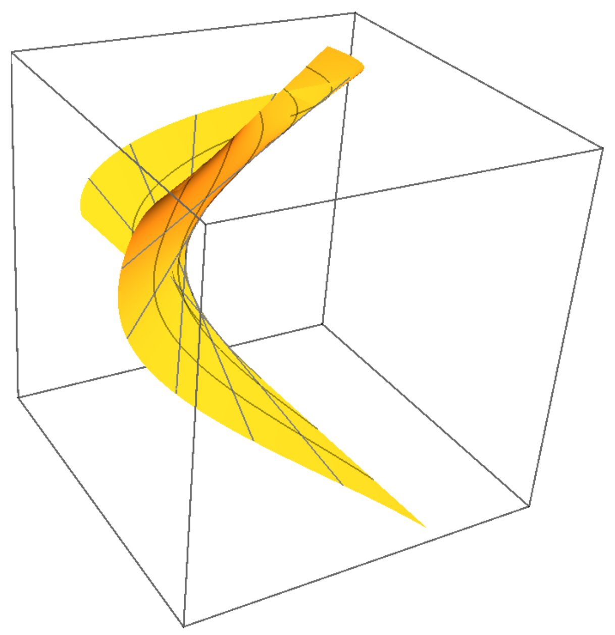
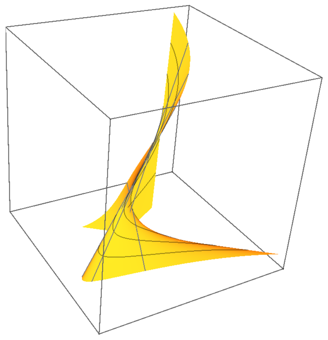
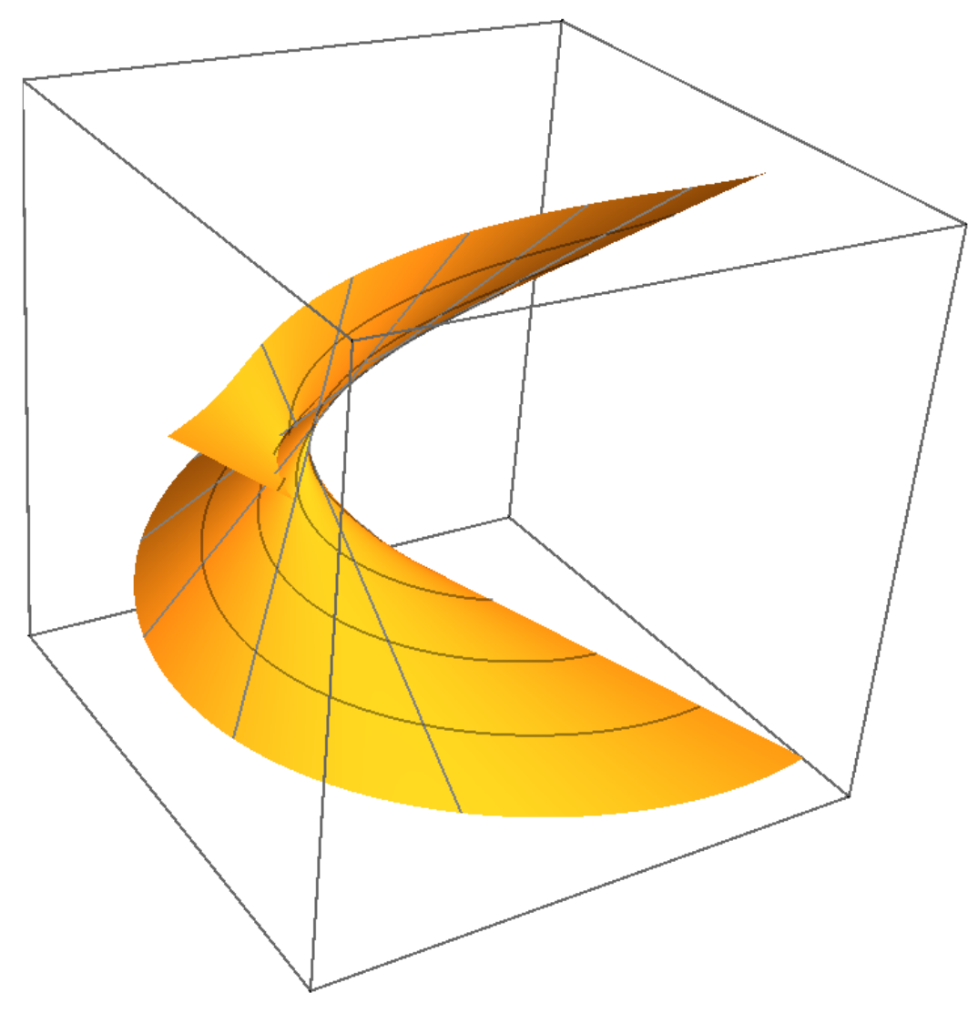
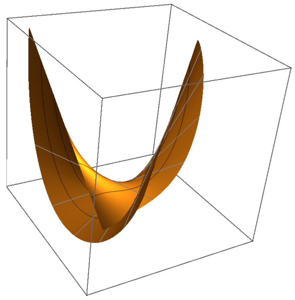
• $C(2,3,4)=\{(x_1,x_2,x_3)\mid x_1=u^2,x_2=u^3,x_3=u^4\}$ (Figure 2);
  

  Figure 2. $C(2,3,4)$.
• $C(2,3,4,5)=\{(x_1,x_2,x_3,x_4)\mid x_1=u^2,x_2=u^3,x_3=u^4,x_4=u^5\}$ (Figure 3);
  

  Figure 3. The projection of $C(2,3,4,5)$ on 3-space.
• $C(2,3)\times \mathbb{R}=\{(x_1,x_2)\mid x_1=u^2,x_2=u^3\}\times \mathbb{R}$ (Figure 4);
  

  Figure 4. $C(2,3)\times \mathbb{R}$.
• $SW=\{(x_1,x_2,x_3)\mid x_1=3u^4+u^{2}v,x_2=4u^3+2uv,x_3=v\}$ (Figure 5);
  

  Figure 5. SW.
• $BF=\{(x_1,x_2,x_3,x_4)\mid x_1=5u^4+3v{u}^2+2wu,x_2=4u^5+2v{u}^3+w{u}^2,x_3=u$, $x_4=v\}$ (Figure 6);
  

  Figure 6. The projection of $BF$ on 3-space.
• $C\left(BF\right)=\{(x_1,x_2,x_3,x_4)\mid x_1=6u^5+u^{3}v,x_2=25u^4+9u^{2}v,x_3=10u^3+3uv$, $x_4=v\}$ (Figure 7).
  

  Figure 7. The projection of $C\left(BF\right)$ on 3-space.

The proof of Theorem 1 will be placed at the end of the fourth section.

3. Singularities of Type $A_k$

This section establishes the relationship between the singularity types of volumetric distance functions and the contact geometry of null Cartan curves with lightlike hyperplanes. We analyze $A_k$-singularities through successive derivative conditions of the distance function $g_{\mathit{x}}\left(t\right)$, which encode geometric constraints on the curve’s interaction with its null Cartan frame. The technical tool Proposition 3 provides a complete characterization of singularity orders via explicit parametrizations of contact points, directly linking jet conditions to curvature invariants and the fundamental invariant $\sigma \left(t\right)$.

Let $F:(\mathbb{R}\times {\mathbb{R}}^r,(t_0,{\mathit{x}}_0))\to \mathbb{R}$ be a smooth function germ. We call F an r-parameter unfolding of f, where $f\left(t\right)=F_{{\mathit{x}}_0}(t,{\mathit{x}}_0)$. We say f has

(1)

$A_k$-singularity at $t_0$ if $f^{\left(p\right)}\left(t_0\right)=0(\forall 1\le p\le k)$ and $f^{(k+1)}\left(t_0\right)\ne 0$;

(2)

$A_{\ge k}$-singularity if $f^{\left(p\right)}\left(t_0\right)=0(\forall 1\le p\le k)$.

For a null Cartan curve $\mathit{\beta }:I\to {\mathbb{R}}_1^4$ with ${\kappa }_1\left(t\right)\psi \left(t\right)\ne 0$, define the volumetric distance function:

$$G(t,\mathit{x})=⟨\mathit{x}-\mathit{\beta }\left(t\right),\mathit{\lambda }\left(t\right)⟩$$

where $g_{\mathit{x}}\left(t\right)=G(t,\mathit{x})$. This function characterizes geometric relations between points and the curve’s frame.

Proposition 3.

Let $\mathit{\beta }:I\to {\mathbb{R}}_1^4$ be a null Cartan curve with ${\kappa }_1\left(t\right)\psi \left(t\right)\ne 0$. Then, the following hold:

(1)

$g_{\mathit{x}}\left(t\right)=0$ if and only if there exist $\mu ,\eta ,\nu \in \mathbb{R}$ such that

$$\mathit{x}=\mathit{\beta }\left(t\right)+\eta \mathit{\lambda }\left(t\right)+\nu {\mathit{w}}_1\left(t\right)+\mu {\mathit{w}}_2\left(t\right).$$

(2)

$g_{\mathit{x}}\left(t\right)=g_{\mathit{x}}^{\prime }\left(t\right)=0$ if and only if there exist $\mu ,\eta \in \mathbb{R}$ such that

$$\mathit{x}=\mathit{\beta }\left(t\right)+\frac{a}{{\kappa }_1}\left(t\right){\mathit{w}}_1\left(t\right)+\eta \mathit{\lambda }\left(t\right)+\mu \left(-\frac{{\kappa }_2}{{\kappa }_1}\left(t\right){\mathit{w}}_1\left(t\right)+{\mathit{w}}_2\left(t\right)\right).$$

(3)

$g_{\mathit{x}}\left(t\right)=g_{\mathit{x}}^{\prime }\left(t\right)=g_{\mathit{x}}^{″}\left(t\right)=0$ if and only if there exists $m\in \mathbb{R}$ such that

$$\begin{array}{c}\hfill \mathit{x}=\mathit{\beta }\left(t\right)+\frac{a}{{\kappa }_1}{\mathit{w}}_1\left(t\right)+\frac{a{\kappa }_1^{\prime }-a^{\prime }{\kappa }_1}{{\kappa }_{1}D}\left(t\right)\mathit{\lambda }\left(t\right)+\mu \left(\frac{\Delta \kappa }{{\kappa }_{1}D}\mathit{\lambda }-\frac{{\kappa }_2}{{\kappa }_1}{\mathit{w}}_1+{\mathit{w}}_2\right)\left(t\right).\end{array}$$

(4)

$g_{\mathit{x}}\left(t\right)=g_{\mathit{x}}^{\prime }\left(t\right)=g_{\mathit{x}}^{″}\left(t\right)=g_{\mathit{x}}^{‴}\left(t\right)=0$ if and only if

$$\begin{array}{c}\hfill \mathit{x}=\mathit{\beta }\left(t\right)+\frac{a}{{\kappa }_1}{\mathit{w}}_1\left(t\right)+\frac{a{\kappa }_1^{\prime }-a^{\prime }{\kappa }_1}{{\kappa }_{1}D}\left(t\right)\mathit{\lambda }\left(t\right)+\tilde{\mu }\left(\frac{\Delta \kappa }{{\kappa }_{1}D}\mathit{\lambda }-\frac{{\kappa }_2}{{\kappa }_1}{\mathit{w}}_1+{\mathit{w}}_2\right)\left(t\right).\end{array}$$

(5)

$g_{\mathit{x}}\left(t\right)=g_{\mathit{x}}^{\prime }\left(t\right)=g_{\mathit{x}}^{″}\left(t\right)=g_{\mathit{x}}^{‴}\left(t\right)=g_{\mathit{x}}^{\left(4\right)}\left(t\right)=0$ if and only if $\sigma \left(t\right)=0$ and

$$\begin{array}{c}\hfill \mathit{x}=\mathit{\beta }\left(t\right)+\frac{a}{{\kappa }_1}{\mathit{w}}_1\left(t\right)+\frac{a{\kappa }_1^{\prime }-a^{\prime }{\kappa }_1}{{\kappa }_{1}D}\left(t\right)\mathit{\lambda }\left(t\right)+\tilde{\mu }\left(\frac{\Delta \kappa }{{\kappa }_{1}D}\mathit{\lambda }-\frac{{\kappa }_2}{{\kappa }_1}{\mathit{w}}_1+{\mathit{w}}_2\right)\left(t\right).\end{array}$$

(6)

$g_{\mathit{x}}\left(t\right)=g_{\mathit{x}}^{\prime }\left(t\right)=g_{\mathit{x}}^{″}\left(t\right)=g_{\mathit{x}}^{‴}\left(t\right)=g_{\mathit{x}}^{\left(4\right)}\left(t\right)=g_{\mathit{x}}^{\left(5\right)}\left(t\right)=0$ if and only if $\sigma \left(t\right)={\sigma }^{\prime }\left(t\right)=0$ and

$$\begin{array}{c}\hfill \mathit{x}=\mathit{\beta }\left(t\right)+\frac{a}{{\kappa }_1}{\mathit{w}}_1\left(t\right)+\frac{a{\kappa }_1^{\prime }-a^{\prime }{\kappa }_1}{{\kappa }_{1}D}\left(t\right)\mathit{\lambda }\left(t\right)+\tilde{\mu }\left(\frac{\Delta \kappa }{{\kappa }_{1}D}\mathit{\lambda }-\frac{{\kappa }_2}{{\kappa }_1}{\mathit{w}}_1+{\mathit{w}}_2\right)\left(t\right).\end{array}$$

Proof. (1) Observing that $\{\mathit{\xi },\mathit{\lambda },{\mathit{w}}_1,{\mathit{w}}_2\}$ forms a frame along $\mathit{\beta }$, there exist real numbers $\mu ,\nu ,\eta ,\delta \in \mathbb{R}$ such that

$$\mathit{x}-\mathit{\beta }\left(t\right)=\nu \mathit{\xi }\left(t\right)+\eta \mathit{\lambda }\left(t\right)+\delta {\mathit{w}}_1\left(t\right)+\mu {\mathit{w}}_2\left(t\right).$$

This leads to the following result:

$$\begin{array}{cc}\hfill g_{\mathit{x}}\left(t\right)& =⟨\mathit{x}-\mathit{\beta }\left(t\right),\mathit{\lambda }\left(t\right)⟩\hfill \\ \hfill & =⟨\nu \mathit{\xi }\left(t\right)+\eta \mathit{\lambda }\left(t\right)+\delta {\mathit{w}}_1\left(t\right)+\mu {\mathit{w}}_2\left(t\right),\mathit{\lambda }\left(t\right)⟩\hfill \\ \hfill & =\nu ,\hfill \end{array}$$

because $g_{\mathit{x}}\left(t\right)=0$, so we have $\nu =0$; we obtain

$$\begin{array}{c}\hfill \mathit{x}-\mathit{\beta }\left(t\right)=\eta \mathit{\lambda }\left(t\right)+\delta {\mathit{w}}_1\left(t\right)+\mu {\mathit{w}}_2\left(t\right).\end{array}$$

The first assertion is established.

(2)

Under the condition $g_{\mathit{x}}\left(t\right)=0$, we obtain

$$\begin{array}{cc}\hfill g_{\mathit{x}}^{\prime }\left(t\right)& ={⟨\mathit{x}-\mathit{\beta }\left(t\right),\mathit{\lambda }\left(t\right)⟩}^{\prime }\hfill \\ \hfill & =-⟨a\left(t\right)\mathit{\xi }\left(t\right),\mathit{\lambda }\left(t\right)⟩+⟨\mathit{x}-\mathit{\beta }\left(t\right),{\kappa }_1\left(t\right){\mathit{w}}_1\left(t\right)+{\kappa }_2\left(t\right){\mathit{w}}_2\left(t\right)⟩\hfill \\ \hfill & =-a\left(t\right)+{\kappa }_1\left(t\right)\delta +{\kappa }_2\left(t\right)\mu ,\hfill \end{array}$$

which shows that $g_{\mathit{x}}\left(t\right)=g_{\mathit{x}}^{\prime }\left(t\right)=0$ is equivalent to $\delta =\frac{a\left(t\right)-{\kappa }_2\left(t\right)\mu }{{\kappa }_1\left(t\right)}$. Consequently,

$$\begin{array}{c}\hfill \mathit{x}-\mathit{\beta }\left(t\right)=\eta \mathit{\lambda }\left(t\right)+\frac{a\left(t\right)-{\kappa }_2\left(t\right)\mu }{{\kappa }_1\left(t\right)}{\mathit{w}}_1\left(t\right)+\mu {\mathit{w}}_2\left(t\right),\end{array}$$

thereby confirming assertion (2).

(3)

Starting from $g_{\mathit{x}}\left(t\right)=g_{\mathit{x}}^{\prime }\left(t\right)=0$, we compute

$$\begin{array}{cc}\hfill g_{\mathit{x}}^{″}\left(t\right)=& -a^{\prime }\left(t\right)+{⟨\mathit{x}-\mathit{\beta }\left(t\right),{\kappa }_1\left(t\right){\mathit{w}}_1\left(t\right)+{\kappa }_2\left(t\right){\mathit{w}}_2\left(t\right)⟩}^{\prime }\hfill \\ \hfill =& -a^{\prime }\left(t\right)-⟨a\left(t\right)\mathit{\xi }\left(t\right),{\kappa }_1\left(t\right){\mathit{w}}_1\left(t\right)+{\kappa }_2\left(t\right){\mathit{w}}_2\left(t\right)⟩+⟨\mathit{x}-\mathit{\beta }\left(t\right),{\left({\kappa }_1\left(t\right){\mathit{w}}_1\left(t\right)+{\kappa }_2\left(t\right){\mathit{w}}_2\left(t\right)\right)}^{\prime }⟩\hfill \\ \hfill =& -a^{\prime }\left(t\right)+⟨\eta \mathit{\lambda }\left(t\right)+\frac{a\left(t\right)-{\kappa }_2\left(t\right)\mu }{{\kappa }_1\left(t\right)}{\mathit{w}}_1\left(t\right)+\mu {\mathit{w}}_2\left(t\right),{\kappa }_1^{\prime }\left(t\right){\mathit{w}}_1\left(t\right)+{\kappa }_2^{\prime }\left(t\right){\mathit{w}}_2\left(t\right)\hfill \\ \hfill & -D\left(t\right)\mathit{\xi }\left(t\right)-{\kappa }_1\left(t\right)\mathit{\lambda }\left(t\right)⟩\hfill \\ \hfill =& -a^{\prime }\left(t\right)-D\left(t\right)\eta +\frac{a\left(t\right)-{\kappa }_2\left(t\right)\mu }{{\kappa }_1\left(t\right)}{\kappa }_1^{\prime }\left(t\right)+\mu {\kappa }_2^{\prime }\left(t\right).\hfill \end{array}$$

Thus, $g_{\mathit{x}}\left(t\right)=g_{\mathit{x}}^{\prime }\left(t\right)=g_{\mathit{x}}^{″}\left(t\right)=0$ is satisfied precisely when

$$\eta =\frac{a\left(t\right){\kappa }_1^{\prime }\left(t\right)-a^{\prime }\left(t\right){\kappa }_1\left(t\right)+\mu \Delta \kappa \left(t\right)}{{\kappa }_1\left(t\right)D\left(t\right)},$$

which implies

$$\begin{array}{c}\hfill \mathit{x}=\mathit{\beta }\left(t\right)+\frac{a}{{\kappa }_1}{\mathit{w}}_1+\frac{a{\kappa }_1^{\prime }-a^{\prime }{\kappa }_1}{{\kappa }_{1}D}\mathit{\lambda }+\mu \left(\frac{\Delta \kappa }{{\kappa }_{1}D}\mathit{\lambda }-\frac{{\kappa }_2}{{\kappa }_1}{\mathit{w}}_1+{\mathit{w}}_2\right),\end{array}$$

thereby establishing assertion (3).

(4)

Assuming $g_{\mathit{x}}\left(t\right)=g_{\mathit{x}}^{\prime }\left(t\right)=g_{\mathit{x}}^{″}\left(t\right)=0$, we calculate

$$\begin{array}{cc}\hfill g_{\mathit{x}}^{‴}\left(t\right)=& {\left(-a^{\prime }\left(t\right)+⟨\mathit{x}-\mathit{\beta }\left(t\right),{\kappa }_1^{\prime }\left(t\right){\mathit{w}}_1\left(t\right)+{\kappa }_2^{\prime }\left(t\right){\mathit{w}}_2\left(t\right)-D\left(t\right)\mathit{\xi }\left(t\right)-{\kappa }_1\left(t\right)\mathit{\lambda }\left(t\right)⟩\right)}^{\prime }\hfill \\ \hfill =& -a^{″}\left(t\right)+⟨-a\left(t\right)\mathit{\xi }\left(t\right),{\kappa }_1^{\prime }\left(t\right){\mathit{w}}_1\left(t\right)+{\kappa }_2^{\prime }\left(t\right){\mathit{w}}_2\left(t\right)-D\left(t\right)\mathit{\xi }\left(t\right)-{\kappa }_1\left(t\right)\mathit{\lambda }\left(t\right)⟩\hfill \\ \hfill & +⟨\mathit{x}-\mathit{\beta }\left(t\right),{\left({\kappa }_1^{\prime }\left(t\right){\mathit{w}}_1\left(t\right)+{\kappa }_2^{\prime }\left(t\right){\mathit{w}}_2\left(t\right)-({\kappa }_1^2\left(t\right)+{\kappa }_2^2\left(t\right))\mathit{\xi }\left(t\right)-{\kappa }_1\left(t\right)\mathit{\lambda }\left(t\right)\right)}^{\prime }⟩\hfill \\ \hfill =& -a^{″}\left(t\right)+a\left(t\right){\kappa }_1\left(t\right)+⟨\frac{a}{{\kappa }_1}\left(t\right){\mathit{w}}_1\left(t\right)+\frac{a\left(t\right){\kappa }_1^{\prime }\left(t\right)-a^{\prime }\left(t\right){\kappa }_1\left(t\right)}{{\kappa }_1\left(t\right)D\left(t\right)}\mathit{\lambda }\left(t\right)\hfill \\ \hfill & +\mu \left(\frac{\Delta \kappa \left(t\right)}{{\kappa }_{1}D\left(t\right)}\mathit{\lambda }\left(t\right)-\frac{{\kappa }_2}{{\kappa }_1}\left(t\right){\mathit{w}}_1\left(t\right)+{\mathit{w}}_2\left(t\right)\right),\mathit{\xi }\left(t\right)(-3{\kappa }_1\left(t\right){\kappa }_1^{\prime }\left(t\right)-3{\kappa }_2\left(t\right){\kappa }_2^{\prime }\left(t\right))\hfill \\ \hfill & -2{\kappa }_1^{\prime }\left(t\right)\mathit{\lambda }\left(t\right)+{\mathit{w}}_1\left(t\right)({\kappa }_1^{″}\left(t\right)-2{\kappa }_1(t{)}^2-{\kappa }_2(t{)}^2)+{\mathit{w}}_2\left(t\right)({\kappa }_2^{″}\left(t\right)-{\kappa }_1\left(t\right){\kappa }_2\left(t\right))⟩\hfill \\ \hfill =& -a^{″}\left(t\right)+a\left(t\right){\kappa }_1\left(t\right)+(\frac{a}{{\kappa }_1}\left(t\right)-\mu \frac{{\kappa }_2}{{\kappa }_1}\left(t\right))({\kappa }_1^{″}\left(t\right)-2{\kappa }_1^2\left(t\right)-{\kappa }_2(t{)}^2)+({\kappa }_2^{″}\left(t\right)\hfill \\ \hfill & -{\kappa }_1\left(t\right){\kappa }_2\left(t\right))\mu +\left(\frac{a\left(t\right){\kappa }_1^{\prime }\left(t\right)-a^{\prime }\left(t\right){\kappa }_1\left(t\right)}{{\kappa }_1\left(t\right)D\left(t\right)}+\mu \frac{\Delta \kappa \left(t\right)}{{\kappa }_{1}D\left(t\right)}\right)(-3{\kappa }_1\left(t\right){\kappa }_1^{\prime }\left(t\right)-3{\kappa }_2\left(t\right){\kappa }_2^{\prime }\left(t\right)).\hfill \end{array}$$

Using $g_{\mathit{x}}\left(t\right)=g_{\mathit{x}}^{\prime }\left(t\right)=g_{\mathit{x}}^{″}\left(t\right)=g_{\mathit{x}}^{‴}\left(t\right)=0$, we obtain

$$\begin{array}{cc}\hfill \mu & =\frac{D({\kappa }_1{a}^{″}-a{\kappa }_1^{″})+3({\kappa }_1{\kappa }_1^{\prime }+{\kappa }_2{\kappa }_2^{\prime })(a{\kappa }_1^{\prime }-{\kappa }_1{a}^{\prime })+a{D}^2}{D({\kappa }_1{\kappa }_2^{″}-{\kappa }_2{\kappa }_1^{″})+3({\kappa }_1{\kappa }_1^{\prime }+{\kappa }_2{\kappa }_2^{\prime })({\kappa }_2{\kappa }_1^{\prime }-{\kappa }_1{\kappa }_2^{\prime })+{\kappa }_2{D}^2}\left(t\right)\hfill \\ \hfill & =\tilde{\mu }\left(t\right),\hfill \end{array}$$

which implies

$$\begin{array}{c}\hfill \mathit{x}=\mathit{\beta }\left(t\right)+\frac{a}{{\kappa }_1}{\mathit{w}}_1\left(t\right)+\frac{a{\kappa }_1^{\prime }-a^{\prime }{\kappa }_1}{{\kappa }_{1}D}\left(t\right)\mathit{\lambda }\left(t\right)+\tilde{\mu }\left(\frac{\Delta \kappa }{{\kappa }_{1}D}\mathit{\lambda }-\frac{{\kappa }_2}{{\kappa }_1}{\mathit{w}}_1+{\mathit{w}}_2\right)\left(t\right),\end{array}$$

thus proving assertion (4).

(5)

From $g_{\mathit{x}}\left(t\right)=g_{\mathit{x}}^{\prime }\left(t\right)=g_{\mathit{x}}^{″}\left(t\right)=g_{\mathit{x}}^{‴}\left(t\right)=0$, we derive

$$\begin{array}{cc}\hfill g_{\mathit{x}}^{\left(4\right)}\left(t\right)=& -a^{‴}\left(t\right)+a^{\prime }\left(t\right){\kappa }_1\left(t\right)+a\left(t\right){\kappa }_1^{\prime }\left(t\right)+(⟨\mathit{x}-\mathit{\beta }\left(t\right),\mathit{\xi }\left(t\right)(-3{\kappa }_1\left(t\right){\kappa }_1^{\prime }\left(t\right)-3{\kappa }_2\left(t\right){\kappa }_2^{\prime }\left(t\right))\hfill \\ \hfill & -2{\kappa }_1^{\prime }\left(t\right)\mathit{\lambda }\left(t\right)+{\mathit{w}}_1\left(t\right)({\kappa }_1^{″}\left(t\right)-2{\kappa }_1(t{)}^2-{\kappa }_2(t{)}^2)+{\mathit{w}}_2\left(t\right)({\kappa }_2^{″}\left(t\right)-{\kappa }_1\left(t\right){\kappa }_2\left(t\right))⟩{)}^{\prime }\hfill \\ \hfill =& -a^{‴}\left(t\right)+a^{\prime }\left(t\right){\kappa }_1\left(t\right)+a\left(t\right){\kappa }_1^{\prime }\left(t\right)+⟨-a\left(t\right)\mathit{\xi }\left(t\right),\mathit{\xi }\left(t\right)(-3{\kappa }_1\left(t\right){\kappa }_1^{\prime }\left(t\right)-3{\kappa }_2\left(t\right){\kappa }_2^{\prime }\left(t\right))\hfill \\ \hfill & -2{\kappa }_1^{\prime }\left(t\right)\mathit{\lambda }\left(t\right)+{\mathit{w}}_1\left(t\right)({\kappa }_1^{″}\left(t\right)-2{\kappa }_1^2\left(t\right)-{\kappa }_2^2\left(t\right))+{\mathit{w}}_2\left(t\right)({\kappa }_2^{″}\left(t\right)-{\kappa }_1\left(t\right){\kappa }_2\left(t\right))⟩\hfill \\ \hfill =& -a^{‴}\left(t\right)+a^{\prime }\left(t\right){\kappa }_1\left(t\right)-a\left(t\right){\kappa }_1^{\prime }\left(t\right)+⟨\frac{a}{{\kappa }_1}\left(t\right){\mathit{w}}_1\left(t\right)+\frac{a\left(t\right){\kappa }_1^{\prime }\left(t\right)-a^{\prime }\left(t\right){\kappa }_1\left(t\right)}{{\kappa }_1\left(t\right)D\left(t\right)}\mathit{\lambda }\left(t\right)\hfill \\ \hfill & +\tilde{\mu }\left(t\right)\left(\frac{\Delta \kappa \left(t\right)}{{\kappa }_{1}D\left(t\right)}\mathit{\lambda }\left(t\right)-\frac{{\kappa }_2}{{\kappa }_1}\left(t\right){\mathit{w}}_1\left(t\right)+{\mathit{w}}_2\left(t\right)\right),\mathit{\xi }\left(t\right)(-3{\left({\kappa }_1^{\prime }\left(t\right)\right)}^2\hfill \\ \hfill & -3{\left({\kappa }_2^{\prime }\left(t\right)\right)}^2-3{\kappa }_1\left(t\right){\kappa }_1^{″}\left(t\right)-{\kappa }_1\left(t\right)({\kappa }_1^{″}\left(t\right)-2{\kappa }_1^2\left(t\right)-{\kappa }_2^2\left(t\right))-3{\kappa }_2\left(t\right){\kappa }_2^{″}\left(t\right)\hfill \\ \hfill & -{\kappa }_2\left(t\right)({\kappa }_2^{″}\left(t\right)-{\kappa }_1\left(t\right){\kappa }_2\left(t\right)))+{\mathit{w}}_1\left(t\right)(-9{\kappa }_1\left(t\right){\kappa }_1^{\prime }\left(t\right)-5{\kappa }_2\left(t\right){\kappa }_2^{\prime }\left(t\right)+{\kappa }_1{(}^{3)}\left(t\right))\hfill \\ \hfill & +\mathit{\lambda }\left(t\right)(-3{\kappa }_1^{″}\left(t\right)+2{\kappa }_1^2\left(t\right)+{\kappa }_2(t{)}^2)+{\mathit{w}}_2\left(t\right)(-3{\kappa }_2\left(t\right){\kappa }_1^{\prime }\left(t\right)-{\kappa }_1\left(t\right){\kappa }_2^{\prime }\left(t\right)+{\kappa }_2{(}^{3)}\left(t\right))⟩\hfill \\ \hfill =& -a^{‴}\left(t\right)+\frac{\mathcal{N}\left(t\right)}{\mathcal{K}\left(t\right)}.\hfill \end{array}$$

It follows that $g_{\mathit{x}}\left(t\right)=g_{\mathit{x}}^{\prime }\left(t\right)=g_{\mathit{x}}^{″}\left(t\right)=g_{\mathit{x}}^{‴}\left(t\right)=g_{\mathit{x}}^{\left(4\right)}\left(t\right)=0$ holds precisely when

$$\begin{array}{c}\hfill \mathit{x}=\mathit{\beta }\left(t\right)+\frac{a}{{\kappa }_1}{\mathit{w}}_1\left(t\right)+\frac{a{\kappa }_1^{\prime }-a^{\prime }{\kappa }_1}{{\kappa }_{1}D}\left(t\right)\mathit{\lambda }\left(t\right)+\tilde{\mu }\left(\frac{\Delta \kappa }{{\kappa }_{1}D}\mathit{\lambda }-\frac{{\kappa }_2}{{\kappa }_1}{\mathit{w}}_1+{\mathit{w}}_2\right)\left(t\right).\end{array}$$

and

$$\begin{array}{cc}\hfill \sigma \left(t\right)=& -a^{\left(3\right)}\left(t\right)+\frac{\mathcal{N}\left(t\right)}{\mathcal{K}\left(t\right)}=0.\hfill \end{array}$$

This verifies assertion (5).

(6)

Assuming $g_{\mathit{x}}\left(t\right)=g_{\mathit{x}}^{\prime }\left(t\right)=g_{\mathit{x}}^{″}\left(t\right)=g_{\mathit{x}}^{‴}\left(t\right)=g_{\mathit{x}}^{\left(4\right)}\left(t\right)=0$, we compute

$$\begin{array}{cc}\hfill g_{\mathit{x}}^{\left(5\right)}\left(t\right)=& (-a^{‴}\left(t\right)+a^{\prime }\left(t\right){\kappa }_1\left(t\right)-a\left(t\right){\kappa }_1^{\prime }\left(t\right)+⟨\mathit{x}-\mathit{\beta }\left(t\right),\mathit{\xi }\left(t\right)(-3{\left({\kappa }_1^{\prime }\left(t\right)\right)}^2\hfill \\ \hfill & -3{\left({\kappa }_2^{\prime }\left(t\right)\right)}^2-3{\kappa }_1\left(t\right){\kappa }_1^{″}\left(t\right)-{\kappa }_1\left(t\right)({\kappa }_1^{″}\left(t\right)-2{\kappa }_1^2\left(t\right)-{\kappa }_2^2\left(t\right))-3{\kappa }_2\left(t\right){\kappa }_2^{″}\left(t\right)\hfill \\ \hfill & -{\kappa }_2\left(t\right)({\kappa }_2^{″}\left(t\right)-{\kappa }_1\left(t\right){\kappa }_2\left(t\right)))+{\mathit{w}}_1\left(t\right)(-9{\kappa }_1\left(t\right){\kappa }_1^{\prime }\left(t\right)-5{\kappa }_2\left(t\right){\kappa }_2^{\prime }\left(t\right)+{\kappa }_1^{\left(3\right)}\left(t\right))\hfill \\ \hfill & +\mathit{\lambda }\left(t\right)(-3{\kappa }_1^{″}\left(t\right)+2{\kappa }_1^2\left(t\right)+{\kappa }_2^2\left(t\right))+{\mathit{w}}_2\left(t\right)(-3{\kappa }_2\left(t\right){\kappa }_1^{\prime }\left(t\right)-{\kappa }_1\left(t\right){\kappa }_2^{\prime }\left(t\right)+{\kappa }_2^{\left(3\right)}\left(t\right))⟩{)}^{\prime }\hfill \\ \hfill =& -a^{\left(4\right)}\left(t\right)+a^{″}\left(t\right){\kappa }_1\left(t\right)-a\left(t\right){\kappa }_1^{″}\left(t\right)+⟨-a\left(t\right)\mathit{\xi }\left(t\right),\mathit{\lambda }\left(t\right)(-3{\kappa }_1^{″}\left(t\right)+2{\kappa }_1^2\left(t\right)+{\kappa }_2^2\left(t\right))⟩\hfill \\ \hfill =& -a^{\left(4\right)}\left(t\right)+a^{″}\left(t\right){\kappa }_1\left(t\right)-a\left(t\right){\kappa }_1^{″}\left(t\right)+⟨\frac{a}{{\kappa }_1}\left(t\right){\mathit{w}}_1\left(t\right)+\frac{a\left(t\right){\kappa }_1^{\prime }\left(t\right)-a^{\prime }\left(t\right){\kappa }_1\left(t\right)}{{\kappa }_1\left(t\right)D\left(t\right)}\mathit{\lambda }\left(t\right)\hfill \\ \hfill & +\tilde{\mu }\left(t\right)\left(\frac{\Delta \kappa \left(t\right)}{{\kappa }_{1}D\left(t\right)}\mathit{\lambda }\left(t\right)-\frac{{\kappa }_2}{{\kappa }_1}\left(t\right){\mathit{w}}_1\left(t\right)+{\mathit{w}}_2\left(t\right)\right),\left(\mathit{\xi }\left(t\right)\right(-3{\left({\kappa }_1^{\prime }\left(t\right)\right)}^2\hfill \\ \hfill & -3{\left({\kappa }_2^{\prime }\left(t\right)\right)}^2-3{\kappa }_1\left(t\right){\kappa }_1^{″}\left(t\right)-{\kappa }_1\left(t\right)({\kappa }_1^{″}\left(t\right)-2{\kappa }_1^2\left(t\right)-{\kappa }_2^2\left(t\right))-3{\kappa }_2\left(t\right){\kappa }_2^{″}\left(t\right)\hfill \\ \hfill & -{\kappa }_2\left(t\right)({\kappa }_2^{″}\left(t\right)-{\kappa }_1\left(t\right){\kappa }_2\left(t\right)))+{\mathit{w}}_1\left(t\right)(-9{\kappa }_1\left(t\right){\kappa }_1^{\prime }\left(t\right)-5{\kappa }_2\left(t\right){\kappa }_2^{\prime }\left(t\right)+{\kappa }_1^{\left(3\right)}\left(t\right))\hfill \\ \hfill & +\mathit{\lambda }\left(t\right)(-3{\kappa }_1^{″}\left(t\right)+2{\kappa }_1^2\left(t\right)+{\kappa }_2^2\left(t\right))+{\mathit{w}}_2\left(t\right)(-3{\kappa }_2\left(t\right){\kappa }_1^{\prime }\left(t\right)-{\kappa }_1\left(t\right){\kappa }_2^{\prime }\left(t\right)+{\kappa }_2^{\left(3\right)}\left(t\right)){)}^{\prime }⟩\hfill \\ \hfill =& {\sigma }^{\prime }\left(t\right).\hfill \end{array}$$

Thus, $g_{\mathit{x}}\left(t\right)=g_{\mathit{x}}^{\prime }\left(t\right)=g_{\mathit{x}}^{″}\left(t\right)=g_{\mathit{x}}^{‴}\left(t\right)=g_{\mathit{x}}^{\left(4\right)}\left(t\right)=g_{\mathit{x}}^{\left(5\right)}\left(t\right)=0$ holds precisely when

$$\begin{array}{c}\hfill \mathit{x}=\mathit{\beta }\left(t\right)+\frac{a}{{\kappa }_1}{\mathit{w}}_1\left(t\right)+\frac{a{\kappa }_1^{\prime }-a^{\prime }{\kappa }_1}{{\kappa }_{1}D}\left(t\right)\mathit{\lambda }\left(t\right)+\tilde{\mu }\left(\frac{\Delta \kappa }{{\kappa }_{1}D}\mathit{\lambda }-\frac{{\kappa }_2}{{\kappa }_1}{\mathit{w}}_1+{\mathit{w}}_2\right)\left(t\right).\end{array}$$

$\sigma \left(t\right)=0$, and ${\sigma }^{\prime }\left(t\right)=0$, thereby confirming assertion (6). □

Based on Proposition 3, the following corollary can be directly obtained.

Corollary 1.

Let $\mathit{\beta }:I\to {\mathbb{R}}_1^4$ be a null Cartan curve satisfying ${\kappa }_1\left(t\right)\psi \left(t\right)\ne 0$. Then, the following holds:

(1)

The function $g_{\mathit{x}}$ exhibits an $A_1$-singularity at $t_0$ if and only if there exist $\mu ,\eta \in \mathbb{R}$ such that

$$\eta \ne \frac{a\left(t_0\right){\kappa }_1^{\prime }\left(t_0\right)-a^{\prime }\left(t_0\right){\kappa }_1\left(t_0\right)+\mu \Delta \kappa \left(t_0\right)}{{\kappa }_1\left(t_0\right)D\left(t_0\right)}$$

and

$$\mathit{x}=\mathit{\beta }\left(t_0\right)+\frac{a}{{\kappa }_1}\left(t_0\right){\mathit{w}}_1\left(t_0\right)+\eta \mathit{\lambda }\left(t_0\right)+\mu \left(-\frac{{\kappa }_2}{{\kappa }_1}\left(t_0\right){\mathit{w}}_1\left(t_0\right)+{\mathit{w}}_2\left(t_0\right)\right).$$

Under this condition, $\mathit{\beta }$ and $H{S}_{t_0}^L(\mathit{\lambda }\left(t_0\right),⟨\mathit{\beta }\left(t_0\right),\mathit{\lambda }\left(t_0\right)⟩)$ exhibit two-point contact at $t=t_0$.

(2)

The function $g_{\mathit{x}}$ exhibits an $A_2$-singularity at $t_0$ if and only if there exists $\mu \in \mathbb{R}$ satisfying

$$\mu \ne \tilde{\mu }\left(t_0\right),$$

and

$$\begin{array}{c}\hfill \mathit{x}=\mathit{\beta }\left(t_0\right)+\frac{a}{{\kappa }_1}{\mathit{w}}_1\left(t_0\right)+\frac{a{\kappa }_1^{\prime }-a^{\prime }{\kappa }_1}{{\kappa }_{1}D}\left(t\right)\mathit{\lambda }\left(t_0\right)+\mu \left(\frac{\Delta \kappa }{{\kappa }_{1}D}\mathit{\lambda }-\frac{{\kappa }_2}{{\kappa }_1}{\mathit{w}}_1+{\mathit{w}}_2\right)\left(t_0\right).\end{array}$$

Under this condition, $\mathit{\beta }$ and $H{S}_{t_0}^L(\mathit{\lambda }\left(t_0\right),⟨\mathit{\beta }\left(t_0\right),\mathit{\lambda }\left(t_0\right)⟩)$ exhibit three-point contact at $t=t_0$.

(3)

The function $g_{\mathit{x}}$ displays an $A_3$-singularity at $t_0$ if and only if $\sigma \left(t_0\right)\ne 0$ and

$$\begin{array}{c}\hfill \mathit{x}=\mathit{\beta }\left(t_0\right)+\frac{a}{{\kappa }_1}{\mathit{w}}_1\left(t_0\right)+\frac{a{\kappa }_1^{\prime }-a^{\prime }{\kappa }_1}{{\kappa }_{1}D}\left(t_0\right)\mathit{\lambda }\left(t_0\right)+\tilde{\mu }\left(\frac{\Delta \kappa }{{\kappa }_{1}D}\mathit{\lambda }-\frac{{\kappa }_2}{{\kappa }_1}{\mathit{w}}_1+{\mathit{w}}_2\right)\left(t_0\right).\end{array}$$

Under this condition, $\mathit{\beta }$ and $H{S}_{t_0}^L(\mathit{\lambda }\left(t_0\right),⟨\mathit{\beta }\left(t_0\right),\mathit{\lambda }\left(t_0\right)⟩)$ exhibit four-point contact at $t=t_0$.

(4)

The function $g_{\mathit{x}}$ possesses an $A_4$-singularity at $t_0$ if and only if $\sigma \left(t_0\right)=0$, ${\sigma }^{\prime }\left(t_0\right)\ne 0$, and

$$\begin{array}{c}\hfill \mathit{x}=\mathit{\beta }\left(t_0\right)+\frac{a}{{\kappa }_1}{\mathit{w}}_1\left(t_0\right)+\frac{a{\kappa }_1^{\prime }-a^{\prime }{\kappa }_1}{{\kappa }_{1}D}\left(t_0\right)\mathit{\lambda }\left(t_0\right)+\tilde{\mu }\left(\frac{\Delta \kappa }{{\kappa }_{1}D}\mathit{\lambda }-\frac{{\kappa }_2}{{\kappa }_1}{\mathit{w}}_1+{\mathit{w}}_2\right)\left(t_0\right).\end{array}$$

Under this condition, $\mathit{\beta }$ and $H{S}_{t_0}^L(\mathit{\lambda }\left(t_0\right),⟨\mathit{\beta }\left(t_0\right),\mathit{\lambda }\left(t_0\right)⟩)$ exhibit five-point contact at $t=t_0$.

Remark 3.

The hierarchy of $A_k$-singularities in Corollary 1 reveals a profound correspondence between singularity theory and Lorentzian geometry:

(1)

The critical parameter $\tilde{\mu }\left(t\right)$ in Proposition 3 functions as a moduli parameter controlling the transition between singularity types, analogous to control parameters in catastrophe theory.

(2)

Physically, $A_4$-singularities ($\sigma =0,{\sigma }^{\prime }\ne 0$) mark the birth of caustics in null geodesic congruences, with the $(2,3,4,5)$-cusp of $L{C}_{\mathit{\beta }}$ modeling precursor signals near spacetime singularities.

This framework generalizes Arnold’s $A_k$-classification to Lorentzian geometry, with the functional determinant $\psi \left(t\right)$ playing a role analogous to the discriminant in classical singularity theory.

4. $\mathcal{R}$-Versal Unfolding and Singularity Classification

This section establishes the complete classification framework for singularities of null Cartan curves through the lens of versal unfoldings. We synthesize singularity theory with Lorentzian geometry. We study the $\mathcal{R}$-versal unfolding of $g_{\mathit{x}}$ and its role in the classification of singularities in Lorentzian geometry. The concept of $\mathcal{R}$-versal unfolding, as well as the classification of singularities, is based on the foundational work of Bruce [18]. Specifically, we adopt the framework developed in [18] to analyze the singularities of $g_{\mathit{x}}$ and establish their geometric and physical interpretations.

Definition 4

(Versal Unfolding [18]). An r-parameter unfolding $F:(\mathbb{R}\times {\mathbb{R}}^r(t_0,{\mathit{x}}_0))\to \mathbb{R}$ of a function germ $f\left(t\right)$ with $A_k$-singularity is called

• ${\mathcal{R}}^{+}$-versal  if the $(k-1)\times r$ jet matrix $j^{k-1}\left({\partial }_{\mathit{x}}F(t,{\mathit{x}}_0)\right)\left(t_0\right)$ has maximal rank $k-1$;
• $\mathcal{R}$-versal  if the augmented $k\times r$ matrix $[{\partial }_{\mathit{x}}F(t,{\mathit{x}}_0)\left(t_0\right),j^{k-1}\left({\partial }_{\mathit{x}}F(t,{\mathit{x}}_0)\right)\left(t_0\right)]$ has rank k.

Definition 5

(Discriminant Sets [18]). The ℓ-discriminant of unfolding F is

$$D_F^{\ell }=\left\{\mathit{x}\in {\mathbb{R}}^r|{\partial }_t^i{F(t,\mathit{x})|}_{t_0}=0,\forall 0\le i\le \ell \right\}.$$

These stratified sets capture the hierarchy of singularity degenerations.

Theorem 2

(Universal Unfolding Classification [18]). Any $\mathcal{R}$-versal unfolding F with $A_k$-singularity $(1\le k\le 4)$ satisfies

 1. 

Normal Form Equivalence:

$$F\sim \left\{\begin{array}{cc}\pm t^2+x_1\hfill & k=1\hfill \\ \pm t^3+x_1+x_{2}t\hfill & k=2\hfill \\ \pm t^4+x_1+x_{2}t+x_3{t}^2\hfill & k=3\hfill \\ \pm t^5+x_1+x_{2}t+x_3{t}^2+x_4{t}^3\hfill & k=4\hfill \end{array}\right.$$

where ∼ denotes equivalence under  right equivalence; i.e., there exists a local diffeomorphism ϕ such that $F=G\circ \varphi$, where G is the normal form on the right-hand side.

 2. 

Discriminant Geometry (≅: local diffeomorphism):

$$\begin{array}{cc}{D}_F\cong \left\{\begin{array}{cc}\left\{0\right\}\times {\mathbb{R}}^{r-1}\hfill & k=1\hfill \\ C(2,3)\times {\mathbb{R}}^{r-2}\hfill & k=2\hfill \\ SW\times {\mathbb{R}}^{r-3}\hfill & k=3\hfill \\ BF\times {\mathbb{R}}^{r-4}\hfill & k=4\hfill \end{array}\right.,\hfill & D_F^2\cong \left\{\begin{array}{cc}\varnothing \hfill & k=1\hfill \\ \left\{0\right\}\times {\mathbb{R}}^{r-2}\hfill & k=2\hfill \\ C(2,3,4)\times {\mathbb{R}}^{r-3}\hfill & k=3\hfill \\ C\left(BF\right)\times {\mathbb{R}}^{r-4}\hfill & k=4\hfill \end{array}\right.,\hfill \\ D_F^3\cong \left\{\begin{array}{cc}\varnothing \hfill & k=1\hfill \\ \varnothing \hfill & k=2\hfill \\ \left\{0\right\}\times {\mathbb{R}}^{r-3}\hfill & k=3\hfill \\ C(2,3,4,5)\times {\mathbb{R}}^{r-4}\hfill & k=4\hfill \end{array}\right.,\hfill & D_F^4\cong \left\{\begin{array}{cc}\varnothing \hfill & k=1\hfill \\ \varnothing \hfill & k=2\hfill \\ \varnothing \hfill & k=3\hfill \\ \left\{0\right\}\times {\mathbb{R}}^{r-4}\hfill & k=4\hfill \end{array}\right..\hfill \end{array}$$

Proposition 4

(Volumetric Distance as Universal Unfolding). For a null Cartan curve $\mathit{\beta }\left(t\right)$ with non-degenerate curvatures (${\kappa }_1\psi \ne 0$), the distance function

$$G(t,\mathit{x})=⟨\mathit{x}-\mathit{\beta }\left(t\right),\mathit{\lambda }\left(t\right)⟩$$

forms an $\mathcal{R}$-versal unfolding when $g_{\mathit{x}}\left(t\right)=G(t,\mathit{x})$ develops $A_k$-singularities.

Proof. 

Let $\mathit{\beta }\left(t\right)={\left({\mathit{\beta }}_i\left(t\right)\right)}_{i=1}^4$, $\mathit{x}={\left(x_i\right)}_{i=1}^4$, and $\mathit{\lambda }\left(t\right)={\left({\lambda }_i\left(t\right)\right)}_{i=1}^4$ in coordinates. The volumetric distance function expands as

$$G(t,\mathit{x})=\sum _{i=2}^4(x_i-{\mathit{\beta }}_i\left(t\right)){\lambda }_i\left(t\right)-(x_1-{\mathit{\beta }}_1\left(t\right)){\lambda }_1\left(t\right).$$

The partial derivatives satisfy

$$\begin{array}{cc}\hfill \frac{{\partial }^{k}G}{\partial t^k\partial x_j}(t,\mathit{x})=& ⟨\mathit{x}-\mathit{\beta }\left(t\right),\mathit{\lambda }\left(t\right)⟩\hfill \\ \hfill =& {(-1)}^{{\delta }_{j1}}{\lambda }_j^{(k-1)}\left(t\right),\hfill \end{array}$$

where ${\delta }_{j1}$ is the Kronecker delta, that is,

$$\begin{array}{cc}\hfill \frac{\partial G}{\partial x_1}(t,\mathit{x})& =-{\lambda }_1\left(t\right),\frac{\partial G}{\partial x_i}(t,\mathit{x})={\lambda }_i\left(t\right)(i=2,3,4),\hfill \\ \hfill \frac{{\partial }^{2}G}{\partial t\partial x_1}(t,\mathit{x})& =-{\lambda }_1^{\prime }\left(t\right),\frac{{\partial }^{i}G}{\partial s\partial x_i}(t,\mathit{x})={\lambda }_i^{\prime }\left(t\right)(i=2,3,4),\hfill \\ \hfill \frac{{\partial }^{3}G}{\partial t^2\partial x_1}(t,\mathit{x})& =-{\lambda }_1^{″}\left(t\right),\frac{{\partial }^{3}G}{\partial t^2\partial x_i}(t,\mathit{x})={\lambda }_i^{″}\left(t\right)(i=2,3,4),\hfill \\ \hfill \frac{{\partial }^{4}G}{\partial t^3\partial x_1}(t,\mathit{x})& =-{\lambda }_1^{‴}\left(t\right),\frac{{\partial }^{4}G}{\partial t^3\partial x_i}(t,\mathit{x})={\lambda }_i^{‴}\left(t\right)(i=2,3,4).\hfill \end{array}$$

For a fixed vector ${\mathit{x}}_{\mathbf{0}}=(x_0,x_1,x_2,x_3)$, consider the 3-jet of $(\partial G/\partial x_i)(t,\mathit{x})$ at $(t_0,{\mathit{x}}_{\mathbf{0}})$, denoted by $j^3(\partial G/\partial x_i)(t,{\mathit{x}}_{\mathbf{0}})\left(t_0\right)$ such that

$$\begin{array}{cc}\hfill & \frac{\partial G}{\partial x_i}(t_0,{\mathit{x}}_0)+j^3\left(\frac{\partial G}{\partial x_i}(t,{\mathit{x}}_0)\right)\left(t_0\right)\hfill \\ \hfill & =\frac{\partial G}{\partial x_i}(t_0,{\mathit{x}}_0)+\frac{\partial }{\partial t}\frac{\partial G}{\partial x_i}(t_0,{\mathit{x}}_0)(t-t_0)+\frac{1}{2}\frac{{\partial }^2}{\partial t^2}\frac{\partial G}{\partial x_i}(t_0,{\mathit{x}}_0){(t-t_0)}^2\hfill \\ \hfill & +\frac{1}{6}\frac{\partial }{\partial t^3}\frac{\partial G}{\partial x_i}(t_0,{\mathit{x}}_0){(t-t_0)}^3\hfill \\ \hfill & =c_{0,i}+c_{1,i}(t-t_0)+\frac{1}{2}{c}_{2,i}{(t-t_0)}^2+\frac{1}{6}{c}_{3,i}{(t-t_0)}^3.\hfill \end{array}$$

(1)

If $g_{\mathit{x}}\left(t\right)$ exhibits an $A_1$-singularity at $t_0$, we obtain

$$\begin{array}{c}\hfill L=\left(\begin{array}{cccc}{c}_{0,1}& c_{0,2}& c_{0,3}& c_{0,4}\end{array}\right)=\left(\begin{array}{cccc}-{\lambda }_1\left(t_0\right)& {\lambda }_2\left(t_0\right)& {\lambda }_3\left(t_0\right)& {\lambda }_4\left(t_0\right)\end{array}\right).\end{array}$$

It is straightforward to verify that the rank of L is 1 since $\mathit{\lambda }\left(t\right)\ne 0$.

(2)

If $g_{\mathit{x}}\left(t\right)$ possesses an $A_2$-singularity at $t_0$, we derive

$$\begin{array}{c}\hfill M=\left(\begin{array}{cccc}{c}_{0,1}& c_{0,2}& c_{0,3}& c_{0,4}\\ c_{1,1}& c_{1,2}& c_{1,3}& c_{1,4}\end{array}\right)=\left(\begin{array}{cccc}-{\lambda }_1\left(t_0\right)& {\lambda }_2\left(t_0\right)& {\lambda }_3\left(t_0\right)& {\lambda }_4\left(t_0\right)\\ -{\lambda }_1^{\prime }\left(t_0\right)& {\lambda }_2^{\prime }\left(t_0\right)& {\lambda }_3^{\prime }\left(t_0\right)& {\lambda }_4^{\prime }\left(t_0\right)\end{array}\right).\end{array}$$

Since $\mathit{\lambda }\left(t\right)$ is a spacelike vector and ${\mathit{\lambda }}^{\prime }\left(t\right)={\kappa }_1\left(t\right){\mathit{w}}_1\left(t\right)+{\kappa }_2\left(t\right){\mathit{w}}_2\left(t\right)$ is a null vector for each $t\in I$, $\mathit{\lambda }\left(t\right)$ is linearly independent of ${\mathit{w}}_1\left(t\right)$ and ${\mathit{w}}_2\left(t\right)$. Consequently, $\mathit{\lambda }\left(t\right)$ is linearly independent of ${\mathit{\lambda }}^{\prime }\left(t\right)$, implying that the rank of M is 2.

(3)

If $g_{\mathit{x}}\left(t\right)$ displays an $A_3$-singularity at $t_0$, consider

$$\begin{array}{c}\hfill N=\left(\begin{array}{cccc}{c}_{0,1}& c_{0,2}& c_{0,3}& c_{0,4}\\ c_{1,1}& c_{1,2}& c_{1,3}& c_{1,4}\\ c_{2,1}& c_{2,2}& c_{2,3}& c_{2,4}\end{array}\right)=\left(\begin{array}{cccc}-{\lambda }_1\left(t_0\right)& {\lambda }_2\left(t_0\right)& {\lambda }_3\left(t_0\right)& {\lambda }_4\left(t_0\right)\\ -{\lambda }_1^{\prime }\left(t_0\right)& {\lambda }_2^{\prime }\left(t_0\right)& {\lambda }_3^{\prime }\left(t_0\right)& {\lambda }_4^{\prime }\left(t_0\right)\\ -{\lambda }_1^{″}\left(t_0\right)& {\lambda }_2^{″}\left(t_0\right)& {\lambda }_3^{″}\left(t_0\right)& {\lambda }_4^{″}\left(t_0\right)\end{array}\right).\end{array}$$

The rank of matrix N will be shown to be 3 in the subsequent case (4).

(4)

Suppose $g_{\mathit{x}}\left(t\right)$ exhibits an $A_4$-singularity at $t_0$. Analyzing the matrix

$$\begin{array}{c}\hfill P=\left(\begin{array}{cccc}{c}_{0,1}& c_{0,2}& c_{0,3}& c_{0,4}\\ c_{1,1}& c_{1,2}& c_{1,3}& c_{1,4}\\ c_{2,1}& c_{2,2}& c_{2,3}& c_{2,4}\\ c_{3,1}& c_{3,2}& c_{3,3}& c_{3,4}\end{array}\right)=\left(\begin{array}{cccc}-{\lambda }_1\left(t_0\right)& {\lambda }_2\left(t_0\right)& {\lambda }_3\left(t_0\right)& {\lambda }_4\left(t_0\right)\\ -{\lambda }_1^{\prime }\left(t_0\right)& {\lambda }_2^{\prime }\left(t_0\right)& {\lambda }_3^{\prime }\left(t_0\right)& {\lambda }_4^{\prime }\left(t_0\right)\\ -{\lambda }_1^{″}\left(t_0\right)& {\lambda }_2^{″}\left(t_0\right)& {\lambda }_3^{″}\left(t_0\right)& {\lambda }_4^{″}\left(t_0\right)\\ -{\lambda }_1^{‴}\left(t_0\right)& {\lambda }_2^{‴}\left(t_0\right)& {\lambda }_3^{‴}\left(t_0\right)& {\lambda }_4^{‴}\left(t_0\right)\end{array}\right)\end{array}$$

to demonstrate that the rank of matrix N is 3, it suffices to prove that the rank of matrix P is 4. So we calculate the determinant of P,

$$\begin{array}{cc}\hfill detP& =-det(\mathit{\lambda }\left(t\right),{\mathit{\lambda }}^{\prime }\left(t\right),{\mathit{\lambda }}^{″}\left(t\right),{\mathit{\lambda }}^{‴}\left(t\right))\hfill \\ \hfill & =det({\mathit{\lambda }}^{‴}\left(t\right),\mathit{\lambda }\left(t\right),{\mathit{\lambda }}^{\prime }\left(t\right),{\mathit{\lambda }}^{″}\left(t\right))\hfill \\ \hfill & =⟨\mathit{\lambda }\left(t\right)\wedge {\mathit{\lambda }}^{\prime }\left(t\right)\wedge {\mathit{\lambda }}^{″}\left(t\right),{\mathit{\lambda }}^{‴}\left(t\right)⟩,\hfill \end{array}$$

where

$$\begin{array}{cc}\hfill {\mathit{\lambda }}^{\prime }\left(t\right)=& {\kappa }_1\left(t\right){\mathit{w}}_1\left(t\right)+{\kappa }_2\left(t\right){\mathit{w}}_2\left(t\right),\hfill \\ \hfill {\mathit{\lambda }}^{″}\left(t\right)=& {\left({\kappa }_1\left(t\right){\mathit{w}}_1\left(t\right)+{\kappa }_2\left(t\right){\mathit{w}}_2\left(t\right)\right)}^{\prime },\hfill \\ \hfill =& {\kappa }_1^{\prime }\left(t\right){\mathit{w}}_1\left(t\right)+{\kappa }_2^{\prime }\left(t\right){\mathit{w}}_2\left(t\right)-({\kappa }_1^2\left(t\right)+{\kappa }_2^2\left(t\right))\mathit{\xi }\left(t\right)-{\kappa }_1\left(t\right)\mathit{\lambda }\left(t\right),\hfill \\ \hfill {\mathit{\lambda }}^{‴}\left(t\right)=& {\left({\kappa }_1^{\prime }\left(t\right){\mathit{w}}_1\left(t\right)+{\kappa }_2^{\prime }\left(t\right){\mathit{w}}_2\left(t\right)-({\kappa }_1^2\left(t\right)+{\kappa }_2^2\left(t\right))\mathit{\xi }\left(t\right)-{\kappa }_1\left(t\right)\mathit{\lambda }\left(t\right)\right)}^{\prime }\hfill \\ \hfill =& \mathit{\xi }\left(t\right)(-3{\kappa }_1\left(t\right){\kappa }_1^{\prime }\left(t\right)-3{\kappa }_2\left(t\right){\kappa }_2^{\prime }\left(t\right))-2{\kappa }_1^{\prime }\left(t\right)\mathit{\lambda }\left(t\right)+{\mathit{w}}_1\left(t\right)({\kappa }_1^{″}\left(t\right)-2{\kappa }_1^2\left(t\right)\hfill \\ \hfill & -{\kappa }_2^2\left(t\right))+{\mathit{w}}_2\left(t\right)({\kappa }_2^{″}\left(t\right)-{\kappa }_1\left(t\right){\kappa }_2\left(t\right)),\hfill \end{array}$$

so

$$\begin{array}{cc}\hfill detP& ={\kappa }_1\left(t\right){\kappa }_2^{\prime }\left(t\right)(-3{\kappa }_1\left(t\right){\kappa }_1^{\prime }\left(t\right)-3{\kappa }_2\left(t\right){\kappa }_2^{\prime }\left(t\right))({\mathit{w}}_1\left(t\right)\wedge {\mathit{w}}_2\left(t\right)\wedge \mathit{\xi }\left(t\right))\hfill \\ \hfill & +{\kappa }_1\left(t\right){\kappa }_2^{\prime }\left(t\right)(-2{\kappa }_1^{\prime }\left(t\right))({\mathit{w}}_1\left(t\right)\wedge {\mathit{w}}_2\left(t\right)\wedge \mathit{\lambda }\left(t\right))\hfill \\ \hfill & -{\kappa }_1\left(t\right)({\kappa }_1^2\left(t\right)+{\kappa }_2^2\left(t\right))({\kappa }_2^{″}\left(t\right)-{\kappa }_1\left(t\right){\kappa }_2\left(t\right))({\mathit{w}}_1\left(t\right)\wedge \mathit{\xi }\left(t\right)\wedge {\mathit{w}}_2\left(t\right))\hfill \\ \hfill & -{\kappa }_1\left(t\right)({\kappa }_1^2\left(t\right)+{\kappa }_2^2\left(t\right))(-2{\kappa }_1^{\prime }\left(t\right))({\mathit{w}}_1\left(t\right)\wedge \mathit{\xi }\left(t\right)\wedge \mathit{\lambda }\left(t\right))\hfill \\ \hfill & +{\kappa }_1\left(t\right)(-{\kappa }_1\left(t\right))\left((-3{\kappa }_1\left(t\right){\kappa }_1^{\prime }\left(t\right)-3{\kappa }_2\left(t\right){\kappa }_2^{\prime }\left(t\right))\right)({\mathit{w}}_1\left(t\right)\wedge \mathit{\lambda }\left(t\right)\wedge \mathit{\xi }\left(t\right))\hfill \\ \hfill & +{\kappa }_1\left(t\right)(-{\kappa }_1\left(t\right))({\kappa }_2^{″}\left(t\right)-{\kappa }_1\left(t\right){\kappa }_2\left(t\right))({\mathit{w}}_1\left(t\right)\wedge \mathit{\lambda }\left(t\right)\wedge {\mathit{w}}_2\left(t\right))\hfill \\ \hfill & +{\kappa }_2\left(t\right){\kappa }_1^{\prime }\left(t\right)(-3{\kappa }_1\left(t\right){\kappa }_1^{\prime }\left(t\right)-3{\kappa }_2\left(t\right){\kappa }_2^{\prime }\left(t\right))({\mathit{w}}_2\left(t\right)\wedge {\mathit{w}}_1\left(t\right)\wedge \mathit{\xi }\left(t\right))\hfill \\ \hfill & +{\kappa }_2\left(t\right){\kappa }_1^{\prime }\left(t\right)(-2{\kappa }_1^{\prime }\left(t\right))({\mathit{w}}_2\left(t\right)\wedge {\mathit{w}}_1\left(t\right)\wedge \mathit{\lambda }\left(t\right))\hfill \\ \hfill & -{\kappa }_2\left(t\right)({\kappa }_1^2\left(t\right)+{\kappa }_2^2\left(t\right))({\kappa }_1^{″}\left(t\right)-2{\kappa }_1^2\left(t\right)-{\kappa }_2^2\left(t\right))({\mathit{w}}_2\left(t\right)\wedge \mathit{\xi }\left(t\right)\wedge {\mathit{w}}_1\left(t\right))\hfill \\ \hfill & -{\kappa }_2\left(t\right)({\kappa }_1^2\left(t\right)+{\kappa }_2^2\left(t\right))(-2{\kappa }_1^{\prime }\left(t\right))({\mathit{w}}_2\left(t\right)\wedge \mathit{\xi }\left(t\right)\wedge \mathit{\lambda }\left(t\right))\hfill \\ \hfill & +{\kappa }_2\left(t\right)(-{\kappa }_1\left(t\right))\left((-3{\kappa }_1\left(t\right){\kappa }_1^{\prime }\left(t\right)-3{\kappa }_2\left(t\right){\kappa }_2^{\prime }\left(t\right))\right)({\mathit{w}}_2\left(t\right)\wedge \mathit{\lambda }\left(t\right)\wedge \mathit{\xi }\left(t\right))\hfill \\ \hfill & +{\kappa }_2\left(t\right)(-{\kappa }_1\left(t\right))({\kappa }_1^{″}\left(t\right)-2{\kappa }_1^2\left(t\right)-{\kappa }_2^2\left(t\right))({\mathit{w}}_2\left(t\right)\wedge \mathit{\lambda }\left(t\right)\wedge {\mathit{w}}_1\left(t\right))\hfill \\ \hfill & =⟨-3{\kappa }_1\left(t\right){\kappa }_2^{\prime }\left(t\right)({\kappa }_1\left(t\right){\kappa }_1^{\prime }\left(t\right)+{\kappa }_2\left(t\right){\kappa }_2^{\prime }\left(t\right))\mathit{\xi }\left(t\right)+2{\kappa }_1\left(t\right){\kappa }_1^{\prime }\left(t\right){\kappa }_2^{\prime }\left(t\right)\mathit{\lambda }\left(t\right)\hfill \\ \hfill & +{\kappa }_1\left(t\right)D\left(t\right)({\kappa }_2^{″}\left(t\right)-{\kappa }_1\left(t\right){\kappa }_2\left(t\right))\mathit{\xi }\left(t\right)-2{\kappa }_1\left(t\right){\kappa }_1^{\prime }\left(t\right)D\left(t\right){\mathit{w}}_2\left(t\right)\hfill \\ \hfill & +{\kappa }_1\left(t\right)(-{\kappa }_1\left(t\right))\left((-3{\kappa }_1\left(t\right){\kappa }_1^{\prime }\left(t\right)-3{\kappa }_2\left(t\right){\kappa }_2^{\prime }\left(t\right))\right){\mathit{w}}_2\left(t\right)\hfill \\ \hfill & +{\kappa }_1\left(t\right)(-{\kappa }_1\left(t\right))({\kappa }_2^{″}\left(t\right)-{\kappa }_1\left(t\right){\kappa }_2\left(t\right))\mathit{\lambda }\left(t\right)\hfill \\ \hfill & +3{\kappa }_2\left(t\right){\kappa }_1^{\prime }\left(t\right)({\kappa }_1\left(t\right){\kappa }_1^{\prime }\left(t\right)+{\kappa }_2\left(t\right){\kappa }_2^{\prime }\left(t\right))\mathit{\xi }\left(t\right)-2{\kappa }_2\left(t\right){\left({\kappa }_1^{\prime }\left(t\right)\right)}^2\mathit{\lambda }\left(t\right)\hfill \\ \hfill & -{\kappa }_2\left(t\right)D\left(t\right)({\kappa }_1^{″}\left(t\right)-2{\kappa }_1^2\left(t\right)-{\kappa }_2^2\left(t\right))\mathit{\xi }\left(t\right)-2{\kappa }_1^{\prime }\left(t\right){\kappa }_2\left(t\right)D\left(t\right){\mathit{w}}_1\left(t\right)\hfill \\ \hfill & +3{\kappa }_1\left(t\right){\kappa }_2\left(t\right)\left(({\kappa }_1\left(t\right){\kappa }_1^{\prime }\left(t\right)+{\kappa }_2\left(t\right){\kappa }_2^{\prime }\left(t\right))\right){\mathit{w}}_1\left(t\right)\hfill \\ \hfill & +{\kappa }_1\left(t\right){\kappa }_2\left(t\right)({\kappa }_2^{″}\left(t\right)-{\kappa }_1\left(t\right){\kappa }_2\left(t\right))\mathit{\lambda }\left(t\right),\mathit{\lambda }\left(t\right)⟩\hfill \\ \hfill & =(D({\kappa }_1{\kappa }_2^{″}-{\kappa }_2{\kappa }_1^{″})-3({\kappa }_1{\kappa }_1^{\prime }+{\kappa }_2{\kappa }_2^{\prime })\Delta \kappa +{\kappa }_2{D}^2)\left(t\right)\hfill \\ \hfill & =\psi \left(t\right).\hfill \end{array}$$

Observing that $\psi \left(t\right)\ne 0$ and thus the rank of matrix P is 4, we conclude that if $g_{\mathit{x}}\left(t\right)$ exhibits an $A_k$-singularity at $t_0$ for $k=1,2,3,4$, and then G serves as an $\mathcal{R}$-versal unfolding of $g_{\mathit{x}}$. This completes the proof. □

Proposition 4 generalizes the results of Bruce [18] to the case of Lorentzian geometry, where the additional structure of the metric influences the classification of singularities.

Remark 4

(Singularity-Physics Correspondence). The versal unfolding property of $g_{\mathit{x}}$ under $A_k$-singularities, established in Section 4, provides the necessary framework for the classification theorem in Section 2. This remark highlights the physical interpretations of these singularities, further connecting the mathematical theory to physical phenomena.

 1. 

Geometric Features:

• $A_1$: Transverse intersection occurs when $g_{\mathit{x}}=g_{\mathit{x}}^{\prime }=0$ and $g_{\mathit{x}}^{″}\ne 0$, i.e.,

  $$\mathit{x}=\mathit{\beta }\left(t\right)+\eta \mathit{\lambda }\left(t\right)+\delta {\mathit{w}}_1\left(t\right)+\mu {\mathit{w}}_2\left(t\right),$$

  where ν is eliminated by the contact condition $\eta \ne \frac{a{\kappa }_1^{\prime }-a^{\prime }{\kappa }_1+\mu \Delta \kappa }{{\kappa }_{1}D}$.
• $A_2$: Cuspidal edge arises when $g_{\mathit{x}}=g_{\mathit{x}}^{\prime }=g_{\mathit{x}}^{″}=0$ and $g_{\mathit{x}}^{‴}\ne 0$, leading to the constraint:

  $$\eta =\frac{a{\kappa }_1^{\prime }-a^{\prime }{\kappa }_1+\mu \Delta \kappa }{{\kappa }_{1}D},D={\kappa }_1^2+{\kappa }_2^2.$$
  This defines the first curvature coupling $\mu \ne \tilde{\mu }\left(t\right)$.
• $A_3$: A Swallowtail forms when $g_{\mathit{x}}=g_{\mathit{x}}^{\prime }=g_{\mathit{x}}^{″}=g_{\mathit{x}}^{‴}=0$ and $g_{\mathit{x}}^{\left(4\right)}\ne 0$, introducing the secondary curvature interaction:

  $$\mu =\tilde{\mu }\left(t\right).$$
  Non-degeneracy requires $\sigma \left(t\right)\ne 0.$
• $A_4$: A butterfly catastrophe emerges when $g_{\mathit{x}}=g_{\mathit{x}}^{\prime }=g_{\mathit{x}}^{″}=g_{\mathit{x}}^{‴}=g_{\mathit{x}}^{\left(4\right)}=0$ and $g_{\mathit{x}}^{\left(5\right)}\ne 0$, enforcing:

  $$\mu =\tilde{\mu }\left(t\right)\mathrm{and}\sigma \left(t\right)=0,{\sigma }^{\prime }\left(t\right)\ne 0,$$

  where $\sigma \left(t\right)$ encodes tertiary curvature modulations.

 2. 

Physical Interpretation:

• Shadow boundaries correspond to discontinuities in lightlike congruences [19].
• Caustic formation relates to null geodesic focusing [3].
• Wavefront splitting emerges from curvature-induced phase transitions [4].
• Spacetime precursors reflect kinematic singularity formation [20].

The correspondence is outlined in the Table 1.

Table 1. Correspondence between $A_k$-singularities, geometric conditions, geometric features, and physical interpretations.

${\mathit{A}}_{\mathit{k}}$	Geometric Condition	Geometric Feature	Physical Interpretation
$A_1$	$g_{\mathit{x}}=g_{\mathit{x}}^{\prime }=0$, $g_{\mathit{x}}^{″}\ne 0$	Transverse intersection	Shadow boundary
$A_2$	$g_{\mathit{x}}=g_{\mathit{x}}^{\prime }=g_{\mathit{x}}^{″}=0$, $g_{\mathit{x}}^{‴}\ne 0$	Cuspidal edge	Caustic formation
$A_3$	$g_{\mathit{x}}=g_{\mathit{x}}^{\prime }=g_{\mathit{x}}^{″}=g_{\mathit{x}}^{‴}=0$, $g_{\mathit{x}}^{\left(4\right)}\ne 0$	Swallowtail singularity	Wavefront splitting
$A_4$	$g_{\mathit{x}}=g_{\mathit{x}}^{\prime }=g_{\mathit{x}}^{″}=g_{\mathit{x}}^{‴}=g_{\mathit{x}}^{\left(4\right)}=0$, $g_{\mathit{x}}^{\left(5\right)}\ne 0$	Butterfly catastrophe	Precursor to spacetime singularity

Proof of Theorem 1. 

Part (1): The $A_2$-singularity condition from Corollary 1 requires

$$\begin{array}{cc}\hfill \eta & =\frac{a{\kappa }_1^{\prime }-a^{\prime }{\kappa }_1+\mu \Delta \kappa }{{\kappa }_{1}D}\left(t_0\right),\mu \ne \tilde{\mu }\left(t_0\right),\hfill \end{array}$$

where $\Delta \kappa ={\kappa }_2^{\prime }{\kappa }_1-{\kappa }_1^{\prime }{\kappa }_2$ and $D={\kappa }_1^2+{\kappa }_2^2$. By Proposition 4, the volume-like function G becomes an $\mathcal{R}$-versal unfolding under this singularity condition.

Observe that

• $L{H}_{\mathit{\beta }}$ corresponds to the first discriminant set of G;
• $L{S}_{\mathit{\beta }}$ represents the second discriminant set.

Theorem 2 then implies the local diffeomorphism claims. The three-point contact property follows directly from the $A_2$-singularity structure.

Part (2): For $A_3$-singularities, Corollary 1 gives the necessary conditions:

$$\begin{array}{cc}\hfill \mu & =\tilde{\mu }\left(t_0\right),\sigma \left(t_0\right)\ne 0.\hfill \end{array}$$

The versal unfolding property (Proposition 4) implies

• $L{H}_{\mathit{\beta }}$ corresponds to the $SW\times \mathbb{R}$ stratum;
• $L{C}_{\mathit{\beta }}$ forms the third discriminant set.

Theorem 2 establishes the four-point contact through discriminant variety analysis.

Part (3): The $A_4$-singularity requires the additional constraint:

$$\begin{array}{cc}\hfill \sigma \left(t_0\right)& =0,{\sigma }^{\prime }\left(t_0\right)\ne 0.\hfill \end{array}$$

Proposition 4 guarantees the versal unfolding property, while Theorem 2 provides the geometric realization of the $BF$-type singularity, c-butterfly and $C(2,3,4,5)$ in terms of $L{H}_{\mathit{\beta }}$, $L{S}_{\mathit{\beta }}$ and $L{C}_{\mathit{\beta }}$. Moreover, it establishes the five-point contact via higher discriminant analysis. □

5. Example

In this section, utilizing Mathematica software, we present an illustrative example to enhance the comprehension of the key findings in this paper.

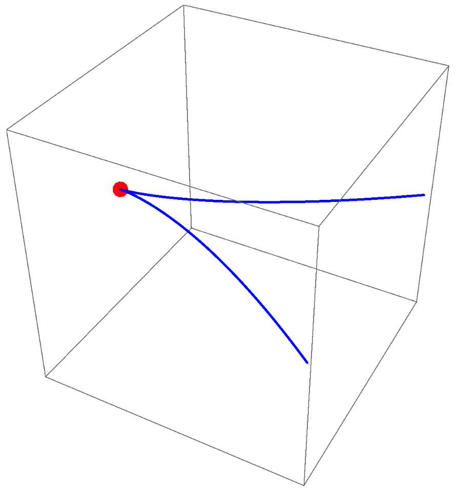
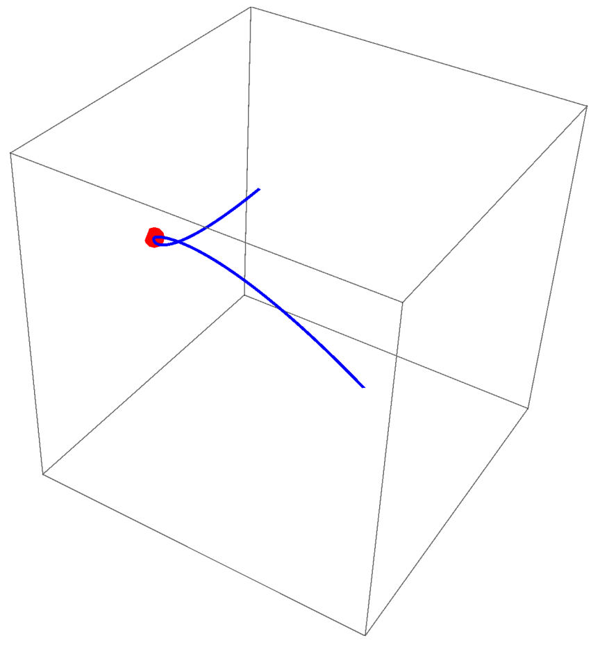
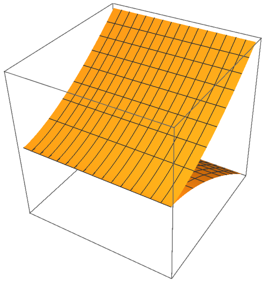
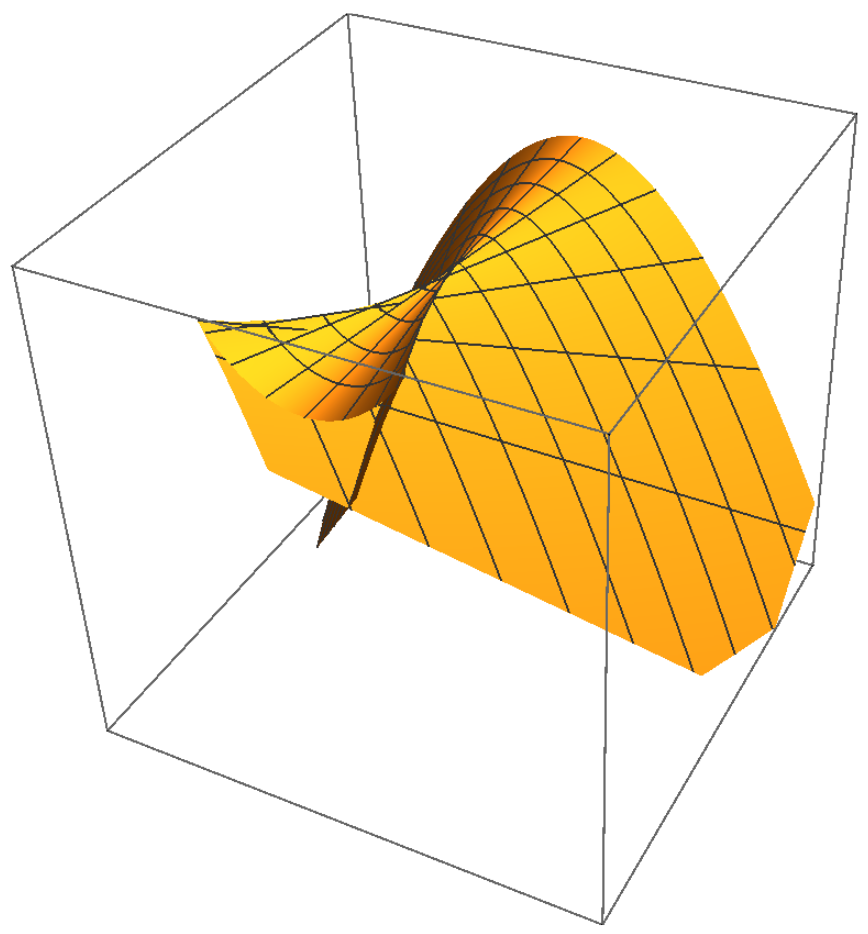
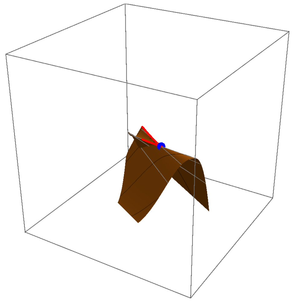
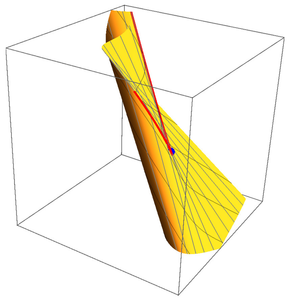
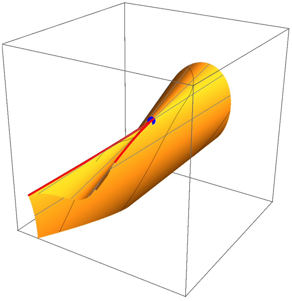
Example 1.

Consider a null Cartan curve $\mathit{\beta }:I\to {\mathbb{R}}_1^4$ equipped with the Cartan frame $\{\mathit{\lambda },\mathit{\xi },{\mathit{w}}_1,{\mathit{w}}_2\}$. The parametric representation of $\mathit{\beta }$ is given by

$$\begin{array}{c}\hfill \mathit{\beta }\left(t\right)=\left(\frac{2}{3}{(3-t)}^{\frac{3}{2}},\frac{2}{3}{(2-t)}^{\frac{3}{2}},cos\left(t\right),sin\left(t\right)\right),\end{array}$$

where I denotes the open interval $(-2,2)$ in the real space $\mathbb{R}$.

Thus, $a\left(t\right)=\frac{5-2t}{2\sqrt{t^2-5t+6}}$, and then, we have

$$\begin{array}{cc}\hfill \mathit{\xi }\left(t\right)=& \frac{2\sqrt{t^2-5t+6}}{5-2t}\left(-\sqrt{3-t},-\sqrt{2-t},-sin\left(t\right),cos\left(t\right)\right).\hfill \end{array}$$

Further, we obtain ${\mathit{w}}_1\left(t\right)=\left(w_{11}\left(t\right),w_{12}\left(t\right),w_{13}\left(t\right),w_{14}\left(t\right)\right)$, where

$$\begin{array}{cc}\hfill w_{11}\left(t\right)=& \frac{-2t^3+15t^2-38t+33}{{(5-2t)}^2\sqrt{3-t}\sqrt{t^2-5t+6}},\hfill \\ \hfill w_{12}\left(t\right)=& \frac{-2t^3+15t^2-38t+32}{{(5-2t)}^2\sqrt{2-t}\sqrt{t^2-5t+6}},\hfill \\ \hfill w_{13}\left(t\right)=& \frac{\left(4t^3-30t^2+74t-60\right)cos\left(t\right)+sin\left(t\right)}{{(5-2t)}^2\sqrt{t^2-5t+6}},\hfill \\ \hfill w_{14}\left(t\right)=& \frac{2\left(2t^3-15t^2+37t-30\right)sin\left(t\right)-cos\left(t\right)}{{(5-2t)}^2\sqrt{t^2-5t+6}},\hfill \end{array}$$

so we calculate

$$\begin{array}{c}\hfill {\kappa }_1\left(t\right)=\frac{16t^6-240t^5+1488t^4-4880t^3+8955t^2-8775t+3621}{8{(5-2t)}^2{(t-3)}^2{(t-2)}^2},\end{array}$$

Hence, let $\mathit{\lambda }\left(t\right)=\left({\lambda }_1\left(t\right),{\lambda }_2\left(t\right),{\lambda }_3\left(t\right),{\lambda }_4\left(t\right)\right)$, where

$$\begin{array}{cc}\hfill {\lambda }_1\left(t\right)=& \frac{8t^5-100t^4+490t^3-1179t^2+1401t-663}{4{(5-2t)}^2\sqrt{3-t}(t-2)\sqrt{t^2-5t+6}},\hfill \\ \hfill {\lambda }_2\left(t\right)=& \frac{8t^5-100t^4+490t^3-1171t^2+1361t-617}{4{(5-2t)}^2\sqrt{2-t}(t-3)\sqrt{t^2-5t+6}},\hfill \\ \hfill {\lambda }_3\left(t\right)=& \frac{\left(8t^5-100t^4+498t^3-1235t^2+1523t-745\right)sin\left(t\right)-8\left(t^2-5t+6\right)cos\left(t\right)}{4{(5-2t)}^2(t-3)(t-2)\sqrt{t^2-5t+6}},\hfill \\ \hfill {\lambda }_4\left(t\right)=& -\frac{8\left(t^2-5t+6\right)sin\left(t\right)+\left(8t^5-100t^4+498t^3-1235t^2+1523t-745\right)cos\left(t\right)}{4{(5-2t)}^2(t-3)(t-2)\sqrt{t^2-5t+6}}.\hfill \end{array}$$

Moreover, ${\mathit{w}}_2\left(t\right)=\left(w_{21}\left(t\right),w_{22}\left(t\right),w_{23}\left(t\right),w_{24}\left(t\right)\right)$ is expressed by

$$\begin{array}{cc}\hfill w_{21}\left(t\right)=& \frac{2\sqrt{2-t}{(t-3)}^2(2t-3)}{{(5-2t)}^2\sqrt{t^2-5t+6}},\hfill \\ \hfill w_{22}\left(t\right)=& \frac{2\sqrt{3-t}{(t-2)}^2(2t-7)}{{(5-2t)}^2\sqrt{t^2-5t+6}},\hfill \\ \hfill w_{23}\left(t\right)=& \frac{\sqrt{2-t}\sqrt{3-t}(2sin\left(t\right)+(2t-5)cos\left(t\right))}{{(5-2t)}^2\sqrt{t^2-5t+6}},\hfill \\ \hfill w_{24}\left(t\right)=& \frac{\sqrt{2-t}\sqrt{3-t}((2t-5)sin\left(t\right)-2cos\left(t\right))}{{(5-2t)}^2\sqrt{t^2-5t+6}}.\hfill \end{array}$$

Therefore, we get

$$\begin{array}{c}\hfill {\kappa }_2\left(t\right)=\frac{4t^2-20t+33}{2{(5-2t)}^2\sqrt{2-t}\sqrt{3-t}}.\end{array}$$

Therefore, the lightlike hypersurface $L{H}_{\mathit{\beta }}$ is defined by the equation

$$\begin{array}{cc}\hfill L{H}_{\mathit{\beta }}(t,\eta ,\mu )& =\left(x_1(t,\eta ,\mu ),\dots ,x_4(t,\eta ,\mu )\right).\hfill \end{array}$$

(2)

(components in Appendix A.1)

The lightlike surface $L{S}_{\mathit{\beta }}$ is defined as follows:

$$\begin{array}{cc}\hfill L{S}_{\mathit{\beta }}(t,\mu )& =\left(y_1(t,\mu ),\dots ,y_4(t,\mu )\right),\hfill \end{array}$$

where

$$\begin{array}{c}\hfill y_1(t,\mu )=x_1(t,{\eta }_0,\mu ),y_2(t,\mu )=x_2(t,{\eta }_0,\mu ),\end{array}$$

$$\begin{array}{c}\hfill y_3(t,\mu )=x_3(t,{\eta }_0,\mu ),y_4(t,\mu )=x_4(t,{\eta }_0,\mu ),\end{array}$$

(expression of ${\eta }_0$, see Appendix A.2)

The curve $L{C}_{\mathit{\beta }}$ is expressed as

$$L{C}_{\mathit{\beta }}\left(t\right)=\left(\frac{z_{11}\left(t\right)}{z_{12}\left(t\right)},\frac{z_{21}\left(t\right)}{z_{22}\left(t\right)},\frac{z_{31}\left(t\right)}{z_{32}\left(t\right)},\frac{z_{41}\left(t\right)}{z_{42}\left(t\right)}\right),$$

(components in Appendix A.3)

We calculate the geometric invariant $\sigma \left(t\right)=\frac{{\sigma }_1\left(t\right)}{{\sigma }_2\left(t\right)}$, (expressions of ${\sigma }_1,{\sigma }_2$; see Appendix A.4).

We verify that the geometric invariant $\sigma \left(t\right)$ has a unique real root $t_0=0.34290545$ within $I=(-2,2)$, with ${\sigma }^{\prime }\left(t_0\right)=-1.7005\ne 0$. By Theorem 1, this implies

• The hypersurface $L{H}_{\mathit{\beta }}$ is locally diffeomorphic to $SW\times \mathbb{R}$ when $t\ne t_0$.
• The surface $L{S}_{\mathit{\beta }}$ is locally diffeomorphic to $C(2,3,4)\times \mathbb{R}$ at $(t,\mu )$, where $\mu ={\mu }_1/{\mu }_2$ (see Appendix A.5 for ${\mu }_1,{\mu }_2$).

At the critical point $t_0=0.34290545$ where $\sigma \left(t_0\right)=0$ and ${\sigma }^{\prime }\left(t_0\right)\ne 0$, Remark 2 establishes

• $L{H}_{\mathit{\beta }}{\sim }_{\mathrm{diff}}BF$
• $L{S}_{\mathit{\beta }}{\sim }_{\mathrm{diff}}C\left(BF\right)$
• $L{C}_{\mathit{\beta }}{\sim }_{\mathrm{diff}}(2,3,4,5)$-cusp at $L{C}_{\mathit{\beta }}\left(t_0\right)=(2.24133,-0.0468908,-0.429587,0.286791)$

While full 4D visualization is impractical, Figure 8, Figure 9, Figure 10 and Figure 11 show 3D projections of $L{H}_{\mathit{\beta }}(t,\eta ,0)$ and $\mu =0$ intersections. Figure 12, Figure 13, Figure 14 and Figure 15 demonstrate that $L{C}_{\mathit{\beta }}$’s projections correspond to critical value sets of $L{S}_{\mathit{\beta }}$, consistent with Remark 2.

Figure 8. $x_1{x}_2{x}_3$-subspace projection of $L{H}_{\mathit{\beta }}$.

Figure 9. $x_1{x}_2{x}_4$-subspace projection of $L{H}_{\mathit{\beta }}$.

Figure 10. $x_1{x}_3{x}_4$-subspace projection of $L{H}_{\mathit{\beta }}$.

Figure 11. $x_2{x}_3{x}_4$-subspace projection of $L{H}_{\mathit{\beta }}$.

Figure 12. $x_1{x}_2{x}_3$-subspace projection of $L{S}_{\mathit{\beta }}$.

Figure 13. $x_1{x}_2{x}_4$-subspace projection of $L{H}_{\mathit{\beta }}$.

Figure 14. $x_1{x}_3{x}_4$-subspace projection of $L{H}_{\mathit{\beta }}$.

Figure 15. $x_2{x}_3{x}_4$-subspace projection of $L{H}_{\mathit{\beta }}$.

Remark 5.

The critical value set of $L{H}_{\mathit{\beta }}(t,\mu ,\eta )$ is divided into three distinct parts (see Figure 12, Figure 13, Figure 14 and Figure 15):

(1)

The gold region represents points $(t,\mu ,\eta )$ where $\mu \ne \frac{{\mu }_1}{{\mu }_2}$ and $\eta ={\eta }_0$.

(2)

The red region represents points $(t,\mu ,\eta )$ where $t\ne 0.34290545$, $\mu =\frac{{\mu }_1}{{\mu }_2}$, and $\eta ={\eta }_0$.

(3)

The blue region represents the point $(t,\mu ,\eta )$ where $t=0.34290545$, $\mu =\frac{{\mu }_1}{{\mu }_2}$, and $\eta ={\eta }_0$.

6. Concluding Remarks

In this study, we have systematically investigated the singularities of lightlike hypersurfaces generated by null Cartan curves in Minkowski spacetime. By leveraging techniques from singularity theory and differential geometry, we established a framework for analyzing singular behavior and introduced a geometric invariant $\sigma \left(t\right)$ governing their stratification. Our results deepen the understanding of lightlike hypersurfaces’ geometric properties and their hierarchical singularity structures.

The exploration of lightlike hypersurfaces along null Cartan curves revealed a hierarchy of singularities, including caustics and higher-order degeneracies. We demonstrated that the singularities of $L{H}_{\mathit{\beta }}$, $L{S}_{\mathit{\beta }}$, and $L{C}_{\mathit{\beta }}$ are interconnected, with each level exhibiting progressive degeneracy. This hierarchical structure provides insights into the global geometry of degenerate submanifolds, particularly in contexts where metric degeneracy drives singularity formation.

A key contribution is the application of unfolding theory to classify singularities. By defining a four-parameter unfolding and proving its $\mathcal{R}$-versality, we rigorously classified singularities into types such as $C(2,3)\times {\mathbb{R}}^2$, $SW\times \mathbb{R}$, and $(2,3,4,5)$-cusp. Explicit examples validate these classifications, underscoring the framework’s utility in geometric analysis.

While this study focused on hypersurfaces generated by regular null Cartan curves, future work could extend to singular null Cartan curves. Such curves, potentially exhibiting singular points, may generate hypersurfaces with novel singularity types, for instance, higher-order caustics or degenerate structures not observed in regular cases. This extension would enrich the classification theory of lightlike submanifolds.

Furthermore, generalizing our framework to pseudo-Riemannian manifolds with curvature presents a significant challenge. The interplay between metric degeneracy and spacetime curvature could yield new singularity phenomena, necessitating adaptations of our algebraic and geometric methods. Such extensions would require addressing non-flat geometry’s analytic complexities while preserving the core classification principles established here.

Beyond theoretical implications, our methods may find applications in analyzing geometric structures across pseudo-Riemannian settings. The hierarchical singularity model could inform studies of degenerate foliations, singular energy concentrations, or stratified geometries in higher dimensions. Additionally, the techniques developed here might adapt to other lightlike submanifold classes, such as those in spacetimes with additional symmetry or geometric constraints.

In conclusion, this work establishes foundational connections between lightlike hypersurfaces, singularity theory, and contact geometry in Minkowski spacetime. By bridging differential geometry and singularity analysis, it opens avenues for exploring degenerate structures in broader mathematical contexts. We anticipate that these results will stimulate further research into the intricate geometry of lightlike submanifolds and their stratified singularities.

Appendix A.1. Lightlike Hypersurface Components

The coordinates $x_i(t,\eta ,\mu )$ of $L{H}_{\mathit{\beta }}$: where

$$\begin{array}{cc}\hfill x_1(t,\eta ,\mu )=& \frac{2}{3}{(3-t)}^{3/2}+\frac{\eta \left(8t^5-100t^4+490t^3-1179t^2+1401t-663\right)}{4{(5-2t)}^2\sqrt{3-t}(t-2)\sqrt{t^2-5t+6}}\hfill \\ \hfill & +\frac{4\sqrt{t^2-5t+6}\sqrt{2-t}\left(-2t^3+15t^2-38t+33\right)\left(-\frac{\mu \left(4t^2-20t+33\right)}{{(5-2t)}^2}-2t+5\right)}{16t^6-240t^5+1488t^4-4880t^3+8955t^2-8775t+3621}\hfill \\ \hfill & +\frac{2\mu (2t-3){(3-t)}^{3/2}}{{(5-2t)}^2},\hfill \end{array}$$

$$\begin{array}{cc}\hfill x_2(t,\eta ,\mu )=& \frac{2}{3}{(2-t)}^{3/2}+\frac{\eta \left(8t^5-100t^4+490t^3-1171t^2+1361t-617\right)}{4{(5-2t)}^2\sqrt{2-t}(t-3)\sqrt{t^2-5t+6}}\hfill \\ \hfill & +\frac{4\sqrt{t^2-5t+6}\sqrt{3-t}\left(-2t^3+15t^2-38t+32\right)\left(-\frac{\mu \left(4t^2-20t+33\right)}{{(5-2t)}^2}-2t+5\right)}{16t^6-240t^5+1488t^4-4880t^3+8955t^2-8775t+3621}\hfill \\ \hfill & +\frac{2\mu {(t-2)}^{3/2}(2t-7)}{{(5-2t)}^2},\hfill \end{array}$$

$$\begin{array}{cc}\hfill x_3(t,\eta ,\mu )=& \frac{\eta \left(\left(8t^5-100t^4+498t^3-1235t^2+1523t-745\right)sin\left(t\right)-8\left(t^2-5t+6\right)cos\left(t\right)\right)}{4{(5-2t)}^2(t-3)(t-2)\sqrt{t^2-5t+6}}\hfill \\ \hfill & +\frac{4(t-3)(t-2)\left(-\frac{\mu \left(4t^2-20t+33\right)}{{(5-2t)}^2}-2t+5\right)\left(\left(4t^3-30t^2+74t-60\right)cos\left(t\right)+sin\left(t\right)\right)}{16t^6-240t^5+1488t^4-4880t^3+8955t^2-8775t+3621}\hfill \\ \hfill & +\frac{\mu (2sin(t)+(2t-5)cos(t\left)\right)}{{(5-2t)}^2}+cos\left(t\right),\hfill \end{array}$$

$$\begin{array}{cc}\hfill x_4(t,\eta ,\mu )=& -\frac{\eta \left(8\left(t^2-5t+6\right)sin\left(t\right)+\left(8t^5-100t^4+498t^3-1235t^2+1523t-745\right)cos\left(t\right)\right)}{4{(5-2t)}^2(t-3)(t-2)\sqrt{t^2-5t+6}}\hfill \\ \hfill & +\frac{4(t-3)(t-2)\left(-\frac{\mu \left(4t^2-20t+33\right)}{{(5-2t)}^2}-2t+5\right)\left(2\left(2t^3-15t^2+37t-30\right)sin\left(t\right)-cos\left(t\right)\right)}{16t^6-240t^5+1488t^4-4880t^3+8955t^2-8775t+3621}\hfill \\ \hfill & +\frac{\mu \left(\right(2t-5)sin(t)-2cos(t\left)\right)}{{(5-2t)}^2}+sin\left(t\right).\hfill \end{array}$$

Appendix A.2. The Expression of η 0

$$\begin{array}{cc}\hfill {\eta }_0=& (-\frac{16t^6-240t^5+1272t^4-2720t^3+873t^2+4635t-4704}{2{(t^2-5t+6)}^{3/2}}\hfill \\ \hfill & -\frac{16t^6-240t^5+1488t^4-4880t^3+8955t^2-8775t+3621}{4{(t^2-5t+6)}^{3/2}}\hfill \\ \hfill & +(-\frac{4t^2-20t+33}{2{(2t-5)}^3{(t^2-5t+6)}^{3/2}}\times (16t^6-240t^5+1272t^4-2720t^3+873t^2\hfill \\ \hfill & +4635t-4704)+\frac{(-16t^4+160t^3-696t^2+1480t-1209)}{4{(2t-5)}^3{(t^2-5t+6)}^{3/2}}(16t^6-240t^5\hfill \\ \hfill & +1488t^4-4880t^3+8955t^2-8775t+3621\left)\right)\mu )/((16t^6-240t^5+1488t^4\hfill \\ \hfill & -4880t^3+8955t^2-8775t+3621\left)\right(\frac{1}{64{(5-2t)}^4(t^2-5t+6^4}(16t^6-240t^5\hfill \\ \hfill & +1488t^4-4880t^3+8955t^2{-8775t+3621)}^2+\frac{{(4t^2-20t+33)}^2}{4{(5-2t)}^4(t^2-5t+6)}\left)\right).\hfill \end{array}$$

Appendix A.3. Spacelike Critical Curve Components

The coordinates $z_i\left(t\right)=\frac{z_{i1}\left(t\right)}{z_{i2}\left(t\right)}$ of $L{C}_{\mathit{\beta }}$: where

$$\begin{array}{cc}\hfill z_{11}\left(t\right)=& 8{(3-t)}^{5/2}(8192t^{21}-413696t^{20}+9895936t^{19}-149069824t^{18}+1585539584t^{17}\hfill \\ \hfill & -12651908352t^{16}+78534498816t^{15}-387908872704t^{14}+1545891750240t^{13}\hfill \\ \hfill & -5006570697712t^{12}+13193545876864t^{11}-28141449044480t^{10}+47889219934238t^9\hfill \\ \hfill & -63039105928735t^8+59726954767710t^7-31837092002076t^6-7985877345978t^5\hfill \\ \hfill & +35341769165517t^4-36786629934792t^3+21494853768564t^2-7124973744960t\hfill \\ \hfill & +1049941063377),\hfill \end{array}$$

$$\begin{array}{cc}\hfill z_{12}\left(t\right)=& 3(16384t^{22}-901120t^{21}+23736320t^{20}-398336000t^{19}+4779811840t^{18}\hfill \\ \hfill & -43635532800t^{17}+314843972352t^{16}-1841228974080t^{15}+8878508714688t^{14}\hfill \\ \hfill & -35717296854080t^{13}+120787321038608t^{12}-344821503982240t^{11}\hfill \\ \hfill & +831968373735532t^{10}-1693534936358300t^9+2894429815286841t^8\hfill \\ \hfill & -4119307919891820t^7+4821298311148428t^6-4557680182229670t^5\hfill \\ \hfill & +3389956568216271t^4-1907403448920210t^3+761968194267834t^2\hfill \\ \hfill & -192235414177170t+22978966883823,\hfill \end{array}$$

$$\begin{array}{cc}\hfill z_{21}\left(t\right)=& 8{(2-t)}^{5/2}(8192t^{21}-446464t^{20}+11534336t^{19}-187908096t^{18}\hfill \\ \hfill & +2165901824t^{17}-18783327488t^{16}+127220128256t^{15}-689414122496t^{14}\hfill \\ \hfill & +3037307012960t^{13}-10992019026288t^{12}+32876142550144t^{11}\hfill \\ \hfill & -81464530998240t^{10}+167091315418238t^9-282455510241975t^8\hfill \\ \hfill & +390275807232510t^7-435047251652274t^6+383671652236992t^5\hfill \\ \hfill & -260076523775067t^4+129718864097298t^3-44391618920484t^2\hfill \\ \hfill & +9190533358530t-855882111177).\hfill \end{array}$$

$$\begin{array}{cc}\hfill z_{22}\left(t\right)=& 3(16384t^{22}-901120t^{21}+23736320t^{20}-398336000t^{19}+4779811840t^{18}\hfill \\ \hfill & -43635532800t^{17}+314843972352t^{16}-1841228974080t^{15}+8878508714688t^{14}\hfill \\ \hfill & -35717296854080t^{13}+120787321038608t^{12}-344821503982240t^{11}\hfill \\ \hfill & +831968373735532t^{10}-1693534936358300t^9+2894429815286841t^8\hfill \\ \hfill & -4119307919891820t^7+4821298311148428t^6-4557680182229670t^5\hfill \\ \hfill & +3389956568216271t^4-1907403448920210t^3+761968194267834t^2\hfill \\ \hfill & -192235414177170t+22978966883823)\hfill \end{array}$$

$$\begin{array}{cc}\hfill z_{31}\left(t\right)& =2\left(\right(8192t^{21}-430080t^{20}+10838016t^{19}-174325760t^{18}+2006981120t^{17}\hfill \\ \hfill & -17575225600t^{16}+121425492992t^{15}-677510387200t^{14}+3099815318880t^{13}\hfill \\ \hfill & -11743333383600t^{12}+37044917181472t^{11}-97532408400480t^{10}\hfill \\ \hfill & +214167820946958t^9-390791714591555t^8+588403768560908t^7-722968220401140t^6\hfill \\ \hfill & +712949223584184t^5-550498829290425t^4+320453671834386t^3-132170582322270t^2\hfill \\ \hfill & +34402571621748t-4244885728245)sin\left(t\right)-4(4096t^{20}-204800t^{19}+4956160t^{18}\hfill \\ \hfill & -77107200t^{17}+862990592t^{16}-7363143680t^{15}+49522955264t^{14}-267960074240t^{13}\hfill \\ \hfill & +1181021233712t^{12}-4270611283360t^{11}+12711251200704t^{10}-31141333447600t^9\hfill \\ \hfill & +62594316359483t^8-102533203149660t^7+135383407823862t^6-141713414212680t^5\hfill \\ \hfill & +114700443528987t^4-69081662638620t^3+29071542765564t^2-7602714301320t\hfill \\ \hfill & +925878403413)cos(t\left)\right),\hfill \end{array}$$

$$\begin{array}{cc}\hfill z_{32}\left(t\right)=& 16384t^{22}-901120t^{21}+23736320t^{20}-398336000t^{19}+4779811840t^{18}\hfill \\ \hfill & -43635532800t^{17}+314843972352t^{16}-1841228974080t^{15}+8878508714688t^{14}\hfill \\ \hfill & -35717296854080t^{13}+120787321038608t^{12}-344821503982240t^{11}\hfill \\ \hfill & +831968373735532t^{10}-1693534936358300t^9+2894429815286841t^8\hfill \\ \hfill & -4119307919891820t^7+4821298311148428t^6-4557680182229670t^5\hfill \\ \hfill & +3389956568216271t^4-1907403448920210t^3+761968194267834t^2\hfill \\ \hfill & -192235414177170t+22978966883823,\hfill \end{array}$$

$$\begin{array}{cc}\hfill z_{41}\left(t\right)=& -2\left(4\right(4096t^{20}-204800t^{19}+4956160t^{18}-77107200t^{17}+862990592t^{16}\hfill \\ \hfill & -7363143680t^{15}+49522955264t^{14}-267960074240t^{13}+1181021233712t^{12}\hfill \\ \hfill & -4270611283360t^{11}+12711251200704t^{10}-31141333447600t^9\hfill \\ \hfill & +62594316359483t^8-102533203149660t^7+135383407823862t^6\hfill \\ \hfill & -141713414212680t^5+114700443528987t^4-69081662638620t^3\hfill \\ \hfill & +29071542765564t^2-7602714301320t+925878403413)sin\left(t\right)\hfill \\ \hfill & +(8192t^{21}-430080t^{20}+10838016t^{19}-174325760t^{18}+2006981120t^{17}\hfill \\ \hfill & -17575225600t^{16}+121425492992t^{15}-677510387200t^{14}+3099815318880t^{13}\hfill \\ \hfill & -11743333383600t^{12}+37044917181472t^{11}-97532408400480t^{10}\hfill \\ \hfill & +214167820946958t^9-390791714591555t^8+588403768560908t^7\hfill \\ \hfill & -722968220401140t^6+712949223584184t^5-550498829290425t^4\hfill \\ \hfill & +320453671834386t^3-132170582322270t^2+34402571621748t\hfill \\ \hfill & -4244885728245)cos(t\left)\right),\hfill \end{array}$$

$$\begin{array}{cc}\hfill z_{42}\left(t\right)=& 16384t^{22}-901120t^{21}+23736320t^{20}-398336000t^{19}+4779811840t^{18}\hfill \\ \hfill & -43635532800t^{17}+314843972352t^{16}-1841228974080t^{15}\hfill \\ \hfill & +8878508714688t^{14}-35717296854080t^{13}+120787321038608t^{12}\hfill \\ \hfill & -344821503982240t^{11}+831968373735532t^{10}-1693534936358300t^9\hfill \\ \hfill & +2894429815286841t^8-4119307919891820t^7+4821298311148428t^6\hfill \\ \hfill & -4557680182229670t^5+3389956568216271t^4-1907403448920210t^3\hfill \\ \hfill & +761968194267834t^2-192235414177170t+22978966883823.\hfill \end{array}$$

Appendix A.4. Expressions of Invariant

$$\begin{array}{cc}\hfill {\sigma }_1\left(t\right)=& 0.5t^{64}-80.t^{63}+6307.25t^{62}-326624.t^{61}+1.24955\times {10}^7{t}^{60}-3.76587\times {10}^8{t}^{59}\hfill \\ \hfill & +9.31103\times {10}^9{t}^{58}-1.94205\times {10}^{11}{t}^{57}+3.48725\times {10}^{12}{t}^{56}-5.47488\times {10}^{13}{t}^{55}\hfill \\ \hfill & +7.60667\times {10}^{14}{t}^{54}-9.44426\times {10}^{15}{t}^{53}+1.05622\times {10}^{17}{t}^{52}-1.07108\times {10}^{18}{t}^{51}\hfill \\ \hfill & +9.90356\times {10}^{18}{t}^{50}-8.38911\times {10}^{19}{t}^{49}+6.5366\times {10}^{20}{t}^{48}-4.70124\times {10}^{21}{t}^{47}\hfill \\ \hfill & +3.13044\times {10}^{22}{t}^{46}-1.93492\times {10}^{23}{t}^{45}+1.11269\times {10}^{24}{t}^{44}-5.96474\times {10}^{24}{t}^{43}\hfill \\ \hfill & +2.98576\times {10}^{25}{t}^{42}-1.39767\times {10}^{26}{t}^{41}+6.12619\times {10}^{26}{t}^{40}-2.51696\times {10}^{27}{t}^{39}\hfill \\ \hfill & +9.70184\times {10}^{27}{t}^{38}-3.51113\times {10}^{28}{t}^{37}+1.19375\times {10}^{29}{t}^{36}-3.8146\times {10}^{29}{t}^{35}\hfill \\ \hfill & +1.14603\times {10}^{30}{t}^{34}-3.23774\times {10}^{30}{t}^{33}+8.60237\times {10}^{30}{t}^{32}-2.14934\times {10}^{31}{t}^{31}\hfill \\ \hfill & +5.04933\times {10}^{31}{t}^{30}-1.11502\times {10}^{32}{t}^{29}+2.31353\times {10}^{32}{t}^{28}-4.50804\times {10}^{32}{t}^{27}\hfill \\ \hfill & +8.24393\times {10}^{32}{t}^{26}-1.41375\times {10}^{33}{t}^{25}+2.27144\times {10}^{33}{t}^{24}-3.41543\times {10}^{33}{t}^{23}\hfill \\ \hfill & +4.80022\times {10}^{33}{t}^{22}-6.29687\times {10}^{33}{t}^{21}+7.69702\times {10}^{33}{t}^{20}-8.75065\times {10}^{33}{t}^{19}\hfill \\ \hfill & +9.23319\times {10}^{33}{t}^{18}-9.01988\times {10}^{33}{t}^{17}+8.13545\times {10}^{33}{t}^{16}-6.75326\times {10}^{33}{t}^{15}\hfill \\ \hfill & +5.14054\times {10}^{33}{t}^{14}-3.57299\times {10}^{33}{t}^{13}+2.25655\times {10}^{33}{t}^{12}-1.28748\times {10}^{33}{t}^{11}\hfill \\ \hfill & +6.5909\times {10}^{32}{t}^{10}-3.00251\times {10}^{32}{t}^9+1.20505\times {10}^{32}{t}^8-4.20819\times {10}^{31}{t}^7\hfill \\ \hfill & +1.25854\times {10}^{31}{t}^6-3.15705\times {10}^{30}{t}^5+6.45608\times {10}^{29}{t}^4-1.03277\times {10}^{29}{t}^3\hfill \\ \hfill & +1.21083\times {10}^{28}{t}^2-9.24005\times {10}^{26}t+3.43801\times {10}^{25},\hfill \end{array}$$

$$\begin{array}{cc}\hfill {\sigma }_2\left(t\right)=& {(t-3.)}^{10}{(t-2.)}^{10}\sqrt{t^2-5t+6}(t^{10}-25t^9+280.75t^8-1865t^7+8123.19t^6\hfill \\ \hfill & -24285.3t^5+50609.2t^4-72849.8t^3+69599.7t^2-40012t+10547\left)\right(t^{30}\hfill \\ \hfill & -75.t^{29}+2723.25t^{28}-63752.5t^{27}+1.08119\times {10}^6{t}^{26}-1.41505\times {10}^7{t}^{25}\hfill \\ \hfill & +1.48674\times {10}^8{t}^{24}-1.28794\times {10}^9{t}^{23}+9.37617\times {10}^9{t}^{22}-5.81723\times {10}^{10}{t}^{21}\hfill \\ \hfill & +3.10843\times {10}^{11}{t}^{20}-1.44194\times {10}^{12}{t}^{19}+5.84123\times {10}^{12}{t}^{18}-2.07527\times {10}^{13}{t}^{17}\hfill \\ \hfill & +6.48489\times {10}^{13}{t}^{16}-1.78522\times {10}^{14}{t}^{15}+4.33144\times {10}^{14}{t}^{14}-9.25574\times {10}^{14}{t}^{13}\hfill \\ \hfill & +1.73863\times {10}^{15}{t}^{12}-2.86184\times {10}^{15}{t}^{11}+4.10906\times {10}^{15}{t}^{10}-5.1144\times {10}^{15}{t}^9\hfill \\ \hfill & +5.4729\times {10}^{15}{t}^8-4.98075\times {10}^{15}{t}^7+3.79993\times {10}^{15}{t}^6-2.38351\times {10}^{15}{t}^5\hfill \\ \hfill & +1.19627\times {10}^{15}{t}^4-4.61603\times {10}^{14}{t}^3+1.28479\times {10}^{14}{t}^2-2.29425\times {10}^{13}t\hfill \\ \hfill & +1.9723\times {10}^{12}{)(2.5-1.t)}^4.\hfill \end{array}$$

Appendix A.5. Expressions of Curvatures Coupling Functions

$$\begin{array}{cc}\hfill {\mu }_1=& -(2t-5)(16384t^{22}-901120t^{21}+23638016t^{20}-393420800t^{19}+4662469632t^{18}\hfill \\ \hfill & -41857213440t^{17}+295661144832t^{16}-1684727777280t^{15}+7877054397120t^{14}\hfill \\ \hfill & -30573467739200t^{13}+99263605245584t^{12}-270782428527520t^{11}\hfill \\ \hfill & +621617248349932t^{10}-1199479736358300t^9+1937616017756049t^8\hfill \\ \hfill & -2601016378075980t^7+2868296467564476t^6-2554517017356390t^5\hfill \\ \hfill & +1791739295842599t^4-952607770853490t^3+360729531699354t^2\hfill \\ \hfill & -86663131618770t+9927643179159),\hfill \end{array}$$

$$\begin{array}{cc}\hfill {\mu }_2=& 16384t^{22}-901120t^{21}+23736320t^{20}-398336000t^{19}+4779811840t^{18}\hfill \\ \hfill & -43635532800t^{17}+314843972352t^{16}-1841228974080t^{15}+8878508714688t^{14}\hfill \\ \hfill & -35717296854080t^{13}+120787321038608t^{12}-344821503982240t^{11}\hfill \\ \hfill & +831968373735532t^{10}-1693534936358300t^9+2894429815286841t^8\hfill \\ \hfill & -4119307919891820t^7+4821298311148428t^6-4557680182229670t^5\hfill \\ \hfill & +3389956568216271t^4-1907403448920210t^3+761968194267834t^2\hfill \\ \hfill & -192235414177170t+22978966883823.\hfill \end{array}$$