A Novel Method to Identify Important Edges in a Directed Network

Abstract

Identifying the key components in complex systems is crucial for ensuring the functionality and integrity of the system. For directed networks, both nodes and edges are critical components, but little attention has been drawn to the important edges. In this paper, a novel method, Cooperation–Competition Centrality (Co-Com Centrality), has been proposed to quantify the edge importance in a directed network. This method utilizes cooperation and competition relationships to integrate the local and global information about the network. We compare the performance of Co-Com Centrality with five typical methods in nine networks; the experiments show that Co-Com Centrality can accurately identify edges which are crucial for maintaining global network efficiency and network stability, while also accurately assessing the edge importance.

1. Introduction

A river network area is densely populated and faces a high risk of water-related disasters [1,2,3]. Protecting the normal functioning of the river network system is crucial for the socio-economic stability of a region [4,5]. The river network is a typical complex system consisting of numerous interwoven river segments; the lake is the node, and the river is the edge. Considering the interaction between rivers, how to analyze the importance of each lake and river from the perspective of the entire river network is an urgent problem to be solved. In recent years, with the development of network science, complex network theory has provided us with an effective tool for river network analysis.

Complex network theory has developed many methods for assessing node importance. Degree Centrality [6], H-index [7], k-shell [8], and Semi-local Centrality [9] are based on the degree of a node. Closeness Centrality [10], Betweenness Centrality [11], and Eccentricity Centrality [12] are based on paths in networks. Eigenvector Centrality, Katz Centrality [13], and PageRank Centrality [14] are based on the neighbors of a node. Current-flow Centrality [15], Entanglement Centrality [16], and Random-walk Centrality [17] are based on the function of nodes in dynamical processes. Recently, Engsig et al. [18] proposed DomiRank Centrality based on the competitive relationships between nodes; this method can efficiently identify those nodes that are in a dominant position.

The number of studies evaluating edge importance is also rapidly increasing. There are numerous methods to identify edge importance based on the relevant concepts of neighborhoods [19,20,21,22,23,24,25,26]; they have achieved good results in their respective fields, but they cannot be directly extended to directed networks. Considering that the flow of a river has a certain direction (for example, the Yangtze River flows from west to east), we need a method to analyze the edge importance for the directed network. Some path-based methods [27,28,29,30] can be applied to directed networks, but they often face high computational costs. Restrepo et al. [31] measure edge importance according to the change in the largest eigenvalue of the adjacency matrix of the directed networks by deleting an edge. Kim et al. [32] identify edge importance in the directed networks based on PageRank, but the method in [32] cannot be applied to all kinds of directed networks because the definition of direction does not have a universal meaning in all kinds of directed networks. Lehnertz et al. [33] directly extend the definition of Closeness Centrality and Eigenvector Centrality to edges, and they can be applied to directed networks.

In this paper, we propose a new centrality: Cooperation–Competition Centrality (Co-Com Centrality). In simple terms, it reveals the edge importance in the directed networks, which is determined by the topological information of the edges and the intensity of the cooperation and competition. This centrality can be adjusted by cooperation parameter $\alpha$ and competition parameter $\beta$. The time complexity of Co-Com Centrality is $O\left(m^2/n+m\right)$, where n is the number of nodes and m is the number of edges.

Thus, the main contributions of this work are summarized as follows.

1.

We propose a new method for identifying the edge importance of directed networks. Compared with the traditional methods, Co-Com Centrality can more accurately identify the edges that maintain global network efficiency and network stability.

2.

We defined a local-based edge importance by utilizing the out-degree and in-degree of nodes. Moreover, we introduce the concepts of competition and cooperation for directed edges and use a differential equation to aggregate the global information of a network. Benefiting from this, Co-Com Centrality can distinguish more subtle differences between edges.

The structure design of this article is as follows: Section 2 gives a series of typical methods for comparison, including Edge Betweenness Centrality (EBC), Edge Closeness Centrality (ECC), Edge Eigenvector Centrality (EEC), LinkRank (LR), and Edge Dynamical Importance (EDY). Section 3 introduces the new method, Co-Com centrality, in detail. Section 4 shows network datasets, experiment results and the discussion on the comparison between Co-Com Centrality and the five typical methods. Section 5 concludes this paper and discusses future research directions.

2. Related Works

2.1. Edge Betweenness Centrality

Edge Betweenness Centrality (EBC) [28] measures the edge importance by the number of its shortest paths; it is a method suitable for undirected and directed networks. It is defined as

$$EBC\left(k\right)=\sum _{s\ne t}{\displaystyle \frac{{\sigma }_{st}\left(k\right)}{{\sigma }_{st}}},$$

(1)

where ${\sigma }_{st}$ is the number of shortest paths from node s to node t, and ${\sigma }_{st}\left(k\right)$ is the number of shortest paths from node t to node s that pass through edge k.

2.2. Edge Closeness Centrality

Edge Closeness Centrality (ECC) [33] measures the edge importance by the sum of the length from its shortest path to other edges; it is a method suitable for undirected and directed networks. It is defined as

$$ECC\left(k\right)={\displaystyle \frac{m-1}{{\sum }_l{d}_{lk}}},$$

(2)

with $\{l,k\}\in \mathcal{E}$ and $\mathcal{E}$ denotes the edge set of network, where m is the number of edges and $d_{lk}$ denotes the minimum number of edges required to pass from edge l to edge k (define $d_{ij}$ = 1, if edges i and j connect to the same node).

2.3. Edge Eigenvector Centrality

Edge Eigenvector Centrality (EEC) [33] measures the edge importance by the importance of its neighbors; it is a method suitable for undirected and directed networks. It is defined as

$$EEC\left(k\right)={\displaystyle \frac{1}{{\lambda }_{\max }}}\sum _l{M}_{kl}EEC\left(l\right),$$

(3)

with $\{k,l\}\in \mathcal{E}$, where ${\lambda }_{\max }$ is the maximal eigenvalue of M, and M denotes the edge adjacency matrix, with $M_{kl}=1$ if edge k directly connects to edge l and 0 otherwise.

2.4. LinkRank

LinkRank (LR) [32] measures the edge importance by the probability of a random walker following some edge from node $n_i$ to $n_j$ in the stationary state; it is a method for directed networks. It is defined as

$$LR\left(k\right)={\pi }_i{G}_{ij},$$

(4)

where i is the source of edge k, j is the target of edge k, ${\pi }_i$ is the ith element of PageRank vector $\pi$, and $G_{ij}$ is the element of Google Matrix $\mathit{G}$ [14].

2.5. Edge Dynamical Importance

Edge Dynamical Importance (EDY) [31] measures edge importance based on the impact of deleting an edge on the largest eigenvalue of the adjacency matrix of a directed network; it is a method for directed networks. It is defined as

$$EDY\left(k\right)=-{\displaystyle \frac{\Delta {\lambda }_{ij}}{\lambda }},$$

(5)

where i is the source of edge k, j is the target of edge k, $\lambda$ is the largest eigenvalue of the adjacency matrix, and $-\Delta {\lambda }_{ij}$ is the amount by which the $\lambda$ decreases after removing k. Equation (5) can be approximated by

$$E\widehat{D}Y\left(k\right)={\displaystyle \frac{A_{ij}{v}_i{u}_j}{\lambda V^{T}U}},$$

(6)

where A is the adjacency matrix of the network, U and V are the right and left eigenvectors of $\lambda$, and $v_i$ and $u_j$ are the ith and jth elements of eigenvectors.

3. Proposed Method

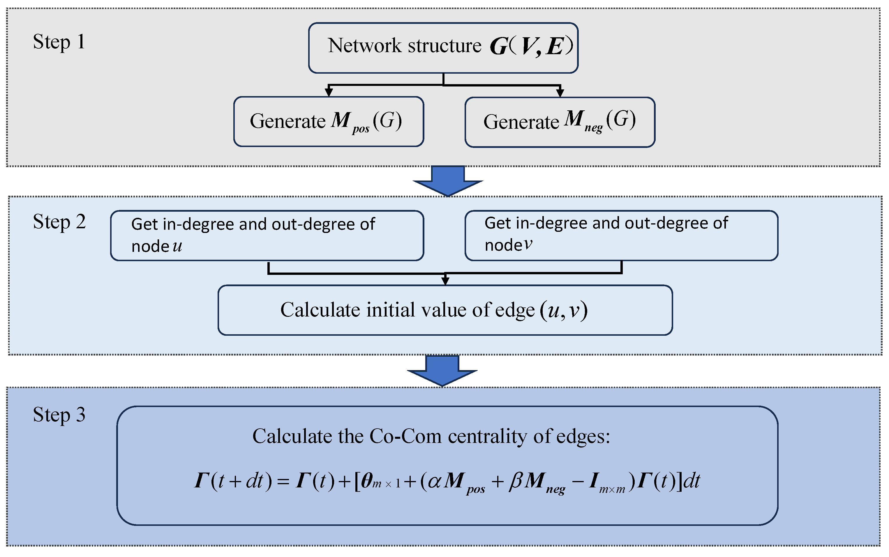
3.1. Definition of Co-Com Centrality

A classic idea [28] holds that, in network transportation, the higher the frequency with which an edge serves as a path that must be traversed from one region to another, the greater its importance. Guided by this idea, we propose a method to measure the importance of edges in a directed graph by utilizing local information, that is, to define the importance of an edge by using all the edges that have the same nodes with this edge. For a directed edge $(u,v)$, u is the source and v is the target; the more edges that point to u and the more edges that originate from v, the more important the edge $(u,v)$ is. If there are other edges originating from u or other edges pointing to v, the irreplaceability of $(u,v)$ will reduce, and the importance of $(u,v)$ will also reduce. So the importance of edge $(u,v)$ is defined as

$${\mathit{V}}_{(u,v)}={\displaystyle \frac{u_{in}}{u_{out}}}+{\displaystyle \frac{v_{out}}{v_{in}}},$$

(7)

where u is the source of a directed edge, and v is the target of the directed edge. $u_{in}$ is the in-degree of u, $u_{out}$ is the out-degree of u, $v_{in}$ is the in-degree of v, and $v_{out}$ is the out-degree of v. Consider that $u_{out}$ and $v_{in}$ are at least one because there is an edge from u to v. We do not use multiplication because for those edges where the in-degree of u is 0 or the out-degree of v is 0, using multiplication will make their importance become 0, which will reduce the discriminability of edge importance. For weighted networks, we only need to change Equation (7) to Equation (8),

$$V_{(u,v)}=w_{(u,v)}\left[{\displaystyle \frac{{\sum }_{i\in p}{w}_{(i,u)}}{{\sum }_{i\in q}{w}_{(u,i)}}}+{\displaystyle \frac{{\sum }_{i\in r}{w}_{(v,i)}}{{\sum }_{i\in s}{w}_{(i,v)}}}\right],$$

(8)

where p is the set of the predecessors of node u, q is the set of the successors of node u, r is the set of the successors of node v, and s is the set of the predecessors of node v. $w_{(u,v)}$ is the weight of edge ($u,v$). The experiments in Section 4 show that the edge importance defined by Equation (7) can already identify important edges quite well. However, the edge importance defined solely by local information poses problems in certain situations. 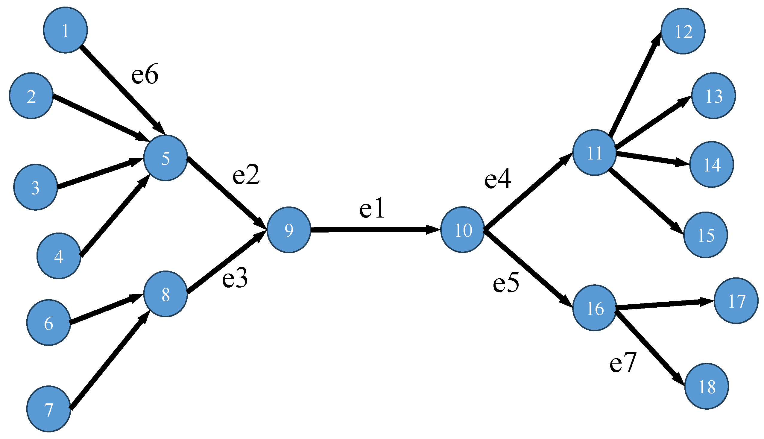See Figure 1; from the perspective of maintaining the network structure, it is obvious that $e1$ is the most important edge but, according to Equation (7), the importance value of $e2$ is $4.5$ and the importance value of $e1$ is 4. This is because Equation (7) only takes local information into account. We need a method to consider global information, the whole network.

Our proposed method is inspired by some simple physical phenomena: assume that there is a directed river network. (i) If the flow of a river increases, the flow of its downstream rivers will increase accordingly; ($ii$) if the flow of a river increases, we can speculate that the flow of its upstream rivers has increased; ($iii$) assume river A and river B have the same upstream, then the flow of either A or B will not increase indefinitely; when the flow of A becomes too high, more water from the upstream will flow into B; then, the flow of A will relatively decrease; ($iv$) assume river C and river D have the same downstream, then the flow of either C or D will not decrease indefinitely; when the flow of C becomes too low, more water from D will flow into downstream; the flow of C will relatively increase.

We map this relationship in a river network into a directed network and use Figure 1 for illustration. Regard the flow of river as a kind of edge importance; then, for the directed network, the importance of each edge will satisfy the following relation: (i) the importance of edge ($u,v$) is positively correlated with the importance of the predecessor edges of node u (the importance of $e2$ is positively correlated with $e6$); ($ii$) the importance of edge ($u,v$) is positively correlated with the importance of the successor edges of node v (the importance of $e2$ is positively correlated with $e1$); ($iii$) the importance of edge ($u,v$) is negatively correlated with the importance of the successor edges of node u (the importance of $e4$ is negatively correlated with the importance of $e5$); ($iv$) the importance of edge ($u,v$) is negatively correlated with the importance of the predecessor edges of node v (the importance of $e2$ is negatively correlated with $e3$).

Regarding positive correlation as cooperation and negative correlation as competition, we propose Co-Com Centrality (Cooperation–Competition Centrality); cooperation matrix $M_{pos}$ and competition matrix $M_{neg}$ are defined to describe cooperation and competition. The diagonal elements of $M_{pos}$ are 0, the other elements are 0 or 1; if $M_{pos(i,j)}$ is 1, it indicates that the ith edge and the jth edge have a cooperative relationship. The diagonal elements of $M_{neg}$ are also 0, but the difference is that the elements are represented by 0 or $-1$; if $M_{neg(i,j)}$ is $-1$, it indicates that the ith edge and the jth edge have a competition relationship. 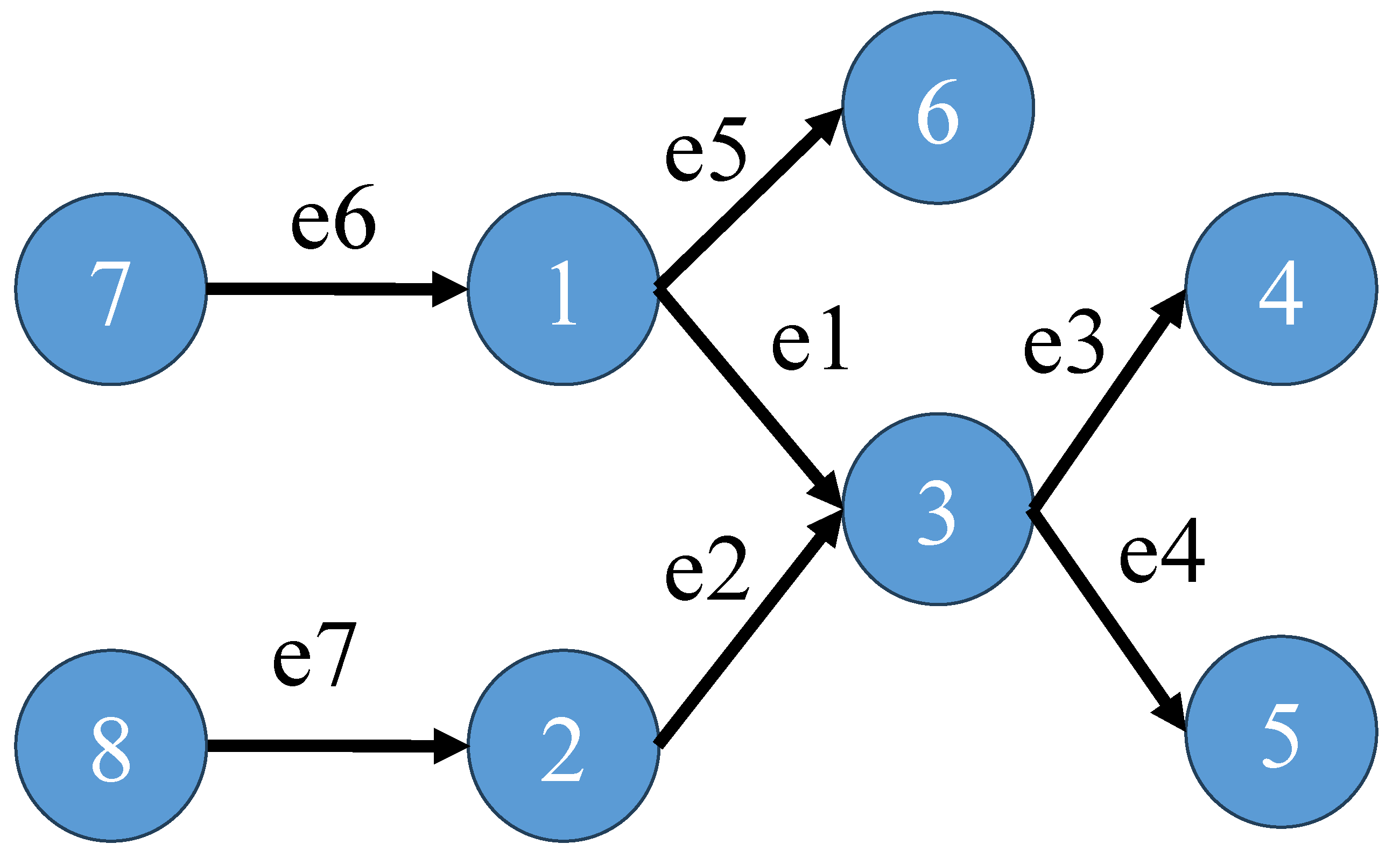Figure 2 gives a simple example to demonstrate the cooperation matrix and the competition matrix; in this network, $e1$ competes with $e2$, $e5$ and cooperates with $e3$, $e4$, $e6$; $M_{pos}$ and $M_{neg}$ are shown as Equation (9).

$$M_{pos}=\begin{array}{cc}\hfill \begin{array}{ccccccc}e1& e2& e3\hfill & e4& e5& e6& e7\end{array}\hfill & \hfill \hspace{1em}\\ \left(\begin{array}{ccccccc}\hfill \begin{array}{c}\hfill 0\end{array}& 0& 1\hfill & 1& 0& 1& 0\\ \hfill 0& 0& 1\hfill & 1& 0& 0& 1\\ \hfill 1& 1& 0\hfill & 0& 0& 0& 0\\ \hfill 1& 1& 0\hfill & 0& 0& 0& 0\\ \hfill 0& 0& 0\hfill & 0& 0& 1& 0\\ \hfill 1& 0& 0\hfill & 0& 1& 0& 0\\ \hfill 0& 1& 0\hfill & 0& 0& 0& 0\end{array}\right)& \begin{array}{c}e1\\ e2\\ e3\\ e4\\ e5\\ e6\\ e7\end{array}\end{array},M_{neg}=\begin{array}{cc}\hfill \begin{array}{ccccccc}e1& e2& e3\hfill & e4& e5& e6& e7\end{array}\hfill & \hfill \hspace{1em}\\ \left(\begin{array}{ccccccc}\hfill \begin{array}{c}\hfill 0\end{array}& -1& 0\hfill & 0& -1& 0& 0\\ \hfill -1& 0& 0\hfill & 0& 0& 0& 0\\ \hfill 0& 0& 0\hfill & -1& 0& 0& 0\\ \hfill 0& 0& -1\hfill & 0& 0& 0& 0\\ \hfill -1& 0& 0\hfill & 0& 0& 0& 0\\ \hfill 0& 0& 0\hfill & 0& 0& 0& 0\\ \hfill 0& 0& 0\hfill & 0& 0& 0& 0\end{array}\right)& \begin{array}{c}e1\\ e2\\ e3\\ e4\\ e5\\ e6\\ e7\end{array}\end{array}$$

(9)

We propose Co-Com Centrality, which can identify important edges in a directed network, while also being applicable to weighted directed networks. When using Co-Com Centrality analysis for a real-world network, make sure that, for the real-world network, the initial importance of an edge can be expressed using Equation (7). For example, for transportation networks, a road is important when two regions are connected by only this road (the importance of the road can, to some extent, be quantified through Equation (7)); however, for a word adjacency network, the edge direction only describes the relative positions of linked words in a sentence. In other words, for word adjacency networks, the importance of edges cannot be described by Equation (7).

For a directed network with n nodes and m edges, Co-Com Centrality is defined as the stationary solution of the following differential equations

$${\displaystyle \frac{\mathrm{d}\mathrm{\Gamma }\left(t\right)}{\mathrm{d}t}}={\theta }_{m\times 1}+\alpha M_{pos}\mathrm{\Gamma }\left(t\right)+\beta M_{neg}\mathrm{\Gamma }\left(t\right)-\mathrm{\Gamma }\left(t\right),$$

(10)

a higher value denotes that the edge is more important, where $M_{pos}$ and $M_{neg}\in {\mathbb{R}}_{m\times m}$, $\alpha ,\beta \in {\mathbb{R}}^{+},{\theta }_{m\times 1}\in {\mathbb{R}}_{m\times 1}$, and $\underset{t\to \infty }{lim}\mathrm{\Gamma }\left(t\right)=\mathrm{\Gamma }\in {\mathbb{R}}_{m\times 1}$, t is the time variable of the differential equations; it actually refers to the process in which the solution of the equations tends to be stationary. The edges’ importance compete and cooperate with each other over t until the importance of each edge is stationary. ${\theta }_{m\times 1}=k{V}_{(u,v)}$ is initial centrality, and k only plays a rescaling role on ${\theta }_{m\times 1}$ (we choose $k=1$ without loss of generality in the following experiment). Equation (10) is a linear inhomogeneous differential equation; when $0<\alpha {\lambda }_{pos}+\beta {\lambda }_{neg}<1$, all the real parts of the eigenvalues of matrix $(\alpha M_{pos}+\beta M_{neg}-I_{m\times m})$ are less than zero; then, the zero solution of the homogeneous system is asymptotically stable and, because the inhomogeneous term of the equation is constant, the stationary solution of the equation exists and is unique; it is a constant vector. This guarantees that Co-Com Centrality can always generate a unique importance value for any directed network.

Thus, for the ith edge, Equation (10) can be rewritten as

$${\displaystyle \frac{\mathrm{d}{\mathrm{\Gamma }}_i\left(t\right)}{\mathrm{d}t}}={\theta }_i+\alpha \sum _{j\in \mathcal{P}}{\mathrm{\Gamma }}_j\left(t\right)-\beta \sum _{j\in \mathcal{N}}{\mathrm{\Gamma }}_j\left(t\right)-{\mathrm{\Gamma }}_i\left(t\right),$$

(11)

where $\mathcal{P}$ is the set of cooperation edges of ith edge and $\mathcal{N}$ is the set of competition edges of ith edge. The larger the value of the Co-Com Centrality, the more important the edge.

3.2. Interpretation of Co-Com Centrality

Generally, $\mathrm{\Gamma }\left(t\right)$ can be interpreted as the evolving edge importance in a network subject to cooperation and competition. Three different processes can alter the importance of each edge:

1.

Cooperation ($M_{pos}\mathrm{\Gamma }\left(t\right)$). If an edge is very important, then its successor edges may be quite important. Similarly, we can also infer that its predecessor edges are quite important.

2.

Competition ($M_{neg}\mathrm{\Gamma }\left(t\right)$). Edge competes with its “competitors’ ’ for limited resources, with its importance reflecting its capacity to maintain those resources.

3.

Relaxation ($-\mathrm{\Gamma }\left(t\right)$). Edge importance will naturally converge to zero. If there are no cooperation and competition, the stable solution of

$${\displaystyle \frac{\mathrm{d}\mathrm{\Gamma }\left(t\right)}{\mathrm{d}t}}={\theta }_{m\times 1}-\mathrm{\Gamma }\left(t\right)$$

(12)

will be ${\theta }_{m\times 1}$.

3.3. Numerical Solution and Time Complexity

From Equation (10), we can see that the centrality converges when

$$\left(I_{m\times m}-\alpha M_{pos}-\beta M_{neg}\right)\mathrm{\Gamma }\left(t\right)={\theta }_{m\times 1},$$

(13)

for which the analytical express of the Co-Com Centrality $\mathrm{\Gamma }\in {\mathbb{R}}_{m\times 1}$ (when it converges, ${lim}_{t\to \infty }\mathrm{\Gamma }\left(t\right)=\mathrm{\Gamma }$) is given by

$$\mathrm{\Gamma }={\left(I_{m\times m}-\alpha M_{pos}-\beta M_{neg}\right)}^{-1}{\theta }_{m\times 1},$$

(14)

where $\alpha ,\beta \in {\mathbb{R}}^{+}:det\left(I_{m\times m}-\alpha M_{pos}-\beta M_{neg}\right)\ne 0$. When the values of $\alpha$ and $\beta$ satisfy

$$0<\alpha {\lambda }_{pos}+\beta {\lambda }_{neg}<1,$$

(15)

all the real parts of the eigenvalues of matrix $(\alpha M_{pos}+\beta M_{neg}-I_{m\times m})$ are less than zero (the proof is given in Appendix A). Therefore, we discuss the value of parameters within this range, where ${\lambda }_{pos}$ represents the largest eigenvalue of $M_{pos}$ and ${\lambda }_{neg}$ represents the largest eigenvalue of $M_{neg}$.

We give an iterative algorithm for Co-Com Centrality:

$$\mathrm{\Gamma }(t+dt)=\mathrm{\Gamma }\left(t\right)+\left[{\theta }_{m\times 1}+\left(\alpha M_{pos}+\beta M_{neg}-I_{m\times m}\right)\mathrm{\Gamma }\left(t\right)\right]dt,$$

(16)

this can greatly enhance its computational efficiency with a computational cost per iteration C:

$$C\left(M\right)={\displaystyle \frac{2m^2}{n}}+5m,$$

(17)

which scales with $O\left(m^2/n+m\right)$, where m is the number of edges and n is the number of nodes. The Co-Com Centrality scales with $O\left(m^2\right)$ in the worst case (the proof is given in Appendix B). When $\left(\right||\mathrm{\Gamma }\left(t\right)-\mathrm{\Gamma }(t+dt)|{|}_1)/m<ϵdt$ (in this paper, $ϵ={10}^{-6}$), we consider that the solution converges.

The overall algorithm flow is as follows.

1.

Generate $M_{pos}$ and $M_{neg}$ according to the network.

2.

For every node, calculate the in-degree and out-degree; then, put the in-degree and out-degree into Equation (7) to obtain the “initial value” ${\theta }_{m\times 1}$.

3.

Put $M_{pos}$, $M_{neg}$, and “initial value” into Equation (10) to obtain the Co-Com Centrality.

The algorithm flow chart is given in Figure 3.

3.4. Example Analysis

Using Co-Com Centrality (select $\alpha =\beta =0.1$) to calculate the importance of each edge in Figure 1,

Table 1. The comparison of the effects of initial values and Co-Com Centrality.

Edge	e1	e2	e3	e4	e5	e6	e7
Initial	4	4.5	2.5	4.5	2.5	0.25	0.5
Co-Com	5.54168	5.01617	2.69240	5.01617	2.69240	0.57816	0.69931

shows that the importance value of $e1$ becomes higher than that of $e2$, while the ranking of the importance of other edges remains unchanged. This indicates that aggregating global information has successfully improved the recognition accuracy of the method.

We use the network in Figure 2 to analyze the differences between Co-Com Centrality and other methods and explain why Co-Com Centrality performs well. We calculate Co-Com Centrality (select $\alpha =\beta =0.001$) and five kinds of Centrality in the network of Figure 2. And, to explain our method clearly, we will show the calculation process in detail below.

1.

Generate $M_{pos}$ and $M_{neg}$(Equation (9)) according to Figure 2.

2.

Calculate the “initial value”. For example, for $e1$, the in-degree of “node 1” is 1 and the out-degree of “node1” is 2, and the in-degree of “node3” is 2 and the out-degree of “node 3” is 2; put them into Equation (7); the “initial value” of $e1$ is $1/2+2/2=1.5$. The “initial value” vector ${\theta }_{m\times 1}$ of Figure 2 is (1.5, 2, 1, 1, 0.5, 2, 1${)}^{\mathsf{T}}$.

3.

Put $M_{pos}$, $M_{neg}$, ${\theta }_{m\times 1}$, $\alpha$, and $\beta$ into Equation (10) to obtain Co-Com Centrality. The complete formula is

$${\displaystyle \frac{\mathrm{d}\mathrm{\Gamma }\left(t\right)}{\mathrm{d}t}}=\left(\begin{array}{c}1.5\\ 2\\ 1\\ 1\\ 0.5\\ 2\\ 1\end{array}\right)+0.001\left(\begin{array}{c}\hfill \begin{array}{ccccccc}\hfill 0& 0& 1\hfill & 1& 0& 1& 0\\ \hfill 0& 0& 1\hfill & 1& 0& 0& 1\\ \hfill 1& 1& 0\hfill & 0& 0& 0& 0\\ \hfill 1& 1& 0\hfill & 0& 0& 0& 0\\ \hfill 0& 0& 0\hfill & 0& 0& 1& 0\\ \hfill 1& 0& 0\hfill & 0& 1& 0& 0\\ \hfill 0& 1& 0\hfill & 0& 0& 0& 0\end{array}\end{array}\right)\mathrm{\Gamma }\left(t\right)$$

$$+0.001\begin{array}{c}\hfill \left(\begin{array}{ccccccc}\hfill 0& -1& 0\hfill & 0& -1& 0& 0\\ \hfill -1& 0& 0\hfill & 0& 0& 0& 0\\ \hfill 0& 0& 0\hfill & -1& 0& 0& 0\\ \hfill 0& 0& -1\hfill & 0& 0& 0& 0\\ \hfill -1& 0& 0\hfill & 0& 0& 0& 0\\ \hfill 0& 0& 0\hfill & 0& 0& 0& 0\\ \hfill 0& 0& 0\hfill & 0& 0& 0& 0\end{array}\right)\end{array}\mathrm{\Gamma }\left(t\right)-\mathrm{\Gamma }\left(t\right).$$

(18)

The Co-Com Centrality of Figure 2 is the stable solution of Equation (18).

The detailed numerical results are shown in

Table 2. Edge importance calculated by different centralities in sample network.

Edge	EBC	ECC	EEC	LR	Co-Com
e1	0.10714	0.16667	0.00128	0.05228	1.50150
e2	0.10714	0.16667	0.00128	0.10236	2.00149
e3	0.08928	0.44444	0.70711	0.09493	1.00249
e4	0.08928	0.44444	0.70711	0.09493	1.00249
e5	0.03571	0.16667	0.00128	0.05228	0.50050
e6	0.08928	0	$2.308\times {10}^{-6}$	0.05533	2.00199
e7	0.08928	0	$2.308\times {10}^{-6}$	0.05533	1.00020

.

The reason why Co-Com Centrality performs well lies in the symmetric matrices $M_{pos}$ and $M_{neg}$. For directed edge $(u,v)$, $M_{pos}$ can capture the influence of edges pointing to u and edges pointing from v on $(u,v)$, and $M_{neg}$ can capture the influence of edges pointing to v and edges pointing from u on $(u,v)$. For EEC, its definition uses the edge adjacency matrix, which makes $(u,v)$ only capture the influence of the edges that point from v, but it cannot capture the influence of the edges that point to u and the influence of the edges that point from u. The definition of EDY uses the adjacency matrix, which has similar problems. ECC measures the edge importance by the sum of the shortest paths to other edges; for the directed network, considering the direction, it can only identify the important edges that point to a large number of edges, but cannot identify the important edges that are pointed to by a large number of edges. EBC lacks special consideration of the topology structure of the directed networks; it only considers the shortest path and ignores the influence of other paths (except for the shortest path) on the edge importance. LinkRank is a PageRank-based method. For edge $(u,v)$, it can be understood as the PageRank importance of u multiplied by the random walk probability from u to v; the disadvantage of the method is that $(u,v)$ cannot capture the influence of the edges that point from v.

Table 2 will be used to make the explanation clearer. Focus on $e1$ and $e2$; they are in different topological structures, so their importance values should be different. However, except LinkRank and Co-Com Centrality, the edge importance calculated by other methods is the same. This is because, for other methods, whether determining edge importance through the shortest path or the network adjacency matrix, the influence of e5 on e1 is not considered. The essence of this phenomenon is to ignore the influence of “information diversion” on edge importance: e5 diverts part of the information from e6, resulting in the importance of e1 being less than that of e2. LinkRank considers “information diversion” by Google Matrix and Co-Com Centrality consider ‘information diversion’ by initial value and competition matrix, so they achieve a better classification effect. However, LinkRank cannot distinguish the difference in importance between e6 and e7, because it cannot capture the influence of $e5$ on $e6$.

3.5. The Selection of Parameters $\alpha$ and $\beta$

Use the area of the largest strongly connected component to confirm appropriate parameters (if the largest strongly connected component is meaningless, we use the largest weakly connected component); the detailed processes are as follows:

1.

Discretize the interval of $\alpha$. Divide the interval $\left(0,1/{\lambda }_{pos}\right)$ into $h-1$ equal intervals and take the value of the middle $h-2$ interval nodes, $ϵ$, and $1/{\lambda }_{pos}-ϵ$ as the possible values of $\alpha$.

2.

Discretize the interval of $\beta$. For every possible value of $\alpha$, divide the interval $\left(0,(1-\alpha \right.\left.{\lambda }_{pos})/{\lambda }_{neg}\right)$ into $h-1$ equal intervals and take the value of the middle $h-2$ interval nodes, $ϵ$, and $(1-\alpha {\lambda }_{pos})/{\lambda }_{neg}-ϵ$ as the possible values of $\beta$. So, we obtain in total $h^2$ parameter combinations (in experiments, we choose $h=20$).

3.

Generate edges’ importance. Substitute the $h^2$ sets of parameter combinations into Equation (16), respectively, and generate $h^2$ sets of edges’ importance.

4.

Obtain appropriate parameter combination. For every set of edges’ importance, remove $1\%$ top-rank edges from network; record the removed network and the size of the largest strongly connected component. Repeat this process in removed network until network is empty. We use the sum of the size of the largest strongly connected component in this process to measure the effect of these parameter combinations. We select the parameter combination which makes the sum smallest.

The time complexity for searching the strongly connected components of a directed network is $O(m+n)$ [34], where m is the number of edges and n is the number of nodes. This computation is repeated after every removal; thus, the time complexity for step 4 is O(100(n + m)). Virtually, in terms of calculation, for different sets of parameters, step 4 is independent of each other. Therefore, we design a multi-process program to save computing time; the more cores a CPU has, the faster the computing speed will be.

4. Experiments

4.1. Dateset

We conduct experiments on nine directed real-world networks from different fields; the detailed descriptions of the real-world networks are as follows:

(i) Airport. Ref. [35]—a network of air traffic routes. ($ii$) Metabolic. Ref. [36]—a network of Escherichia coli metabolic. ($iii$) Residence. Ref. [37]—a network of friendships among student living in a residence hall at the Australian National University. The direction of the directed edges represents that one person considers another person as a friend. ($iv$) Cintestinalis. Ref. [38]—a network of the complete brain of a larva of Ciona intestinalis. (v) Interactome. Ref. [39]—a network of human proteins and their binding interactions. ($vi$) Polblogs. Ref. [40]—a network of hyperlinks among a large set of U.S. political weblogs from before the 2004 election. ($vii$) Congress. Ref. [41]—a network representing the Twitter interaction network for the 117th United States Congress. ($viii$) Chicago. Ref. [42]—a directed road transportation network of the Chicago region. ($ix$) Nips. Ref. [43]—a network contains Google+ user–user links.

The basic topological features of the nine networks are shown in

Table 3. Topological features of the nine networks.

Networks	n	m	$\langle {\mathit{k}}_{\mathbf{in}}\rangle$	${\mathit{\sigma }}_{\mathbf{kin}}$	${\mathit{\sigma }}_{\mathbf{kout}}$	${\mathbf{Eff}}_{\mathbf{init}}$	$\mathit{\alpha }$	$\mathit{\beta }$
Airport	1226	2615	2.13	1.99	2.68	0.09	0.04845	0.03999
Metabolic	1039	5802	5.58	22.46	19.12	0.31	${10}^{-6}$	${10}^{-6}$
Residence	217	2672	12.31	6.29	6.74	0.40	0.01249	0.01250
Cintestina	205	2903	14.16	11.74	9.99	0.42	${10}^{-6}$	${10}^{-6}$
Interactome	2239	6452	2.88	3.45	16.96	0.0027	${10}^{-6}$	${10}^{-6}$
Polblogs	1224	19,025	15.54	32.24	21.90	0.21	0.00043	${10}^{-6}$
Congress	475	13,289	27.98	21.9	18.3	0.456	${10}^{-6}$	${10}^{-6}$
Chicago	12,979	39,018	3.006	1.193	1.194	0.0297	0.09521	0.09499
Nips	23,628	39,242	1.66	1.53	35.09	0.00063	${10}^{-6}$	${10}^{-6}$

. n is the number of nodes and m is the number of edges. $\langle k_{in}\rangle$ is the average in-degree of the networks (for directed networks, $\langle k_{\tilde{\iota }n}\rangle =\langle k_{out}\rangle$). ${\sigma }_{kin}$ is the standard deviation of the in-degree and ${\sigma }_{kout}$ is standard deviation of the out-degree. $Ef{f}_{init}$ is the initial global network efficiency. The selected parameters $\alpha$ and $\beta$ are also put into Table 3.

4.2. Global Network Efficiency

Global Network Efficiency (GNE) [44] represents the average efficiency of the entire network, which is often used to describe the average accessibility and robustness of a network. GNE is also a necessary indicator to measure the information exchange efficiency between nodes in complex networks. The higher the GNE, the less the energy consumed in interactions between nodes. GNE is defined as

$$Eff={\displaystyle \frac{1}{n(n-1)}}\sum _{\begin{array}{c}i,j\in \mathcal{E},\\ i\ne j\end{array}}{\displaystyle \frac{1}{d_{ij}}},$$

(19)

where n is the number of the nodes, and $d_{ij}$ is the shortest distance between node $n_i$ and node $n_j$, if $n_i$ and $n_j$ are connected. The experimental procedures are as follows: firstly, calculate the edge importance by different centrality methods and sort the edges in descending order according to the centrality results; then, remove the 1% top-rank edges from the network and calculate GNE; repeat these processes until the network is empty. Furthermore, in order to quantitatively reflect the effects of different methods, we calculate the area under the GNE curve. The smaller the area, the more accurate the edges identified by the method, which are used to maintain the global network efficiency.

Figure 4 shows the change in GNE and

Table 4. The area under the curve of the global network efficiency.

Networks	EBC	ECC	EEC	LR	EDY	Co-Com
Airport	1.5664	2.2973	2.7512	2.612	2.7654	1.1126
Metabolic	9.2202	7.2274	6.8513	8.1030	10.5868	5.1989
Residence	16.5359	19.9609	19.1830	16.8616	22.3581	13.1020
Cintestina	13.3975	19.0620	19.0657	14.7499	22.8211	11.6385
Polblogs	4.2195	6.5370	7.0104	5.8054	8.3385	3.6684
Interactome	0.0687	0.0774	0.0793	0.0921	0.0840	0.0678
Congress	18.9584	21.9707	22.4189	19.4492	28.3251	14.5549
Chicago	0.5476	0.8455	0.9725	0.6763	0.9810	0.5102
Nips	0.0042	0.1291	0.0124	0.01463	0.0058	0.0041

The underline means that the value is the smallest.

shows the area under the GNE curve (underline means the smallest), indicating that removing edges with Co-Com Centrality can reduce GNE faster. This means that the important edges identified by Co-Com Centrality play a significant role in maintaining the global network efficiency.

4.3. Network Stability

The ratio of the largest connected component and the number of components under static attack is always used to evaluate the accuracy of centrality methods in undirected networks. However, for directed networks, there are two types of connected components: “weakly” and “strongly”. A weakly connected component is defined as the subgraph of a directed graph where, for every pair of nodes $n_i$ and $n_j$, there is an undirected path connecting them; in other words, if you replace all directed edges with undirected edges, the weakly connected component is one where there is a path between every pair of nodes. The strongly connected component is defined as the component of a directed graph where, for every pair of nodes $n_i$ and $n_j$, there is a directed path from node $n_i$ to $n_j$ and a directed path from node $n_j$ to $n_i$. Because “weakly” ignores the direction, it cannot exactly describe directed network connectivity. Thus, the strongly connected component is a suitable index to describe network stability, but it also has a disadvantage in some networks; the value of the largest strongly connected component is too low to evaluate network connectivity (for example, in Interactome, the initial largest strongly connected component is only 5, while the network has 2239 nodes; thus, the change in the largest strongly connected component is meaningless). The experimental procedures are as follows: first, calculate the edge importance by different centrality methods and sort the edges in descending order according to the centrality results, then remove one top-rank edge from the network and calculate the ratio of the largest strongly connected component and the number of strongly connected components; repeat these processes until the network is empty.

Robustness can reflect the impact of the overall static attack. Robustness R is defined as

$$R={\displaystyle \frac{1}{m}}\sum _{l=1}^m{\gamma }_l,$$

(20)

where m is the number of edges and ${\gamma }_l$ is the ratio of the largest strongly connected component after removing l edges from the original network. Actually, the robustness index is approximately equal to $1/m$ times the area under the curve of the largest strongly connected component (Figure 5). Obviously, a smaller R suggests a faster fragmentation, indicating that the centrality can better rank the importance of the edges. Similarly, $1/m$ times the area under the curve of the number of strongly connected components is calculated to evaluate the effect of different methods; a larger value indicates that the method can better rank the importance of the edges.

Figure 5 shows the changes in the ratio of the size of the largest strongly connected component to the number of network nodes, and

Table 5. The Robustness index of different methods.

Networks	EBC	ECC	EEC	LR	EDY	Co-Com
Airport	0.209	0.308	0.367	0.253	0.370	0.108
Metabolic	0.420	0.38	0.370	0.275	0.560	0.1635
Residence	0.521	0.522	0.539	0.405	0.681	0.269
Cintestina	0.351	0.501	0.511	0.324	0.658	0.189
Polblogs	0.243	0.352	0.372	0.297	0.460	0.117
Congress	0.538	0.531	0.536	0.430	0.755	0.261
Chicago	0.279	0.461	0.460	0.334	0.446	0.272
Nips	0.031	0.217	0.203	0.179	0.042	0.023

The underline means that the value is the smallest.

shows the robustness index of different methods (underlined means the smallest); they indicate that the robustness index with Co-Com Centrality is always the smallest and removing edges with Co-Com Centrality can reduce the size of the largest strongly connected component faster; Figure 6 shows the number of strongly connected components, and

Table 6. ${\displaystyle \frac{1}{m}}$ times the area under the curve of the number of strongly connected components.

Networks	EBC	ECC	EEC	LR	EDY	Co-Com
Airport	1041.61	975.91	933.23	1028.35	937.09	1143.02
Metabolic	644.01	661.68	667.20	790.89	519.45	896.24
Residence	98.25	107.03	104.24	134.33	72.81	162.44
Cintestina	129.29	103.87	103.64	141.00	71.67	168.77
Polblogs	1018.45	927.64	916.48	991.75	849.21	1139.20
Congress	210.99	226.65	224.90	275.37	120.40	354.69
Chicago	5726.10	6712.99	6556.41	7889.24	6654.41	7718.85
Nips	23,863.24	23,851.12	23,851.39	23,894.11	23,854.11	23,863.70

The underline means that the value is the largest.

shows the value of $1/m$ times the area under the curve of the number of strongly connected components (underline means the largest), indicating that removing edges with Co-Com Centrality can cause the network to quickly collapse into small pieces. In conclusion, the important edges identified by Co-Com Centrality play a very significant role in maintaining network stability.

4.4. Monotonicity

To distinguish the importance of all edges, each edge should be assigned a unique index through centrality measurement. Figure 7 shows the frequency of edges with the same ranking for each method; the abscissa represents the ranking of edge importance, where, the higher the ranking, the more important the edge; the ordinate represents the number of edges with the same rank (that is, having the same importance value). The proportion of repeating elements in a sequence is called the monotonicity [45] of the sequence. $M\left(\Gamma \right)$ is used to quantify the monotonicity of different methods. It is defined as

$$M\left(\Gamma \right)=\left[1-{\displaystyle \frac{{\sum }_{r\in \Gamma }{N}_r(N_r-1)}{N(N-1)}}\right],$$

(21)

where N is the length of the ranking list $\Gamma$ and $N_r$ is the number of edges with the same sorting value. The range of $M\left(\Gamma \right)$ values is 0 to 1. The best value of $M\left(\Gamma \right)$ is 1, which means that each edge in the network has a unique sorting value. In contrast, the worst value of $M\left(\Gamma \right)$ is 0, which means that all edges of the network have the same ranking.

Table 7. The monotonicity index of different methods.

Networks	EBC	ECC	EEC	LR	EDY	Co-Com
Airport	0.99946	0.99931	0.99784	0.99816	0.92635	0.99997
Metabolic	0.99985	0.99133	0.98617	0.98723	0.99601	0.99987
Residence	0.99999	0.99665	0.99438	0.99438	0.99997	1
Cintestina	0.99972	0.99681	0.99294	0.99303	0.99990	0.99999
Interactome	0.62660	0.59433	0.59484	0.98274	0.01759	0.99929
Polblogs	0.99372	0.99181	0.99032	0.99743	0.97271	0.99999
Congress	1	0.99838	0.99702	0.99706	0.99994	0.99999
Chicago	0.99708	0.99994	0.99993	0.99994	0.99999	0.99371
Nips	0.87121	0.91323	0.91184	0.98108	0.01584	0.99498

The underline means that the value is the largest.

shows the monotonicity of various methods, with the largest means underlined. It shows that the monotonicity of Co-Com Centrality is always high which indicates Co-Com Centrality can always meticulously distinguish edges.

4.5. Computational Cost

This subsection shows the running time (unit: second) of Co-Com Centrality and various baseline methods. Our environment is as follows: CPU-AMD Ryzen 9 7945HX, GPU-NVIDIA GeForce RTX 4080, PyCharm version-2021.3, networkx-3.2.1. For each method, five runs were performed and the average running time was taken. The average running time is shown in

Table 8. Average running times (unit: second) of different methods on different networks.

Networks	EBC	ECC	EEC	LR	EDY	Co-Com
Airport	1.5820	1.9448	0.0979	0.0321	1.1777	2.5735
Metabolic	1.8232	55.4750	1.0175	0.0488	1.1477	8.2105
Residence	0.1349	4.9174	0.2353	0.0075	0.1401	1.0299
Cintestina	0.1136	7.1582	0.1302	0.0146	0.1158	1.3197
Interactome	1.2761	0.0639	0.0949	0.1425	1.1017	4.5984
Polblogs	3.4256	536.7704	3.4839	0.1804	1.1903	15.5505
Congress	1.1400	342.3451	3.1922	0.0726	0.6699	8.9909
Chicago	689.9506	945.3476	10.7470	8.6078	9.7876	122.9680
Nips	251.8213	4.2744	0.9248	10.4163	11.1452	115.7068

. Note that, since ECC, EEC, LR, and EDY do not provide official codes, we cannot guarantee their efficiency.

The computational cost of each method is analyzed below. The time complexity of EBC is scaled with $O\left(mn\right)$, where n is the number of nodes and m is the number of edges; for sparse networks, the time complexity is scaled with $O\left(n^2\right)$ and, for dense networks, it is scaled with $O\left(n^3\right)$. Since the other baseline methods do not provide a precise analysis of the time complexity, we only analyze their computational cost from the definition of the methods. ECC has a large difference in computational cost on datasets of similar size; this is because, for directed networks, computing the sum of the shortest paths to an edge is affected by the direction. If most of the edges in the network have in-degree 0, then ECC will be cheap to compute because, for these edges with in-degree 0, no other edge can reach them. Conversely, if most of the edges in the network have out-degree 0, then the computational cost of ECC will be high. The essence of EEC is to solve the largest eigenvalue and eigenvector of the edge adjacency matrix; the iterative method can greatly reduce the computational cost. Similarly, the essence of EDY is to solve the largest eigenvalue and eigenvector of the adjacency matrix; the iterative method can also greatly reduce the computational cost. The basis of LR is PageRank; its time complexity is scaled with $O\left(km\right)$, where k is the number of iterations and m is the number of edges; the essence of LR is to multiply PageRank by a constant; therefore, the time complexity of LR is very close to PageRank.

4.6. Effect of Co-Com Centrality on Networks of Different Densities

The recognition effect of the method on dense and sparse networks is very effective in exploring the generality of Co-Com Centrality. For a network with n nodes and m edges, if $m<nlogn$, it is considered a sparse network. And, if $m>nlongn$, it is considered a dense network. In this subsection, we used the ER [46] model to generate nine networks with 300 nodes and different numbers of edges; the comparison of GNE is carried out according to the method in Section 4.2. For a network with 300 nodes, $nlogn$ is about 743.

Figure 8 shows the change in GNE and

Table 9. The area under the curve of the global network efficiency.

Networks	m	$\mathit{\alpha }$	$\mathit{\beta }$	EBC	ECC	EEC	LR	EDY	Co-Com
a	380	0.1266	0.1899	0.5997	0.7359	0.8031	0.6707	0.6809	0.5261
b	470	0.1494	0.0712	0.9113	1.2163	1.2642	1.1962	1.1424	0.7917
c	552	0.1359	0.0599	1.1629	1.7178	1.7100	1.7151	1.4311	1.0024
d	753	0.11372	0.0712	2.2501	3.7622	3.9787	3.7082	3.2742	2.2134
e	872	0.1081	0.0720	3.2998	5.4545	5.5840	5.2864	4.8444	3.2045
f	909	0.1025	0.0675	3.3390	5.4446	5.5470	5.2511	5.0659	3.1610
g	2689	0.0308	0.0299	13.4895	16.4975	16.5689	15.1599	18.2939	11.7993
h	4401	0.0229	0.0224	17.7289	20.1319	20.1133	18.8385	24.8410	15.7579
i	5272	${10}^{-6}$	${10}^{-6}$	20.4601	20.0300	21.9910	20.5823	27.5770	17.6016

The underline means that the value is the largest.

shows the area under the GNE curve (underline means the smallest, m is the number of edges, $\alpha$ and $\beta$ are the parameters of Co-Com Centrality), indicating that removing edges with Co-Com Centrality can reduce GNE faster. To some extent, this shows the generality of Co-Com Centrality for networks with different densities.

5. Conclusions

Identifying edge importance has great theoretical and practical interest. In social networks modeled as directed graphs (edges represent follower relationships or information flow), edge importance analysis directly correlates with influence maximization strategies. Critical edges often correspond to bridges between densely connected communities or hubs responsible for viral content diffusion. Some transportation networks exhibit directionality (e.g., one-way streets). Edge importance analysis here aids in bottleneck identification and congestion mitigation. As demonstrated in urban traffic models using directed networks, high-importance edges often correspond to arterial roads whose failure cascades into city-wide gridlock. The food web is a directed network [47,48], and the direction of edges represents the direction of energy transmission. It is very important to determine the important edges in the food web for maintaining ecological stability. Meanwhile, Co-Com Centrality can combine structural importance and weight importance, so it has the potential to be applied to networks with negative weights. The neighborhood information of each edge is used to generate an initial value for every edge; then, the cooperation and competition relationship of the edges is utilized to spread the neighborhood information to the holistic network through an iteration process. Global network efficiency, network stability, and edge monotonicity experiments are conducted in nine networks, comparing Co-Com Centrality with five typical methods. The results show that the important edges identified by Co-Com Centrality are crucial for maintaining the network efficiency and stability. Additionally, Co-Com Centrality tends to assign a unique value to each edge, facilitating a more detailed distinction between edges with similar topological characteristics.

Although the numerical algorithm can quickly calculate the result of Co-Com Centrality, finding appropriate parameters is still a time-consuming process; this is a shortcoming of Co-Com Centrality. This points out the future research direction for us, to explore the value of parameters in combination with practical problems: if we combine the relevant knowledge of specific disciplines and directly abstract the competition and cooperation parameters between the edges of the directed network from practical problems, it will not only save the computational cost of finding appropriate parameters but also increase the interpretability of the edge importance.

In future research, we will continue to explore the application of Co-Com Centrality in engineering.

References

1. Tang, H.; Yuan, S.; Cao, H. Theory and practice of hydrodynamic reconstruction in plain river networks. Engineering 2023, 24, 202–211. [Google Scholar]
2. Zhang, X.; Meng, Y.; Xia, J.; Wu, B.; She, D. A combined model for river health evaluation based upon the physical, chemical, and biological elements. Ecol. Indic. 2018, 84, 416–424. [Google Scholar]
3. Dou, M.; Song, S.; Shi, Y.; Jin, M. Two-Stage Optimization of Urban Water System Connectivity Scheme under Structure-Function Coupling. Adv. Water Sci. 2022, 33, 79–90. (In Chinese) [Google Scholar]
4. Sun, C.; Chen, L.; Zhu, H.; Xie, H.; Qi, S.; Shen, Z. New framework for natural-artificial transport paths and hydrological connectivity analysis in an agriculture-intensive catchment. Water Res. 2021, 196, 117015. [Google Scholar]
5. Wang, J.; Li, X.; Wang, L.; Zhang, Y.; Yin, W.; Bian, H.; Xu, J.; Hao, R.; Xiao, H.; Shi, Y.; et al. Assessing hydrological connectivity for natural-artificial catchment with a new framework integrating graph theory and network analysis. J. Environ. Manag. 2023, 346, 119055. [Google Scholar]
6. Bonacich, P. Factoring and weighting approaches to status scores and clique identification. J. Math. Sociol. 1972, 2, 113–120. [Google Scholar]
7. Lü, L.; Zhou, T.; Zhang, Q.M.; Stanley, H.E. The H-index of a network node and its relation to degree and coreness. Nat. Commun. 2016, 7, 10168. [Google Scholar]
8. Kitsak, M.; Gallos, L.K.; Havlin, S.; Liljeros, F.; Muchnik, L.; Stanley, H.E.; Makse, H.A. Identification of influential spreaders in complex networks. Nat. Phys. 2010, 6, 888–893. [Google Scholar]
9. Chen, D.; Lü, L.; Shang, M.S.; Zhang, Y.C.; Zhou, T. Identifying influential nodes in complex networks. Phys. Stat. Mech. Its Appl. 2012, 391, 1777–1787. [Google Scholar]
10. Crescenzi, P.; D’angelo, G.; Severini, L.; Velaj, Y. Greedily improving our own closeness centrality in a network. ACM Trans. Knowl. Discov. Data (TKDD) 2016, 11, 1–32. [Google Scholar]
11. Freeman, L.C. A set of measures of centrality based on betweenness. Sociometry 1977, pp. 35–41. [Google Scholar]
12. Hage, P.; Harary, F. Eccentricity and centrality in networks. Soc. Networks 1995, 17, 57–63. [Google Scholar]
13. Katz, L. A new status index derived from sociometric analysis. Psychometrika 1953, 18, 39–43. [Google Scholar]
14. Brin, S.; Page, L. The anatomy of a large-scale hypertextual web search engine. Comput. Netw. ISDN Syst. 1998, 30, 107–117. [Google Scholar]
15. Brandes, U.; Fleischer, D. Centrality measures based on current flow. In Proceedings of the Annual Symposium on Theoretical Aspects of Computer Science, Stuttgart, Germany, 24–26 February 2005; Springer: Berlin/Heidelberg, Germany, 2005; pp. 533–544. [Google Scholar]
16. Ghavasieh, A.; Stella, M.; Biamonte, J.; De Domenico, M. Unraveling the effects of multiscale network entanglement on empirical systems. Commun. Phys. 2021, 4, 129. [Google Scholar]
17. De Arruda, G.F.; Barbieri, A.L.; Rodriguez, P.M.; Rodrigues, F.A.; Moreno, Y.; Costa, L.d.F. Role of centrality for the identification of influential spreaders in complex networks. Phys. Rev. E 2014, 90, 032812. [Google Scholar]
18. Engsig, M.; Tejedor, A.; Moreno, Y.; Foufoula-Georgiou, E.; Kasmi, C. DomiRank Centrality reveals structural fragility of complex networks via node dominance. Nat. Commun. 2024, 15, 56. [Google Scholar]
19. Hamers, L.; Hemeryck, Y.; Herweyers, G.; Janssen, M.; Keters, H.; Rousseau, R.; Vanhoutte, A. Similarity measures in scientometric research: The Jaccard index vers us Salton’s cosine formula. Inf. Process. Manag. 1989, 25, 315–318. [Google Scholar]
20. Onnela, J.P.; Saramäki, J.; Hyvönen, J.; Szabó, G.; Lazer, D.; Kaski, K.; Kertész, J.; Barabási, A.L. Structure and tie strengths in mobile communication networks. Proc. Natl. Acad. Sci. USA 2007, 104, 7332–7336. [Google Scholar]
21. Cheng, X.Q.; Ren, F.X.; Shen, H.W.; Zhang, Z.K.; Zhou, T. Bridgeness: A local index on edge significance in maintaining global connectivity. J. Stat. Mech. Theory Exp. 2010, 2010, P10011. [Google Scholar]
22. Liu, Y.; Tang, M.; Zhou, T.; Do, Y. Improving the accuracy of the k-shell method by removing redundant links: From a perspective of spreading dynamics. Sci. Rep. 2015, 5, 13172. [Google Scholar]
23. Holme, P.; Kim, B.J.; Yoon, C.N.; Han, S.K. Attack vulnerability of complex networks. Phys. Rev. E 2002, 65, 056109. [Google Scholar]
24. Zhao, N.; Li, J.; Wang, J.; Li, T.; Yu, Y.; Zhou, T. Identifying significant edges via neighborhood information. Phys. Stat. Mech. Its Appl. 2020, 548, 123877. [Google Scholar]
25. Ouyang, B.; Xia, Y.; Wang, C.; Ye, Q.; Yan, Z.; Tang, Q. Quantifying Importance of Edges in Networks. IEEE Trans. Circuits Syst. II Express Briefs 2018, 65, 1244–1248. [Google Scholar]
26. Song, J.H. Important edge identification in complex networks based on local and global features. Chin. Phys. B 2023, 32, 098901. [Google Scholar]
27. Ball, M.O.; Golden, B.L.; Vohra, R.V. Finding the most vital arcs in a network. Oper. Res. Lett. 1989, 8, 73–76. [Google Scholar]
28. Girvan, M.; Newman, M.E. Community structure in social and biological networks. Proc. Natl. Acad. Sci. USA 2002, 99, 7821–7826. [Google Scholar]
29. De Meo, P.; Ferrara, E.; Fiumara, G.; Ricciardello, A. A novel measure of edge centrality in social networks. Knowl.-Based Syst. 2012, 30, 136–150. [Google Scholar]
30. Saito, K.; Kimura, M.; Ohara, K.; Motoda, H. Detecting critical links in complex network to maintain information flow/reachability. In Proceedings of the PRICAI 2016: Trends in Artificial Intelligence: 14th Pacific Rim International Conference on Artificial Intelligence, Phuket, Thailand, 22–26 August 2016; Proceedings 14. Springer: Berlin/Heidelberg, Germany, 2016; pp. 419–432. [Google Scholar]
31. Restrepo, J.G.; Ott, E.; Hunt, B.R. Characterizing the dynamical importance of network nodes and links. Phys. Rev. Lett. 2006, 97, 094102. [Google Scholar]
32. Kim, Y.; Son, S.W.; Jeong, H. Finding communities in directed networks. Phys. Rev. E—Stat. Nonlinear, Soft Matter Phys. 2010, 81, 016103. [Google Scholar]
33. Bröhl, T.; Lehnertz, K. Centrality-based identification of important edges in complex networks. Chaos: Interdiscip. J. Nonlinear Sci. 2019, 29, 033115. [Google Scholar] [CrossRef] [PubMed]
34. Tarjan, R. Depth-first search and linear graph algorithms. SIAM J. Comput. 1972, 1, 146–160. [Google Scholar] [CrossRef]
35. United States Federal Aviation Administration, ‘Air Traffic Control System Command Center’. 2010. Available online: http://www.fly.faa.gov/ (accessed on 2 July 2024).
36. Barabási, A.; Pósfai, M. Network Science; Cambridge University Press: Cambridge, UK, 2016. [Google Scholar]
37. Freeman, L.; Webster, C.; Kirke, D. Exploring social structure using dynamic three-dimensional color images. Soc. Networks 1998, 20, 109–118. [Google Scholar] [CrossRef]
38. Ryan, K.; Lu, Z.; Meinertzhagen, I.A. The CNS connectome of a tadpole larva of Ciona intestinalis (L.) highlights sidedness in the brain of a chordate sibling. eLife 2016, 5, e16962. [Google Scholar] [CrossRef]
39. Ewing, R.M.; Chu, P.; Elisma, F.; Li, H.; Taylor, P.; Climie, S.; McBroom-Cerajewski, L.; Robinson, M.D.; O’Connor, L.; Li, M.; et al. Large-scale mapping of human protein–protein interactions by mass spectrometry. Mol. Syst. Biol. 2007, 3, 89. [Google Scholar] [CrossRef]
40. Adamic, L.A.; Glance, N. The political blogosphere and the 2004 US election: Divided they blog. In Proceedings of the 3rd international workshop on Link discovery, Chicago, IL, USA, 21–25 August 2005; pp. 36–43. [Google Scholar]
41. Fink, C.G.; Omodt, N.; Zinnecker, S.; Sprint, G. A Congressional Twitter network dataset quantifying pairwise probability of influence. Data Brief 2023, 50, 109521. [Google Scholar] [CrossRef]
42. Boyce, D.E.; Chon, K.S.; Ferris, M.; Lee, Y.J.; Lin, K.; Eash, R. Implementation and Evaluation of Combined Models of Urban Travel and Location on a Sketch Planning Network. 1985. Available online: https://trid.trb.org/View/268892 (accessed on 23 March 2025).
43. Leskovec, J.; Mcauley, J. Learning to discover social circles in ego networks. Adv. Neural Inf. Process. Syst. 2012, 25. Available online: https://cs.stanford.edu/people/jure/pubs/circles-nips12.pdf (accessed on 23 March 2025).
44. Latora, V.; Marchiori, M. Efficient behavior of small-world networks. Phys. Rev. Lett. 2001, 87, 198701. [Google Scholar] [CrossRef]
45. Bae, J.; Kim, S. Identifying and ranking influential spreaders in complex networks by neighborhood coreness. Phys. A Stat. Mech. Its Appl. 2014, 395, 549–559. [Google Scholar] [CrossRef]
46. Erdös, P.; Rényi, A. On random graphs I. Publ. Math. Debr. 1959, 6, 18. [Google Scholar] [CrossRef]
47. Zhang, J.; Guo, L. Scaling behaviors of weighted food webs as energy transportation networks. J. Theor. Biol. 2010, 264, 760–770. [Google Scholar]
48. Guo, L.; Lou, X.; Shi, P.; Wang, J.; Huang, X.; Zhang, J. Flow distances on open flow networks. Phys. A Stat. Mech. Its Appl. 2015, 437, 235–248. [Google Scholar] [CrossRef]
Figure 1. Sample network one.
Axioms 14 00258 g001
Figure 2. Simple network two.
Axioms 14 00258 g002
Figure 3. The algorithm flow of Co-Com Centrality.
Axioms 14 00258 g003
Figure 4. Comparisons of the GNE by different methods.
Axioms 14 00258 g004
Figure 5. Comparisons of the largest strongly connected component by different methods.
Axioms 14 00258 g005
Figure 6. Comparisons of the number of strongly connected components by different methods.
Axioms 14 00258 g006
Figure 7. Comparisons of the capacity of edge differentiation.
Axioms 14 00258 g007
Figure 8. (ai) Comparisons of the capacity of edge differentiation.
Axioms 14 00258 g008