
An Improved Chaotic Game Optimization Algorithm and Its Application in Air Quality Prediction

Abstract
1. Introduction
- To enhance the global optimization ability of the CGO algorithm, we developed an ICGO algorithm by incorporating four improvement strategies: the logistic–sine chaos mapping strategy, Q-learning-based dynamic parameter adjustment, Whale Optimization Algorithm (WOA)-inspired prey-encircling strategy, and Human Behavior Evolution Algorithm (HEOA)-derived leader strategy. Extensive evaluations across 23 benchmark functions demonstrate the enhanced convergence accuracy and global search capability of our ICGO algorithm compared to other algorithms.
- To address the hyperparameter sensitivity of LSTM networks in time series prediction, we propose a hybrid ICGO-LSTM model that integrates the ICGO algorithm for automated parameter tuning. Extensive experiment results for the ICGO-LSTM model are provided for air quality prediction in Chengdu, demonstrating its effectiveness in handling complex environmental data while maintaining generalization capabilities across diverse conditions.
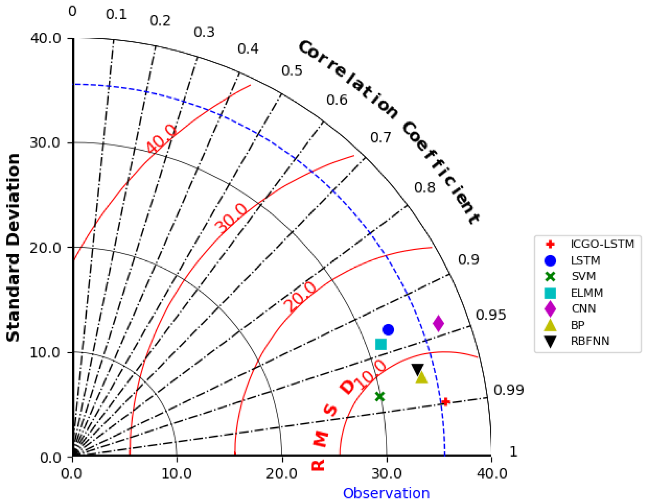
- Simulation results show that compared with seven MH algorithms optimized with LSTM networks, the ICGO-LSTM model obtains the best value in each evaluation index, which proves the effectiveness of the model. Meanwhile, compared with six machine learning algorithms, it can be found that the ICGO-LSTM model still achieves the best evaluation index, which also demonstrates that the model has good prediction performance.
2. Theoretical Approach
2.1. CGO Algorithm
2.2. ICGO Algorithm
2.2.1. Logistic–Sine Mapping Strategy
2.2.2. Q-Learning Strategy
2.2.3. WOA Encircling Prey Mechanism
2.2.4. HEOA Leadership Strategy
| Algorithm 1 ICGO algorithm. |
| Require: Population size , Maximum iterations , dimension variable . Ensure: Optimal solution and optimal function value . Initialize the CGO population according to Equation (7). Calculate the fitness value for each seed. while do for to do Update Q table according to Equation (8), and obtain . Calculate the random factor according to Equation (6). Generate the location of new seed according to Equations (2)–(4). Update the according to Equation (12). end for Boundary check. Calculate the objective function value of the new seed, leaving the one with the better function value compared to the value obtained by the previous seed. for to do Update the locations of seeds according to Equation (14). end for Boundary check. Calculate the objective function value of the updated seed, and if this value is better than the previous one, it is replaced. Update the Q table and obtain . end while return and |
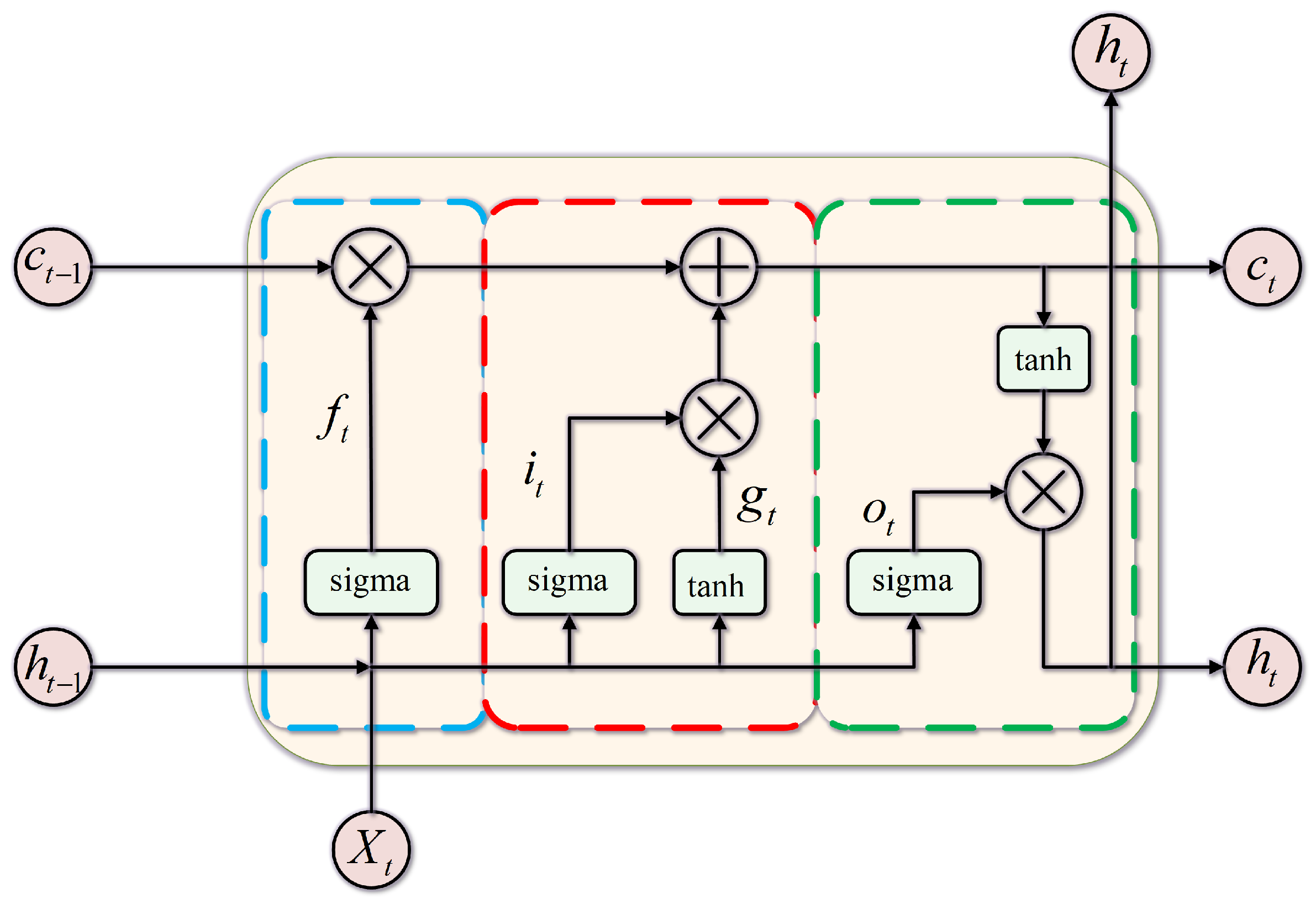
2.3. LSTM Model
2.4. Model Evaluation Index
3. Performance Analysis of the ICGO Algorithm
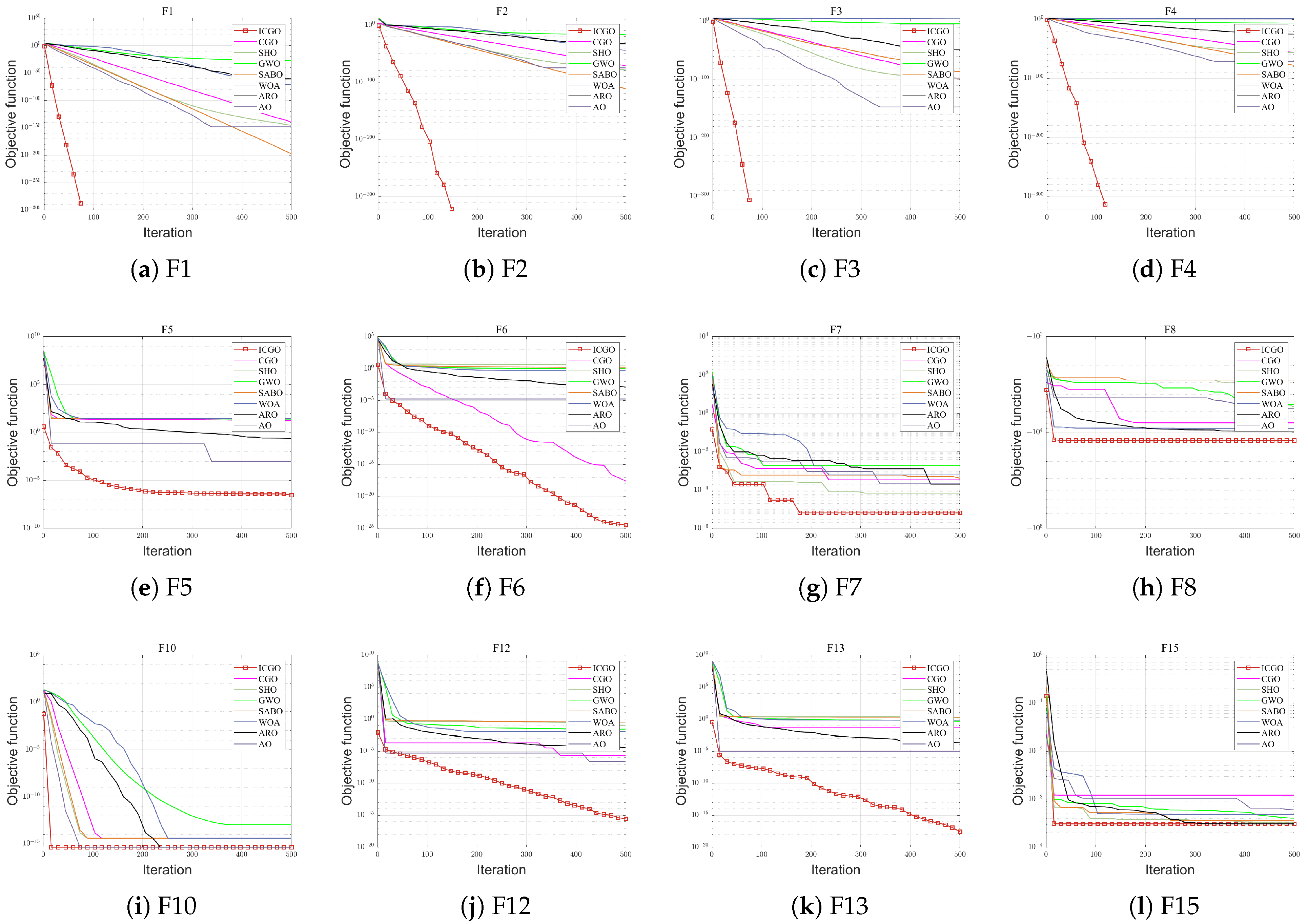
3.1. Test Function
3.2. Analysis of Statistical Results
3.3. Wilcoxon Symbol Test
4. Application of the ICGO-LSTM Model in Air Quality Prediction
4.1. Data Preprocessing
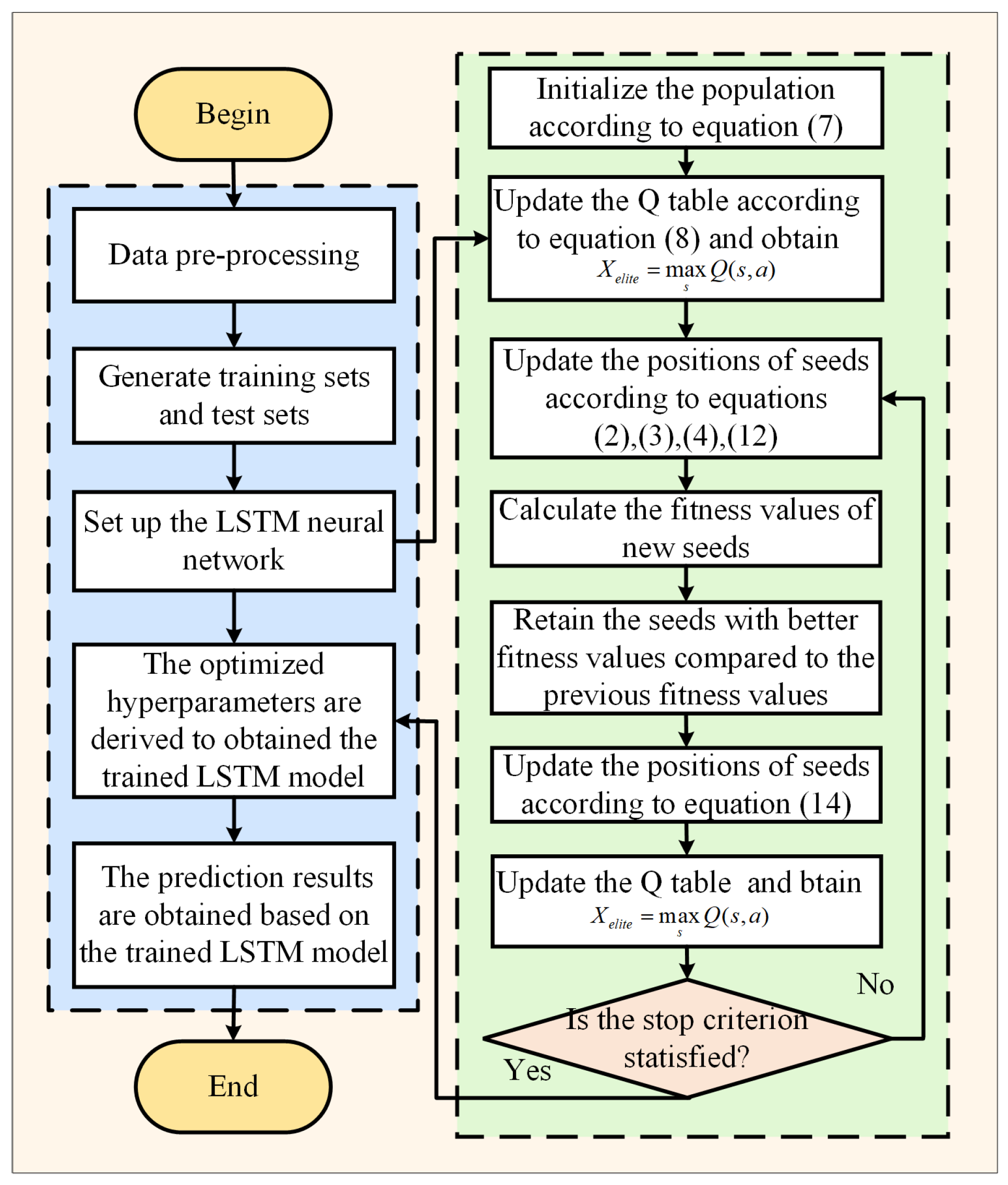
4.2. Establishment of ICGO-LSTM Model
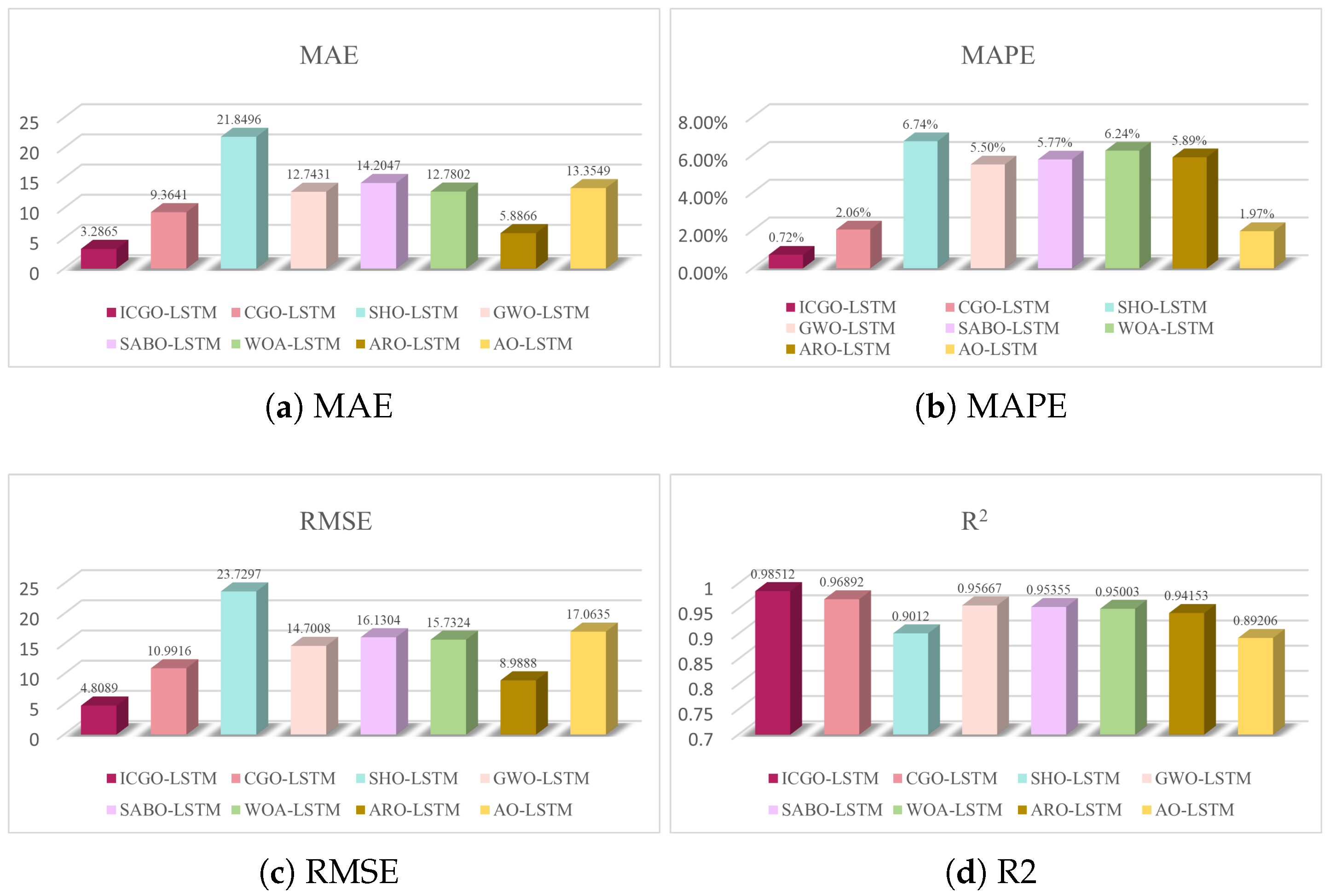
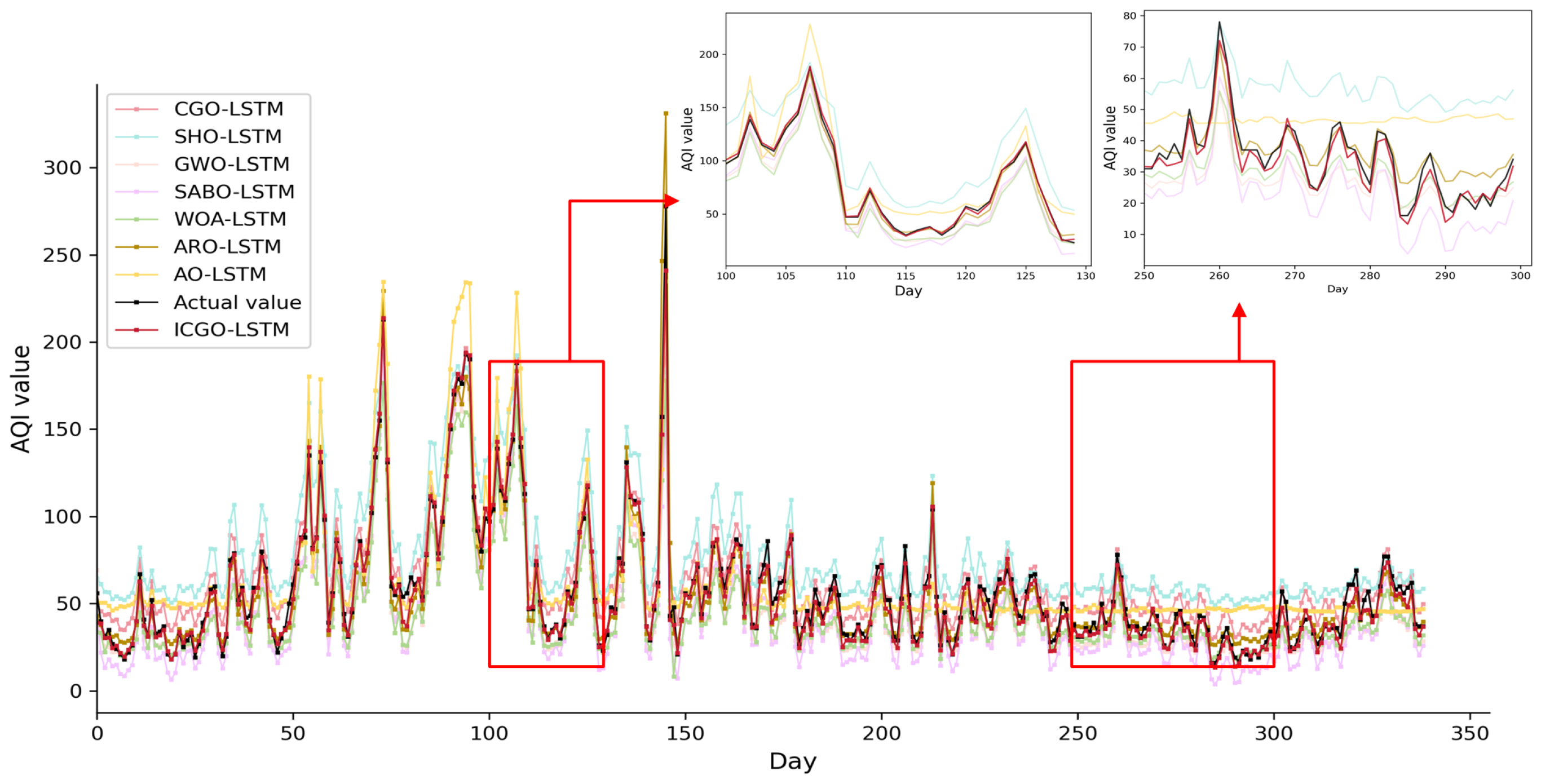
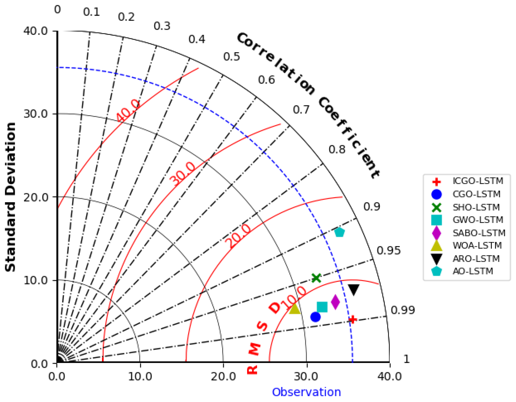
4.3. Comparison of AQI Prediction Results Between ICGO-LSTM and Other MH Algorithms
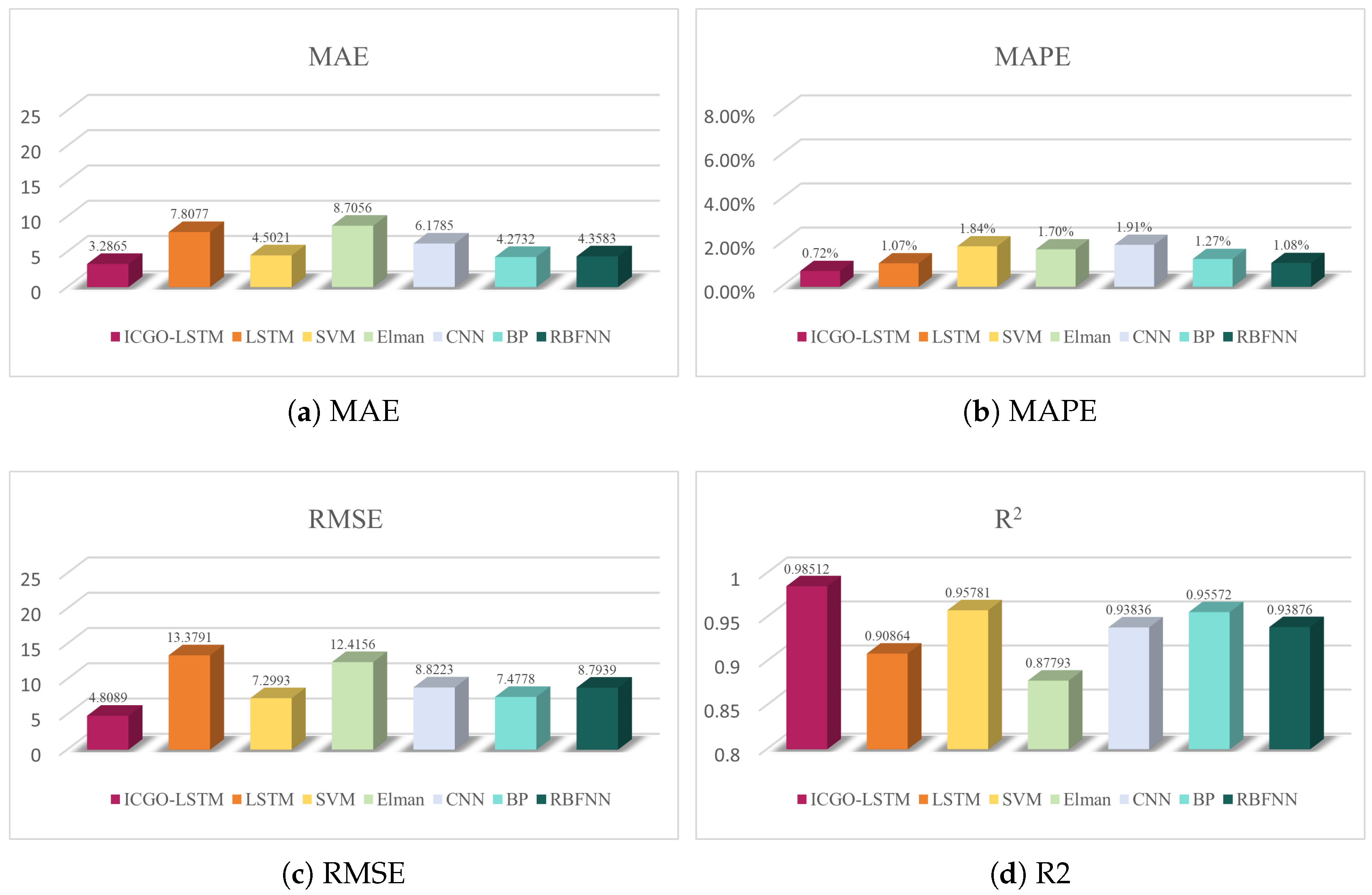
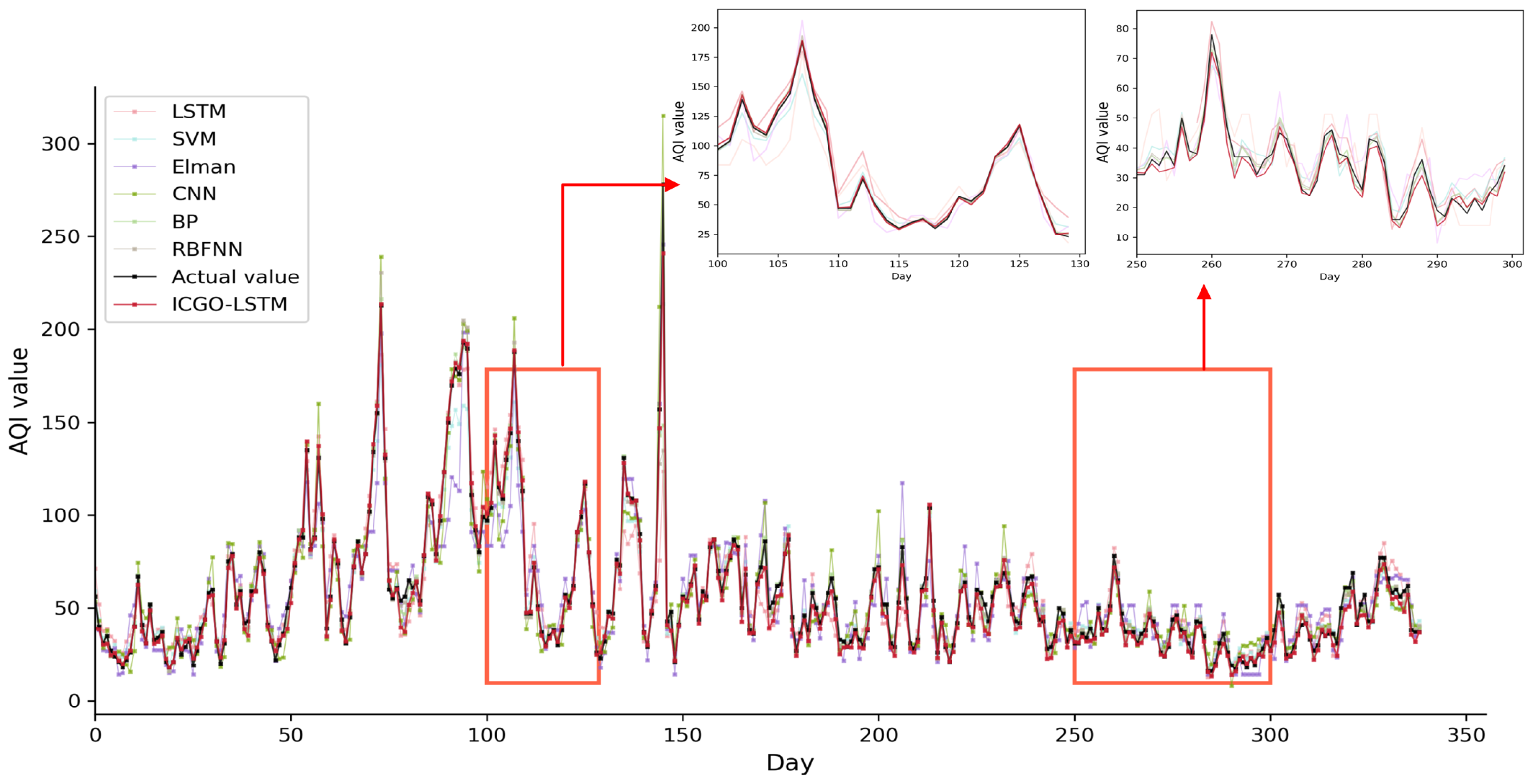
4.4. Comparison of AQI Prediction Results Between ICGO-LSTM Model and Other Machine Learning Methods
5. Conclusions
Author Contributions
Funding
Data Availability Statement
Conflicts of Interest
References
- Tran, V.V.; Park, D.; Lee, Y. Indoor air pollution, related human diseases, and recent trends in the control and improvement of indoor air quality. Int. J. Environ. Res. Public Health 2020, 17, 2927. [Google Scholar] [CrossRef]
- Guo, Z.; Jing, X.; Ling, Y.; Yang, Y.; Jing, N.; Yuan, R.; Liu, Y. Optimized air quality management based on air quality index prediction and air pollutants identification in representative cities in China. Sci. Rep. 2024, 14, 17923. [Google Scholar] [CrossRef]
- Nie, J.; Yu, Z.; Li, J. Multi-objective optimization of the robustness of complex networks based on the mixture of weighted surrogates. Axioms 2023, 12, 404. [Google Scholar] [CrossRef]
- Song, Z.; Deng, Q.; Ren, Z. Correlation and principal component regression analysis for studying air quality and meteorological elements in wuhan, china. Environ. Prog. Sustain. Energy 2020, 39, 13278. [Google Scholar] [CrossRef]
- Mani, G.; Viswanadhapalli, J.K. Prediction and forecasting of air quality index in chennai using regression and arima time series models. J. Eng. Res. 2022, 10, 179–194. [Google Scholar] [CrossRef]
- Syafei, A.D.; Ramadhan, N.; Hermana, J.; Slamet, A.; Boedisantoso, R.; Assomadi, A.F. Application of exponential smoothing holt winter and arima models for predicting air pollutant concentrations. EnvironmentAsia 2018, 11, 251–262. [Google Scholar]
- Janarthanan, R.; Partheeban, P.; Somasundaram, K.; Elamparithi, P.N. A deep learning approach for prediction of air quality index in a metropolitan city. Sustain. Cities Soc. 2021, 67, 102720. [Google Scholar] [CrossRef]
- Gu, Y.; Li, B.; Meng, Q. Hybrid interpretable predictive machine learning model for air pollution prediction. Neurocomputing 2022, 468, 123–136. [Google Scholar] [CrossRef]
- Gupta, N.S.; Mohta, Y.; Heda, K.; Armaan, R.; Valarmathi, B.; Arulkumaran, G. Prediction of air quality index using machine learning techniques: A comparative analysis. J. Environ. Public Health 2023, 2023, 4916267. [Google Scholar] [CrossRef]
- Hardini, M.; Sunarjo, R.A.; Asfi, M.; Chakim, M.H.R.; Sanjaya, Y.P.A. Predicting air quality index using ensemble machine learning. Adi J. Recent Innov. 2023, 5, 78–86. [Google Scholar] [CrossRef]
- Simu, S.; Turkar, V.; Martires, R.; Asolkar, V.; Monteiro, S.; Fernandes, V.; Salgaoncary, V. Air pollution prediction using machine learning. In Proceedings of the 2020 IEEE Bombay Section Signature Conference (IBSSC), Coimbatore, India, 2–4 February 2020; pp. 231–236. [Google Scholar]
- Leong, W.C.; Kelani, R.O.; Ahmad, Z. Prediction of air pollution index (api) using support vector machine(svm). J. Environ. Chem. Eng. 2020, 8, 103208. [Google Scholar]
- Kumar, K.; Pande, B.P. Air pollution prediction with machine learning: A case study of indian cities. Int. J. Environ. Sci. Technol. 2023, 20, 5333–5348. [Google Scholar]
- Guo, Q.; He, Z.; Wang, Z. Prediction of hourly pm2. 5 and pm10 concentrations in chongqing city in china based on artificial neural network. Aerosol Air Qual. Res. 2023, 23, 220448. [Google Scholar]
- Mishra, A.; Gupta, Y. Comparative analysis of air quality index prediction using deep learning algorithms. Spat. Inf. Res. 2024, 32, 63–72. [Google Scholar] [CrossRef]
- Zhang, J.; Li, S. Air quality index forecast in beijing based on cnn-lstm multi-model. Chemosphere 2022, 308, 136180. [Google Scholar]
- Sarkar, N.; Gupta, R.; Keserwani, P.K.; Govil, M.C. Air quality index prediction using an effective hybrid deep learning model. Environ. Pollut. 2022, 315, 120404. [Google Scholar]
- Kim, D.; Han, H.; Wang, W.; Kang, Y.; Lee, H.; Kim, H.S. Application of deep learning models and network method for comprehensive air-quality index prediction. Appl. Sci. 2022, 12, 6699. [Google Scholar] [CrossRef]
- Bacanin, N.; Stoean, C.; Zivkovic, M.; Rakic, M.; Strulak-Wójcikiewicz, R.; Stoean, R. On the benefits of using metaheuristics in the hyperparameter tuning of deep learning models for energy load forecasting. Energies 2023, 16, 1434. [Google Scholar] [CrossRef]
- Chakraborty, S.; Saha, A.K.; Sharma, S.; Chakraborty, R.; Debnath, S. A hybrid whale optimization algorithm for global optimization. J. Ambient. Intell. Humaniz. Comput. 2023, 14, 431–467. [Google Scholar]
- Dehghani, M.; Trojovskỳ, P. Osprey optimization algorithm: A new bio-inspired metaheuristic algorithm for solving engineering optimization problems. Front. Mech. Eng. 2023, 8, 1126450. [Google Scholar]
- Huang, Y.; Yu, J.; Dai, X.; Huang, Z.; Li, Y. Air-quality prediction based on the md–ipso–lstm combination model. Sustainability 2022, 14, 4889. [Google Scholar]
- Nguyen, A.T.; Pham, D.H.; Oo, B.L.; Ahn, Y.; Lim, B.T.H. Predicting air quality index using attention hybrid deep learning and quantum-inspired particle swarm optimization. J. Big Data 2024, 11, 71. [Google Scholar]
- Drewil, G.I.; Al-Bahadili, R.J. Air pollution prediction using lstm deep learning and metaheuristics algorithms. Meas. Sens. 2022, 24, 100546. [Google Scholar]
- Baniasadi, S.; Salehi, R.; Soltani, S.; Martín, D.; Pourmand, P.; Ghafourian, E. Optimizing long short-term memory network for air pollution prediction using a novel binary chimp optimization algorithm. Electronics 2023, 12, 3985. [Google Scholar] [CrossRef]
- Duan, J.; Gong, Y.; Luo, J.; Zhao, Z. Air-quality prediction based on the arima-cnn-lstm combination model optimized by dung beetle optimizer. Sci. Rep. 2023, 13, 12127. [Google Scholar]
- Wang, S.; Li, P.; Ji, H.; Zhan, Y.; Li, H. Prediction of air particulate matter in Beijing, China, based on the improved particle swarm optimization algorithm and long short-term memory neural network. J. Intell. Fuzzy Syst. 2021, 41, 1869–1885. [Google Scholar]
- Li, J.; Chen, J.; Shi, J. Evaluation of new sparrow search algorithms with sequential fusion of improvement strategies. Comput. Ind. Eng. 2023, 182, 109425. [Google Scholar] [CrossRef]
- Zhao, X.; Chen, Y.; Wei, G.; Pang, L.; Xu, C. A comprehensive compensation method for piezoresistive pressure sensor based on surface fitting and improved grey wolf algorithm. Measurement 2023, 207, 112387. [Google Scholar]
- Duan, Y.; Yu, X. A collaboration-based hybrid gwo-sca optimizer for engineering optimization problems. Expert Syst. Appl. 2023, 213, 119017. [Google Scholar]
- Talatahari, S.; Azizi, M. Chaos game optimization: A novel metaheuristic algorithm. Artif. Intell. Rev. 2021, 54, 917–1004. [Google Scholar]
- Alam, A.; Muqeem, M. An optimal heart disease prediction using chaos game optimization-based recurrent neural model. Int. J. Inf. Technol. 2024, 16, 3359–3366. [Google Scholar] [CrossRef]
- Goodarzimehr, V.; Talatahari, S.; Shojaee, S.; Hamzehei-Javaran, S.; Sareh, P. Structural design with dynamic constraints using weighted chaos game optimization. J. Comput. Des. Eng. 2022, 9, 2271–2296. [Google Scholar] [CrossRef]
- Shaheen, M.A.M.; Hasanien, H.M.; Mekhamer, S.F.; Talaat, H.E.A. A chaos game optimization algorithm-based optimal control strategy for performance enhancement of offshore wind farms. Renew. Energy Focus 2024, 49, 100578. [Google Scholar] [CrossRef]
- Özbay, F.A. A modified seahorse optimization algorithm based on chaotic maps for solving global optimization and engineering problems. Eng. Sci. Technol. Int. J. 2023, 41, 101408. [Google Scholar] [CrossRef]
- Hsieh, C.; Zhang, Q.; Xu, Y.; Wang, Z. Cmais-woa: An improved woa with chaotic mapping and adaptive iterative strategy. Discret. Dyn. Nat. Soc. 2023, 2023, 8160121. [Google Scholar] [CrossRef]
- Hu, Z.; Yu, X. Reinforcement learning-based comprehensive learning grey wolf optimizer for feature selection. Appl. Soft Comput. 2023, 149, 110959. [Google Scholar] [CrossRef]
- Gao, X.; Zhou, Y.; Xu, L.; Zhao, D. Optimal Security Protection Strategy Selection Model Based on Q-Learning Particle Swarm Optimization. Entropy 2022, 24, 1727. [Google Scholar] [CrossRef]
- Lian, J.; Hui, G. Human evolutionary optimization algorithm. Expert Syst. Appl. 2024, 241, 122638. [Google Scholar]
- Cheng, M.; Zhang, Q.; Cao, Y. An early warning model for turbine intermediate-stage flux failure based on an improved heoa algorithm optimizing dmse-gru model. Energies 2024, 17, 3629. [Google Scholar] [CrossRef]
- Song, Q.; Zou, J.; Xu, M.; Xi, M.; Zhou, Z. Air quality prediction for chengdu based on long short-term memory neural network with improved jellyfish search optimizer. Environ. Sci. Pollut. Res. 2023, 30, 64416–64442. [Google Scholar] [CrossRef]
- Chang, Y.; Chiao, H.; Abimannan, S.; Huang, Y.P.; Tsai, Y.T.; Lin, K. An lstm-based aggregated model for air pollution forecasting. Atmos. Pollut. Res. 2020, 11, 1451–1463. [Google Scholar] [CrossRef]
- Wang, J.; Li, J.; Wang, X.; Wang, J.; Huang, M. Air quality prediction using ct-lstm. Neural Comput. Appl. 2021, 33, 4779–4792. [Google Scholar] [CrossRef]
- Zhao, S.; Zhang, T.; Ma, S.; Wang, M. Sea-horse optimizer: A novel nature-inspired meta-heuristic for global optimization problems. Appl. Intell. 2023, 53, 11833–11860. [Google Scholar] [CrossRef]
- Trojovskỳ, P.; Dehghani, M. Subtraction-average-based optimizer: A new swarm-inspired metaheuristic algorithm for solving optimization problems. Biomimetics 2023, 8, 149. [Google Scholar] [CrossRef] [PubMed]
- Wang, L.; Cao, Q.; Zhang, Z.; Mirjalili, S.; Zhao, W. Artificial rabbits optimization: A new bio-inspired meta-heuristic algorithm for solving engineering optimization problems. Eng. Appl. Artif. Intell. 2022, 114, 105082. [Google Scholar] [CrossRef]
- Abualigah, L.; Yousri, D.; Elaziz, M.A.; Ewees, A.A.; Al-Qaness, M.A.; Gandomi, A.H. Aquila optimizer: A novel meta-heuristic optimization algorithm. Comput. Ind. Eng. 2021, 157, 107250. [Google Scholar] [CrossRef]
- Abdullah, D.M.; Abdulazeez, A.M. Machine learning applications based on svm classification a review. Qubahan Acad. J. 2021, 1, 81–90. [Google Scholar] [CrossRef]
- Guo, Y.; Yang, D.; Zhang, Y.; Wang, L.; Wang, K. Online estimation of soh for lithium-ion battery based on ssa-elman neural network. Prot. Control Mod. Power Syst. 2022, 7, 40. [Google Scholar] [CrossRef]
- Yan, R.; Liao, J.; Yang, J.; Sun, W.; Nong, M.; Li, F. Multi-hour and multi-site air quality index forecasting in beijing using cnn, lstm, cnn-lstm, and spatiotemporal clustering. Expert Syst. Appl. 2021, 169, 114513. [Google Scholar] [CrossRef]
- Huang, Y.; Xiang, Y.; Zhao, R.; Cheng, Z. Air quality prediction using improved pso-bp neural network. IEEE Access 2020, 8, 99346–99353. [Google Scholar] [CrossRef]
- Du, J. Mechanism analysis and self-adaptive rbfnn based hybrid soft sensor model in energy production process: A case study. Sensors 2022, 22, 1333. [Google Scholar] [CrossRef] [PubMed]


| Function | Range | Dim | fmin |
|---|---|---|---|
| [−100,100] | 30 | 0 | |
| [−10,10] | 30 | 0 | |
| [−100,100] | 30 | 0 | |
| [−100,100] | 30 | 0 | |
| [−30,30] | 30 | 0 | |
| [−100,100] | 30 | 0 | |
| [−1.28,1.28] | 30 | 0 | |
| [−500,500] | 30 | −12,569.5 | |
| [−5.12,5.12] | 30 | 0 | |
| [−32,32] | 30 | 0 | |
| [−600,600] | 30 | 0 | |
| [−50,50] | 30 | 0 | |
| [−50,50] | 30 | 0 | |
| [−65,65] | 2 | 1 | |
| [−5,5] | 4 | 0.000308 | |
| [−5,5] | 2 | −1.0316 | |
| [−5,10],[0,15] | 2 | 0.398 | |
| [−2,2] | 2 | 3 | |
| [0,1] | 3 | −3.86 | |
| [0,1] | 6 | −3.32 | |
| [0,10] | 4 | −10.15 | |
| [0,10] | 4 | −10.4 | |
| [0,10] | 4 | −10.536 |
| Algorithm | Parameters | Value |
|---|---|---|
| CGO | , | A random integer of 0 or 1 |
| R | [0,1] | |
| SHO | 0 | |
| 0.1 | ||
| GWO | Linear reduction from 2 to 0 | |
| SABO | v | [1,2] |
| WOA | 0.1 | |
| r, l | [0,1],[−1,1] | |
| ARO | , , | [0,1] |
| AO | [1,20] | |
| v | 0.0265 | |
| w | 0.005 |
| Function | ICGO | CGO | SHO | GWO | SABO | WOA | ARO | AO | Index |
|---|---|---|---|---|---|---|---|---|---|
| F1 | 0.00 | 8.15 | 1.49 | 9.45 | 3.10 | 2.08 | 3.40 | 3.66 | avg |
| 0.00 | 1.53 | 4.83 | 1.49 | 0.00 | 5.53 | 1.04 | 1.16 | std | |
| F2 | 0.00 | 1.81 | 1.17 | 8.05 | 5.86 | 1.31 | 1.12 | 2.37 | avg |
| 0.00 | 2.21 | 1.83 | 8.54 | 1.80 | 3.53 | 3.54 | 7.50 | std | |
| F3 | 0.00 | 1.18 | 5.26 | 1.50 | 2.06 | 4.24 | 7.33 | 3.65 | avg |
| 0.00 | 3.54 | 9.17 | 3.02 | 9.21 | 1.51 | 2.32 | 1.15 | std | |
| F4 | 0.00 | 1.18 | 2.91 | 5.64 | 1.34 | 4.41 | 8.55 | 7.45 | avg |
| 0.00 | 1.59 | 1.18 | 7.70 | 1.69 | 3.19 | 1.27 | 2.35 | std | |
| F5 | 1.77 | 2.53 | 2.81 | 2.71 | 2.84 | 2.78 | 3.17 | 4.66 | avg |
| 4.95 | 5.74 | 2.89 | 2.85 | 2.88 | 4.22 | 8.13 | 5.22 | std | |
| F6 | 7.43 | 3.73 | 3.17 | 8.81 | 2.73 | 3.49 | 1.35 | 2.82 | avg |
| 3.57 | 2.00 | 5.53 | 3.67 | 5.23 | 1.84 | 7.09 | 3.07 | std | |
| F7 | 3.21 | 1.41 | 8.30 | 6.39 | 6.43 | 2.93 | 8.73 | 1.06 | avg |
| 5.39 | 6.82 | 8.94 | 1.15 | 8.79 | 3.46 | 5.29 | 9.41 | std | |
| F8 | −1.08 | −7.98 | −6.02 | −5.84 | −3.18 | −1.01 | −9.21 | −9.04 | avg |
| 1.07 | 4.37 | 6.37 | 9.33 | 3.45 | 1.93 | 3.87 | 3.90 | std | |
| F9 | 0.00 | 0.00 | 0.00 | 3.82 | 0.00 | 5.68 | 0.00 | 0.00 | avg |
| 0.00 | 0.00 | 0.00 | 4.22 | 0.00 | 2.54 | 0.00 | 0.00 | std | |
| F10 | 4.44 | 1.96 | 4.00 | 9.92 | 4.00 | 3.46 | 4.44 | 4.44 | avg |
| 0.00 | 3.58 | 0.00 | 1.73 | 0.00 | 2.38 | 0.00 | 0.00 | std | |
| F11 | 0.00 | 0.00 | 0.00 | 7.06 | 0.00 | 1.18 | 0.00 | 0.00 | avg |
| 0.00 | 0.00 | 0.00 | 1.09 | 0.00 | 5.29 | 0.00 | 0.00 | std | |
| F12 | 2.08 | 7.40 | 9.52 | 3.84 | 2.19 | 1.13 | 8.94 | 1.15 | avg |
| 6.84 | 2.63 | 7.79 | 1.58 | 8.59 | 3.80 | 6.10 | 1.03 | std | |
| F13 | 7.95 | 2.36 | 1.95 | 5.56 | 2.75 | 5.51 | 2.83 | 6.62 | avg |
| 3.05 | 5.46 | 3.27 | 2.26 | 5.49 | 2.75 | 4.70 | 9.29 | std | |
| F14 | 9.98 | 2.24 | 5.11 | 4.98 | 3.23 | 2.61 | 9.98 | 1.89 | avg |
| 0.00 | 2.54 | 4.29 | 4.53 | 1.80 | 2.39 | 0.00 | 8.69 | std | |
| F15 | 3.07 | 5.69 | 5.09 | 4.37 | 1.27 | 7.70 | 4.49 | 4.65 | avg |
| 1.94 | 9.00 | 3.57 | 8.21 | 2.83 | 5.11 | 2.97 | 9.08 | std | |
| F16 | −1.03 | −1.03 | −1.03 | −1.03 | −1.02 | −1.03 | −1.03 | −1.03 | avg |
| 5.78 | 6.25 | 7.33 | 1.59 | 1.94 | 1.09 | 1.28 | 7.25 | std | |
| F17 | 3.98 | 3.98 | 3.98 | 3.98 | 5.21 | 3.98 | 3.98 | 3.98 | avg |
| 0.00 | 0.00 | 1.28 | 1.50 | 2.09 | 3.67 | 0.00 | 2.47 | std | |
| F18 | 3.00 | 3.00 | 3.00 | 3.00 | 4.17 | 3.00 | 0.00 | 3.03 | avg |
| 8.25 | 4.73 | 5.16 | 2.35 | 2.15 | 2.66 | 3.31 | 3.86 | std | |
| F19 | −3.86 | −3.86 | −3.86 | −3.86 | −3.65 | −3.86 | −3.86 | −3.86 | avg |
| 2.51 | 2.58 | 3.80 | 2.19 | 1.86 | 5.09 | 9.36 | 6.41 | std | |
| F20 | −3.32 | −3.25 | −3.03 | −3.26 | −3.26 | −3.20 | −3.25 | −3.20 | avg |
| 1.36 | 3.92 | 2.04 | 7.74 | 8.00 | 6.07 | 6.14 | 2.00 | std | |
| F21 | −1.15 | −7.38 | −5.85 | −9.65 | −5.04 | −8.74 | −9.64 | −1.01 | avg |
| 7.17 | 3.12 | 2.47 | 1.56 | 1.64 | 2.52 | 1.61 | 9.11 | std | |
| F22 | −1.04 | −7.59 | −5.32 | −1.00 | −4.94 | −6.57 | −9.20 | −1.04 | avg |
| 1.78 | 3.36 | 1.94 | 1.71 | 3.72 | 2.97 | 2.55 | 9.13 | std | |
| F23 | −1.05 | −8.39 | −5.62 | −1.01 | −4.69 | −6.93 | −9.33 | −1.05 | avg |
| 7.38 | 2.93 | 1.88 | 1.81 | 1.25 | 3.28 | 2.57 | 1.47 | std |
| Function | ICGO vs. CGO | ICGO vs. SHO | ICGO vs. GWO | ICGO vs. SABO | ICGO vs. WOA | ICGO vs. ARO | ICGO vs. AO | Index |
|---|---|---|---|---|---|---|---|---|
| F1 | 6.25 | 1.21 | 1.21 | 1.01 | 1.21 | 2.21 | 2.01 | p |
| F2 | 4.57 | 1.01 | 1.61 | 1.16 | 1.21 | 2.11 | 1.81 | p |
| F3 | 1.21 | 1.51 | 1.11 | 1.01 | 1.51 | 1.27 | 1.27 | p |
| F4 | 1.93 | 1.71 | 1.41 | 1.27 | 2.21 | 1.61 | 3.21 | p |
| F5 | 3.02 | 1.02 | 3.02 | 3.02 | 3.02 | 3.02 | 3.02 | p |
| F6 | 3.02 | 3.18 | 3.09 | 3.12 | 2.02 | 1.32 | 2.02 | p |
| F7 | 3.34 | 1.49 | 3.12 | 2.44 | 3.02 | 3.69 | 3.59 | p |
| F8 | 2.28 | 3.02 | 3.02 | 3.02 | 7.28 | 7.28 | 7.28 | p |
| F9 | NAN | NAN | 1.20 | NAN | 1.61 | NAN | NAN | p |
| F10 | 5.59 | 1.17 | 1.12 | 1.69 | 7.75 | NAN | NAN | p |
| F11 | NAN | NAN | 2.15 | NAN | 3.34 | NAN | NAN | p |
| F12 | 2.02 | 3.02 | 3.02 | 3.02 | 3.02 | 2.02 | 1.02 | p |
| F13 | 1.07 | 3.02 | 3.02 | 3.02 | 3.02 | 4.02 | 2.02 | p |
| F14 | 5.32 | 4.71 | 1.00 | 1.29 | 2.02 | 1.49 | 3.71 | p |
| F15 | 2.90 | 3.46 | 1.61 | 3.46 | 3.46 | 4.37 | 5.56 | p |
| F16 | 6.72 | 5.36 | 5.36 | 5.36 | 5.36 | 2.23 | 5.36 | p |
| F17 | 3.30 | 2.80 | 2.80 | 2.80 | 2.80 | 3.30 | 2.80 | p |
| F18 | 1.80 | 1.43 | 1.43 | 1.43 | 1.43 | 1.22 | 1.43 | p |
| F19 | 2.23 | 1.91 | 2.26 | 2.40 | 1.68 | 6.00 | 2.19 | p |
| F20 | 2.09 | 3.87 | 2.02 | 1.44 | 1.73 | 4.32 | 1.15 | p |
| F21 | 3.44 | 1.53 | 1.53 | 1.53 | 1.13 | 3.18 | 1.53 | p |
| F22 | 2.11 | 1.60 | 1.60 | 1.60 | 1.60 | 2.39 | 2.60 | p |
| F23 | 1.69 | 1.74 | 1.94 | 1.31 | 1.24 | 1.57 | 1.74 | p |
| Total | 21/2/0 | 21/2/0 | 23/0/0 | 21/2/0 | 23/0/0 | 20/3/0 | 20/3/0 |
| Model | MAE | MAPE | RMSE | R2 | Running Time (s) |
|---|---|---|---|---|---|
| ICGO-LSTM | 3.2865 | 0.72% | 4.8089 | 0.98512 | 880 |
| CGO-LSTM | 9.3641 | 2.06% | 10.9916 | 0.96892 | 1040 |
| SHO-LSTM | 21.8496 | 6.74% | 23.7297 | 0.9012 | 1186 |
| GWO-LSTM | 12.7431 | 5.50% | 14.7008 | 0.95667 | 925 |
| SABO-LSTM | 14.2047 | 5.77% | 16.1304 | 0.95355 | 1185 |
| WOA-LSTM | 12.7802 | 6.24% | 15.7324 | 0.95003 | 1021 |
| ARO-LSTM | 5.8866 | 5.89% | 8.9888 | 0.94153 | 972 |
| AO-LSTM | 13.3549 | 1.97% | 17.0635 | 0.89206 | 1208 |
| Model | MAE | MAPE | RMSE | R2 | Running Time (s) |
|---|---|---|---|---|---|
| ICGO-LSTM | 3.2865 | 0.72% | 4.8089 | 0.98512 | 880 |
| LSTM | 7.8077 | 1.07% | 13.3791 | 0.90864 | 23 |
| SVM | 4.5021 | 1.84% | 7.2993 | 0.95781 | 10 |
| Elman | 8.7056 | 1.70% | 12.4156 | 0.87793 | 19 |
| CNN | 6.1785 | 1.91% | 8.8223 | 0.93836 | 16 |
| BP | 4.2732 | 1.27% | 7.4778 | 0.95572 | 20 |
| RBFNN | 4.3583 | 1.08% | 8.7939 | 0.93876 | 18 |
Disclaimer/Publisher’s Note: The statements, opinions and data contained in all publications are solely those of the individual author(s) and contributor(s) and not of MDPI and/or the editor(s). MDPI and/or the editor(s) disclaim responsibility for any injury to people or property resulting from any ideas, methods, instructions or products referred to in the content. |
© 2025 by the authors. Licensee MDPI, Basel, Switzerland. This article is an open access article distributed under the terms and conditions of the Creative Commons Attribution (CC BY) license (https://creativecommons.org/licenses/by/4.0/).
Share and Cite
Liu, Y.; Zheng, R.; Yu, B.; Liao, B.; Song, F.; Tang, C. An Improved Chaotic Game Optimization Algorithm and Its Application in Air Quality Prediction. Axioms 2025, 14, 235. https://doi.org/10.3390/axioms14040235
Liu Y, Zheng R, Yu B, Liao B, Song F, Tang C. An Improved Chaotic Game Optimization Algorithm and Its Application in Air Quality Prediction. Axioms. 2025; 14(4):235. https://doi.org/10.3390/axioms14040235
Chicago/Turabian StyleLiu, Yanping, Rongyan Zheng, Bohao Yu, Bin Liao, Fuhong Song, and Chunju Tang. 2025. "An Improved Chaotic Game Optimization Algorithm and Its Application in Air Quality Prediction" Axioms 14, no. 4: 235. https://doi.org/10.3390/axioms14040235
APA StyleLiu, Y., Zheng, R., Yu, B., Liao, B., Song, F., & Tang, C. (2025). An Improved Chaotic Game Optimization Algorithm and Its Application in Air Quality Prediction. Axioms, 14(4), 235. https://doi.org/10.3390/axioms14040235