Classification of the Second Minimal Orbits in the Sharkovski Ordering

Abstract

We prove a conjecture on the second minimal odd periodic orbits with respect to Sharkovski ordering for the continuous endomorphisms on the real line. A $(2k+1)$-periodic orbit $\{{\beta }_1<{\beta }_2<\cdots <{\beta }_{2k+1}\}$, ($k\ge 3$) is called second minimal for the map f, if $2k-1$ is a minimal period of ${f|}_{[{\beta }_1,{\beta }_{2k+1}]}$ in the Sharkovski ordering. Full classification of second minimal orbits is presented in terms of cyclic permutations and directed graphs of transitions. It is proved that second minimal odd orbits either have a Stefan-type structure like minimal odd orbits or one of the $4k-3$ types, each characterized with unique cyclic permutations and directed graphs of transitions with an accuracy up to the inverses. The new concept of second minimal orbits and its classification have an important application towards an understanding of the universal structure of the distribution of the periodic windows in the bifurcation diagram generated by the chaotic dynamics of nonlinear maps on the interval.

1. Introduction

Let $f:I\to I$ be a continuous endomorphism, and I be a non-degenerate interval on the real line. Let $f^n:I\to I$ be an n-th iteration of f. A point $c\in I$ is called a periodic point of f with period m if $f^m\left(c\right)=c$, $f^k\left(c\right)\ne c$ for $1\le k<m$. The set of m distinct points

$$c,f\left(c\right),\cdots ,f^{m-1}\left(c\right)$$

is called the orbit of c, or briefly, an m-orbit or periodic m-cycle. In their celebrated paper [1], Sharkovski discovered a law on the coexistence of periodic orbits of continuous endomorphisms on the real line.

Theorem 1 

([1]). Let the positive integers be totally ordered in the following way:

$$1◃2◃2^2◃2^3◃\cdots ◃2^2·5◃2^2·3◃\cdots ◃2·5◃2·3◃\cdots ◃9◃7◃5◃3.$$

(1)

If a continuous endomorphism, $f:I\to I$, has a cycle of period n and $m◃n$, then f also has a periodic orbit of period m.

This result played a fundamental role in the development of the theory of discrete dynamical systems [2,3,4]. Following the standard approach ([2,5]), we characterize each periodic orbit with cyclic permutations and directed graphs of transitions or digraphs. Consider the m-orbit:

$$\mathbf{B}=\{{\beta }_1<{\beta }_2<\cdots <{\beta }_m\}$$

Definition 1. 

If $f\left({\beta }_i\right)={\beta }_{s_i}$ for $1\le s_i\le m$, with $i=1,2,\cdots ,m$, then $\mathbf{B}$ is associated with the cyclic permutation

$$\pi =\left(\begin{array}{cccc}1& 2& \cdots & m\\ s_1& s_2& \cdots & s_m\end{array}\right)$$

In the sequel, $<a,b>$ means either $[a,b]$ or $[b,a]$.

Definition 2. 

Let $J_i=[{\beta }_i,{\beta }_{i+1}]$. The digraph of the m-orbit is a directed graph of transitions with vertices $J_1,J_2,\cdots ,J_{m-1}$ and oriented edges $J_i\to J_s$ if $J_s\subset <f\left({\beta }_i\right),f\left({\beta }_{i+1}\right)>$.

Definition 3. 

The inverse digraph of the m-orbit is obtained from the digraph of the m-orbit by replacing each $J_i$ with $J_{m-i}$.

The inverse of the digraph associated with the cyclic permutation $\pi$ is a digraph associated with the cyclic permutation $\omega \circ \pi \circ \omega$, where $\omega$ is the order-reversing permutation:

$$\omega =\left(\begin{array}{ccccc}1& 2& \dots & m-1& m\\ m& m-1& \dots & 2& 1\end{array}\right)$$

Definition 4. 

A continuous function $P_f:\left[{\beta }_1,{\beta }_m\right]\to \left[{\beta }_1,{\beta }_m\right]$ is called the P-linearization of f if $P_f\left({\beta }_i\right)=f\left({\beta }_i\right)$ and P is a linear function in each interval $J_i$

Definition 5. 

The arrangement of the minimums and maximums of the map $P_f$ in the open interval $\left({\beta }_1,{\beta }_m\right)$ will be called the topological structure of the periodic orbit.

The proof of Sharkovski’s theorem significantly uses the concept of a minimal orbit.

Definition 6. 

The m-orbit of f is called minimal if m is the minimal period of ${f|}_{[{\beta }_1,{\beta }_m]}$ in the Sharkovski ordering.

Definition 7. 

The digraph of the m-orbit contains the red edge J_i→J_s if $J_s=<f\left({\beta }_i\right),f\left({\beta }_{i+1}\right)>$.

The structure of minimal orbits is well understood [2,6,7,8,9,10]. Minimal odd orbits are called Stefan orbits, due to the following characterization:

Theorem 2 

([6]). The digraph of a minimal $2k+1$-orbit, $k\ge 1$, has the unique structure given in Figure 1 and cyclic permutation (2) up to an inverse.

$$\left(\begin{array}{ccccccccccc}1& 2& 3& \cdots & k& k+1& k+2& k+3& \cdots & 2k& 2k+1\\ k+1& 2k+1& 2k& \cdots & k+3& k+2& k& k-1& \cdots & 2& 1\end{array}\right)$$

(2)

2. Main Results

The main goal of this paper is the characterization of second minimal odd orbits.

Definition 8. 

A $(2k+1)$-orbit, $k\ge 3$ is called second minimal if $2k-1$ is the minimal period of ${f|}_{[{\beta }_1,{\beta }_{2k+1}]}$ in the Sharkovski ordering.

To achieve the full characterization of second minimal odd orbits, in the next definition, we introduce a new notion of the simplicity of odd periodic orbits. Let $B(i,j)$, $1\le i\le j\le 2k+1$ be subsets of a $(2k+1)$-orbit defined as

$$B(i,j)=\left\{{\beta }_k\in B:i\le k\le j\right\}$$

(3)

Definition 9. 

A $(2k+1)$-orbit is called simple if either

1. 

$B(k+2,2k+1)$ is mapped to $B(1,k+1)$; and $B(1,k+1)$ is mapped to $B(k+2,2k+1)$ except for one point; or

2. 

$B(1,k)$ is mapped to $B(k+1,2k+1)$; and $B(k+1,2k+1)$ is mapped to $B(1,k)$ except for one point.

We say a simple $(2k+1)$-orbit is of type + (resp. type −) if (1) (resp. (2)) is satisfied.

First of all, note that the Stefan orbits or minimal odd orbits are simple according to Definition 9. Our first main result reads:

Theorem 3. 

Second minimal $(2k+1)$-orbits, $k\ge 3$, are simple.

To pursue a full classification of second minimal odd orbits, first note that second minimal odd orbits may have a Stefan structure as identified in Theorem 2. Indeed, consider a map that is the P-linearization of the minimal $2k+1$-orbit. It has a unique fixed point that is an interior point of one of the two middle intervals. We can replace the linear function in the small neighborhood F of the fixed point with a P-linearization of the minimal $2k-1$-orbit and join this function continuously with the original map outside of the small neighborhood of a size twice that of F. Moreover, we can choose the size of F to be so small that the digraph of the $2k+1$-orbit is not changed and still has a Stefan structure. Obviously, the $2k+1$-orbit is second minimal with respect to the new map, although its Stefan structure is unchanged. Therefore, to complete the full classification, it remains to clarify the structure of all second minimal odd orbits with a non-Stefan structure. Our main classification result reads:

Theorem 4. 

Simple positive-type second minimal $2k+1$-orbits are either Stefan orbits or have one of the $4k-3$ types, each with a unique digraph and cyclic permutation. Their inverses represent all second minimal $(2k+1)$-orbits of the simple negative type. The topological structure of all $4k-3$ simple positive types of second minimal $(2k+1)$-orbits with a non-Stefan structure is presented in

Table 1. Topological structure of all $4k-3$ second minimal $(2k+1)$-orbits of the simple positive type with a non-Stefan structure.

Topological Structure	Count
max	1
min-max	1
min-max-min	1
max-min	2
max-min-max	$2k-3$
max-min-max-min-max	$2k-5$

. The topological structure of their inverses is obtained by replacing “max” and “min” with each other. The P-linearization of each of the $4k-3$ types (and their inverses) presents an example of a continuous map with a second minimal $(2k+1)$-orbit.

Theorems 3 and 4 in the particular case $k=3$ were proved in [11]. The proof of Theorems 3 and 4 is constructive, and provides explicit description of all types of second minimal odd orbits in terms of cyclic permutations and digraphs. Second minimal orbits play an important role in the problem on the distribution of periodic windows within the chaotic regime of the bifurcation diagram of the one-parameter family of unimodal maps dependent on a parameter. For example, consider an iterative relation $x_{n+1}=f_{\lambda }\left(x_n\right)$, where the maps $f_{\lambda }:[0,1]\to [0,1]$ satisfy $f\left(0\right)=f\left(1\right)=0$ with a single maximum at some point, $x_{max}$, interior to the interval $[0,1]$. The problem is to comprehend a full characterization of the asymptotic behavior of $x_n$ for $n\to \infty$ and how this behavior depends on the parameter $\lambda$. A prototypical example is the logistic map

$$x_{n+1}=4\lambda x_n\left(1-x_n\right)$$

(4)

In 1978, Fiegenbaum [12,13,14] discovered a universal transition mechanism to chaos through successive period doubling bifurcations. As $\lambda \uparrow {\lambda }_{\infty }$, with some transition value ${\lambda }_{\infty }<1$, the behavior of $x_n$ for large n changes from periodic to chaotic via bifurcations from the $2^n$ periodic cycle to the $2^{n+1}$ periodic cycle. Two universal constants $\delta =4.6692016\dots$ and $\alpha =-2.502907875\dots$ qualitatively characterize the universal transition route. Let ${\lambda }_n^1$ be the value of the parameter when $2^n$-orbit is superstable, i.e., the critical point $x_{max}$ is one of the elements of the orbit, and let $d_n^1$ be the directed distance from $x_{max}$ to the closest element of the orbit:

$$d_n^1=x_{max}-f_{{\lambda }_n^1}^{2^{n-1}}\left(x_{max}\right).$$

Then, ${\lambda }_n^1\uparrow {\lambda }_{\infty }$, and for a class of unimodal maps with a quadratic maximum, has

$$\underset{n\to \infty }{lim}{\displaystyle \frac{{\lambda }_{n-1}^1-{\lambda }_{n-2}^1}{{\lambda }_n^1-{\lambda }_{n-1}^1}}=\delta ,\underset{n\to \infty }{lim}{\displaystyle \frac{d_n^1}{d_{n+1}^1}}=\alpha .$$

(5)

Having discovered the universality of $\delta$ and $\alpha$ numerically, Feigenbaum proposed a mechanism for it based on the renormalization group approach to critical phenomena in statistical mechanics. He revealed that both of these constants are related to a universal function that governs the period-doubling route to chaos and expressed this function as the fixed point of the doubling transformation operator

$$\mathcal{F}g\left(x\right)=\alpha g\left(g\left({\displaystyle \frac{x}{\alpha }}\right)\right)$$

in the class of symmetric ${\mathcal{C}}^1$-unimodal maps on $[-1,1]$ with $g\left(0\right)=1$. Moreover, the Frechet derivative of $\mathcal{F}$ at the fixed point g has a simple eigenvalue equal to $\delta$, while the remainder of the spectrum is contained in the open unit disk. The rigorous proof of Feigenbaum universality theory in the class of ${\mathcal{C}}^1$-unimodal maps was completed in [15,16,17] (see also [18]). Thus, the Feigenbaum scenario of transition from periodic to chaotic behavior gives a full characterization of the dynamical system in the range of parameter $\lambda <{\lambda }_{\infty }$. There was a long quest to understand the behavior of the dynamical system beyond the transition to chaotic range when $\lambda >{\lambda }_{\infty }$. It was well-known even before Feigenbaum’s discovery that one can observe all possible periodic orbits within the chaotic regime. The well-known bifurcation diagram—asymptotic behavior of $x_n$ as $n\to \infty$ (periodic orbits or chaotic attractors) versus parameter $\lambda$ demonstrates the periodic windows in the chaotic regime, with the period 3 window being the largest (e.g., see Figure 14 in [11]). In [19], periodic orbits are characterized through their pattern, which is the sequence of R’s and L’s, the kth letter expressing the fact that the kth element of the cycle is on the right or left side of the critical point of the map. In particular, ref. [19] presents a table of the relative positions of periodic orbits of period $p\le 11$ for the logistic map. Much of the work in this direction was inspired by the paper [20], where the calculus for describing the qualitative behavior of successive iterates of piecewise monotone maps of the interval was invented. We refer to [18], which presents an extensive description of this approach. A full characterization of the distribution of the periodic windows beyond the transition value ${\lambda }_{\infty }$ is achieved in [11]. Through numerical analysis, the universal pattern is revealed for the distribution of periodic orbits within the chaotic regime of the bifurcation diagram of the one-parameter family of unimodal maps, when the parameter changes in the range between the Feigenbaum transition point to chaos and the value when the superstable 3-orbit appears for the first time. Remarkably, the bifurcation diagram in the indicated parameter range is divided into infinitely many Sharkovski s-blocks where all the $2^s(2k+1)$-orbits are distributed and the pattern is independent of s. Moreover, it is demonstrated that any superstable odd orbit in the indicated parameter range are going through successive period doublings, according to the Feigenbaum scenario, when the parameter decreases to the critical transition point. In particular, this reveals that Feigenbaum universality is true in very general classes of maps, such as the class of maps that are the $(2k+1)$st iteration of the class of ${\mathcal{C}}^1$-unimodal maps. This generalization is a driving force of infinitely many Feigenbaum scenarios of a transition to chaos through successive bifurcations of all possible odd orbits in the indicated range when the parameter decreases towards the first transition value to chaos. Ref. [11] outlined the rigorous Feigenbaum universality theory in the general class of maps, which are the $(2k+1)$st iteration of the class of ${\mathcal{C}}^1$-unimodal maps. To reveal the role of Sharkovski ordering in Feigenbaum universality, in [11], we pursued a fine classification of periodic orbits via their cyclic permutations and directed graphs of transitions. That was a motivation for introducing a concept of a second minimal periodic orbit with respect to the Sharkovski ordering for continuous endomorphisms on the real line. The results of [11] demonstrated that the first appearance of any orbit in the indicated parameter range is always a minimal orbit. Remarkably, the second appearances of all odd orbits are always second minimal orbits with a Type 1 digraph. The reason for the relevance of Type 1 s minimal (2k + 1)-orbits is that the topological structure of the single maximum unimodal map is equivalent to the topological structure of the piecewise monotonic map associated with Type 1 s minimal (2k + 1)-orbits. In [11], it is proven that there are nine types of second minimal 7-orbits, unique up to their inverses. It was conjectured that there are $4k-3$ types of second minimal (2k + 1)-orbits, unique up to their inverses. The goal of this paper is to prove this conjecture and to pursue a full classification of the second minimal orbits in terms of their cyclic permutations and directed graphs of transitions, as is formulated in Theorems 3 and 4.

It should be pointed out that our main results can be formulated in the framework of formalized combinatorial dynamics, where without any reference to orbits and their associated maps, the objects are permutations (or patterns), and the main problem is to identify the forcing relation between various patterns (see [2]). Another interesting open problem in combinatorial dynamics is the genealogy of second minimal odd orbits [21,22,23].

The structure of the remainder of the paper is as follows: In Section 2, we recall some preliminary facts. Theorems 3 and 4 are proved in Section 3.

3. Preliminary Results

Lemma 1. 

The digraph of an m-orbit, $\mathbf{B}=\left\{{\beta }_1<{\beta }_2<\cdots <{\beta }_m\right\}$, $m>2$, possesses the following properties [2]:

1. 

The digraph contains a loop: $\exists r_{*}$ such that $J_{r_{*}}\to J_{r_{*}}$.

2. 

$\forall r$, $\exists r^{\prime }$ and $r^{″}$ such that $J_{r^{\prime }}\to J_r\to J_{r^{″}}$; moreover, it is always possible to choose $r^{\prime }\ne r$ unless m is even and $r=m/2$, and it is always possible to choose $r^{″}\ne r$ unless $m=2$.

3. 

If $\left[{\beta }^{\prime },{\beta }^{″}\right]\ne \left[{\beta }_1,{\beta }_m\right]$, ${\beta }^{\prime },{\beta }^{″}\in \mathbf{B}$, then $\exists J_{r^{\prime }}\subset \left[{\beta }^{\prime },{\beta }^{″}\right]$ and $\exists J_{r^{\prime }}⊈\left[{\beta }^{\prime },{\beta }^{″}\right]$ such that $J_{r^{\prime }}\to J_{r^{″}}$.

4. 

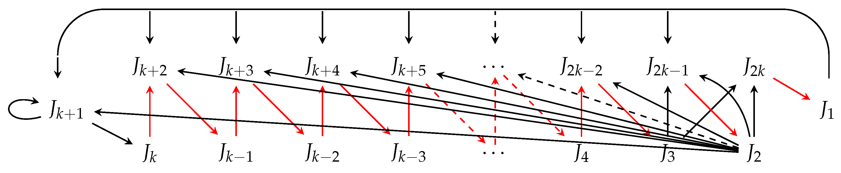
The digraph of a cycle with period $m>2$ contains a subgraph $J_{r_{*}}\to \cdots J_r$ for any $1\le r\le m-1$.

Definition 10. 

A cycle in a digraph is said to be primitive if it does not consist entirely of a cycle of smaller length described several times.

Lemma 2 

(Straffin [2,24]). If f has a periodic point of period $n>1$ and its associated digraph contains a primitive cycle $J_0\to J_1\to \cdots \to J_{m-1}\to J_0$ of length m, then f has a periodic point y of period m such that $f^k\left(y\right)\in J_k,(0\le k<m)$.

Lemma 3 

(Converse Straffin [2]). Let f have a periodic point of period $n>1$ with a digraph $\mathbb{D}$. Suppose f is strictly monotonic on each subinterval $J_i=\left[{\beta }_i{\beta }_{i+1}\right]$ for $1\le i\le n-1$. If f has an orbit of period m in the open interval $({\beta }_1,{\beta }_n)$, then either $\mathbb{D}$ contains a primitive cycle of length m or m is even and $\mathbb{D}$ contains a primitive cycle of length $m/2$.

4. Proofs of Theorems 3 and 4

Let $f:I\to I$ be a continuous endomorphism that has a $2k+1$-orbit ($k\ge 4$) that is second minimal. Let $B=\left\{{\beta }_1<{\beta }_2<\cdots <{\beta }_{2k+1}\right\}$ be the ordered elements of this orbit; and let $r_{*}=max\left\{i\mid f\left({\beta }_i\right)>{\beta }_i\right\}$. Such an $r_{*}$ exists since $f\left({\beta }_1\right)>{\beta }_1$ and $f\left({\beta }_{2k+1}\right)<{\beta }_{2k+1}$. So, $J_{r_{*}}\to J_{r_{*}}$; Let $B^{-}=\left\{\beta \in B\mid \beta \le {\beta }_{r_{*}}\right\},B^{+}=\left\{\beta \in B\mid \beta >{\beta }_{r_{*}}\right\}$; thus, we have $\left|B^{-}\right|+\left|B^{+}\right|=2k+1$ and hence, $\left|B^{-}\right|\ne \left|B^{+}\right|$. Assume, without loss of generality, $\left|B^{-}\right|>\left|B^{+}\right|$. Let $r=max\left\{i<r_{*}\mid f\left({\beta }_i\right)\le {\beta }_{r_{*}}\right\}$. We have $f\left({\beta }_r\right)\le {\beta }_{r_{*}}$, $f\left({\beta }_{r+1}\right)>{\beta }_{r_{*}}$ and hence, $J_r\to J_{r_{*}}$. From Lemma 1, the existence of the subgraph

$$\circlearrowleft J_{r_{*}}\to \cdots \to J_r\to J_{r_{*}}$$

(6)

follows. Assume that (6) presents the shortest path. Since there are $2k$ intervals, its length is at most $2k+1$ and at least $2k-1$. Indeed, if its length is $2k-2$ or less, then Lemma 2 implies the existence of an odd periodic orbit of period $2k-3$ or less. Let us change the indices of intervals in (6) successively as $r_{*}=r_1,\cdots ,r=r_m$ and write path (6) as

$$\circlearrowleft J_{r_1}\to \cdots \to J_{r_m}\to J_{r_1}$$

(7)

where $m=2k-2$, $2k-1$, or $2k$; for simplicity, we are going to use the notation i for ${\beta }_i$. In the sequel, the notation $\begin{array}{c}a\\ b\end{array}$ in the second row of the cyclic permutation means that either of the entries a or b is a valid choice for the image of the node in the same column of the first row; $J_{r_i}\to [a,b]$ means $f\left(r_i\right)=a$ and $f(r_i+1)=b$, the notation $\langle J_r,J_s\rangle$ means the union of $J_r$, $J_s$ and all the intervals between them. Note that if $J_{r_i}\to J_{r_j}$ and $J_{r_i}\to J_{r_k}$, then $J_{r_i}\to 〈J_{r_j},J_{r_k}〉$.

Since (7) is the shortest path, we have

$$\begin{array}{cc}\hfill J_{r_i}& \cancel{\to }{J}_{r_j}\mathrm{for}j>i+1,1\le i\le m-2;\hfill \end{array}$$

(8a)

$$\begin{array}{cc}\hfill J_{r_i}& \cancel{\to }{J}_{r_1}\mathrm{for}2\le i\le m-1;\hfill \end{array}$$

(8b)

we also have

$$J_{r_i}\cancel{\to }{J}_{r_j}\mathrm{for}1<j<i,4\le i\le m,i-j\mathrm{even};$$

(9)

unless $i=m=2k$, $j=2$. Indeed, otherwise according to Lemma 2, an odd orbit of length less than $2k-1$ must exist. From (8) and (9), we can infer the relative position of the intervals to be either (Figure 2)

Or (Figure 3).

If $m=2k$, then the path (7) contains all $2k$ intervals. From the proof of Theorem 2 (for example, see Proposition 8 in [2]), it follows that the corresponding periodic orbit is a Stefan orbit.

Lemma 4. 

The case when $m=2k-1$ produces exactly 2 second minimal $(2k+1)$-orbits. Cyclic permutations are given in (10) and (11), and the corresponding digraphs are presented in Figure 4 and Figure 5, respectively.

$$\left(\begin{array}{ccccccccc}1& 2& \cdots & k-2& k-1& k& k+1& k+2& \cdots \\ k+1& 2k+1& \cdots & k+5& k+2& k+4& k+3& k& \cdots \end{array}\right)$$

(10)

$$\left(\begin{array}{cccccccccc}1& 2& \cdots & k-2& k-1& k& k+1& k+2& k+3& \cdots \\ k& 2k+1& \cdots & k+5& k+4& k+2& k+3& k+1& k-1& \cdots \end{array}\right)$$

(11)

Proof. 

When the length of the path (7) is $2k-1$, we have exactly one interval, call it $\tilde{J}$, missing. Since $J_{r_{2k-1}}\to J_{r_1}$, $J_{r_{2k-1}}\cancel{\to }{J}_{r_i}$ for $i>1$ odd, one of the endpoints of $J_{r_{2k-1}}$ must be mapped to some element of the orbit that separates $J_{r_1}$ and $J_{r_3}$. Since $\circlearrowleft J_{r_1}\to J_{r_2}$, but $J_{r_1}\cancel{\to }{J}_{r_3}$, it follows that the endpoint of $J_{r_1}$ that separates $J_{r_1}$ and $J_{r_2}$ must be mapped to the element of the orbit that separates $J_{r_1}$ and $J_{r_3}$. Therefore, unless there is an interval between $J_{r_1}$ and $J_{r_3}$, the element of the orbit that separates $J_{r_1}$ and $J_{r_3}$ will be an image of two distinct elements of the orbit. Hence, $\tilde{J}$ is between $J_{r_1}$ and $J_{r_3}$, and the distribution of the intervals is as in Figure 6 or Figure 6 reflected about the center point $k+1$. Note that the distribution described in Figure 6 is relevant due to our assumption $\left|B^{-}\right|>\left|B^{+}\right|$. The other case will provide the associated inverse digraph with $\left|B^{+}\right|>\left|B^{-}\right|$. Hence, the structure is as described in Figure 6.

This implies the following cyclic permutation. Note the possible alternation of images of elements 1, $k+2$, $k-1$, and k.

$$\left(\begin{array}{ccccccccc}1& \cdots & k-1& k& k+1& k+2& k+3& k+4& \cdots \\ \begin{array}{c}k+1\\ k\end{array}& \cdots & \langle k+2,& k+4\rangle & k+3& \begin{array}{c}k\\ k+1\end{array}& k-1& k-2& \cdots \end{array}\right)$$

(12)

• Case $\left(1\right)$: $f(k-1)=k+2\Rightarrow f\left(k\right)=k+4$
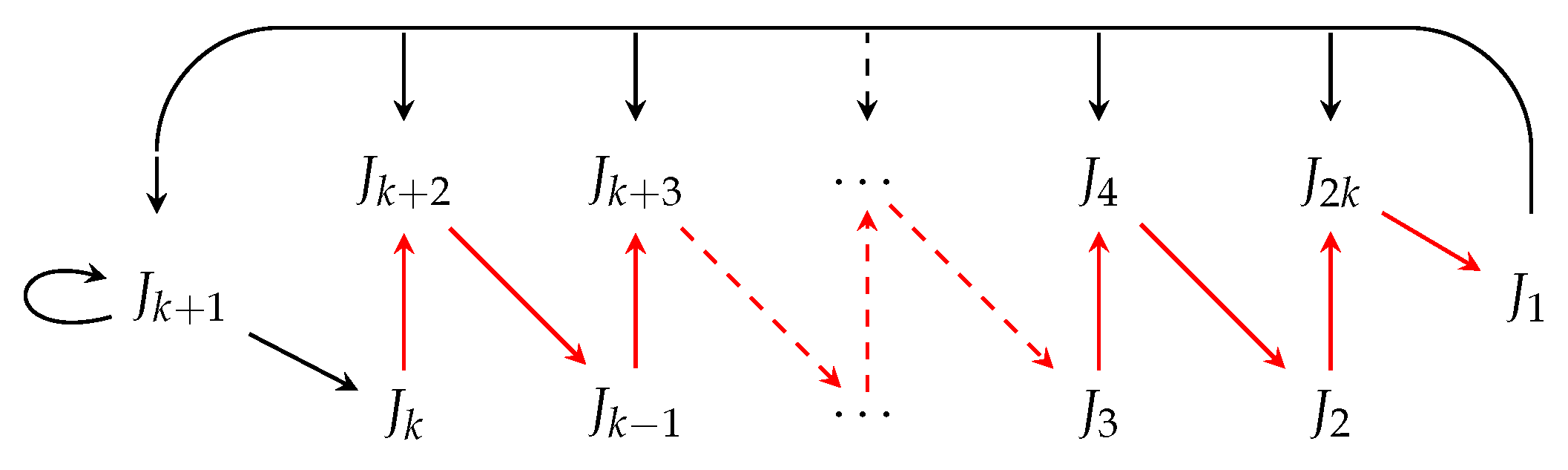
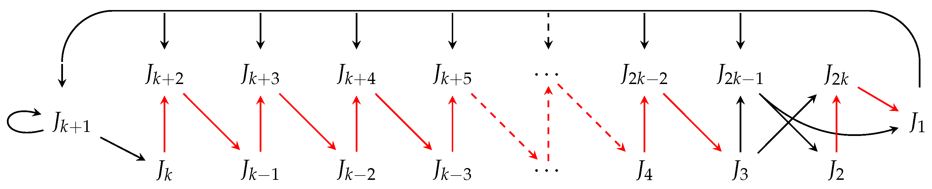
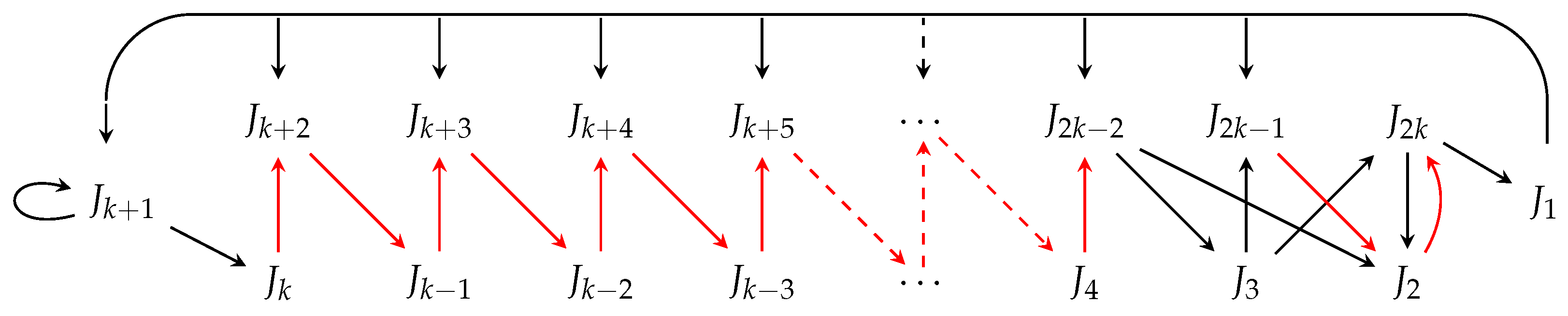
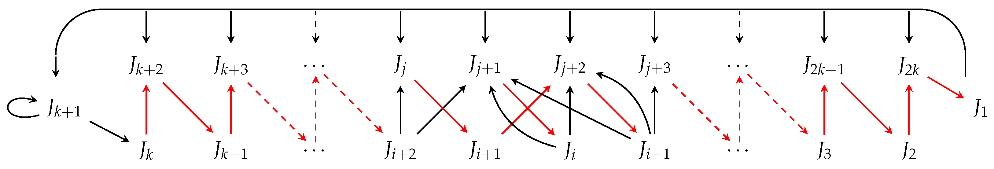
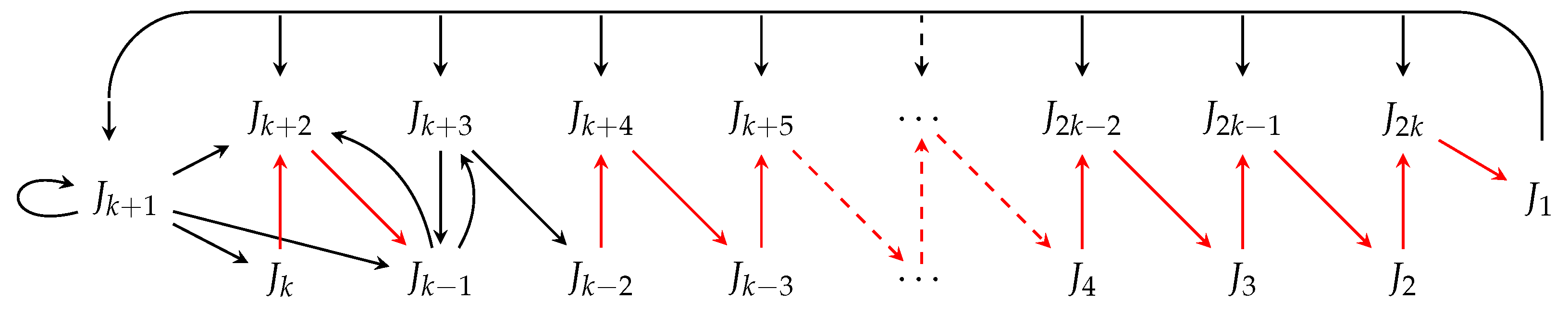
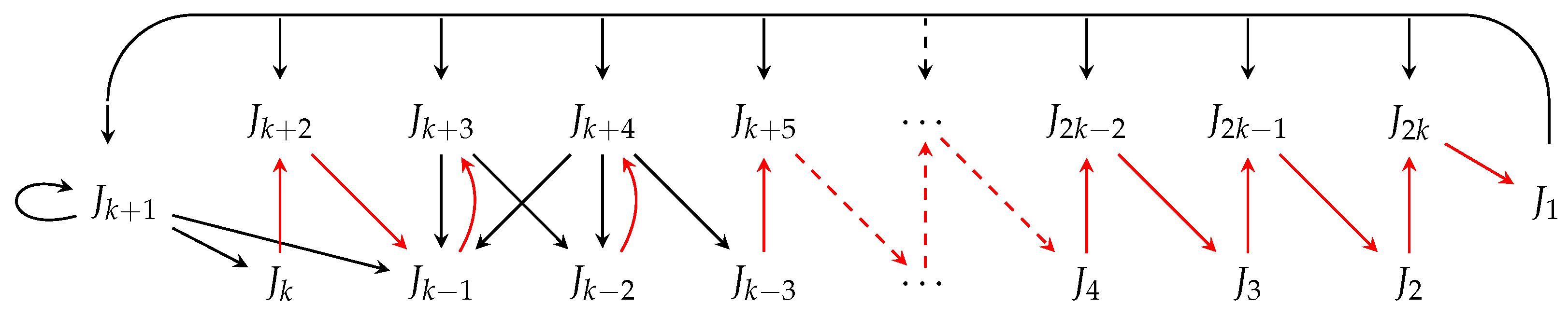
• Case ${\left(1\right)}_1$: $f\left(1\right)=k+1\Rightarrow f(k+2)=k$; This produces a simple positive type $(2k+1)$-orbit given in (10) and Figure 4 with topological structure max-min-max. Next, we analyze the digraph to show that there are no primitive cycles of even length $\le 2k-2$, which would imply by Straffin’s lemma, an existence of odd periodic orbit of length $\le 2k-3$. From Lemma 3, it then follows that the P-linearization of the orbit (10) presents an example of a continuous map with a second minimal $(2k+1)$-orbit. We split the analysis into two cases:

  (a)

  Consider primitive cycles that contain $J_1$. Without any loss of generality, choose $J_1$ as the starting vertex. First, assume that the cycle does not start with chain $J_1\to J_{k+1}$. Since $J_{2k+1-i}\to J_i,i=1,\dots ,k-1,$ any such cycle can be formed only by adding on to the starting vertex $J_1$ pairs $(J_{2k+1-i},J_i),i=1,\dots ,k-1$. Therefore, the length of the cycle (by counting $J_1$ twice) will always be an odd number. Conversely, if the cycle starts with chain $J_1\to J_{k+1}$, then to close it at $J_1$, the smallest required even length is $2k$.

  (b)

  Consider primitive cycles that do not contain $J_1$. Obviously, such a cycle does not contain $J_2,J_3,\dots ,J_{k-3}$ or $J_{k+4},J_{k+5},\dots ,J_{2k-1},J_{2k}$ since these vertices have red edges connecting them all the way to $J_1$. Additionally, this cycle cannot contain $J_{k+1}$ or $J_k$ since $J_1$ is the only vertex (besides $J_{k+1}$ itself) with a directed edge to $J_{k+1}$, and $J_{k+1}$ is the only vertex with a directed edge to $J_k$. This leaves 4 vertices: $J_{k-2},J_{k-1},J_{k+2},J_{k+3}$. Since $J_{k+2}\to J_{k-1}$, $J_{k+3}\to J_{k-2}$ and $J_{k+2}\leftrightharpoons J_{k-1}$, $J_{k+3}\leftrightharpoons J_{k-2}$, any cycle formed by these four vertices will consist of a starting vertex followed (or ending vertex preceded) by pairs $(J_{k+2},J_{k-1})$, $(J_{k+3},J_{k-2})$ added arbitrarily many times, and hence no cycles of even length can be produced.

• Case ${\left(1\right)}_2$: $f\left(1\right)=k\Rightarrow f(k+2)=k+1$, then we have the period 4-suborbit
  $\left\{k-1,k+1,k+2,k+3\right\}$, a contradiction.
• Case $\left(2\right)$: $f(k-1)=k+4\Rightarrow f\left(k\right)=k+2$.
• Case ${\left(2\right)}_1$: $f\left(1\right)=k+1\Rightarrow f(k+2)=k$, then we have the period 2-suborbit $\left\{k,k+2\right\}$, a contradiction.
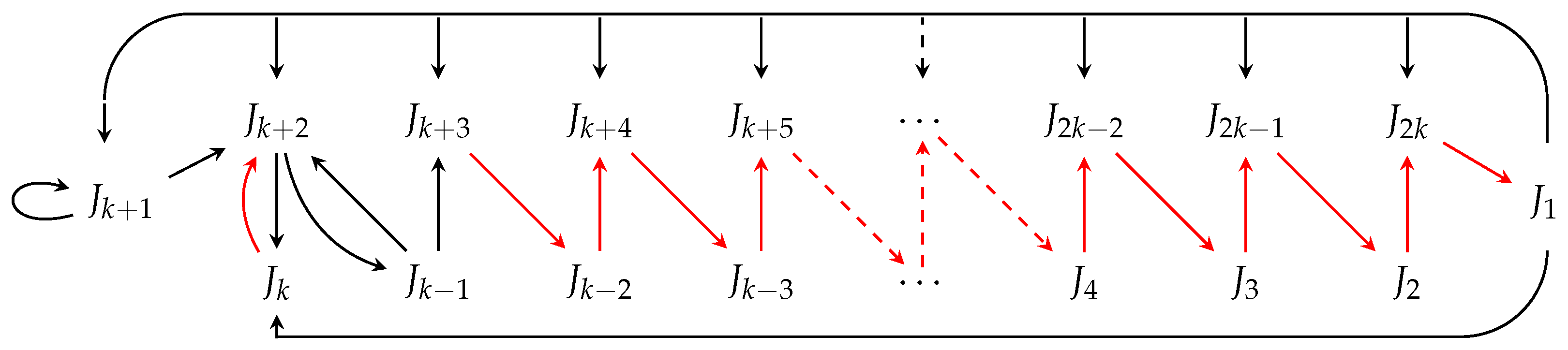
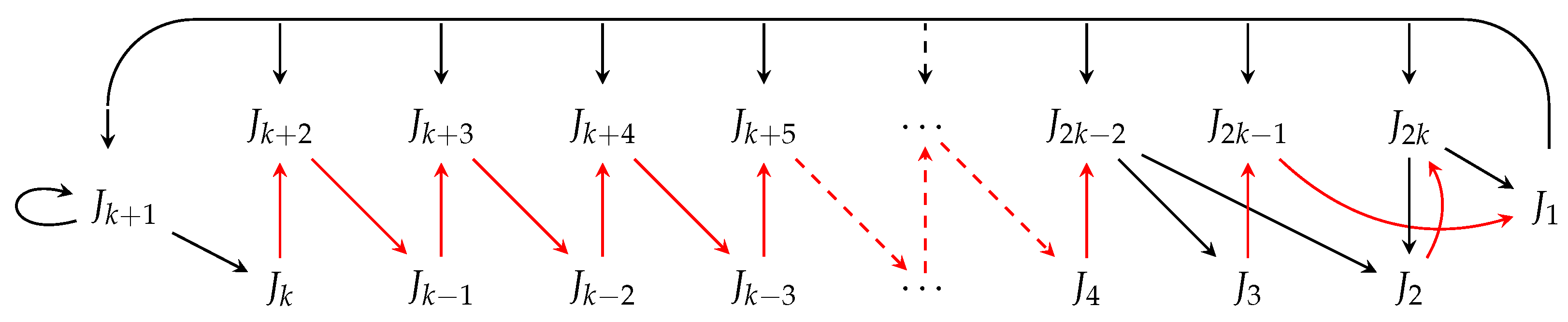
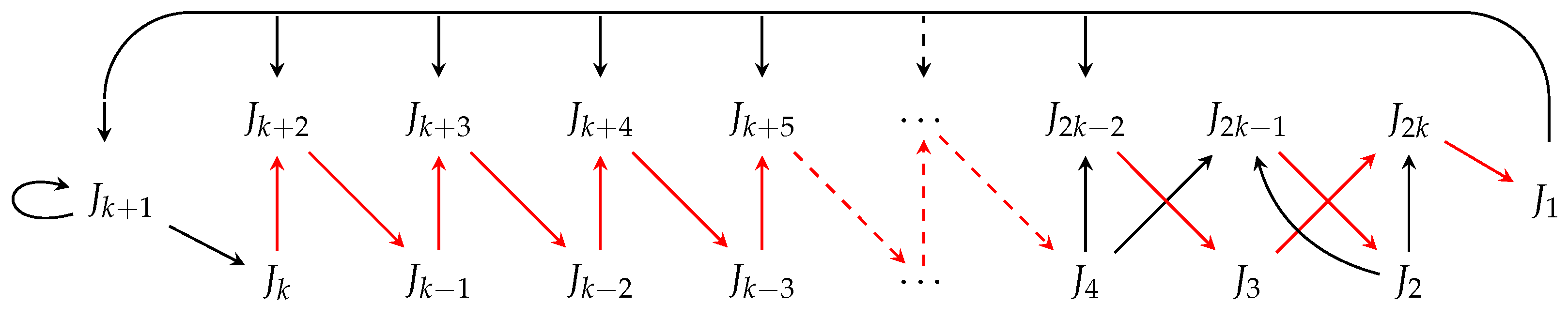
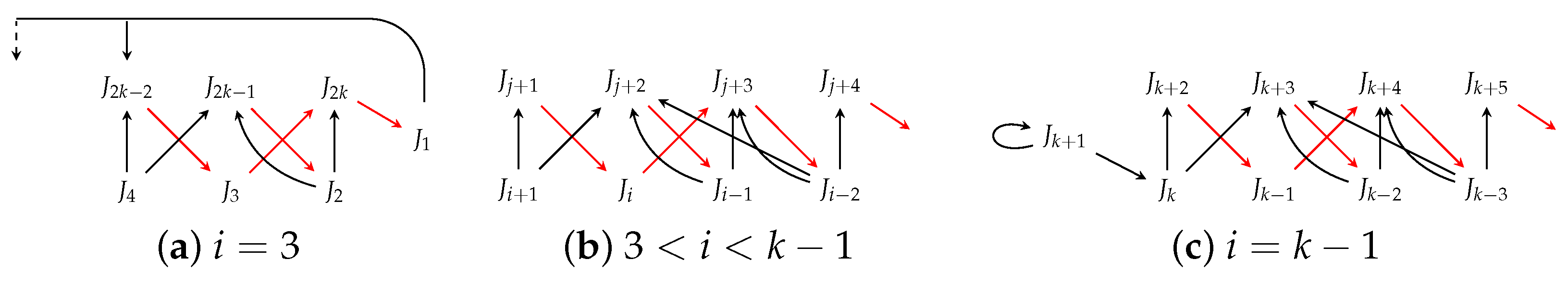
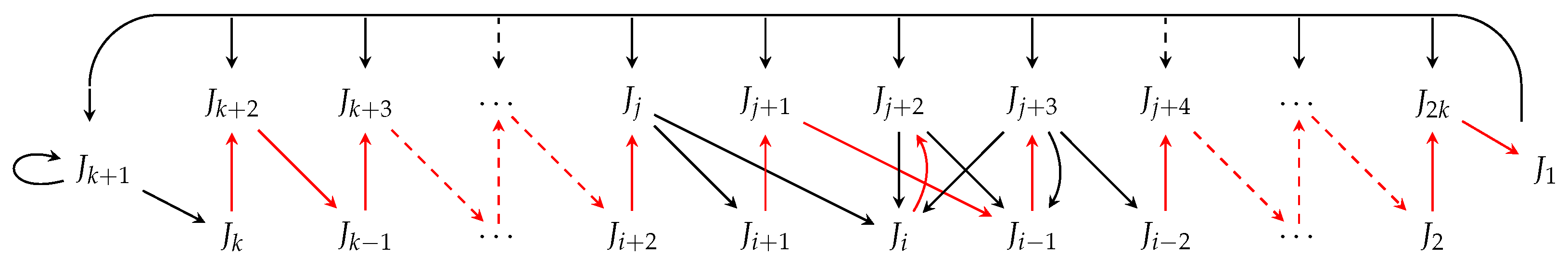
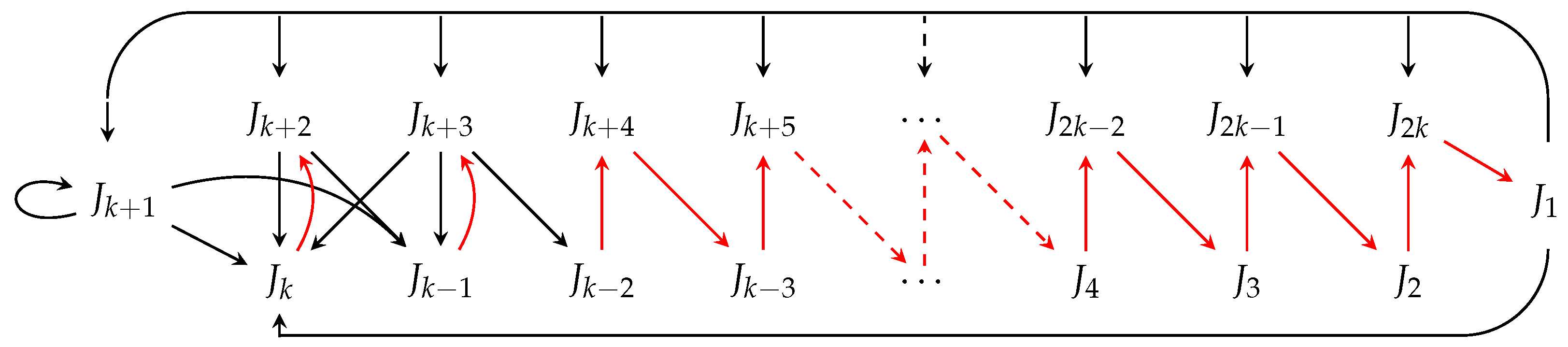
• Case ${\left(2\right)}_2$: $f\left(1\right)=k\Rightarrow f(k+2)=k+1$; This produces a simple positive type $(2k+1)$-orbit given in (11) and Figure 5 with topological structure max-min-max. We repeat the argument from Case ${\left(1\right)}_1$. First, we analyze the digraph to show that there are no primitive cycles of even length $\le 2k-2$. We split the analysis into two cases:

  (a)

  Consider primitive cycles that contain $J_1$. Without any loss of generality, choose $J_1$ as a starting vertex. First, assume that the cycle starts with the edge $J_1\to J_j$, with j taking any value between $k+3$ and $2k$. Since $J_{2k+1-i}\to J_i,i=1,\dots ,k-2,$ any such cycle can be formed only by adding to starting vertex $J_1$ pairs $(J_{2k+1-i},J_i),i=1,\dots ,k-2$. Therefore, the length of the cycle (by counting $J_1$ twice) will be always an odd number. If the cycle starts with the edge $J_1\to J_{k+2}$, then the only difference from the previous case will be the addition of the pairs $(J_{k+2},J_{k-1})$ and/or $(J_{k+2},J_k)$ arbitrarily many times. Hence, only cycles of odd length will be produced. Conversely, if the cycle starts with the chain $J_1\to J_{k+1}$ or $J_1\to J_k$, then to close it at $J_1$, the smallest required even length is $2k$.

  (b)

  Consider a primitive cycle that does not contain $J_1$. Obviously, such a cycle does not contain $J_2,J_3,\dots ,J_{k-2}$ or $J_{k+3},J_{k+4},\dots ,J_{2k-1},J_{2k}$ since these vertices have red edges connecting them all the way to $J_1$. Additionally, this cycle cannot contain $J_{k+1}$ since $J_1$ is the only vertex (besides $J_{k+1}$ itself) with a directed edge to $J_{k+1}$. This leaves 3 vertices: $J_k,J_{k-1},J_{k+2}$ connected as $J_k\leftrightharpoons J_{k+2}\leftrightharpoons J_{k-1}$. Therefore, this triple can only produce cycles when pairs $(J_{k+2},J_{k-1})$ and $(J_{k+2},J_k)$ are added to a starting vertex. Therefore, no cycle of even length can be produced.

□

Now, observe that when the length, m, of path (7) is $2k-2$, it is comprised of $2k-2$ distinct intervals and thus there are 2 additional intervals required to complete the periodic orbit of period $2k+1$. From path (7) and the rules (8), it follows that the relative distribution of the $2k-2$ intervals is in one of the following 2 forms illustrated in Figure 7 and Figure 8. Call the two missing intervals $\tilde{J}$ and $\widehat{J}$. There are $2k-1$ slots in Figure 7 and Figure 8 where we can place each of these extra intervals for a total of ${(2k-1)}^2$ pairs. However, since swapping the locations of $\tilde{J}$ and $\widehat{J}$ does not affect the analysis, let us consider the distribution given in Figure 8 in the upper triangular matrix (13), where $(i,j)$ indicates placing $\tilde{J}$ in position i and $\widehat{J}$ in position j.

$$\begin{array}{ccccccc}(1,1)& (1,2)& (1,3)& \cdots & (1,2k-3)& (1,2k-2)& (1,2k-1)\\ & (2,2)& (2,3)& \cdots & (2,2k-3)& (2,2k-2)& (2,2k-1)\\ & & (3,3)& \cdots & ⋮& & ⋮\\ & & & \ddots & (i,i)& \cdots & (i,2k-i+2)\\ & & & & \ddots & ⋮& ⋮\\ & & & & & \ddots & (2k-1,2k-1)\end{array}$$

(13)

The next lemma specifies all the entries $(i,j)$ in matrix (13) such that insertion of $(\tilde{J},\widehat{J})$ in $(i,j)$ can produce second minimal odd orbits.

Lemma 5. 

Fix the entry point, i, for $\tilde{J}$, then, to produce second minimal $2k+1$ orbit, $\widehat{J}$ can only be placed in

1. 

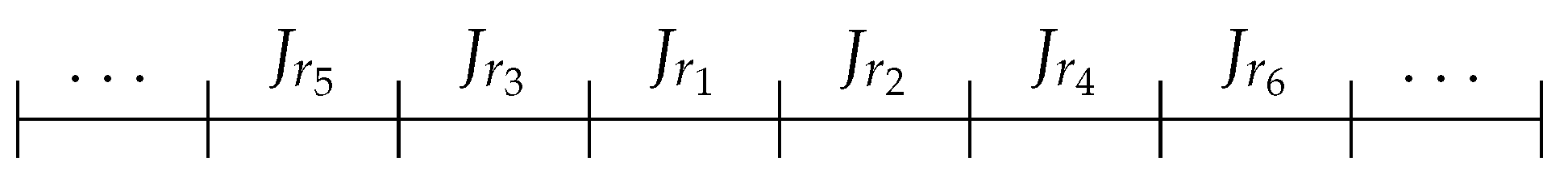
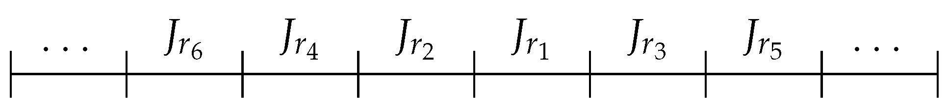
position $2k-1$ when $i=1$,

2. 

positions $2k-i$ or $2k-i+1$ for $1<i<k$,

3. 

and position $k+1$ when $i=k$.

Proof. 

Let $1<i<k$ for $k>3$. Let the interval immediately to the left of $\tilde{J}$ be called $J_{r_w}$, or the w-th distinct interval in path (7). From the relative positions of the intervals in Figure 3, it is clear that $w=2(k-i+1)$. As depicted in Figure 9, the intervals to the right of $\tilde{J}$ have a set path. $J_{r_{w-4}}$ maps only to $J_{r_{w-3}}$, $J_{r_{w-2}}$ maps only to $J_{r_{w-1}}$, etc. Note that while the exact points that these intervals map to might change upon the insertion of $\widehat{J}$, the overall structure must remain the same in order to preserve path (7).

However, this pattern can no longer be continued indefinitely for interval $J_{r_w}$. $J_{r_w}$ must be mapped to $J_{r_{w+1}}$, by definition. This implies that one end point of $J_{r_w}$ is mapped arbitrarily to the left of $J_{r_{w+1}}$ and the other endpoint is mapped arbitrarily to the right of $J_{r_{w+1}}$. According to (8), $J_{r_w}$ cannot map to any odd interval greater than $J_{r_{w+1}}$. Assuming that $J_{r_{w+1}}$ is not the rightmost interval, or in other words $w+1<2k-3$, then the endpoint of $J_{r_w}$ that maps to the right of $J_{r_{w+1}}$ must map to a point separating $J_{r_{w+1}}$ and $J_{r_{w+3}}$. This could either be a point directly in between $J_{r_{w+1}}$ and $J_{r_{w+3}}$ or a new point between $J_{r_{w+1}}$ and $J_{r_{w+3}}$, upon the insertion of $\widehat{J}$.

Note that if $w+1=2k-3$, or in other words $J_{r_{w+1}}$ is the rightmost interval, then $J_{r_{w+3}}$ no longer exists. Rather than mapping to a point separating $J_{r_{w+1}}$ and $J_{r_{w+3}}$, an endpoint of $J_{r_w}$ will just map to the right of $J_{r_{w+1}}$.

While it is clear how one endpoint of $J_{r_w}$ will map to the right of $J_{r_{w+1}}$, it is much less clear how an endpoint of $J_{r_w}$ will map to the left of $J_{r_{w+1}}$. According to (9), $J_{r_w}$ cannot map to $J_{r_1}$ or any $J_{r_k}$ where $k<w$ and is even. Thus, the arbitrary point to the left of $J_{r_{w+1}}$ to which an endpoint of $J_{r_w}$ must map must be separating $J_{r_1}$ and $J_{r_{w+1}}$. Thus, the missing interval $\widehat{J}$ must be inserted between $J_{r_1}$ and $J_{r_{w+1}}$. Note that according to the previously mentioned positional notation, this includes all the positions $k+1$, $k+2$, …, $2k-i$, $2k-i+1$.

Suppose that the interval $\widehat{J}$ is inserted into a position to the left of $2k-i$. Assume, without any loss of generality, that the interval $\widehat{J}$ is inserted into position $2k-i-1$ (between intervals $J_{r_{w-3}}$ and $J_{r_{w-5}}$ if $w\ge 6$, and between $J_{r_1}$ and $J_{r_2}$ if $w=4$), as the contradiction will be the same. The interval immediately to the right of $\widehat{J}$ has some trouble mapping to the interval indexed one greater than itself. In the situation where $\widehat{J}$ is placed in position $2k-i-1$, the interval immediately to the right of $\widehat{J}$ is $J_{r_{w-3}}$, which has trouble mapping to $J_{r_{w-2}}$. One endpoint of $J_{r_{w-3}}$ must map to the left of $J_{r_{w-2}}$, while the other must map to the right of $J_{r_{w-2}}$. Again, according to (9), $J_{r_{w-3}}$ cannot map to a lesser odd interval or $J_{r_1}$. Thus, the only available point to the left of $J_{r_1}$ and to the right of $J_{r_{w-2}}$ is the point indexed $k+1$ or the left endpoint of $J_{r_1}$. However, it is important to note that the largest indexed interval, $J_{r_{2k-2}}$, must also map back to $J_{r_1}$. Furthermore, according to (9), $J_{r_{2k-2}}$ cannot map to a lesser even interval, specifically including $J_{r_2}$. Therefore, an endpoint of $J_{r_{2k-2}}$ must map to the left of $J_{r_1}$, but cannot map to the left of $J_{r_2}$. The only point that fits this description is the one indexed $k+1$. Thus, the point $k+1$ is already taken, and an endpoint of $J_{r_{w-3}}$ cannot map to the point indexed $k+1$. Furthermore, there are no open points that are both to the right of $J_{r_{w-2}}$ and to the left of $J_{r_1}$. This is an immediate contradiction, as it is now impossible for an endpoint of $J_{r_{w-3}}$ to map to the right of $J_{r_{w-2}}$, making it impossible for $J_{r_{w-3}}$ to contain $J_{r_{w-2}}$.

Now, suppose instead that $w=4$. If this is the case, then $\widehat{J}$ is inserted between $J_{r_1}$ and $J_{r_2}$. Again, the image of $J_{r_1}$ must contain only $J_{r_1}$ and $J_{r_2}$. Thus, one endpoint of $J_{r_1}$ must map to the right of $J_{r_1}$, but cannot map to the right of $J_{r_3}$. Therefore, the left endpoint of $J_{r_1}$ must map to the point separating $J_{r_1}$ and $J_{r_3}$. Now, $J_{r_2}$ must map to $J_{r_3}$, but cannot map back to $J_{r_1}$. Thus, one of the endpoints of $J_{r_2}$ must map to a point separating $J_{r_1}$ and $J_{r_3}$. Both the left endpoint of of $J_{r_1}$ and an endpoint of $J_{r_2}$ must map to points separating $J_{r_1}$ and $J_{r_3}$. There is only one point separating $J_{r_1}$ and $J_{r_3}$, so this is an immediate contradiction.

Therefore, it is impossible for $\widehat{J}$ to be inserted to the left of position $2k-i$, because the interval immediately to the right of $\widehat{J}$ can no longer map to the interval indexed one greater than itself, in the case of $w\ge 6$. In the case of $w=4$, a separate contradiction arises when both the left endpoint of of $J_{r_1}$ and an endpoint of $J_{r_2}$ must map to the singular point separating $J_{r_1}$ and $J_{r_3}$. The only two possible positions of $\widehat{J}$ that can produce valid second minimal orbits when $\tilde{J}$ is inserted into position i, are the positions $2k-i$ and $2k-i+1$.

Suppose that $\tilde{J}$ is inserted into position k. By (8), the image of $J_{r_1}$ must contain itself. This means, by definition, that one endpoint of $J_{r_1}$ must map to the right of itself and the other endpoint of $J_{r_1}$ must map to the left of itself. However, by (8), $J_{r_1}$ cannot map to $J_{r_3}$. Thus, the endpoint of $J_{r_1}$ that maps to the right of itself must map to the left of $J_{r_3}$. In other words, one endpoint of $J_{r_1}$ must map to a point separating $J_{r_1}$ and $J_{r_3}$. By (8), the image of $J_{r_2}$ must contain $J_{r_3}$. Again, this means that one endpoint of $J_{r_2}$ maps to the left of $J_{r_3}$ and the other endpoint of $J_{r_2}$ maps to the right of $J_{r_3}$. However, by (9), the image of $J_{r_2}$ cannot contain $J_{r_1}$. Thus, the endpoint of $J_{r_2}$ that maps to the left of $J_{r_3}$ cannot map to the left of $J_{r_1}$. In other words, an endpoint of $J_{r_2}$ must map to points separating $J_{r_1}$ and $J_{r_3}$. Both an endpoint of $J_{r_1}$ and an endpoint $J_{r_2}$ must map to points separating $J_{r_1}$ and $J_{r_3}$. Note that, when $\tilde{J}$ was inserted into position k, $J_{r_1}$ and $J_{r_2}$ no longer shared an endpoint. Thus, the two endpoints that map to points separating $J_{r_1}$ and $J_{r_3}$ must necessarily be two different points. Thus, there must be at least two different points separating $J_{r_1}$ and $J_{r_3}$. This can only be achieved by inserting $\widehat{J}$ between $J_{r_1}$ and $J_{r_3}$, which is position $k+1$. Or in other words, if $\tilde{J}$ is inserted into position k, a valid second minimal orbit can only be constructed if $\widehat{J}$ is inserted into position $k+1$.

Finally, suppose that $\tilde{J}$ is inserted into position 1. There are two options here:

• $\widehat{J}$ is inserted arbitrarily to the left of $J_{r_1}$.
• $\widehat{J}$ is inserted arbitrarily to the right of $J_{r_1}$.

Suppose that $\widehat{J}$ is inserted arbitrarily to the left of $J_{r_1}$. If $\widehat{J}$ is in any position j, where $2\le j\le k$. By simply changing the notation, where $\widehat{J}$ becomes $\tilde{J}$ and $\tilde{J}$ becomes $\widehat{J}$, we suddenly have the cases already addressed earlier in the proof, with $\tilde{J}$ being arbitrarily between $J_{r_{2k-2}}$ and $J_{r_1}$. Note that for none of the cases where $2\le i\le k$, position 1 was not a valid position for $\widehat{J}$. Thus, the only case that has not been considered is when both $\tilde{J}$ and $\widehat{J}$ are in position 1. For the sake of simplicity, assume that $\widehat{J}$ is the first interval, and $\tilde{J}$ is the interval between $\widehat{J}$ and $J_{r_{2k-2}}$.

It follows from (8) that the image of $J_{r_1}$ must contain only itself and $J_{r_2}$. This is only possible if the left endpoint of $J_{r_1}$, indexed $k+2$, maps to the right endpoint of $J_{r_1}$, which is indexed $k+3$; and the right endpoint of $J_{r_1}$ maps to the left endpoint of $J_{r_2}$, indexed $k+1$. By (8), $J_{r_2}$ must contain $J_{r_3}$ and no odd interval with a greater index, which is only possible if the left endpoint of $J_{r_2}$, indexed k, maps to the right endpoint of $J_{r_3}$, indexed $k+4$. Furthermore, by (8), every even interval can contain only the odd interval indexed one greater than itself and no greater odd interval, and conversely, every odd interval can contain only the even interval indexed one greater than itself and no greater even interval. This fact forces the intervals to follow the structure depicted in [6]. This pattern continues until the left endpoint of $J_{r_{2k-3}}$ maps to the right endpoint of $J_{r_{2k-2}}$ and the left endpoint of $J_{r_{2k-4}}$ maps to the right of $J_{r_{2k-3}}$. This construction yields Figure 10, where the solid red lines represent the Stefan-like structure present when $\tilde{J}$ and $\widehat{J}$ are both placed in Position 1.

By (8), the image of $J_{r_{2k-2}}$ must contain $J_{r_1}$, but cannot map to a lesser even interval, specifically $J_{r_2}$. Therefore, the left endpoint of $J_{r_{2k-2}}$ must map somewhere to the left of $J_{r_1}$ but cannot map to the left of $J_{r_2}$. In other words, it must map to a point separating $J_{r_1}$ and $J_{r_2}$. The only point that meets this condition is indexed $k+2$. Therefore, the left endpoint of $J_{r_{2k-2}}$ must map to the point indexed $k+2$, shown by the dotted red line in Figure 10.

By (8), the image of $J_{r_{2k-3}}$ must contain $J_{r_{2k-2}}$. Thus, the right endpoint of $J_{r_{2k-3}}$ must map to the left of $J_{r_{2k-2}}$. However, note if the right endpoint of $J_{r_{2k-3}}$ maps immediately to the left of $J_{r_{2k-2}}$ to the point indexed 3, then two closed sub-orbits of length 2 and of the form $\left\{1,2\right\}$ are formed. Thus, the right endpoint of $J_{r_{2k-3}}$ can map either to the point indexed 1 or the point indexed 2. Investigating both of these cases individually leads to quick contradictions.

Suppose that the right endpoint of $J_{r_{2k-3}}$ maps to the left endpoint of $\widehat{J}$ or the point indexed 1. The only two ‘open’ points, or points that do not already have a point mapping to them, are the ones indexed 2 and 3. Because point 2 cannot map to itself, it must map to the only other open point, indexed 3. The final point, indexed 1, can now only map to point 2, completing the cyclic permutation. However, this can instantly be shown to be an invalid cyclic permutation due to the presence of a 3 orbit of the form $\tilde{J}\to J_{r_{2k-2}}\to J_{r_{2k-3}}\to \tilde{J}$.

Since the left endpoint of $J_{r_{2k-3}}$ cannot map to the point indexed 1, the case where the left endpoint of $J_{r_{2k-3}}$ maps to the point indexed 2 is considered. Now, the only two open points are the ones indexed 1 and 3. Because point 1 cannot map to itself, it must map to the only other open point, indexed 3. The final point, indexed 2, can now only map to point 1, completing the cyclic permutation. However, this can instantly be shown to be an invalid cyclic permutation due to the presence of a 3 orbit of the form $\widehat{J}\to \tilde{J}\to \widehat{J}\to \widehat{J}$.

This exhausts all possible options for points that the right endpoint of $J_{r_{2k-3}}$ can map to, proving that it is impossible to form a valid cyclic permutation when $\tilde{J}$ and $\widehat{J}$ are both in position 1. Furthermore, all cases where $\tilde{J}$ is in position 1 and $\widehat{J}$ is in an arbitrary position j, where $2\le j\le k$ have been proven to lead to contradictions. Thus, any case where $\tilde{J}$ is in position 1 and $\widehat{J}$ is inserted arbitrarily to the left of $J_{r_1}$ cannot lead to the construction of a valid second minimal odd orbit.

A valid second minimal odd orbit for the case where $\tilde{J}$ is in position 1 can only be constructed when $\widehat{J}$ is inserted arbitrarily to the right of $J_{r_1}$. Consider the case when $\widehat{J}$ is inserted between $J_{r_1}$ and $J_{r_{2k-3}}$. Now, assume without any loss of generality that $\widehat{J}$ is inserted to the position immediately to the left of $J_{r_{2k-3}}$, as the contradiction will be the same. The interval immediately to the right of $\widehat{J}$, in this case $J_{r_{2k-3}}$, has trouble mapping to the interval indexed one greater than itself, in this case $J_{r_{2k-2}}$. While it is clear how an endpoint of $J_{r_{2k-3}}$ will map to the left of $J_{r_{2k-2}}$, it is much less clear how an endpoint will map to the right of $J_{r_{2k-3}}$. Again, according to (9), the image of $J_{r_{2k-3}}$ cannot contain $J_{r_1}$. Thus, an endpoint of $J_{r_{2k-3}}$ must map to a point separating $J_{r_{2k-2}}$ and $J_{r_1}$. The only point that fits this description is the one indexed $k+1$. However, it is important to note that the largest indexed interval, $J_{r_{2k-2}}$, must also map back to $J_{r_1}$. Furthermore, according to (9), $J_{r_{2k-2}}$ cannot map to a lesser even interval, specifically including $J_{r_2}$. Therefore, an endpoint of $J_{r_{2k-2}}$ must map to the left of $J_{r_1}$ but cannot map to the left of $J_{r_2}$. The only point that fits this description is the one indexed $k+1$, which is already taken. This is an immediate contradiction, as both an endpoint of $J_{r_{2k-3}}$ and an endpoint of $J_{r_{2k-2}}$ must map to the point indexed $k+1$. Therefore, it is impossible for $\widehat{J}$ to be placed between $J_{r_1}$ and $J_{r_{2k-3}}$. The only possible way to make the construction of valid second minimal odd orbits possible when $\tilde{J}$ is placed in position one is by placing $\widehat{J}$ into the position $2k-1$ or immediately to the right of $J_{r_{2k-3}}$.

To complete the proof, we show there are no valid settings $(i,j)$ for $k<i\le 2k-1$, $j\ge i$. Note that (13) only includes $(i,j)$ pairs where $j\ge k$, if $i>k$. Thus, both i and j are to the right of $J_{r_1}$. Assume for the sake of simplicity that the interval closer to $J_{r_1}$ is the one labeled $\tilde{J}$. All intervals between $J_{r_1}$ and $\tilde{J}$ will map according to the minimal structure (2) [2], as described earlier. The Stefan structure comes to an end when the interval immediately to the left of $\tilde{J}$, $J_{r_{2i-2k-1}}$ maps to $J_{r_{2i-2k}}$. Now, the interval to the right of $\tilde{J}$, $J_{r_{2i-2k+1}}$ has trouble mapping to the interval $J_{r_{2i-2k+2}}$. $J_{r_{2i-2k+1}}$ cannot map to $J_{r_1}$ according to the rules (8) and (9), so one of its endpoints must map to a point separating $J_{r_1}$ and $J_{r_{2i-2k+2}}$. The only such point is k. However, as discussed before, k must be mapped to by an endpoint of the interval $J_{r_{2k-2}}$. Thus, there are no open points between $J_{r_1}$ and $J_{r_{2i-2k+2}}$. Note that because $\widehat{J}$ is inserted to the right of $\tilde{J}$, it is impossible for an endpoint of $J_{r_{2i-2k+1}}$ to map to the right of $J_{r_{2i-2k+2}}$. Thus, it is impossible for $J_{r_{2i-2k+1}}$ to contain $J_{r_{2i-2k+2}}$ when both $\tilde{J}$ and $\widehat{J}$ are to the right of $J_{r_1}$, which is a clear contradiction. □

Lemma 6. 

Placing $\tilde{J}$ and $\widehat{J}$ in setting $(1,2k-1)$ produces exactly 2 second minimal orbits. These are given in listings (14) and (15) and the corresponding digraphs are presented in Figure 11 and Figure 12, respectively.

$$\left(\begin{array}{cccccccccc}1& 2& 3& \cdots & k+1& k+2& \cdots & 2k-1& 2k& 2k+1\\ 2k+1& k+1& 2k& \cdots & k+2& k& \cdots & 3& 1& 2\end{array}\right)$$

(14)

$$\left(\begin{array}{cccccccccc}1& 2& 3& 4& \cdots & k+1& k+2& \cdots & 2k& 2k+1\\ 2k& k+1& 2k+1& 2k-1& \cdots & k+2& k& \cdots & 2& 1\end{array}\right)$$

(15)

Proof. 

Having inserted $(\tilde{J},\widehat{J})$ in position $(1,2k-1)$, we have the full interval distribution given in Figure 13. Then, using the path (7) and the rules in (8) and (9), we observe that the images of the elements of the cycle from 4 to $2k-1$ are uniquely defined following a Stefan structure as demonstrated in (16).

$$\left(\begin{array}{ccccccc}4& \cdots & k& k+1& k+2& \cdots & 2k-1\\ 2k-1& \cdots & k+3& k+2& k& \cdots & 3\end{array}\right)$$

(16)

The alteration appears only in images of the elements $1,3,2k,2k+1$. By using the path (7) and the rules in (8) and (9) again, we construct the potential cyclic permutation (17) and analyze which of the available choices lead to valid second minimal odd orbits.

$$\left(\begin{array}{ccccccccc}1& 2& 3& \cdots & k+1& \cdots & 2k-1& 2k& 2k+1\\ \begin{array}{c}2k+1\\ 2k\\ 2\end{array}& k+1& \begin{array}{c}2k\\ 2k+1\end{array}& \cdots & k+2& \cdots & 3& \begin{array}{c}1\\ 2\end{array}& \begin{array}{c}2\\ 1\\ 2k\end{array}\end{array}\right)$$

(17)

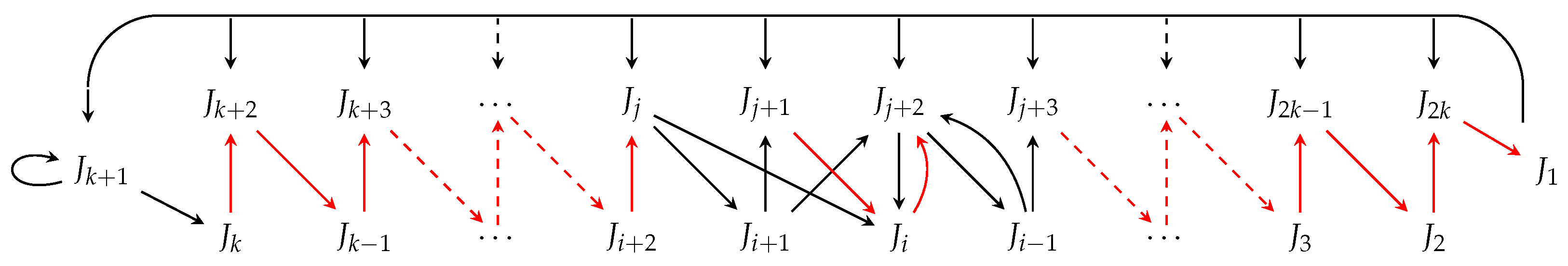
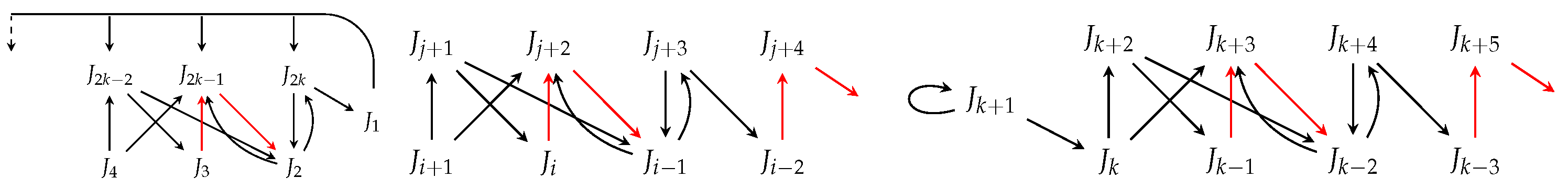
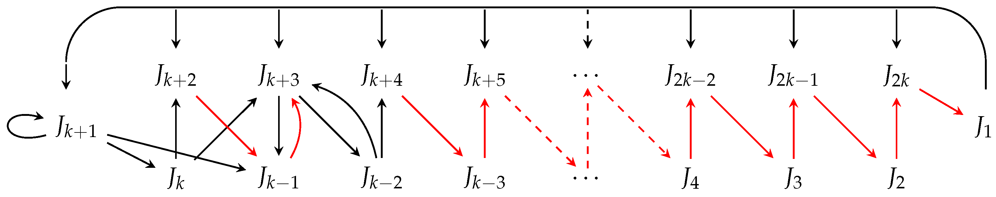
• Case (1): Choosing $f(2k+1)=2\Rightarrow f\left(2k\right)=1,f\left(1\right)=2k+1,f\left(3\right)=2k$; this leads to a valid second minimal orbit with the topological structure min-max-min and the associated digraph is presented in Figure 11 and the cyclic permutation is listed in (14). Next, we analyze the digraph to show that there are no primitive cycles of even length $\le 2k-2$, which would imply by Straffin’s lemma an existence of odd periodic orbit of length $\le 2k-3$. From Lemm 3, it then follows that the P-linearization of the orbit (14) presents an example of a continuous map with a second minimal $(2k+1)$-orbit.

  (a)

  Consider primitive cycles that contain $J_1$. Without any loss of generality, choose $J_1$ as the starting vertex. First, assume that the cycle does not contain $J_{k+1}$. Since $J_{2k+1-i}\to J_i,$$i=1,\dots ,k-1;J_{2k-1}\to J_1$, any such cycle can be formed only by adding to starting vertex $J_1$ pairs $(J_{2k-1},J_1)$, $(J_{2k+1-i},J_i),i=1,\dots ,k-1$. Therefore, the length of the cycle (by counting $J_1$ twice) will be always an odd number. Conversely, if the cycle contains $J_{k+1}$, then to close it at $J_1$, the smallest required even length is $2k+2$.

  (b)

  Consider primitive cycles that do not contain $J_1$, but contain $J_2$. Without any loss of generality, choose $J_2$ as the starting vertex. First, assume that the cycle does not contain $J_{k+1}$. Since $J_{2k+1-i}\to J_i,i=2,\dots ,k-1,$ any such cycle can be formed only by adding to starting vertex $J_2$ pairs $(J_{2k+1-i},J_i),i=2,\dots ,k-1$. Therefore, the length of the cycle (by counting $J_2$ twice) will always be an odd number. Conversely, if the cycle contains $J_{k+1}$, then to close it at $J_2$, the smallest required even length is $2k$. Finally, it is easy to see that by excluding $J_1$ and $J_2$ from the cycle, due to the red edges, all the vertices but $J_{k+1}$ must also be excluded, and cycle at $J_{k+1}$ is the only possibility.

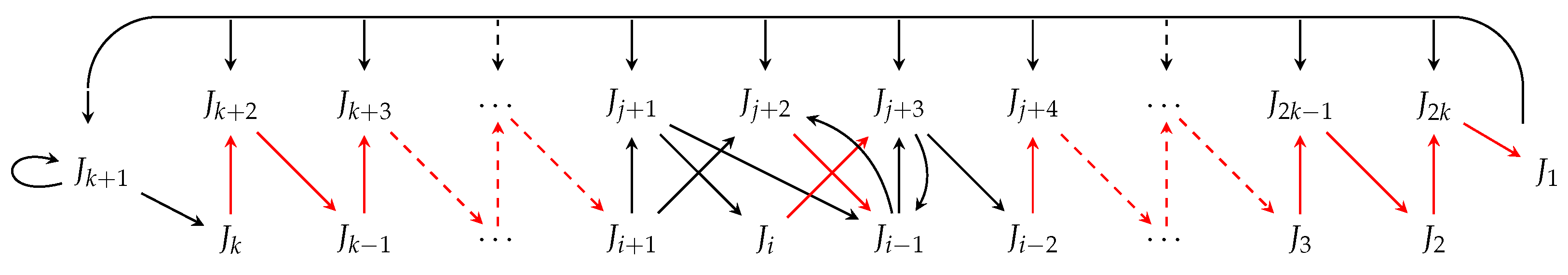
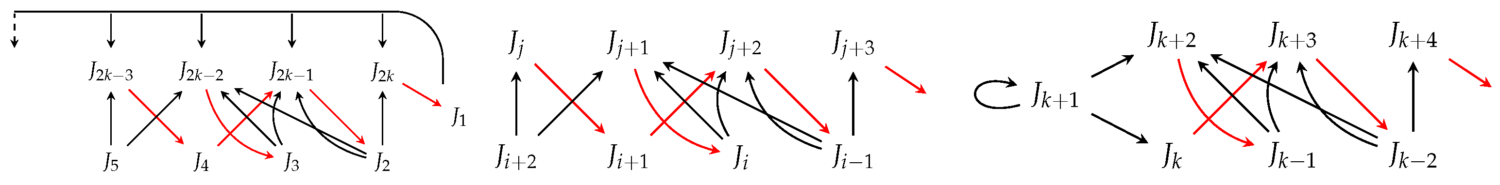
• Case $\left(2\right)$: $f(2k+1)=1\Rightarrow f\left(2k\right)=1,f\left(1\right)=2k+1,f\left(3\right)=2k$; this leads to a valid second minimal orbit with the topological structure min-max and the associated digraph is presented in Figure 12 and the cyclic permutation is listed in (15). Next, we prove as in previous case that there are no primitive cycles of even length $\le 2k-2$, and, therefore, according to Lemms 3, P-linearization of the orbit (14) presents an example of a continuous map with a second minimal $(2k+1)$-orbit.

  (a)

  Consider primitive cycles that contain $J_1$. Without any loss of generality, choose $J_1$ as the starting vertex. First, assume that the cycle does not contain $J_{k+1}$. Since $J_{2k+1-i}\to J_i,$$i=1,\dots ,k-1,$ any such cycle can be formed only by adding to starting vertex $J_1$ pairs $(J_{2k+1-i},J_i),i=1,\dots ,k-1$. Therefore, the length of the cycle (by counting $J_1$ twice) will be always an odd number. Conversely, if the cycle contains $J_{k+1}$, then to close it at $J_1$, the smallest required even length is $2k+2$.

  (b)

  Consider primitive cycles that do not contain $J_1$, but contain $J_2$. Without any loss of generality, choose $J_2$ as the starting vertex. First, assume that the cycle does not contain $J_{k+1}$. Since $J_{2k+1-i}\to J_i,i=2,\dots ,k-1,$ any such cycle can be formed only by adding to starting vertex $J_2$ pairs $(J_{2k+1-i},J_i),i=2,\dots ,k-1$. Therefore, the length of the cycle (by counting $J_2$ twice) will be always an odd number. Conversely, if the cycle contains $J_{k+1}$, then to close it at $J_2$, the smallest required even length is $2k$. Finally, it is easy to see that by excluding $J_1$ and $J_2$ from the cycle, due to the red edges, all the vertices but $J_{k+1}$ must be also excluded, and cycle at $J_{k+1}$ is the only possibility.

• Case $\left(3\right)$: $f(2k+1)=2k\Rightarrow f\left(3\right)=2k+1,f\left(1\right)=2,f\left(2k\right)=1$. The produced cyclic permutation contains the subgraph $J_{2k}\to J_1\to J_3\to J_{2k}$. According to Straffin’s lemma this subgraph implies the existence of a period 3-orbit, which is a contradiction.

□

Lemma 7. 

Placing $\tilde{J}$ and $\widehat{J}$ in setting $(2,2k-1)$ produces exactly 3 second minimal orbits. These are given in listings (14), (18), and (19) and the corresponding digraphs are presented in Figure 11, Figure 14, and Figure 15, respectively.

$$\left(\begin{array}{ccccccccccc}1& 2& 3& 4& \cdots & k+1& k+2& \cdots & 2k-1& 2k& 2k+1\\ k+1& 2k& 2k+1& 2k-1& \cdots & k+2& k& \cdots & 3& 1& 2\end{array}\right)$$

(18)

$$\left(\begin{array}{ccccccccccc}1& 2& 3& \cdots & k+1& k+2& \cdots & 2k-2& 2k-1& 2k& 2k+1\\ k+1& 2k+1& 2k& \cdots & k+2& k& \cdots & 4& 2& 1& 3\end{array}\right)$$

(19)

Proof. 

Having inserted $(\tilde{J},\widehat{J})$ in position $(2,2k-1)$ and by using the path (7) and the rules in (8) and (9), we observe that the images of the elements of the cycle from 4 to $2k-2$ are uniquely defined following a Stefan structure as demonstrated in (20).

$$\left(\begin{array}{ccccccc}4& \cdots & k& k+1& k+2& \cdots & 2k-2\\ 2k-1& \cdots & k+3& k+2& k& \cdots & 4\end{array}\right)$$

(20)

The alteration appears only in images of the elements $1,2,3,2k-1,2k+1$. By using the path (7) and the rules in (8) and (9) again, we construct the potential cyclic permutation (21) and analyze which of the available choices lead to valid second minimal odd orbits.

$$\left(\begin{array}{ccccccccc}1& 2& 3& \cdots & k+1& \cdots & 2k-1& 2k& 2k+1\\ \langle k+1,& \begin{array}{c}2k+1\\ 2k\end{array}\rangle & \begin{array}{c}2k\\ 2k+1\end{array}& \cdots & k+2& \cdots & \begin{array}{c}2\\ 3\end{array}& 1& \begin{array}{c}3\\ 2\end{array}\end{array}\right)$$

(21)

• If $f\left(1\right)=2k\Rightarrow 2$-suborbit $\left\{1,2k\right\}$, a contradiction.
• If $f\left(1\right)=2k+1\Rightarrow f\left(2\right)=k+1,f\left(3\right)=2k$

  (a)

  If $f(2k-1)=2\Rightarrow f(2k+1)=3\Rightarrow 4$-suborbit $\left\{1,3,2k,2k+1\right\}$, a contradiction.

  (b)

  If $f(2k-1)=3\Rightarrow f(2k+1)=2$, but we have a second minimal $(2k+1)$ orbit given in (14) with topological structure min-max-min, observe that this is the same as (14) from setting $(1,2k-1)$, and so the settings share a cyclic permutation. This is expected since to move from setting $(1,2k-1)$ to $(2,2k-1)$, only the location of $\tilde{J}$ is changed and so, in this particular case, the digraph remains unchanged as we simply swap the intervals $\tilde{J}$ and $J_{r_{2k-2}}$.

• $f\left(1\right)=k+1,f\left(2\right)=2k\Rightarrow f\left(3\right)=2k+1,f(2k+1)=2,f(2k-1)=3.$ This leads to a valid second minimal orbit with the topological structure max-min and the associated digraph is presented in Figure 14 and the cyclic permutation is listed in (18). Next, we prove that there are no primitive cycles of even length $\le 2k-2$, and therefore according to Lemma 3, P-linearization of the orbit (18) presents an example of a continuous map with a second minimal $(2k+1)$-orbit.

  (a)

  Consider primitive cycles that contain $J_1$. Without any loss of generality, choose $J_1$ as the starting vertex. First, assume that the cycle does not contain $J_{k+1}$. Since $J_{2k+1-i}\to J_i,$$i=1,\dots ,k-1;i\ne 2;$ and $J_{2k-1}\to J_1,J_{2k-1}\to J_2$, any such cycle can be formed only by adding to starting vertex $J_1$ pairs $(J_{2k-1},J_2)$, $(J_{2k+1-i},J_i),i=1,\dots ,k-1$. Therefore, the length of the cycle (by counting $J_1$ twice) will be always an odd number. Conversely, if the cycle contains $J_{k+1}$, then to close it at $J_1$, the smallest required even length is $2k$.

  (b)

  Consider primitive cycles that do not contain $J_1$. It is easy to see that by excluding $J_1$ from the cycle, due to the red edges, all the vertices but $J_{k+1}$ must also be excluded, and the cycle at $J_{k+1}$ is the only possibility.

• $f\left(1\right)=k+1,f\left(2\right)=2k+1\Rightarrow f\left(3\right)=2k,f(2k+1)=3,f(2k-1)=2$. This produces a second minimal $(2k+1)$ orbit with topological structure max-min and the associated digraph is presented in Figure 15 and the cyclic permutation is listed in (19). As in previous cases, we prove that there are no primitive cycles of even length $\le 2k-2$, and therefore according to Lemma 3, P-linearization of the orbit (19) presents an example of a continuous map with a second minimal $(2k+1)$-orbit.

  (a)

  Consider primitive cycles that contain $J_1$. Without any loss of generality, choose $J_1$ as the starting vertex. First, assume that the cycle does not contain $J_{k+1}$. Since $J_{2k+1-i}\to J_i,i=4,\dots ,k-1$ (if $k\ge 5$) and $J_{2k-2}\to J_3$, $J_{2k-2}\to J_2$, $J_{2k-1}\to J_1$, $J_{2k}\to J_1$, any such cycle can be formed only by adding to starting vertex $J_1$ pairs $(J_{2k-1},J_1)$, $(J_{2k},J_2)$, $(J_{2k-2},J_2)$, $(J_{2k+1-i},J_i),$$i=1,\dots ,k-1;i\ne 2;$ Therefore, the length of the cycle (by counting $J_1$ twice) will always be an odd number. Conversely, if the cycle contains $J_{k+1}$, then to close it at $J_1$ the smallest required even length is $2k$.

  (b)

  Consider primitive cycles that do not contain $J_1$. It is easy to see that by excluding $J_1$ from the cycle, due to the red edges, all the vertices but $J_{k+1},J_{2k},J_2$ must be also excluded, and a cycle at $J_{k+1}$ and a cycle formed by $J_2$ and $J_{2k}$ are the only possibilities.

□

Lemma 8. 

Placing $\tilde{J}$ and $\widehat{J}$ in setting $(2,2k-2)$ produces exactly 4 second minimal orbits. These are listed in cyclic permutations (15), (18), (22), and (23) and the corresponding digraphs are presented in Figure 12, Figure 14, Figure 16, and Figure 17, respectively.

$$\left(\begin{array}{cccccccccccc}1& 2& 3& 4& \cdots & k+1& k+2& \cdots & 2k-2& 2k-1& 2k& 2k+1\\ k+1& 2k& 2k+1& 2k-1& \cdots & k+2& k& \cdots & 4& 2& 3& 1\end{array}\right)$$

(22)

$$\left(\begin{array}{cccccccccccc}1& 2& 3& 4& 5& \cdots & k+1& k+2& \cdots & 2k-1& 2k& 2k+1\\ k+1& 2k-1& 2k+1& 2k& 2k-2& \cdots & k+2& k& \cdots & 3& 2& 1\end{array}\right)$$

(23)

Proof. 

Having inserted $(\tilde{J},\widehat{J})$ in position $(2,2k-2)$ and by using the path (7) and the rules in (8) and (9), we observe that the images of the elements of the cycle from 5 to $2k-2$ are uniquely defined following a Stefan structure as demonstrated in (24).

$$\left(\begin{array}{ccccccc}5& \cdots & k& k+1& k+2& \cdots & 2k-2\\ 2k-2& \cdots & k+3& k+2& k& \cdots & 4\end{array}\right)$$

(24)

The alteration appears only in images of the elements $1,2,4,2k-1,2k,2k+1$. By using the path (7) and the rules in (8) and (9) again, we construct the potential cyclic permutation (25) and analyze which of the available choices lead to valid second minimal odd orbits.

$$\left(\begin{array}{cccccccc}1& 2& 3& 4& \cdots & 2k-1& 2k& 2k+1\\ \langle k+1,& \begin{array}{c}2k-1\\ 2k\end{array}\rangle & 2k+1& \begin{array}{c}2k\\ 2k-1\end{array}& \cdots & \begin{array}{c}2\\ 3\end{array}& \langle 1,& \begin{array}{c}3\\ 2\end{array}\rangle \end{array}\right)$$

(25)

• If $f\left(1\right)=2k\Rightarrow f\left(2\right)=k+1,f\left(4\right)=2k-1$

  (a)

  If $f\left(2k\right)=1\Rightarrow 2$-suborbit $\left\{1,2k\right\}$, a contradiction.

  (b)

  If $f\left(2k\right)=2$, we have a second minimal $(2k+1)$ orbit given in (15) with topological structure min-max, shared with setting $(1,2k-1)$.

  (c)

  If $f\left(2k\right)=3\Rightarrow 4$-suborbit $\left\{1,3,2k,2k+1\right\}$, a contradiction.

• If $f\left(1\right)=2k-1\Rightarrow f\left(2\right)=k+1,f\left(4\right)=2k$

  (a)

  If $f\left(2k\right)=1$ and $f(2k-1)=2\Rightarrow f(2k+1)=3\Rightarrow 2$-suborbit $\left\{3,2k+1\right\}$, a contradiction.

  (b)

  If $f\left(2k\right)=1$ and $f(2k-1)=3\Rightarrow f(2k+1)=2$, then for $k>3$, we have the primitive subgraph

  $$J_{r_1}\to J_{r_1}\to \cdots \to J_{r_{2k-6}}\to \widehat{J}\to J_{r_{2k-2}}\to J_{r_1}$$

  Lemma 2 implies the existence of a $2k-3$-periodic orbit, which is a contradiction. For $k=3$, we have the subgraph

  $$J_{r_1}\to \widehat{J}\to J_{r_4}\to J_{r_1}$$

  which leads to a 3-orbit, a contradiction.

  (c)

  If $f\left(2k\right)=2\Rightarrow f(2k-1)=3,f(2k+1)=1\Rightarrow 4$-suborbit $\left\{1,3,2k-1,2k+1\right\}$, a contradiction.

  (d)

  If $f\left(2k\right)=3\Rightarrow f(2k-1)=2,f(2k+1)=1$, then for $k>3$, we have the subgraph

  $$J_{r_1}\to J_{r_1}\to \cdots \to J_{r_{2k-6}}\to \widehat{J}\to \tilde{J}\to J_{r_1}$$

  Lemma 2 implies the existence of a $2k-3$-periodic orbit, which is a contradiction. For $k=3$, we have the subgraph

  $$J_{r_1}\to \widehat{J}\to \tilde{J}\to J_{r_1}$$

  which leads to a 3-orbit, a contradiction.

• If $f\left(2\right)=2k\Rightarrow f\left(1\right)=k+1,f\left(4\right)=2k-1$

  (a)

  If $f\left(2k\right)=1$ and $f(2k-1)=2\Rightarrow f(2k+1)=3\Rightarrow 2$-suborbit $\left\{3,2k+1\right\}$, a contradiction.

  (b)

  If $f\left(2k\right)=1$ and $f(2k-1)=3\Rightarrow f(2k+1)=2$, we have a second minimal $(2k+1)$ orbit given in (18) with topological structure max-min, shared with setting $(2,2k-1)$.

  (c)

  If $f\left(2k\right)=2\Rightarrow 2$-suborbit $\left\{2,2k\right\}$, a contradiction.

  (d)

  If $f\left(2k\right)=3\Rightarrow f(2k-1)=2,f(2k+1)=1$, we have a second minimal $(2k+1)$ orbit given in (22) with topological structure max-min-max, and the associated digraph is presented in Figure 16. Next we prove as in previous lemma that there are no primitive cycles of even length $\le 2k-2$, and therefore according to Lemma 3, P-linearization of the orbit (22) presents an example of a continuous map with a second minimal $(2k+1)$-orbit.

  i.

  Consider primitive cycles that contain $J_1$. Without any loss of generality, choose $J_1$ as the starting vertex. First, assume that the cycle does not contain $J_{k+1}$. Since $J_{2k+1-i}\to J_i,i=2,\dots ,k-1;i\ne 3;$ and $J_{2k}\to J_1,J_{2k-2}\to J_3$, $J_{2k-2}\to J_2$, any such cycle can be formed only by adding to starting vertex $J_1$ pairs $(J_{2k-2},J_2)$, $(J_{2k+1-i},J_i),i=1,\dots ,k-1$. Therefore, the length of the cycle (by counting $J_1$ twice) will be always an odd number. Conversely, if the cycle contains $J_{k+1}$, then to close it at $J_1$, the smallest required even length is $2k$.

  ii.

  Consider primitive cycles that do not contain $J_1$. It is easy to see that by excluding $J_1$ from the cycle, due to the red edges, all the vertices but $J_{k+1},J_2,J_{2k}$ must be also excluded, and a cycle at $J_{k+1}$ and a cycle formed by $J_2$ and $J_{2k}$ are the only possibilities.

• If $f\left(2\right)=2k-1\Rightarrow f\left(1\right)=k+1,f\left(4\right)=2k$

  (a)

  If $f\left(2k\right)=1$ and $f(2k-1)=2\Rightarrow 2$-suborbit $\left\{2,2k-1\right\}$, a contradiction.

  (b)

  If $f\left(2k\right)=1$ and $f(2k-1)=3\Rightarrow 4$-suborbit $\left\{2,3,2k-1,2k+1\right\}$, a contradiction.

  (c)

  If $f\left(2k\right)=2\Rightarrow f(2k-1)=3,f(2k+1)=1$, we have a second minimal $(2k+1)$ orbit given in (23) with topological structure max-min-max, and the associated digraph is presented in Figure 17. Next, we prove as in previous cases that there are no primitive cycles of even length $\le 2k-2$, and therefore according to Lemma 3, P-linearization of the orbit (23) presents an example of a continuous map with a second minimal $(2k+1)$-orbit.

  (i)

  Consider primitive cycles that contain $J_1$. Without any loss of generality, choose $J_1$ as the starting vertex. First, assume that the cycle does not contain $J_{k+1}$. Since $J_{2k+1-i}\to J_i,i=1,\dots ,k-1,$ any such cycle can be formed only by adding to starting vertex $J_1$ pairs $(J_{2k+1-i},J_i), i=1,\dots ,k-1$. Therefore, the length of the cycle (by counting $J_1$ twice) will be always an odd number. Conversely, if the cycle contains $J_{k+1}$, then to close it at $J_1$, the smallest required even length is $2k$.

  (ii)

  Consider primitive cycles that do not contain $J_1$. It is easy to see that by excluding $J_1$ from the cycle, due to the red edges, all the vertices but $J_{k+1},J_2,J_{2k-1}$ must be also excluded, and a cycle at $J_{k+1}$ and a cycle formed by $J_2$ and $J_{2k-1}$ are the only possibilities.

  (d)

  If $f\left(2k\right)=3\Rightarrow f(2k-1)=2\Rightarrow 2$-suborbit $\left\{2,2k-1\right\}$, a contradiction.

□

Lemma 9. 

Each setting $(i,j)$ with $2<i<k$ and $j=2k-i,k>3$ produces exactly 4 second minimal cycles listed in cyclic permutations (26), (27), (28), and (29). If $i=3$, (26) repeats the cyclic permutation (23) revealed in Lemma 8. When $i=k-1$, the cyclic permutation (29) and (10) from Lemma 4 are identical. The corresponding digraphs are presented in Figure 18, Figure 19, Figure 20, and Figure 21, respectively, when $3<i<k-1$.

$$\left(\begin{array}{cccccccccccc}1& \cdots & i-1& i& i+1& i+2& \cdots & j+1& j+2& j+3& \cdots & 2k+1\\ k+1& \cdots & j+2& j+4& j+3& j+1& \cdots & i+1& i& i-1& \cdots & 1\end{array}\right)$$

(26)

$$\left(\begin{array}{cccccccccccc}1& \cdots & i-1& i& i+1& i+2& \cdots & j+1& j+2& j+3& \cdots & 2k+1\\ k+1& \cdots & j+4& j+2& j+3& j+1& \cdots & i& i+1& i-1& \cdots & 1\end{array}\right)$$

(27)

$$\left(\begin{array}{cccccccccccc}1& \cdots & i-1& i& i+1& i+2& \cdots & j+1& j+2& j+3& \cdots & 2k+1\\ k+1& \cdots & j+4& j+2& j+3& j+1& \cdots & i+1& i-1& i& \cdots & 1\end{array}\right)$$

(28)

$$\left(\begin{array}{cccccccccccc}1& \cdots & i-1& i& i+1& i+2& \cdots & j+1& j+2& j+3& \cdots & 2k+1\\ k+1& \cdots & j+4& j+1& j+3& j+2& \cdots & i+1& i& i-1& \cdots & 1\end{array}\right)$$

(29)

Proof. 

We prove this by doing a case by case analysis of the general cyclic permutation listed in (30).

$$\left(\begin{array}{cccccccccc}\cdots & i-1& i& i+1& i+2& \cdots & j+1& j+2& j+3& \cdots \\ \cdots & <\begin{array}{c}j+2\\ j+1\end{array},& j+4>& j+3& \begin{array}{c}j+1\\ j+2\end{array}& \cdots & \begin{array}{c}i+1\\ i\end{array}& <\begin{array}{c}i\\ i+1\end{array},& i-1>& \cdots \end{array}\right)$$

(30)

• If $f(i-1)=j+2\Rightarrow f\left(i\right)=j+4,f(i+2)=j+1$

  (a)

  If $f(j+2)=i-1\Rightarrow 2$-suborbit $\left\{i-1,j+2\right\}$, a contradiction.

  (b)

  If $f(j+2)=i+1\Rightarrow 4$-suborbit $\left\{i-1,i+1,j+2,j+3\right\}$, a contradiction.

  (c)

  If $f(j+2)=i$, we have a second minimal $(2k+1)$ orbit given in (26) with topological structure max-min-max, provided $i>3$. If $i=3$, then we have a second minimal $2k+1$-orbit (23) with topological structure max revealed in Lemma 8.

• If $f(i-1)=j+1\Rightarrow f\left(i\right)=j+4,f(i+2)=j+2$

  (a)

  If $f(j+1)=i+1\Rightarrow 4$-suborbit $\left\{i-1,i+1,j+1,j+3\right\}$, a contradiction.

  (b)

  If $f(j+1)=i\Rightarrow f(j+3)\ne i+1$ or we have the closed 2-suborbit $\left\{i+1,j+3\right\}$. So we must have $f(j+3)=i-1\Rightarrow f(j+2)=i+1$. Following the proof of Lemma 5, it follows that for $2<i<k-1$, the digraph of the cyclic permutation contains a primitive subgraph

  $$J_{r_1}\to J_{r_2}\to \cdots \to J_{r_{w-4}}\to \widehat{J}\to \tilde{J}\to J_{r_{w+1}}\to \cdots \to J_{r_{2k-2}}\to J_{r_1}\to J_{r_1}$$

  and for $i=k-1$, the digraph of the cyclic permutation contains a primitive subgraph

  $$J_{r_1}\to \widehat{J}\to \tilde{J}\to J_{r_5}\to \cdots \to J_{r_{2k-2}}\to J_{r_1}$$

  both of which have length $2k-2$. By Lemma 2, a periodic orbit of period $2k-3$ must exist, which is a contradiction.

  (c)

  If $f(j+1)=i+1\Rightarrow f(j+3)\ne i-1$ or there is a period 4-suborbit $i-1,i+1$, $j+1,j+3$. Thus, $f(j+3)=i\Rightarrow f(j+2)=i-1$. By repeating the argument of the previous case, we prove the existence of the $2k-3$-orbit, which is a contradiction.

• If $f\left(i\right)=j+2\Rightarrow f(i-1)=j+4,f(i+2)=j+1$

  (a)

  If $f(j+2)=i\Rightarrow$ closed 2-suborbit $\left\{i,j+2\right\}$, a contradiction.

  (b)

  If $f(j+2)=i+1\Rightarrow f(j+1)=i,f(j+3)=i-1$, we have a second minimal $(2k+1)$ orbit given in (27) with topological structure max-min-max-min-max.

  (c)

  If $f(j+2)=i-1$ and $f(j+3)=i+1\Rightarrow$ closed 2-suborbit $\left\{i+1,j+3\right\}$, a contradiction.

  (d)

  If $f(j+2)=i-1,f(j+3)=i\Rightarrow f(j+1)=i+1$, we have a second minimal $(2k+1)$ orbit given in (28) with topological structure max-min-max-min-max.

• If $f\left(i\right)=j+1\Rightarrow f(i-1)=j+4,f(i+2)=j+2$

  (a)

  If $f(j+1)=i\Rightarrow 2$-suborbit $\left\{i,j+1\right\}$, a contradiction.

  (b)

  If $f(j+1)=i+1$ and $f(j+3)=i\Rightarrow 4$-suborbit $\left\{i,i+1,j+1,j+3\right\}$, a contradiction.

  (c)

  If $f(j+1)=i+1$ and $f(j+3)=i-1$, we have a second minimal $(2k+1)$ orbit given in (29) with topological structure max-min-max, unless $i=3$, in which case the topological structure is single max. When $i=k-1$, the cyclic permutation (29) repeats the cyclic permutation (10) revealed in Lemma 4.

Observe, as i varies between 3 and $k-1$, the structure of the digraphs associated with the cyclic permutations changes. In particular, for a given cyclic permutation, varying i from 3 to $k-1$ shifts the region of variations from the right to left end of the digraph. We demonstrate this in Figure 22, Figure 23, Figure 24 and Figure 25. Note that in these subgraphs, with the exception of Figure 22a, where $J_1\cancel{\to }{J}_{2k-1},J_{2k}$, we have $J_1\to J_{k+1},\dots ,J_{2k}$.

Note that all four cyclic permutations are simple. Next, we analyze the digraphs to show that there are no primitive cycles of even length $\le 2k-2$, which would imply by Straffin’s lemma, an existence of an odd periodic orbit of length $\le 2k-3$. From Lemms 3, it then follows that the P-linearization of the orbits (26), (27), (28), and (29) present an example of a continuous map with a second minimal $(2k+1)$-orbit. The proof coincides with the similar proofs given in previous lemmas.

• Consider primitive cycles that contain $J_1$. Without any loss of generality, choose a starting vertex as $J_1$. First, assume that the cycle does not contain $J_{k+1}$. Due to presence of red edges, any such cycle can be formed only by successfully adding to starting vertex $J_1$ pairs $(J_p,J_q)$, where $q\in \{1,\dots ,k-1\}$, $p\in \{k+2,\dots ,2k\}$. Therefore, the length of the cycle (by counting $J_1$ twice) will be always an odd number. Conversely, if the cycle contains $J_{k+1}$, then, besides the new pair $(J_{k+1},J_k)$ or $(J_{k+1},J_{k-1})$ there is a possibility to add just $J_{k+1}$ alone due to the loop at $J_{k+1}$, and hence, to build a primitive subgraph of even length. However, the smallest required even length is $2k$, and, therefore, no odd orbits of a period smaller than $2k-1$ can be produced.
• Consider primitive cycles that do not contain $J_1$. Since $J_1\to J_{k+1}$ and $J_{k+1}\to J_{k+1}$ are only edges directed to $J_{k+1}$, we have to exclude $J_{k+1}$ from the primitive cycle unless it is a loop at $J_{k+1}$. However, then, any primitive cycle formed by the remaining intervals can be formed by adding some of the indicated pairs $(J_p,J_q)$ to the starting vertex, and, therefore, all are of odd length.

□

Lemma 10. 

Each setting $(i,j+1)$ with $2<i<k$ and $j=2k-i,k>3$ produces exactly 4 second minimal cycles listed in cyclic permutations (31), (32), (33), and (34). Cyclic permutation (32) repeats (28) from Lemma 9. If $i=3$, (31) repeats the cyclic permutation (22) revealed in Lemma 8, and (34) repeats the cyclic permutation (19) revealed in Lemma 7. The corresponding digraphs are presented in Figure 26, Figure 27, Figure 28 and Figure 29, respectively.

$$\left(\begin{array}{ccccccccccc}1& \cdots & i-1& i& i+1& \cdots & j+1& j+2& j+3& j+4& \cdots \\ k+1& \cdots & j+3& j+4& j+2& \cdots & i+1& i-1& i& i-2& \cdots \end{array}\right)$$

(31)

$$\left(\begin{array}{ccccccccccc}1& \cdots & i-1& i& i+1& \cdots & j+1& j+2& j+3& j+4& \cdots \\ k+1& \cdots & j+4& j+2& j+3& \cdots & i+1& i-1& i& i-2& \cdots \end{array}\right)$$

(32)

$$\left(\begin{array}{ccccccccccc}1& \cdots & i-1& i& i+1& \cdots & j+1& j+2& j+3& j+4& \cdots \\ k+1& \cdots & j+4& j+3& j+2& \cdots & i& i-1& i+1& i-2& \cdots \end{array}\right)$$

(33)

$$\left(\begin{array}{ccccccccccc}1& \cdots & i-1& i& i+1& \cdots & j+1& j+2& j+3& j+4& \cdots \\ k+1& \cdots & j+4& j+3& j+2& \cdots & i+1& i-1& i-2& i& \cdots \end{array}\right)$$

(34)

Proof. 

We prove this by doing a case by case analysis of the general cyclic permutation listed in (35).

$$\left(\begin{array}{cccccccccc}\cdots & i-1& i& i+1& \cdots & j+1& j+2& j+3& j+4& \cdots \\ \cdots & <\begin{array}{c}j+2\\ j+3\end{array},& j+4>& \begin{array}{c}j+3\\ j+2\end{array}& \cdots & \begin{array}{c}i+1\\ i\end{array}& i-1& <\begin{array}{c}i\\ i+1\end{array},& i-2>& \cdots \end{array}\right)$$

(35)

• If $f(i-1)=j+2\Rightarrow 2$-suborbit $\left\{i-1,j+2\right\}$, a contradiction.
• If $f(i-1)=j+3\Rightarrow f\left(i\right)=j+4,f(i+1)=j+2$

  (a)

  If $f(j+3)=i\Rightarrow f(j+1)=i+1,f(j+4)=i-2$, we have a second minimal $(2k+1)$ orbit given in (31) with topological structure max-min-max-min-max, if $i>3$. If $i=3$, then we have a second minimal $2k+1$-orbit (22) with topological structure max-min-max revealed in Lemma 8.

  (b)

  If $f(j+3)=i+1\Rightarrow 4$-suborbit $\left\{i-1,i+1,j+2,j+3\right\}$, a contradiction.

  (c)

  If $f(j+3)=i-2$ and $f(j+4)=i\Rightarrow 2$-suborbit $\left\{i,j+4\right\}$, a contradiction.

  (d)

  If $f(j+3)=i-2$ and $f(j+4)=i+1\Rightarrow f(j+1)=i$. Following the proof of the Lemma 5, it follows that for $2<i<k-1$, the digraph of the cyclic permutation contains a primitive subgraph

  $$J_{r_1}\to J_{r_2}\to \cdots \to J_{r_{w-3}}\to \tilde{J}\to \widehat{J}\to J_{r_{w+2}}\to J_{r_{w+3}}\to \cdots \to J_{r_{2k-2}}\to J_{r_1}\to J_{r_1}$$

  and for $i=k-1$, the digraph of the cyclic permutation contains a primitive subgraph

  $$J_{r_1}\to \tilde{J}\to \widehat{J}\to J_{r_6}\to \cdots \to J_{r_{2k-2}}\to J_{r_1}\to J_{r_1}$$

  both of which have length $2k-2$. By Lemma 2, a periodic orbit of period $2k-3$ must exist, which is a contradiction.

• If $f\left(i\right)=j+2\Rightarrow f(i-1)=j+4,f(i+1)=j+3$

  (a)

  If $f(j+3)=i\Rightarrow f(j+1)=i+1,f(j+4)=i-2$, we have a second minimal $(2k+1)$ orbit given in (32) with topological structure max-min-max-min-max. Cyclic permutation (32) repeats (28) from Lemma 9.

  (b)

  If $f(j+3)=i+1\Rightarrow 2$-suborbit $\left\{i+1,j+3\right\}$, a contradiction.

  (c)

  If $f(j+3)=i-2$ and $f(j+4)=i+1\Rightarrow f(j+1)=i$. This implies a cyclic permutation whose digraph contains a primitive subgraph of length $2k-2$. The proof coincides with the proof given above in the case (2d). By Lemma 2, a periodic orbit of period $2k-3$ must exist, which is a contradiction.

  (d)

  If $f(j+3)=i-2$ and $f(j+4)=i\Rightarrow f(j+1)=i+1\Rightarrow 4$-suborbit $\left\{i,i-1,j+2,j+4\right\}$, a contradiction.

• If $f\left(i\right)=j+3\Rightarrow f(i-1)=j+4,f(i+1)=j+2$

  (a)

  If $f(j+3)=i\Rightarrow 2$-suborbit $\left\{i,j+3\right\}$, a contradiction.

  (b)

  If $f(j+3)=i+1\Rightarrow f(j+1)=i,f(j+4)=i-2$, we have a second minimal $(2k+1)$ orbit given in (33) with topological structure max-min-max.

  (c)

  If $f(j+3)=i-2$ and $f(j+4)=i+1\Rightarrow 4$-suborbit $\left\{i-1,i+1,j+2,j+4\right\}$, a contradiction.

  (d)

  If $f(j+3)=i-2$ and $f(j+4)=i\Rightarrow f(j+1)=i+1$, we have a second minimal $(2k+1)$ orbit given in (34) with topological structure max-min-max, if $i>3$. If $i=3$, then we have a second minimal $2k+1$-orbit (19) with topological structure max-min revealed in Lemma 7.

As i varies between 3 and $k-1$, the structure of the digraphs associated with the cyclic permutations changes. In particular, for a given cyclic permutation, varying i from 3 to $k-1$ shifts the region of variations from the right to left end of the digraph. We demonstrate this in Figure 30, Figure 31, Figure 32 and Figure 33. Observe that Figure 24 and Figure 31 are identical. Note that in these subgraphs, with the exception of Figure 30 where $J_1\cancel{\to }{J}_{2k}$, we have $J_1\to J_{k+1},\dots ,J_{2k}$.

Note that all four cyclic permutations are simple. Finally, we aim to analyze the digraphs and demonstrate that there are no primitive cycles of even length $\le 2k-2$, which would imply by Straffin’s lemma, an existence of an odd periodic orbit of length $\le 2k-3$. From Lemms 3, it then follows that the P-linearization of the orbits (31), (32), (33), and (34) present an example of a continuous map with a second minimal $(2k+1)$-orbit. The proof coincides with the similar proof given in Lemma 9. □

Lemma 11. 

Placing $(\tilde{J},\widehat{J})$ in relative positions $(k,k+1)$ produces exactly 4 second minimal cycles, listed in cyclic permutations (36), (37), (38), and (39). The corresponding digraphs are presented in Figure 34, Figure 35, Figure 36 and Figure 37, respectively.

$$\left(\begin{array}{ccccccccccc}1& 2& \cdots & k-1& k& k+1& k+2& k+3& k+4& \cdots & 2k+1\\ k+1& 2k+1& \cdots & k+4& k+2& k+3& k-1& k& k-2& \cdots & 1\end{array}\right)$$

(36)

$$\left(\begin{array}{cccccccccccc}1& 2& \cdots & k-1& k& k+1& k+2& k+3& k+4& k+5& \cdots & 2k+1\\ k+1& 2k+1& \cdots & k+4& k+3& k+2& k-1& k-2& k& k-3& \cdots & 1\end{array}\right)$$

(37)

$$\left(\begin{array}{ccccccccccc}1& 2& \cdots & k-1& k& k+1& k+2& k+3& k+4& \cdots & 2k+1\\ k& 2k+1& \cdots & k+4& k+3& k+2& k-1& k+1& k-2& \cdots & 1\end{array}\right)$$

(38)

$$\left(\begin{array}{ccccccccccc}1& 2& \cdots & k-1& k& k+1& k+2& k+3& k+4& \cdots & 2k+1\\ k+1& 2k+1& \cdots & k+3& k+4& k+2& k-1& k& k-2& \cdots & 1\end{array}\right)$$

(39)

Proof. 

We prove this by doing a case by case analysis of the general cyclic permutation listed in (35). Note that in the frame of notation introduced in the proof of Lemma 5, we have $w=2$;

$$\left(\begin{array}{ccccccccc}1& \cdots & k-1& k& k+1& k+2& k+3& k+4& \cdots \\ \begin{array}{c}k+1\\ k\end{array}& \cdots & <k+4,& \begin{array}{c}k+3\\ k+2\end{array}>& \begin{array}{c}k+2\\ k+3\end{array}& k-1& <k-2& \begin{array}{c}k\\ k+1\end{array}>& \cdots \end{array}\right)$$

(40)

• If $f\left(k\right)=k+2\Rightarrow f(k-1)=k+4,f(k+1)=k+3$

  (a)

  If $f(k+4)=k\Rightarrow f\left(1\right)=k+1,f(k+3)=k-2\Rightarrow 4$-suborbit $\left\{k-1,k,k+2,k+4\right\}$, a contradiction.

  (b)

  If $f(k+4)=k+1\Rightarrow f\left(1\right)=k,f(k+3)=k-2$, then for $k>3$ we have the primitive subgraph

  $$\tilde{J}\to \widehat{J}\to J_{r_4}\to \cdots \to J_{r_{2k-2}}\to \tilde{J}$$

  of length $2k-2$. Lemma 2 implies the existence of $2k-3$-orbit, which is a contradiction.

  (c)

  If $f(k+4)=k-2$ and $f(k+3)=k$, we have a second minimal $(2k+1)$ orbit given in (36) with topological structure max-min-max-min-max.

  (d)

  If $f(k+4)=k-2$ and $f(k+3)=k+1\Rightarrow 2$-suborbit $\left\{k+1,k+3\right\}$, a contradiction.

• If $f\left(k\right)=k+3\Rightarrow f(k-1)=k+4,f(k+1)=k+2$

  (a)

  If $f(k+4)=k\Rightarrow f\left(1\right)=k+1,f(k+3)=k-2$, we have a second minimal $(2k+1)$ orbit given in (37) with topological structure max-min-max.

  (b)

  If $f(k+4)=k+1\Rightarrow f\left(1\right)=k,f(k+3)=k-2\Rightarrow 4$-suborbit $\left\{k-1,k+1,k+2,k+4\right\}$, a contradiction.

  (c)

  If $f(k+4)=k-2$ and $f(k+3)=k\Rightarrow 2$-suborbit $\left\{k,k+3\right\}$, a contradiction.

  (d)

  If $f(k+4)=k-2$ and $f(k+3)=k+1\Rightarrow f\left(1\right)=k$, we have a second minimal $(2k+1)$ orbit given in (38) with topological structure max-min-max.

• If $f(k-1)=k+2\Rightarrow 2$-suborbit $\left\{k-1,k+2\right\}$, a contradiction.
• If $f(k-1)=k+3\Rightarrow f\left(k\right)=k+4,f(k+1)=k+2$

  (a)

  If $f(k+4)=k\Rightarrow 2$-suborbit $\left\{k,k+4\right\}$, a contradiction.

  (b)

  If $f(k+4)=k+1\Rightarrow f\left(1\right)=k,f(k+3)=k-2$, then for $k>3$ we have the primitive subgraph

  $$\tilde{J}\to \widehat{J}\to J_{r_4}\to \cdots \to J_{r_{2k-2}}\to \tilde{J}$$

  of length $2k-2$ which leads to contradiction as in case (1b).

  (c)

  If $f(k+4)=k-2$ and $f(k+3)=k\Rightarrow f\left(1\right)=k+1$, we have a second minimal $(2k+1)$ orbit given in (39) with topological structure max-min-max-min-max.

  (d)

  If $f(k+4)=k-2$ and $f(k+3)=k+1\Rightarrow 4$-suborbit $\left\{k-1,k+1,k+2,k+3\right\}$, a contradiction.

Note that all four cyclic permutations are simple. Finally, we aim to analyze the digraphs and demonstrate that there are no primitive cycles of even length $\le 2k-2$, which would imply by Straffin’s lemma an existence of odd periodic orbit of length $\le 2k-3$. From Lemma 3, it then follows that the P-linearization of the orbits (36), (37), (38), and (39) present an example of a continuous map with a second minimal $(2k+1)$-orbit. The proof coincides with the similar proof given in Lemma 9. □

Lemma 12. 

Let $\tilde{J},\widehat{J}$ be in setting $(i,2k-i)$ for $2<i<k$. For fixed i, this setting shares one cyclic permutation with the setting $(i-1,2k-i+1)$ and another cyclic permutation with the setting $(i,2k-i+1)$. When $i=k-1$, the setting $(k-1,k+1)$ shares a cyclic permutation with the case when $m=2k-1$ from Lemma 4.

Proof. 

The proof is by direct comparison. Note that if $i>3$, the cyclic permutation (29) is transformed to (26) after substitution $(i,j)$ with $(i-1,j+1)$. If $i=3$, (26) repeats the cyclic permutation (23). Therefore, the setting $(i,2k-i)$ shares one cyclic permutation with $(i-1,2k-i+1)$. We can also see that the cyclic permutations (28) and (32) are identical. So the setting $(i,2k-i)$ also shares a cyclic permutation with the setting $(i,2k-i+1)$. When $i=k-1$, the cyclic permutation (29) and (10) are identical. □

Lemma 13. 

Let $\tilde{J},\widehat{J}$ be in setting $(i,2k-i+1)$ for $3\le i\le k$. For fixed i, this setting shares one cyclic permutation with the setting $(i-1,2k-i+1)$ and another cyclic permutation with the setting $(i-1,2k-i+2)$.

Proof. 

The proof is once again by direct comparison. If $3<i<k$, the substitution $(i,j)$ with $(i-1,j+1)$ in (27) implies the cyclic permutation (31) from Lemma 10. If $i=3$, (31) repeats the cyclic permutation (22), revealed in Lemma 8. If $i=k$, choose $i=k-1$ in the cyclic permutation (27) and observe that it is identical to (39). This proves the sharing with setting $(i-1,2k-i+1)$. Similarly, if $i>3$ the substitution $(i,j)$ with $(i-1,j+1)$ cyclic permutation (33) is transformed to the cyclic permutation (34). If $i=3$ (34) repeats the cyclic permutation (19), revealed in Lemma 7. If $i=k$, then by choosing $i=k-1$ in (33), we see that it is identical to (37). This confirms the sharing with setting $(i-1,2k-i+2)$. □

The sharing mechanism provided in Lemmas 12 and 13 is illustrated in Figure 38. Each setting $(i,2k-i)$ and $(i,2k-i+1),2<i<k$, $(k,k+1)$ contain exactly 4 s minimal cyclic permutations, which are shared with neighboring settings. In particular, for setting $(i,2k-i)$, two cyclic permutations are inherited from its two neighbors immediately to the right, and another two are shared with neighbors immediately below. Observe that we have also demonstrated the sharing extending to the cases $(1,2k-1)$, $(2,2k-1)$, $(2,2k-2)$, and $(k,k+1)$. To count all the different second minimal cyclic permutations, we start in the upper right corner $(1,2k-1)$ of the table in Figure 39 and work our way down to the bottom left corner $(k,k+1)$ by successively moving down and left. Due to the sharing mechanism, the number of new second minimal cyclic permutations produced in each setting is equal to 2 (written as a superscript to the setting). There are $k-1$ columns, each with 4 distinct cycles, giving a total of $4(k-1)$ distinct cyclic permutations. Adding the 1 remaining permutation from Lemma 4, we have the required number, $4k-3$, of second minimal cyclic permutations of period $2k+1$, unique up to an inverse. They are all of the simple positive type according to Definition 1. All the inverse cyclic permutations of the constructed $4k-3$ orbits constitute all the simple negative-type second minimal $2k+1$-orbits. Finally, we count the different types of topological structures of all the $4k-3$ positive-type second minimal orbits and present the results in

Table 2. Counts for topological structure of second minimal odd periodic orbits. Green entries correspond to permutations in settings $(i,2k-i),(i,2k-i+1)$ for $2<i<k$ with $k>3$. Parentheses indicate permutations that may be shared.

Topological Structure	Count	Permutation
max	1	(23)
min-max	1	(15)
min-max-min	1	(14)
max-min	2	(18),(19)
max-min-max	$2k-3$	(11),(22),(38),(26),(29),(33),(34)
max-min-max-min-max	$2k-5$	(36),(27),(31),(28),(32)

. The inverse cyclic permutations have the same topological structures with “max” and “min” exchanged.

5. Conclusions

This paper proves a conjecture on the second minimal odd periodic orbits with respect to Sharkovski ordering for the continuous endomorphisms on the real line. In 1964, in their celebrated paper, Sharkovski discovered a law of coexistence of periodic orbits of the continuous maps on the real line. The law generates a total ordering in $\mathbb{N}$ shown in (1). The structure of the periodic orbits can be characterized through cyclic permutations and directed graphs of transitions or digraphs (Definitions 1 and 2). Remarkably, the structure of the periodic orbits is dictated by the location of the minimal period of the map in the Sharkovski ordering. Stefan (1977) [6] revealed that the minimal odd orbits have a unique cyclic permutation and digraph up to their inverses ((2) and Figure 1). Extending this work, the structure of all the minimal orbits are well understood [7,8]. In this paper, we present a full characterization of the second minimal odd orbits, i.e., orbits with a period being next to the minimal period of the map in the Sharkovski ordering. The main results are the following:

• Second minimal and minimal $2k+1$-orbits ($k\ge 3$) are simple, meaning that elements on the right and left of the central element of the orbit are mapped to each other except one point. We call these positive type (or negative type) if the exceptional element is on the right (or on the left) of the central point. Cyclic permutations and digraphs of all the negative-type simple orbits are inverses of all the positive-type simple orbits, respectively.
• Simple positive-type second minimal $2k+1$-orbits are either Stefan orbits, or have one of the $4k-3$ types, each with a unique digraph and cyclic permutation. Their inverses represent all second minimal $(2k+1)$-orbits of the simple negative type.
• The constructive proof presented in this paper revealed explicitly the cyclic permutations and digrahs of all $4k-3$ second minimal $2k+1$-orbits ($k\ge 3$), as well as their topological structure (Table 1).

The new concept of second minimal orbits and its classification have an important application towards an understanding of the universal structure of the distribution of the periodic windows in the bifurcation diagram generated by the chaotic dynamics of nonlinear maps on the interval. In 1978, Feigenbaum discovered a universal transition mechanism to chaos through successive period doubling bifurcations for the one-parameter family of nonlinear maps with a single quadratic maximum. The revealed scenario of a transition from periodic to chaotic behavior gives a full characterization of the dynamical system in the range of the parameter not exceeding the critical value of the transition to chaos. There has been a long quest to understand the behavior of the dynamical system beyond the transition to chaotic range. A recent paper (Abdulla et al., 2017 [11]) revealed the universal law of the distribution of the periodic windows in the chaotic range of the parameter between the critical value of transition to chaos and the value when a stable 3-orbit appears for the first time. Remarkably, the pattern of distribution of the periodic windows is driven by Sharkovski ordering. In particular, it was revealed that the first appearance of all the odd orbits is always a minimal odd orbit, while the second appearance is the second minimal orbit with a Type I digraph. The reason for the relevance of Type 1 s minimal (2k + 1)-orbits, is due to the fact that the topological structure of the single maximum unimodal map is equivalent to the topological structure of the piecewise monotonic map associated with Type 1 s minimal (2k + 1)-orbits (Table 1).

References

- Sharkovsky, A. Coexistence of cycles of a continuous transofrmation of a line into itself. Ukr. Math. Zh. 1964, 16, 61–71. [Google Scholar]
- Block, L.; Coppel, W.A. Dynamics in One Dimension; Springer: Berlin/Heidelberg, Germany, 1992. [Google Scholar]
- Sharkovsky, A.N.; Maistrenko, Y.L.; Romanenko, E.Y. Difference Equations and Theor Applications; Kluwer Academic Publishers: Dordrecht, The Netherlands, 1986. [Google Scholar]
- Blokh, A.M.; Sharkovsky, O.M. Sharkovsky Ordering; Springer: Cham, Switzerland, 2022; Volume 8, p. 109. [Google Scholar]
- Block, L.; Guckenhimer, J.; Misiurewicz, M.; Young, L. Periodic points and topological entropy of one dimensional maps. In Proceedings of the International Conference on Global Theory of Dynamical Systems, Evanston, IL, USA, 18–22 June 1979; pp. 18–34. [Google Scholar]
- Stefan, P. A theorem of Sharkovskii on the existence of periodic orbits of continuous endomorphisms of the real line. Commun. Math. Phys. 1977, 54, 237–248. [Google Scholar] [CrossRef]
- Alseda, L.; Llibre, J.; Serra, R. Minimal periodic orbits for continuous maps of the interval. Trans. Am. Math. Soc. 1984, 286, 595–627. [Google Scholar] [CrossRef]
- Block, L.; Coppel, W. Stratification of continuous maps of an interval. Trans. Am. Math. Soc. 1986, 297, 587–604. [Google Scholar] [CrossRef]
- Abdulla, A.U.; Abdulla, R.U.; Abdulla, U.G. On the minimal 2(2k + 1)-orbits of the continuous endomorphisms on the real line with application in chaos theory. J. Differ. Equations Appl. 2013, 19, 1395–1416. [Google Scholar] [CrossRef]
- Llibre, J.; Sa, A. Minimal set of periods for continuous self-maps of the eight space. Fixed Point Theory Algorithms Sci. Eng. 2021, 2021, 3. [Google Scholar] [CrossRef]
- Abdulla, U.G.; Abdulla, R.U.; Abdulla, M.U.; Iqbal, N.H. Second minimal orbits, Sharkovski ordering and universality in chaos. Int. J. Bifurc. Chaos 2017, 27, 1730018. [Google Scholar] [CrossRef]
- Feigenbaum, M. Qualitative universality for a class of nonlinear transformations. J. Stat. Phys. 1978, 19, 25–52. [Google Scholar] [CrossRef]
- Feigenbaum, M. The universal metric properties of nonlinear transformations. J. Stat. Phys. 1979, 21, 669–706. [Google Scholar] [CrossRef]
- Feigenbaum, M. Universal behavior in nonlinear systems. Physica 1983, 7, 16–39. [Google Scholar]
- Collet, P.; Eckmann, J.-P.; Lanford, O. Universal properties of maps on an interval. Commun. Math. Phys. 1980, 76, 211–254. [Google Scholar] [CrossRef]
- Campanino, M.; Epstein, H. On the existence of Feigenbaum’s fixed point. Commun. Math. Phys. 1981, 79, 261–302. [Google Scholar] [CrossRef]
- Lanford, O.E. Remarks on the accumulation of period-doubling bifurcations. In Mathematical Problems in Theoretical Physics, Proceedings of the International Conference Mathematics and Physics, Lausanne, Switzerland, 20–25 August 1979; Springer: Berlin/Heidelberg, Germany, 2005; pp. 340–342. [Google Scholar]
- Collet, P.; Eckmann, J.-P. Iterated Maps on the Interval as Dynamical Systems; Birkhauser: Boston, MA, USA, 1980. [Google Scholar]
- Metropolis, N.; Stein, M.L.; Stein, P. On finite limit sets for transformations of the unit interval. J. Comb. Theory 1973, 15, 25–44. [Google Scholar] [CrossRef]
- Milnor, J.; Thurston, W. On iterated maps of the interval. Dyn. Syst. 1988, 1342, 465–563. [Google Scholar]
- Bernhardt, C. Simple permutations with order a power of two. Ergod. Theory Dyn. Syst. 1984, 4, 179–186. [Google Scholar] [CrossRef]
- Acosta-Humanez, P.B. Genealogia de permutaciones simples de orden una potencia de dos. Columbiana Mat. 2008, 2, 1–14. [Google Scholar]
- Acosta-Humanez, P.B.; Martinez-Casablanco, O.E. Simple permutations with order 4n + 2 by means of pasting and reversing. Qual. Theory Dyn. Syst. 2016, 15, 181–210. [Google Scholar] [CrossRef]
- Straffin, P.D. Periodic points of continuous functions. Math. Mag. 1978, 51, 99–105. [Google Scholar] [CrossRef]