Inference for Dependent Competing Risks with Partially Observed Causes from Bivariate Inverted Exponentiated Pareto Distribution Under Generalized Progressive Hybrid Censoring

Abstract

In this paper, inference under dependent competing risk data is considered with multiple causes of failure. We discuss both classical and Bayesian methods for estimating model parameters under the assumption that data are observed under generalized progressive hybrid censoring. The maximum likelihood estimators of model parameters are obtained when occurrences of latent failure follow a bivariate inverted exponentiated Pareto distribution. The associated existence and uniqueness properties of these estimators are established. The asymptotic interval estimators are also constructed. Further, Bayes estimates and highest posterior density intervals are derived using flexible priors. A Monte Carlo sampling algorithm is proposed for posterior computations. The performance of all proposed methods is evaluated through extensive simulations. Moreover, a real-life example is also presented to illustrate the practical applications of our inferential procedures.

1. Introduction

In many lifetime studies, components or systems frequently fail, owing to more than one reason. Thus, analyzing performance of units under isolated failure causes may not always be practicable, which may sometimes lead to lower accuracy and even misleading results. Therefore, various researchers have explored the analysis of failure patterns of systems/components when multiple causes of failure are available in their life cycle. Such inferences are referred to as competing risk models and associated inferences have received reasonable attention in the literature. In traditional studies, statistical inferences are commonly reported under the assumption that causes of failure are treated as independent. Kundu and Basu [1], Sarhan et al. [2], Ghitany et al. [3], Pascual [4], Xu et al. [5], Wang [6], Mahto et al. [7], and Lodhi et al. [8] discuss the competing risk models by considering exponential, Weibull, Lomax, log–normal, Kumaraswamy, Gompertz, and inverted exponentiated distributions. Crowder [9] also presents many useful applications of competing risk models in life testing experiments. However, due to the complex internal structures of systems, the assumption of independent failure modes may not be reasonable in many practical situations (e.g., see Wang et al. [10], Wang et al. [11], and Ashraf et al. [12]). Thus, it may be realistic to make inferences concerning competing risk models when the causes of failure are dependent. For modeling dependent causes, a two- or higher-dimensional probability distribution is usually taken into consideration when analyzing the lifetimes of the units under investigation. As a popular application, Marshall and Olkin [13] proposed the Marshall–Olkin bivariate exponential distribution approach from the perspective of a shock model in their reliability study. This particular model can be extended to some other approaches, like the Marshall–Olkin bivariate Gompertz distribution and the Marshall–Olkin bivariate Weibull distribution. Due to their simpler statistical structure and attractive distributional properties, these lifetime models appear to be very useful. These models have wide-ranging applications in reliability analyses. We further refer to Kaishev et  al. [14], Pena and Gupta [15], Kundu and Gupta [16], Jamalizadeh and Kundu [17], Feizjavadian and Hashemi [18], and Wang et al. [10,11] for useful discussion in this regard.

Often due to time and cost restrictions, it is difficult to conduct lifetime experiments before all testing units have failed. So, information concerning failure times is usually collected in the form of censored data. Here, a test terminates before all the units have failed. In practice, Type-I and Type-II censoring are the most common methods. In such situations, a test is stopped either when a predetermined time is reached or when a predetermined number of failures has been recorded. These schemes do not allow for the removal of live units during experimentation. To overcome such difficulties, progressive censoring schemes are introduced in the literature; here, the removal of units is allowed at various stages of the testing process. Extensive studies have been carried out on traditional and progressive censoring. See, for instance, Panahi and Sayyareh [19], Balakrishnan and Kateri [20], Rastogi and Tripathi [21], and Feroze and Aslam [22] for some recent works. Interested readers may also refer to Balakrishnan and Aggarwala [23] and Lawless [24] for in-depth discussions.

Modern products are usually highly reliable. So, it may still be difficult to collect enough failure samples in traditional and progressive censoring. Cho et al. [25] proposed a new censoring method known as the generalized progressive hybrid censoring (GPHC) scheme; here, testing time can be controlled, and an appropriate number of failure times can be observed under this censoring approach. This method can be briefly described as follows: Let a test begin with n units; further, assume that k and m are prefixed integers satisfying $1\le k\le m\le n$. In addition, non-negative integer-valued variables $r_1,r_2,\dots ,r_m$, and a time point, T, are randomly picked in advance, with $r_1+r_2+\dots +r_m+m=n$. Upon the occurrence of the first failure, say $X_{1:m:n}$, we randomly eliminate $r_1$ number of live units from the test. Similarly, at second failure $X_{2:m:n}$, we randomly remove $r_2$ number of live units from the test. Finally, at the ith failure, $X_{i:m:n}$, we randomly remove $r_i$ number of live units from the test. The experiment stops at time $T^{*}=\max \{X_{k:m:n},\min \{T,X_{m:m:n}\}\}$, i.e.,

$$T^{*}=\left\{\begin{array}{cc}{X}_{k:m:n},\hfill & \mathrm{if}T<X_{k:m:n}<X_{m:m:n}\hfill \\ T,\hfill & \mathrm{if}{X}_{k:m:n}<T<X_{m:m:n}\hfill \\ X_{m:m:n},\hfill & \mathrm{if}{X}_{k:m:n}<X_{m:m:n}<T.\hfill \end{array}\right.$$

Thus, under this scheme, the recorded observations may occur as one of the following three types:

$$\left\{\begin{array}{cc}\mathrm{Case}\mathrm{I}:X_{1:m:n},X_{2:m:n},\dots ,X_{k:m:n},\hfill & \mathrm{if}T<X_{k:m:n}<X_{m:m:n},\hfill \\ \mathrm{Case}\mathrm{II}:X_{1:m:n},\dots ,X_{k:m:n},\dots ,X_{d:m:n},\hfill & \mathrm{if}{X}_{k:m:n}<T<X_{m:m:n},\hfill \\ \mathrm{Case}\mathrm{III}:X_{1:m:n},\dots ,X_{k:m:n},\dots ,X_{m:m:n},\hfill & \mathrm{if}{X}_{k:m:n}<X_{m:m:n}<T,\hfill \end{array}\right.$$

where d satisfies $X_{d:m:n}<T<X_{(d+1):m:n}$. The GPHC scheme encompasses various traditional censoring methods, including Type-I, Type-II, progressive, and hybrid censoring schemes. For completeness, we elucidate the impact of the scheme on the inference process and its advantages in analyzing competing risk data. The GPHC scheme integrates the flexibility of progressive censoring which permits the staggered removal of units during the experiment with a predetermined terminal time, thereby ensuring a balance between study duration and data sufficiency. This affects inference in two pivotal ways. Firstly, the GPHC scheme dynamically adjusts the censoring process based on observed failures, thereby enhancing estimation efficiency compared to fixed-time (Type-I) or fixed-failure (Type-II) censoring schemes. For instance, the likelihood function under the GPHC scheme incorporates both time-dependent failure counts and censoring thresholds, thus facilitating more precise recovery of dependency between parameters in the bivariate model. Secondly, while this scheme introduces complexity into the likelihood formulation due to its adaptive censoring rules, the closed-form survival function of MOBIEP distribution simplifies the derivation of maximum likelihood estimators (MLEs) and the computation of posterior distribution under the Bayesian framework. Additionally, it offers distinct advantages in the context of dependent competing risks. Specifically, competing risks data frequently entail dependencies between failure modes and censoring mechanisms. This particular scheme addresses this by explicitly modeling the joint survival function of MOBIEP distribution, thereby ensuring that the applied scheme adapts to the observed failure patterns without introducing bias into the parameter estimates. It allows early termination of testing if a sufficient number of failures occur. The test can further be extended if more failures need to be recorded. Thus, in various situations, the GPHC scheme optimizes resource allocation. This is particularly beneficial in reliability studies, where prolonged testing may be costly or impractical.

In this paper, we investigate inference procedures for a dependent competing risks model under the assumption that failure times are modeled by a Marshall–Olkin-type bivariate distribution. Various estimates of unknown parameters are derived from both classical and Bayesian viewpoints when latent failure causes follow an inverted exponentiated Pareto (IEP) distribution and failure times are observed under the GPHC scheme with partially detected competing risks.

The remainder of the paper is structured as follows. In Section 2, the proposed Marshall–Olkin bivariate inverted exponentiated Pareto (MOBIEP) model is introduced. The associated competing risk data with partially detected failure causes are also described. Section 3 describes results related to the MLEs of unknown parameters. Additionally, the asymptotic confidence intervals (ACIs) are derived based on the Fisher information matrix. Bayesian point estimates and credible intervals for model parameters are discussed in Section 4. Section 5 provides a numerical study. A real data analysis is also considered for illustrative purposes. Finally, concluding remarks are given in Section 6.

2. Data Description Under Marshall–Olkin-Type Bivariate IEP Model

In this section, the Marshall–Olkin-type bivariate IEP model is proposed for modeling dependent competing risks. Furthermore, data on latent failure times are described under the GPHC scheme.

2.1. Marshall–Olkin Bivariate IEP Distribution

Consider a random variable, X, that follows IEP distribution. Then, its cumulative distribution function (CDF) and the probability density function (PDF) are given by

$$\begin{array}{c}\hfill F_{IEP}(x;\lambda ,\alpha )=1-{\left(1-a{\left(x\right)}^{-\lambda }\right)}^{\alpha },x>0,\end{array}$$

(1)

and

$$\begin{array}{c}\hfill f_{IEP}(x;\lambda ,\alpha )=\lambda \alpha x^{\lambda -1}{(1+x)}^{-(\lambda +1)}{\left(1-a{\left(x\right)}^{-\lambda }\right)}^{\alpha -1},x>0,\end{array}$$

(2)

where $a\left(x\right)=(1+x)/x$. Furthermore, $\alpha >0$ and $\lambda >0$ are shape parameters. The corresponding survival function (SF) of X can be rewritten as

$$\begin{array}{c}\hfill S_{IEP}(x;\lambda ,\alpha )={\left(1-a{\left(x\right)}^{-\lambda }\right)}^{\alpha },x>0.\end{array}$$

(3)

Hereafter, we use notation $IEP(\lambda ,\alpha )$ to denote the inverted exponentiated Pareto distribution with parameters $\lambda$ and $\alpha$. Ghitany et al. [3] presented numerous useful discussions on this model within the context of life test studies. In fact, the authors demonstrated that this particular distribution can appropriately model a variety of physical phenomena. Its hazard rate function may be decreasing or nonmonotone, depending on the values of $\alpha$ and $\beta$. The IEP distribution plays a significant role in life testing and various other practical fields of application, such as communication systems, mortality data analysis, and clinical trials.

Further, the new MOBIEP is constructed as follows. Assume $W_i,i=1,2,3$ are independent random variables, satisfying $W_i\sim IEP(\lambda ,{\alpha }_i)$. Let quantities $T_1=\min (W_1,W_3)$ and $T_2=\min (W_2,W_3)$ be the random vector $(T_1,T_2)$. Then, this pair of random variables is said to follow the MOBIEP distribution with parameters ${\alpha }_1,{\alpha }_2,{\alpha }_3$, and $\lambda$, denoted as $(T_1,T_2)\sim \mathrm{MOBIEP}({\alpha }_1,{\alpha }_2,{\alpha }_3,\lambda )$. Hereafter, we use notations ${\alpha }_{123}={\alpha }_1+{\alpha }_2+{\alpha }_3$, and ${\alpha }_{ij}={\alpha }_i+{\alpha }_j$ for $i,j=1,2,3$, and $i\ne j$ in subsequent part of the paper.

Theorem 1. 

Let $(T_1,T_2)\sim \mathit{MOBIEP}({\alpha }_1,{\alpha }_2,{\alpha }_3,\lambda )$; then, the joint SF of $(T_1,T_2)$ is given by

$$\begin{array}{c}\hfill S_{(T_1,T_2)}(t_1,t_2)=\left\{\begin{array}{cc}{S}_{IEP}(t_1,\lambda ,{\alpha }_1)S_{IEP}(t_2,\lambda ,{\alpha }_{23}),\hfill & \mathrm{if}{t}_1<t_2\hfill \\ S_{IEP}(t_1,\lambda ,{\alpha }_{13})S_{IEP}(t_2,\lambda ,{\alpha }_2),\hfill & \mathrm{if}{t}_1>t_2\hfill \\ S_{IEP}(t,\lambda ,{\alpha }_{123}),\hfill & \mathrm{if}{t}_1=t_2=t\hfill \end{array}\right.\end{array}$$

(4)

where $z=\max \{t_1,t_2\}$.

Proof. 

See Appendix A.    □

It is noted from Theorem 1 that, when ${\alpha }_3=0$, we have $S_{(T_1,T_2)}(t_1,t_2)=S_{IEP}(t_1,\lambda ,{\alpha }_1)$$S_{IEP}(t_2,\lambda ,{\alpha }_2)$, which indicates that variables $T_1$ and $T_2$ are independent. So, ${\alpha }_3$ governs the dependency between $T_1$ and $T_2$.

Corollary 1. 

Let $(T_1,T_2)\sim \mathit{MOBIEP}({\alpha }_1,{\alpha }_2,{\alpha }_3,\lambda )$; then, the joint PDF of $(T_1,T_2)$ can be expressed as

$$\begin{array}{c}\hfill f_{(T_1,T_2)}(t_1,t_2)=\left\{\begin{array}{cc}{f}_1(t_1,t_2),\hfill & \mathrm{if}{t}_1<t_2\hfill \\ f_2(t_1,t_2),\hfill & \mathrm{if}{t}_1>t_2\hfill \\ f_0\left(t\right),\hfill & \mathrm{if}{t}_1=t_2=t\hfill \end{array}\right.\end{array}$$

(5)

where

$$\begin{array}{ccc}\hfill f_1(t_1,t_2)& =& f_{IEP}(t_1;\lambda ,{\alpha }_1)f_{IEP}(t_2;\lambda ,{\alpha }_{23}),\hfill \\ \hfill f_2(t_1,t_2)& =& f_{IEP}(t_2;\lambda ,{\alpha }_2)f_{IEP}(t_1;\lambda ,{\alpha }_{13}),\hfill \\ \hfill f_0\left(t\right)& =& {\displaystyle \frac{{\alpha }_3}{{\alpha }_{123}}}{f}_{IEP}(t;\lambda ,{\alpha }_{123}).\hfill \end{array}$$

Proof. 

See Appendix B.    □

Corollary 2. 

Let $(T_1,T_2)\sim \mathit{MOBIEP}({\alpha }_1,{\alpha }_2,{\alpha }_3,\lambda )$; then, the random variable $\mathit{min}(T_1,T_2)$ is also IEP distributed with parameters λ and ${\alpha }_{123}.$ That is, $\mathit{min}(T_1,T_2)\sim IEP({\alpha }_{123},\lambda ).$

Proof. 

See Appendix C.    □

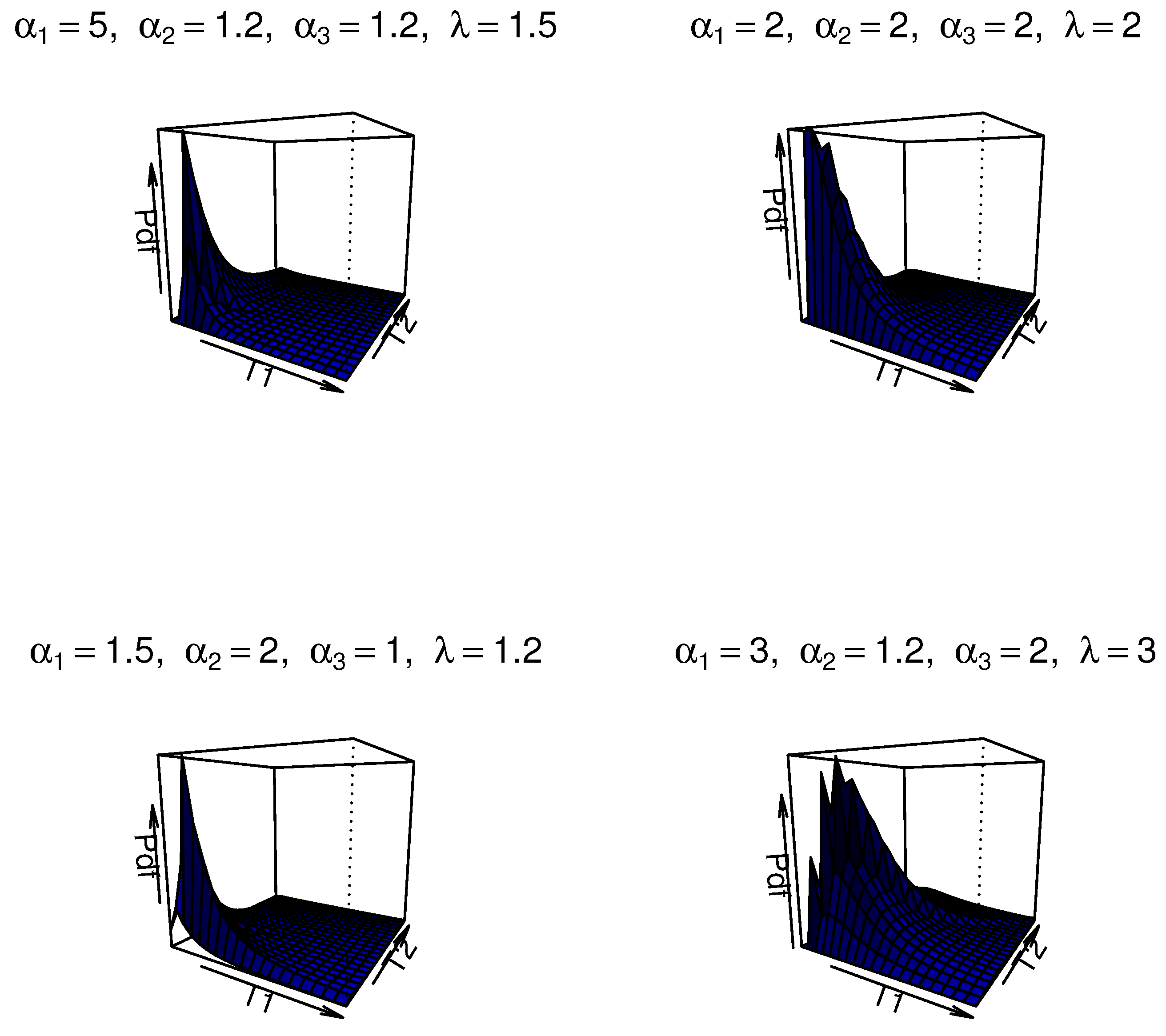
We illustrate the potential motivation and comparative advantages of this model for modeling dependent competing risks. Firstly, the MOBIEP distribution inherently captures nonlinear dependence structures between latent failure times via its shape and scale parameters. This characteristic is crucial in competing risk scenarios where failure modes may exhibit complex interactions. Secondly, the IEP model is well-suited for modeling extreme-value data or heavy-tailed survival patterns, which are prevalent in reliability and survival analyses. Thirdly, the closed-form survival function facilitates tractable likelihood construction, thereby enhancing computational feasibility for both classical and Bayesian frameworks. Additionally, this model possesses distinct advantages when compared with alternative distributions. We note that copulas allow for flexible dependency modeling; however, they often lack interpretability in competing risk contexts and may necessitate ad hoc assumptions for marginal distributions. The MOBIEP offers a unified parametric framework with direct interpretability of parameters. Similarly, traditional bivariate models such as Weibull/exponential bivariate distributions impose restrictive assumptions (e.g., monotonic hazard rates) and symmetric dependencies, whereas the MOBIEP accommodates asymmetric dependence and nonmonotonic hazards. For ilustration, some plots of the density for the MOBIEP model are provided in Figure 1.

Figure 1. The surface plots of the joint PDF of $T_1$ and $T_2$ with different values of $({\alpha }_1,{\alpha }_2,{\alpha }_3,\lambda )$.

2.2. Data Description

Assume that n units are tested under two dependent causes of failure. The lifetimes of the testing units are examined under two competing risks, $T_1$ and $T_2$, with $(T_1,T_2)\sim \mathrm{MOBIEP}({\alpha }_1,{\alpha }_2,{\alpha }_3,\lambda )$. Let $Y=\min (T_1,T_2)$ be the lifetime of the considered units. Thus, observations under complete sample can be expressed as

$$\begin{array}{c}\hfill \{(y_1,{\delta }_1),(y_2,{\delta }_2),\dots ,(y_n,{\delta }_n)\},\end{array}$$

(6)

with $y_i=\min (t_{1i},t_{2i})$. Here, $t_{ji},j=1,2,i=1,2,\dots ,n$ is the ith failure time of $T_j$. Further, the notation ${\delta }_i$ is the failure indicator, such that

$$\begin{array}{c}\hfill {\delta }_i=\left\{\begin{array}{cc}0,\hfill & \mathrm{if}{t}_{i1}=t_{i2};\hfill \\ 1,\hfill & \mathrm{if}{t}_{i1}<t_{i2};\hfill \\ 2,\hfill & \mathrm{if}{t}_{i1}>t_{i2};\hfill \\ 3,\hfill & \mathrm{if}\mathrm{failure}\mathrm{cause}\mathrm{not}\mathrm{known}.\hfill \end{array}\right.\end{array}$$

(7)

With the GPHC approach, the competing risk data are given by

$$\begin{array}{c}\hfill \left\{\begin{array}{cc}\mathrm{Case}\mathrm{I}:\left\{(y_{1:m:n},{\delta }_1,r_1),(y_{2:m:n},{\delta }_2,r_2),\dots ,(y_{k:m:n},{\delta }_k,r_k)\right\},\hfill & \mathrm{if}T<y_{k:m:n}<y_{m:m:n},\hfill \\ \mathrm{Case}\mathrm{II}:\left\{(y_{1:m:n},{\delta }_1,r_1),(y_{2:m:n},{\delta }_2,r_2),\dots ,(y_{d:m:n},{\delta }_d,r_d)\right\},\hfill & \mathrm{if}{y}_{k:m:n}<T<y_{m:m:n},\hfill \\ \mathrm{Case}\mathrm{III}:\left\{(y_{1:m:n},{\delta }_1,r_1),(y_{2:m:n},{\delta }_2,r_2),\dots ,(y_{m:m:n},{\delta }_m,r_m)\right\},\hfill & \mathrm{if}{y}_{k:m:n}<y_{m:m:n}<T.\hfill \end{array}\right.\end{array}$$

(8)

Here, $\left\{r_i:i=1,2,\dots ,m\right\}$ denotes the specified scheme in advance. Further, T is the monitoring time point and k is a given positive integer. Additionally, d indicates the failure items so that, in Case II, we have $y_{d:m:n}<y_{d+1:m:n}$.

Remark 1. 

In practical situations, identifying failure mechanisms presents a significant challenge; while advanced detection techniques can reveal various causes underlying different physical phenomena, complex internal structures and operating mechanisms often obscure precise identification. However, there are numerous instances where causes of failure cannot be appropriately identified. Therefore, it is observed from (7) that the assumption of partially identified causes of failure in competing risk data is more realistic and suitable for analyzing scenarios where complete knowledge of failure causes is unavailable.

For the sake of simplicity, the competing risk data given in (8) are rewritten as $\left\{(y_i,{\delta }_i,r_i):i=1,2,\dots ,m\right\}$ under the GPHC scenario, where $y_{i:m:n}$ is presented as $y_i$ for concision. Further, suppose the dependent causes of failure follow $\mathrm{MOBIEP}({\alpha }_1,{\alpha }_2,{\alpha }_3,\lambda )$; then, the likelihood can be expressed as

$$\begin{array}{cc}\hfill & L\left(data\right)\propto \hfill \\ \hfill & \left\{\begin{array}{c}\prod _{i=1}^k{\left[f_{(T_1,T_2)}(y_i,y_i)\right]}^{{\delta }_{i0}}{\left[-{\displaystyle \frac{\partial S_{(T_1,T_2)}(t_1,t_2)}{\partial t_1}}{|}_{(y_i,y_i)}\right]}^{{\delta }_{i1}}{\left[-{\displaystyle \frac{\partial S_{(T_1,T_2)}(t_1,t_2)}{\partial t_2}}{|}_{(y_i,y_i)}\right]}^{{\delta }_{i2}}\hfill \\ .{\left[f_{IEP}(y_i;\lambda ,{\alpha }_{123})\right]}^{{\delta }_{i3}}{\left[S_{(T_1,T_2)(y_i,y_i)}\right]}^{r_i}\hfill & \mathrm{Case}\mathrm{I}\hfill \\ \prod _{i=1}^d{\left[f_{(T_1,T_2)}(y_i,y_i)\right]}^{{\delta }_{i0}}{\left[-{\displaystyle \frac{\partial S_{(T_1,T_2)}(t_1,t_2)}{\partial t_1}}{|}_{(y_i,y_i)}\right]}^{{\delta }_{i1}}{\left[-{\displaystyle \frac{\partial S_{(T_1,T_2)}(t_1,t_2)}{\partial t_2}}{|}_{(y_i,y_i)}\right]}^{{\delta }_{i2}}\hfill \\ .{\left[f_{IEP}(y_i;\lambda ,{\alpha }_{123})\right]}^{{\delta }_{i3}}{\left[S_{(T_1,T_2)(y_i,y_i)}\right]}^{r_i}{\left[S_{(T_1,T_2)}(T,T)\right]}^{r_{d+1}^{*}}\hfill & \mathrm{Case}\mathrm{II}\hfill \\ \prod _{i=1}^m{\left[f_{(T_1,T_2)}(y_i,y_i)\right]}^{{\delta }_{i0}}{\left[-{\displaystyle \frac{\partial S_{(T_1,T_2)}(t_1,t_2)}{\partial t_1}}{|}_{(y_i,y_i)}\right]}^{{\delta }_{i1}}{\left[-{\displaystyle \frac{\partial S_{(T_1,T_2)}(t_1,t_2)}{\partial t_2}}{|}_{(y_i,y_i)}\right]}^{{\delta }_{i2}}\hfill \\ .{\left[f_{IEP}(y_i;\lambda ,{\alpha }_{123})\right]}^{{\delta }_{i3}}{\left[S_{(T_1,T_2)(y_i,y_i)}\right]}^{r_i}\hfill & \mathrm{Case}\mathrm{III}\hfill \end{array}\right.\hfill \end{array}$$

(9)

where $r_k=n-{\sum }_{i=1}^{k-1}(r_i+1)-1$ in Case I, and $r_{d+1}^{*}=n-{\sum }_{i=1}^d(r_i+1)$ in Case II. The function ${\delta }_{ij}$ is written as

$${\delta }_{ij}=I_{({\delta }_i=j)}=\left\{\begin{array}{cc}1,\hfill & {\delta }_i=j;\hfill \\ 0,\hfill & {\delta }_i\ne j,j=0,1,2,3.\hfill \end{array}\right.$$

For cause $j=0,1,2$, the data for the ith unit are completely known in the sense of failure time and related cause of failure. For $j=3$, the failure time is known; however, the cause of failure may not be detected, satisfying ${\sum }_{j=0}^3{\delta }_{ij}=1$ for all $i=1,2,\dots ,m$. For clarity, a brief explanation about how to establish Equation (9) is given. For data $(y_i,{\delta }_i)$ with ${\delta }_i=0$, the probability contribution of data $(y_i,{\delta }_i)$ at $t_1=t_2=y_i$ is constructed from Equation (7) as

$$\begin{array}{c}\hfill {\left[f_{(T_1,T_2)}(t_1,t_2)\right]}_{t_1=t_2=y_i}=f_{(T_1,T_2)}(y_i,y_i).\end{array}$$

For ${\delta }_i=1$, data $(y_i,{\delta }_i)$ are equivalent to event $\{y_i<T_1<y_i+d{y}_i,T_2>y_i\}$; then, the probability contribution can be obtained as

$$\begin{array}{c}\hfill \mathbb{P}(y_i<T_1<y_i+d{y}_i,T_2>y_i)=\left[-{\displaystyle \frac{\partial S_{(T_1,T_2)}(t_1,t_2)}{\partial t_1}}{|}_{(t_1,t_2)=(y_i,y_i)}\right]d{t}_i.\end{array}$$

For other cases of $(y_i,{\delta }_i)$ with ${\delta }_i=2$ and 3, the probability contributions could be obtained similarly. Then, the joint likelihood function of the GPHC competing risks data (8) can, respectively, be obtained under Cases I, II, and III.

Remark 2. 

Under the conditions where ${\delta }_{ij}=0$ and ${\delta }_{ij}=3$, it should be noted that the probabilities are similar; these are given by ${\displaystyle \frac{{\alpha }_3}{{\alpha }_{123}}}{f}_{IEP}(t;\lambda ,{\alpha }_{123})$ and $f_{IEP}(t;\lambda ,{\alpha }_{123})$, respectively. Additionally, failure times due to causes one and two are appropriately observed when ${\delta }_{ij}=0$. In the scenario where ${\delta }_{ij}=3$, although the failure time has been observed, the specific cause of the product failure remains unknown. Consequently, the cause of failure in this case is masked, and it can be regarded as the failure time of the variable $min(T_1,T_2)$, without a specified cause of failure. Consequently, the corresponding probability contribution is derived from the distribution of $min(T_1,T_2)$. Therefore, the coefficient ${\displaystyle \frac{{\alpha }_3}{{\alpha }_{123}}}$, which is omitted in the case where ${\delta }_{ij}=3$, may be considered as an additional factor provided by the cause of failure.

Based on Equation (9), let $\nu =({\alpha }_1,{\alpha }_2,{\alpha }_3,\lambda )$ with ${\nu }_j={\alpha }_j,j=1,2,3$ and ${\nu }_4=\lambda$. Then, the corresponding likelihood functions $L_1\left(\nu \right),L_2\left(\nu \right)$ and $L_3\left(\nu \right)$ of $\nu$ for the Cases I, II, and III, are further expressed as

$$\begin{array}{cc}\hfill L_1\left(\nu \right)& \propto \prod _{i=1}^k\lambda {\alpha }_1^{{\delta }_{i1}}{\alpha }_2^{{\delta }_{i2}}{\alpha }_3^{{\delta }_{i0}}{\alpha }_{123}^{{\delta }_{i3}}{y}_i^{\lambda -1}{(1+y_i)}^{-(\lambda +1)}{\left(1-a{\left(y_i\right)}^{-\lambda }\right)}^{{\alpha }_{123}(r_i+1)-1},\hfill \\ \hfill L_2\left(\nu \right)& \propto \prod _{i=1}^d\lambda {\alpha }_1^{{\delta }_{i1}}{\alpha }_2^{{\delta }_{i2}}{\alpha }_3^{{\delta }_{i0}}{\alpha }_{123}^{{\delta }_{i3}}{y}_i^{\lambda -1}{(1+y_i)}^{-(\lambda +1)}{\left(1-a{\left(y_i\right)}^{-\lambda }\right)}^{{\alpha }_{123}(r_i+1)-1}{\left(1-a{\left(T\right)}^{-\lambda }\right)}^{{\alpha }_{123}{r}_{d+1}^{*}},\hfill \\ \hfill L_3\left(\nu \right)& \propto \prod _{i=1}^m\lambda {\alpha }_1^{{\delta }_{i1}}{\alpha }_2^{{\delta }_{i2}}{\alpha }_3^{{\delta }_{i0}}{\alpha }_{123}^{{\delta }_{i3}}{y}_i^{\lambda -1}{(1+y_i)}^{-(\lambda +1)}{\left(1-a{\left(y_i\right)}^{-\lambda }\right)}^{{\alpha }_{123}(r_i+1)-1}.\hfill \end{array}$$

(10)

3. Classical Inference

In this section, we discuss MLEs of model parameters; subsequently, the asymptotic confidence intervals (ACIs) are obtained.

3.1. Maximum Likelihood Estimation

Due to the different expressions of the likelihood functions under the GPHC scenario, assumptions are made. Accordingly, the likelihood functions $L_1\left(\nu \right),L_2\left(\nu \right)$ and $L_3\left(\nu \right)$ can be rewritten in a single expression. Let $d^{*}$ be the observed failure number in Cases I, II, and III. Then, we have

$$d^{*}=\left\{\begin{array}{cc}k,\hfill & \mathrm{Case}\mathrm{I};\hfill \\ d,\hfill & \mathrm{Case}\mathrm{II};\hfill \\ m,\hfill & \mathrm{Case}\mathrm{III}.\hfill \end{array}\right.$$

The failure times data (Equation (7)) in each case are denoted by $l_1={\sum }_{i=1}^{d^{*}}{\delta }_{i1}$. Further, let $l_2={\sum }_{i=1}^{d^{*}}{\delta }_{i2}$, $l_3={\sum }_{i=1}^{d^{*}}{\delta }_{i0}$ and $l_0={\sum }_{i=1}^{d^{*}}{\delta }_{i3}$ satisfying $d^{*}={\sum }_{j=1}^3{l}_j$,

$${\Omega }_1\left(\lambda \right)=\left\{\begin{array}{cc}\sum _{i=1}^k(1+r_i)log\left(1-a{\left(y_i\right)}^{-\lambda }\right)\hfill & \mathrm{Case}\mathrm{I};\hfill \\ \sum _{i=1}^d(1+r_i)log\left(1-a{\left(y_i\right)}^{-\lambda }\right)+\left(r_{d+1}^{*}\right)log\left(1-a{\left(T\right)}^{-\lambda }\right)\hfill & \mathrm{Case}\mathrm{II};\hfill \\ \sum _{i=1}^m(1+r_i)log\left(1-a{\left(y_i\right)}^{-\lambda }\right)\hfill & \mathrm{Case}\mathrm{III},\hfill \end{array}\right.$$

and

$${\Omega }_2\left(\lambda \right)=\left\{\begin{array}{cc}\sum _{i=1}^{k}log\left(1-a{\left(y_i\right)}^{-\lambda }\right)\hfill & \mathrm{Case}\mathrm{I};\hfill \\ \sum _{i=1}^{d}log\left(1-a{\left(y_i\right)}^{-\lambda }\right)\hfill & \mathrm{Case}\mathrm{II};\hfill \\ \sum _{i=1}^{m}log\left(1-a{\left(y_i\right)}^{-\lambda }\right)\hfill & \mathrm{Case}\mathrm{III}.\hfill \end{array}\right.$$

Therefore, the likelihood function of ${\alpha }_1,{\alpha }_2,{\alpha }_3$, and $\lambda$, namely $L\left(\nu \right),$ is rewritten as

$$\begin{array}{c}\hfill L\left(\nu \right)={\lambda }^{d^{*}}{\alpha }_1^{l_1}{\alpha }_2^{l_2}{\alpha }_3^{l_3}{\alpha }_{123}^{l_0}{\left(\prod _{i=1}^{d^{*}}{y}_i\right)}^{(\lambda -1)}{\left(\prod _{i=1}^{d^{*}}\left(1+y_i\right)\right)}^{-(\lambda +1)}{e}^{{\alpha }_{123}{\Omega }_1\left(\lambda \right)-{\Omega }_2\left(\lambda \right)}\end{array}$$

(11)

and the associated log–likelihood function $l\left(\nu \right)$ is expressed as

$$\begin{array}{cc}\hfill l\left(\nu \right)& =d^{*}log\left(\lambda \right)+l_{1}log\left({\alpha }_1\right)+l_{2}log\left({\alpha }_2\right)+l_{3}log\left({\alpha }_3\right)+l_{0}log\left({\alpha }_{123}\right)+(\lambda -1)\sum _{i=1}^{d^{*}}log\left(y_i\right)\hfill \\ \hfill & -(\lambda +1)\sum _{i=1}^{d^{*}}log(1+y_i)+{\alpha }_{123}{\Omega }_1\left(\lambda \right)-{\Omega }_2\left(\lambda \right).\hfill \end{array}$$

(12)

The MLEs of ${\alpha }_1,{\alpha }_2,{\alpha }_3$, and $\lambda$ are presented as follows.

Theorem 2. 

Let GPHC competing risk data follow the MOBIEP $({\alpha }_1,{\alpha }_2,{\alpha }_3,\lambda )$ distribution. Then, for $l_j>0,j=1,2,3,$ the MLE of ${\alpha }_j$, given λ, is obtained as follows

$$\begin{array}{c}\hfill {\widehat{\alpha }}_j=-{\displaystyle \frac{l_j{d}^{*}}{l_{123}{\Omega }_1\left(\lambda \right)}}\mathit{with}{l}_{123}=l_1+l_2+l_3.\end{array}$$

Proof. 

See Appendix D.    □

Theorem 3. 

Let the GPHC competing risk data follow the MOBIEP $({\alpha }_1,{\alpha }_2,{\alpha }_3,\lambda )$ distribution. Then, for $l_j>0,j=1,2,3$, the MLE of λ uniquely exists as the solution of the following equation

$$\begin{array}{c}\hfill {\displaystyle \frac{d^{*}}{\lambda }}-d^{*}{\displaystyle \frac{{\Omega }_1^{\prime }\left(\lambda \right)}{{\Omega }_1\left(\lambda \right)}}-\sum _{i=1}^{d^{*}}{\displaystyle \frac{loga\left(y_i\right)}{\left(1-a{\left(y_i\right)}^{-\lambda }\right)}}=0,\end{array}$$

(13)

where

$${\Omega }_1^{\prime }\left(\lambda \right)=\left\{\begin{array}{cc}\sum _{i=1}^k(1+r_i){\displaystyle \frac{a{\left(y_i\right)}^{-\lambda }loga\left(y_i\right)}{(1-a{\left(y_i\right)}^{-\lambda })}},\hfill & \mathit{Case}I;\hfill \\ \\ \sum _{i=1}^d(1+r_i){\displaystyle \frac{a{\left(y_i\right)}^{-\lambda }loga\left(y_i\right)}{1-a{\left(y_i\right)}^{-\lambda }}}+\left(r_{d+1}^{*}\right){\displaystyle \frac{a{\left(T\right)}^{-\lambda }loga\left(T\right)}{(1-a{\left(T\right)}^{-\lambda })}},\hfill & \mathit{Case}\mathit{II};\hfill \\ \\ \sum _{i=1}^m(1+r_i){\displaystyle \frac{a{\left(y_i\right)}^{-\lambda }loga\left(y_i\right)}{(1-a{\left(y_i\right)}^{-\lambda })}},\hfill & \mathit{Case}\mathit{III}.\hfill \end{array}\right.$$

Proof. 

See Appendix E.    □

Since the explicit form of the estimator $\widehat{\lambda }$ of $\lambda$ does not exist, the required estimate can be obtained using the fixed-point iteration technique. Additionally, the MLEs of ${\alpha }_1$, ${\alpha }_2$, and ${\alpha }_3$ can be obtained from Theorem 2, as follows:

$$\begin{array}{c}\hfill {\widehat{\alpha }}_1=-{\displaystyle \frac{l_1{d}^{*}}{l_{123}{\Omega }_1\left(\widehat{\lambda }\right)}},{\widehat{\alpha }}_2=-{\displaystyle \frac{l_2{d}^{*}}{l_{123}{\Omega }_1\left(\widehat{\lambda }\right)}}\mathrm{and}{\widehat{\alpha }}_3=-{\displaystyle \frac{l_3{d}^{*}}{l_{123}{\Omega }_1\left(\widehat{\lambda }\right)}}.\end{array}$$

3.2. Approximate Confidence Intervals

The observed Fisher information for $\nu ={({\alpha }_1,{\alpha }_2,{\alpha }_3,\lambda )}^{\prime }$ is given by

$$\begin{array}{cc}\hfill I\left(\nu \right)& ={\left[I_{ij}\right]}_{i,j=1,2,3,4}={\left[-{\displaystyle \frac{{\partial }^{2}l\left(\nu \right)}{\partial {\nu }_i\partial {\nu }_j}}\right]}_{i,j=1,2,3,4}^{\nu =\widehat{\nu }}\hfill \\ \hfill & ={\left(\begin{array}{cccc}-{\displaystyle \frac{{\partial }^{2}l}{\partial {\alpha }_1^2}}& -{\displaystyle \frac{{\partial }^{2}l}{\partial {\alpha }_1\partial {\alpha }_2}}& -{\displaystyle \frac{{\partial }^{2}l}{\partial {\alpha }_1\partial {\alpha }_3}}& -{\displaystyle \frac{{\partial }^{2}l}{\partial {\alpha }_1\partial \lambda }}\\ -{\displaystyle \frac{{\partial }^{2}l}{\partial {\alpha }_2\partial {\alpha }_1}}& -{\displaystyle \frac{{\partial }^{2}l}{\partial {\alpha }_2^2}}& -{\displaystyle \frac{{\partial }^{2}l}{\partial {\alpha }_2\partial {\alpha }_3}}& -{\displaystyle \frac{{\partial }^{3}l}{\partial {\alpha }_2\partial \lambda }}\\ -{\displaystyle \frac{{\partial }^{3}l}{\partial {\alpha }_3\partial {\alpha }_1}}& -{\displaystyle \frac{{\partial }^{3}l}{\partial {\alpha }_3\partial {\alpha }_2}}& -{\displaystyle \frac{{\partial }^{3}l}{\partial {\alpha }_3\partial {\alpha }_3}}& -{\displaystyle \frac{{\partial }^{2}l}{\partial {\alpha }_3\partial \lambda }}\\ -{\displaystyle \frac{{\partial }^{2}l}{\partial \lambda \partial {\alpha }_1}}& -{\displaystyle \frac{{\partial }^{2}l}{\partial \lambda \partial {\alpha }_2}}& -{\displaystyle \frac{{\partial }^{2}l}{\partial \lambda \partial {\alpha }_3}}& -{\displaystyle \frac{{\partial }^{2}l}{\partial {\lambda }^2}}\end{array}\right)}_{\nu =\widehat{\nu }},\hfill \end{array}$$

where the associated elements are obtained by direct computation. The detailed expressions are omitted here for the sake of concision.

Under mild regularity conditions, the approximate distribution of MLE $\widehat{\nu }$ is such that $\widehat{\nu }-\nu \stackrel{d}{\to }N(0,I^{-1}\left(\widehat{\nu }\right))$, where the notation “$\stackrel{d}{\to }$” means “convergence in distribution”, and $I^{-1}\left(\widehat{\nu }\right)$ represents the inverse of the observed Fisher information matrix, given below as

$$\begin{array}{c}\hfill I^{-1}\left(\widehat{\nu }\right)=\left(\begin{array}{cccc}Var({\widehat{\alpha }}_1,{\widehat{\alpha }}_1)& Cov({\widehat{\alpha }}_1,{\widehat{\alpha }}_2)& Cov({\widehat{\alpha }}_1,{\widehat{\alpha }}_3)& Cov({\widehat{\alpha }}_1,\widehat{\lambda })\\ Cov({\widehat{\alpha }}_2,{\widehat{\alpha }}_1)& Var({\widehat{\alpha }}_2,{\widehat{\alpha }}_2)& Cov({\widehat{\alpha }}_2,{\widehat{\alpha }}_3)& Cov({\widehat{\alpha }}_2,\widehat{\lambda })\\ Cov({\widehat{\alpha }}_3,{\widehat{\alpha }}_1)& Cov({\widehat{\alpha }}_3,{\widehat{\alpha }}_2)& Var({\widehat{\alpha }}_3,{\widehat{\alpha }}_3)& Cov({\widehat{\alpha }}_3,\widehat{\lambda })\\ Cov(\widehat{\lambda },{\widehat{\alpha }}_1)& Cov(\widehat{\lambda },{\widehat{\alpha }}_2)& Cov(\widehat{\lambda },{\widehat{\alpha }}_3)& Var(\widehat{\lambda },\widehat{\lambda })\end{array}\right).\end{array}$$

Now, for some $0<\gamma <1$, a $100(1-\gamma )\%$ confidence interval of ${\nu }_j,j=1,2,3,4,$ is obtained as

$$\begin{array}{c}\hfill \left(\widehat{{\nu }_j}-z_{\gamma /2}\sqrt{Var\left(\widehat{{\nu }_j}\right)},\widehat{{\nu }_j}+z_{\gamma /2}\sqrt{Var\left(\widehat{{\nu }_j}\right)}\right),j=1,2,3,4,\end{array}$$

where $z_{\gamma }$ is the $100\gamma \%$ percentile of standard normal distribution. Sometimes, these interval estimates may occasionally yield negative lower bounds. In this regard, the delta method can be applied to derive the distribution of $log\left(\widehat{{\nu }_j}\right),j=1,2,3,4$, such as ${\displaystyle \frac{log{\widehat{\nu }}_j-log{\nu }_j}{\sqrt{Var(log{\widehat{\nu }}_j)}}}\to \mathrm{N}(0,1),j=1,2,3,4$. Therefore, the desired interval of ${\nu }_j,j=1,2,3,4$ is obtained as

$$\begin{array}{c}\hfill \left({\displaystyle \frac{{\widehat{\nu }}_j}{exp\left\{z_{\gamma /2}\sqrt{\widehat{Var}(log{\widehat{\nu }}_j)}\right\}}},\widehat{{\nu }_j}exp\left\{z_{\gamma /2}\sqrt{\widehat{Var}(log{\widehat{\nu }}_j)}\right\}\right),j=1,2,3,4,\end{array}$$

where $\sqrt{\widehat{Var}(log{\widehat{\nu }}_j)}=Var\left({\widehat{\nu }}_j\right)/{{\widehat{\nu }}_j}^2,j=1,2,3,4$.

4. Bayesian Analysis

In data analysis, the Bayesian approach has gained considerable attention due to its capability to incorporate prior information. This feature is particularly valuable in various fields, such as bio-assay experiments, clinical trials, and competing risk models. This section presents Bayesian estimation using a general flexible prior. Accordingly, estimates of parameters and highest posterior density (HPD) credible intervals are obtained.

4.1. Prior Information

Following the idea of Pena and Gupta [15], a general flexible prior for model parameters is constructed as follows. Assuming ${\alpha }_{123}={\alpha }_1+{\alpha }_2+{\alpha }_3,$ a gamma prior ${\pi }_0\left({\alpha }_{123}\right|a_0,b_0)$ for ${\alpha }_{123}$ is presented, as follows:

$$\begin{array}{c}\hfill {\pi }_0\left({\alpha }_{123}\right|a_0,b_0)={\displaystyle \frac{b_0^{a_0}}{\Gamma \left(a_0\right)}}{\alpha }_{123}^{a_0-1}{e}^{-b_0{\alpha }_{123}},a_0>0,b_0>0,{\alpha }_{123}>0.\end{array}$$

Now, given ${\alpha }_{123}$, $({\displaystyle \frac{{\alpha }_1}{{\alpha }_{123}}},{\displaystyle \frac{{\alpha }_2}{{\alpha }_{123}}})$ has the following prior, with density

$$\begin{array}{cc}\hfill {\pi }_1\left({\displaystyle \frac{{\alpha }_1}{{\alpha }_{123}}},{\displaystyle \frac{{\alpha }_2}{{\alpha }_{123}}}|{\alpha }_{123},c_1,c_2,c_3\right)& ={\displaystyle \frac{\Gamma (c_1+c_2+c_3)}{\Gamma \left(c_1\right)\Gamma \left(c_2\right)\Gamma \left(c_3\right)}}{\left({\displaystyle \frac{{\alpha }_1}{{\alpha }_{123}}}\right)}^{c_1-1}\hfill \\ \hfill & ·{\left({\displaystyle \frac{{\alpha }_2}{{\alpha }_{123}}}\right)}^{c_2-1}{\left({\displaystyle \frac{{\alpha }_3}{{\alpha }_{123}}}\right)}^{c_3-1},c_1>0,c_2>0,c_3>0.\hfill \end{array}$$

(14)

Therefore, the prior of $({\alpha }_1,{\alpha }_2,{\alpha }_3)$, namely $\pi ({\alpha }_1,{\alpha }_2,{\alpha }_3|a_0,b_0,c_1,c_2,c_3),$ is given by

$$\begin{array}{cc}\hfill \pi \left({\alpha }_1,{\alpha }_2,{\alpha }_3|a_0,b_0,c_1,c_2,c_3\right)& ={\displaystyle \frac{\Gamma (c_1+c_2+c_3)}{\Gamma \left(a_0\right)}}{\displaystyle \frac{b_0^{a_0-c_1-c_2-c_3}}{{\left({\alpha }_{123}\right)}^{c_1+c_2+c_3-a_0}}}·{\displaystyle \frac{b_0^{c_3}}{\Gamma \left(c_3\right)}}{\alpha }_3^{c_3-1}{e}^{-b_0{\alpha }_3}\hfill \\ \hfill & ·{\displaystyle \frac{b_0^{c_1}}{\Gamma \left(c_1\right)}}{\alpha }_1^{c_1-1}{e}^{-b_0{\alpha }_1}·{\displaystyle \frac{b_0^{c_2}}{\Gamma \left(c_2\right)}}{\alpha }_2^{c_2-1}{e}^{-b_0{\alpha }_2},\hfill \end{array}$$

(15)

where $c_{123}=c_1+c_2+c_3$. The prior (15) is referred to the Gamma–Dirichlet prior, denoted by $\mathrm{GD}(a_0,b_0,c_1,c_2,c_3)$. This family of priors offers a very flexible approach for Bayesian computation.

In addition, suppose that parameter $\lambda$ has an independent gamma prior

$$\begin{array}{c}\hfill \pi \left(\lambda \right|a_1,b_1)={\displaystyle \frac{b_1^{a_1}}{\Gamma \left(a_1\right)}}{\lambda }^{a_1-1}{e}^{-b_1\lambda },a_1>0,b_1>0.\end{array}$$

(16)

Finally, the joint prior distribution of ${\alpha }_1,{\alpha }_2,{\alpha }_3$ and $\lambda ,$ turns out to be

$$\begin{array}{c}\hfill \pi ({\alpha }_1,{\alpha }_2,{\alpha }_3,\lambda )=\pi \left(\lambda \right|a_1,b_1)\pi \left({\alpha }_1,{\alpha }_2,{\alpha }_3|a_0,b_0,c_1,c_2,c_3\right)\end{array}$$

(17)

and, accordingly, the posterior density is obtained as follows:

$$\begin{array}{c}\hfill \pi \left({\alpha }_1,{\alpha }_2,{\alpha }_3,\lambda |data\right)={\displaystyle \frac{\pi ({\alpha }_1,{\alpha }_2,{\alpha }_3,\lambda )L\left(\nu \right)}{{\oint }_4\pi ({\alpha }_1,{\alpha }_2,{\alpha }_3,\lambda )L\left(\nu \right)}},\end{array}$$

(18)

where ${\oint }_4(.)d\nu ={\int }_0^{\infty }{\int }_0^{\infty }{\int }_0^{\infty }{\int }_0^{\infty }(.)d{\alpha }_{1}d{\alpha }_2{\alpha }_{3}d\lambda$.

For arbitrary parametric function $\eta ({\alpha }_1,{\alpha }_2,{\alpha }_3,\lambda )$, the corresponding Bayes estimator $\widehat{\eta }({\alpha }_1,{\alpha }_2,{\alpha }_3,\lambda )$ under the squared error loss is obtained as

$$\begin{array}{c}\hfill \widehat{\eta }({\alpha }_1,{\alpha }_2,{\alpha }_3,\lambda )={\displaystyle \frac{{\oint }_4\eta ({\alpha }_1,{\alpha }_2,{\alpha }_3,\lambda )\pi ({\alpha }_1,{\alpha }_2,{\alpha }_3,\lambda )L\left(\nu \right)d\nu }{{\oint }_4\pi ({\alpha }_1,{\alpha }_2,{\alpha }_3,\lambda )L\left(\nu \right)d\nu }}.\end{array}$$

(19)

Clearly, there is no closed form for this Bayes estimator. Therefore, a Monte Carlo sampling method is implemented to compute this estimate.

4.2. Posterior Analysis and Importance Sampling

The posterior density (18) of the parameters ${\alpha }_1,{\alpha }_2,{\alpha }_3$, and $\lambda$ can be rewritten as

$$\begin{array}{c}\hfill \pi ({\alpha }_1,{\alpha }_2,{\alpha }_3,\lambda |data)=M\left(\lambda \right){\pi }^{*}({\alpha }_1,{\alpha }_2,{\alpha }_3|\lambda ,data){\pi }^{*}\left(\lambda \right|data),\end{array}$$

(20)

where

$$\begin{array}{cc}\hfill {\pi }^{*}\left(\lambda \right|data)& =\mathrm{Gamma}\left(d^{*}+a_1,b_1+\sum _{i=1}^{d^{*}}loga\left(y_i\right)\right),\hfill \\ \hfill {\pi }^{*}({\alpha }_1,{\alpha }_2,{\alpha }_3|\lambda )& =\mathrm{GD}(d^{*}+a_0,b_0-{\Omega }_1\left(\lambda \right),l_1+c_1,l_2+c_2,l_3+c_3),\hfill \end{array}$$

(21)

and

$$\begin{array}{c}\hfill M\left(\lambda \right)={\displaystyle \frac{e^{-{\Omega }_2\left(\lambda \right)}}{{\left[b_0-{\Omega }_1\left(\lambda \right)\right]}^{a_0+d^{*}}}},\end{array}$$

with notation $Gamma(·,·)$ denting the gamma distribution. So, the estimator of $\eta ({\alpha }_1,{\alpha }_2,{\alpha }_3,\lambda )$ in (19) is rewritten as

$$\begin{array}{c}\hfill \widehat{\eta }={\displaystyle \frac{{\oint }_4\eta ({\alpha }_1,{\alpha }_2,{\alpha }_3,\lambda )M\left(\lambda \right){\pi }^{*}({\alpha }_1,{\alpha }_2,{\alpha }_3|\lambda ,data){\pi }^{*}\left(\lambda \right|data)L\left(\nu \right)d\nu }{{\oint }_{4}M\left(\lambda \right){\pi }^{*}({\alpha }_1,{\alpha }_2,{\alpha }_3|\lambda ,data){\pi }^{*}\left(\lambda \right|data)L\left(\nu \right)d\nu }}.\end{array}$$

(22)

We now employ the following sampling technique to compute the point and HPD-credible interval estimates of $\eta$ under the GPHC scheme. The associated computational procedure is given as follows (see Algorithm 1).    

Algorithm 1: Bayesian importance sampling.

Step 1  Obtain a sample for $\lambda$ using $\mathrm{Gamma}(d^{*}+a_1,b_1+{\sum }_{i=1}^{d^{*}}loga\left(y_i\right))$. Step 2  For given $\lambda$, obtain samples for $({\alpha }_1,{\alpha }_2,{\alpha }_3)$ from $\mathrm{GD}\left(d^{*}+a_0,b_0-{\Omega }_1\left(\lambda \right),l_1+c_1,l_2+c_2,l_3+c_3\right)$. Step 3  Previous steps are repeated N times to obtain samples $\{\left({\alpha }_1^s,{\alpha }_2^s,{\alpha }_3^s,{\lambda }^s\right),s=1,2,\dots ,N\}$ for $({\alpha }_1,{\alpha }_2,{\alpha }_3,\lambda )$. Step 4  The required Bayes estimate of $\eta ({\alpha }_1,{\alpha }_2,{\alpha }_3,\lambda )$ is now computed as $$\begin{array}{c}\hfill \widehat{\eta }({\alpha }_1,{\alpha }_2,{\alpha }_3,\lambda )={\displaystyle \frac{{\sum }_{l=N_0+1}^N\eta ({\alpha }_1^s,{\alpha }_2^s,{\alpha }_3^s,{\lambda }^s)M({\alpha }_1^s,{\alpha }_2^s,{\alpha }_3^s,{\lambda }^s)}{{\sum }_{l=N_0+1}^{N}M({\alpha }_1^s,{\alpha }_2^s,{\alpha }_3^s,{\lambda }^s)}}.\end{array}$$ Step 5  For interval construction, arrange all estimates $\eta ({\alpha }_1^s,{\alpha }_2^s,{\alpha }_3^s,{\lambda }^s),s=N_0+1,N_0+2,\dots ,N$ in an ascending order as ${\eta }^{\left[1\right]},{\eta }^{\left[2\right]},\dots ,{\eta }^{[N-N_0]}.$ A series of $100(1-\gamma )$ credible intervals of $\eta$ is given by $$\begin{array}{c}\hfill \left({\eta }^{\left[s\right]},{\eta }^{[s+N-N_0-\left[\gamma (N-N_0+1)\right]]}\right),s=1,2,\dots ,\left[(N-N_0)\gamma \right],\end{array}$$ where $[·]$ denotes the greatest integer function. In sequel, the HPD interval of $\eta ({\alpha }_1,{\alpha }_2,{\alpha }_3,\lambda )$ is the $s^{*}$th one, satisfying $$\begin{array}{c}\hfill {\eta }^{[s^{*}+N-N_0-[\gamma (N-N_0)+1]]}-{\eta }^{\left[s^{*}\right]}=\underset{s=1}{\overset{(N-N_0)\gamma }{min}}\left({\eta }^{[s+N-N_0-[\gamma (N-N_0)+1]]}-{\eta }^{\left[s\right]}\right).\end{array}$$

5. Simulation Study

In this section, extensive simulation experiments are conducted to assess the performances of the proposed estimates. Additionally, a real-life dataset is discussed to demonstrate practical application.

5.1. Simulation Results

In this part, a simulation analysis is carried out to evaluate the performance of the proposed methods under the GPHC competing risk data. For various sample sizes $(n,m)$, censoring schemes ($r_1,r_2,\dots ,r_m$), and monitoring points $(T,k)$, the point estimates of parameters ${\alpha }_1$, ${\alpha }_2$, ${\alpha }_3$, and $\lambda$ are evaluated using average bias (AB) and mean squared error (MSE) values. The interval estimates are evaluated based on the average length (AL) and the coverage probabilities (CPs).

The GPHC competing risk data are obtained as follows: First, a progressively censored sample for the jth $(j=1,2)$ cause is generated by using the algorithm of Balakrishnan and Sandhu [26] based on IEP model with parameters $\lambda$ and ${\alpha }_j+{\alpha }_3$. These two sets of samples are compared with respect to $(T,k)$ to obtain the GPHC competing risk data along with the associated causes of failure. Finally, these competing risk data are masked with probability, p, to obtain partially observed GPHC competing risk data. It is noted that a group of iid random data containing either 0 or 1 is generated using Bernoulli trials with probability, p, where the sample size is equal to that of the competing risk data. If a Bernoulli trial yields zero, the cause of failure is considered as unknown. Conversely, if one appears, the cause of failure is considered to be detected.

In the simulated illustration, we randomly select parameter (${\alpha }_1$, ${\alpha }_2$, ${\alpha }_3$, $\lambda$) as $(1.2,1.4,1.0,2.0)$. For the sake of convenience, a traditional Type-II censoring scheme is used with $r_1=\cdots =r_{m-1}=0$ and $r_m=n-m$. Furthermore, for the Bayes estimates, both non-informative priors (NIPs) with hyper-parameters $a_0=b_0=c_1=c_2=c_3=a_1=b_1=0.001$ and the informative prior (IP) with hyper-parameters $a_0=7.2,b_0=2,c_1=2.4,c_2=2.8,c_3=2,a_1=4,b_1=2$ are employed. Various estimates were obtained by considering 3000 replications. The computed results are presented in Table 1, Table 2, Table 3 and Table 4, where the interval estimates are computed with significance level $\gamma =0.05$.

Table 1. ABs and MSEs (within bracket) for OBIEP parameters when $T=1.5$.

$\mathit{p}=0.1$
$(\mathit{n},\mathit{m})$	$\mathit{k}$	MLE				IP Bayes				NIP Bayes
		${\mathit{\alpha }}_{\mathbf{1}}$	${\mathit{\alpha }}_{\mathbf{2}}$	${\mathit{\alpha }}_{\mathbf{3}}$	$\mathit{\lambda }$	${\mathit{\alpha }}_{\mathbf{1}}$	${\mathit{\alpha }}_{\mathbf{2}}$	${\mathit{\alpha }}_{\mathbf{3}}$	$\mathit{\lambda }$	${\mathit{\alpha }}_{\mathbf{1}}$	${\mathit{\alpha }}_{\mathbf{2}}$	${\mathit{\alpha }}_{\mathbf{3}}$	$\mathit{\lambda }$
(40, 30)	20	−0.2685	−0.3042	−0.2217	−0.2083	−0.0798	−0.0877	−0.0475	0.0798	−0.0877	−0.0938	−0.0546	0.0961
		0.2351	0.3473	0.1902	0.1513	0.1203	0.1693	0.1122	0.1224	0.1344	0.1749	0.1751	0.1305
	25	−0.2603	−0.2992	−0.2167	−0.1928	−0.0795	−0.0834	−0.0455	0.0951	−0.0847	−0.0914	−0.0536	0.0916
		0.2347	0.3142	0.1872	0.1484	0.1186	0.1535	0.0998	0.1172	0.1277	0.1620	0.1726	0.1213
(50, 35)	25	−0.2426	−0.2896	−0.2094	−0.1805	−0.0677	−0.0794	−0.0426	0.0896	−0.0744	−0.0908	−0.0507	0.0898
		0.2255	0.2730	0.1795	0.1405	0.1076	0.1486	0.0909	0.1159	0.1121	0.1578	0.1664	0.1171
	30	−0.2480	−0.2822	−0.2075	−0.1761	−0.0639	−0.0694	−0.0417	0.0878	−0.0721	−0.0882	−0.0491	0.0890
		0.2273	0.2665	0.1652	0.1354	0.1062	0.1440	0.0902	0.1083	0.1091	0.1579	0.1563	0.1096
(60, 40)	30	−0.2231	−0.2735	−0.2028	−0.1742	−0.0631	−0.0661	−0.0390	0.0828	−0.0719	−0.0861	−0.0459	0.0874
		0.2036	0.2612	0.1589	0.1352	0.0993	0.1423	0.0901	0.1041	0.1032	0.1511	0.1525	0.1035
	35	−0.2164	−0.2873	−0.1984	−0.1703	−0.0618	−0.0604	−0.0381	0.0752	−0.0708	−0.0859	−0.0448	0.0763
		0.1961	0.2563	0.1487	0.1306	0.0923	0.1420	0.0891	0.1037	0.0994	0.1489	0.1442	0.1042
(80, 60)	40	−0.2096	−0.2741	−0.1909	−0.1563	−0.0585	−0.0539	−0.0362	0.0743	−0.0658	−0.0794	−0.0397	0.0722
		0.1719	0.2277	0.1274	0.1264	0.0857	0.1391	0.0811	0.1007	0.0967	0.1479	0.1189	0.1013
	50	−0.2026	−0.2541	−0.1863	−0.1469	−0.0532	−0.0525	−0.0335	0.0738	−0.0596	−0.0749	−0.0352	0.0742
		0.1610	0.2083	0.1191	0.1190	0.0793	0.1203	0.0786	0.0880	0.0862	0.1358	0.1067	0.0919
$\mathit{p}=\mathbf{0.05}$
(40, 30)	20	−0.2615	−0.3306	−0.2247	−0.1795	−0.0744	−0.0882	−0.0461	0.0791	−0.0802	−0.0959	−0.0532	0.0955
		0.2262	0.3009	0.1823	0.1492	0.1190	0.1530	0.1014	0.1189	0.1325	0.1703	0.1751	0.1349
	25	−0.2505	−0.2848	−0.2098	−0.1695	−0.0647	−0.0723	−0.0460	0.0779	−0.0799	0.0927	0.0497	0.0948
		0.2196	0.2911	0.1816	0.1401	0.1157	0.1493	0.0941	0.1116	0.1302	0.1697	0.1743	0.1322
(50, 35)	25	−0.2495	−0.2847	−0.2062	−0.1583	−0.0592	−0.0622	−0.0449	0.0759	−0.0796	−0.0922	−0.0481	0.0943
		0.2186	0.2829	0.1613	0.1338	0.1143	0.1358	0.0926	0.1082	0.1272	0.1683	0.1717	0.1246
	30	−0.2485	−0.2784	−0.1952	−0.1446	−0.0504	−0.0615	−0.0445	0.0722	−0.0601	−0.0915	−0.0466	0.0924
		0.2151	0.2812	0.1574	0.1323	0.1135	0.1333	0.0974	0.1058	0.1191	0.1659	0.1686	0.1181
(60, 40)	30	−0.2337	−0.2681	−0.1924	−0.1435	−0.0509	−0.0612	−0.0421	0.0697	−0.0748	−0.0909	−0.0443	0.0914
		0.1925	0.2712	0.1473	0.1303	0.1056	0.1286	0.0938	0.1035	0.1166	0.1605	0.1607	0.1134
	35	−0.2318	−0.2581	−0.1838	−0.1369	−0.0507	−0.0594	−0.0414	0.0635	−0.0705	−0.0855	−0.0397	0.0893
		0.1893	0.2596	0.1381	0.1258	0.1045	0.1144	0.0850	0.1021	0.1091	0.1592	0.1392	0.1097
(80, 60)	40	−0.2266	−0.2567	−0.1767	−0.1287	−0.0492	−0.0588	−0.0403	0.0624	−0.0699	−0.0803	−0.0365	0.0846
		0.1723	0.2284	0.1208	0.1224	0.1027	0.1097	0.0784	0.0933	0.1076	0.1583	0.1108	0.1051
	50	−0.2116	−0.2427	−0.1671	−0.1122	−0.0494	−0.0464	−0.0392	0.0594	−0.0675	−0.0797	−0.0295	0.0836
		0.1667	0.2102	0.1195	0.1219	0.1002	0.1091	0.0771	0.0911	0.1068	0.1554	0.1095	0.1029

Table 2. ABs and MSEs (within bracket) for OBIEP parameters when $T=2$.

$\mathit{p}=0.1$
$(\mathit{n},\mathit{m})$	$\mathit{k}$	MLE				IP Bayes				NIP Bayes
		${\mathit{\alpha }}_{\mathbf{1}}$	${\mathit{\alpha }}_{\mathbf{2}}$	${\mathit{\alpha }}_{\mathbf{3}}$	$\mathit{\lambda }$	${\mathit{\alpha }}_{\mathbf{1}}$	${\mathit{\alpha }}_{\mathbf{2}}$	${\mathit{\alpha }}_{\mathbf{3}}$	$\mathit{\lambda }$	${\mathit{\alpha }}_{\mathbf{1}}$	${\mathit{\alpha }}_{\mathbf{2}}$	${\mathit{\alpha }}_{\mathbf{3}}$	$\mathit{\lambda }$
(40, 30)	20	−0.2505	−0.3020	−0.1899	−0.1641	−0.0548	−0.0831	−0.0514	0.0784	−0.0790	−0.0946	0.0495	0.0975
		0.2109	0.2917	0.1765	0.1508	0.1194	0.1521	0.1017	0.1196	0.1361	0.1594	0.1533	0.1292
	25	−0.2241	−0.2877	−0.1784	−0.1569	−0.0493	−0.0821	−0.0456	0.0747	0.0759	−0.0928	0.0464	0.0932
		0.2069	0.2781	0.1663	0.1419	0.1104	0.1454	0.0982	0.1193	0.1304	0.1591	0.1465	0.1241
(50, 35)	25	−0.2149	−0.2806	−0.1667	−0.1525	−0.0477	−0.0789	−0.0553	0.0684	−0.0525	−0.0881	−0.0382	0.0897
		0.2057	0.2693	0.1579	0.1382	0.1015	0.1409	0.0849	0.1163	0.1288	0.1402	0.1386	0.1115
	30	−0.2136	−0.2743	−0.1524	−0.1514	−0.0452	−0.0688	−0.0546	0.0649	−0.0548	−0.0761	−0.0352	0.0838
		0.2054	0.2692	0.1576	0.1313	0.1336	0.1328	0.0831	0.1129	0.1378	0.1401	0.1274	0.1087
(60, 40)	30	−0.2063	−0.2686	−0.1449	−0.1452	−0.0447	−0.0637	−0.0516	0.0627	−0.0533	−0.0701	−0.0325	0.0833
		0.1839	0.2462	0.1491	0.1295	0.0998	0.1313	0.0822	0.1086	0.1281	0.1381	0.1213	0.0922
	35	−0.2051	−0.2502	−0.1427	−0.1323	−0.0438	−0.0621	−0.0515	0.0617	−0.0499	−0.0697	−0.0293	0.0807
		0.1920	0.2405	0.1392	0.1298	0.0987	0.1297	0.0818	0.1058	0.1373	0.1361	0.1196	0.0818
(80, 60)	40	−0.2412	−0.3273	−0.1402	−0.1328	−0.0425	−0.0608	−0.0511	0.0585	−0.0489	−0.0680	−0.0231	0.0775
		0.1626	0.1884	0.1208	0.1216	0.0983	0.1099	0.0765	0.1026	0.1326	0.1352	0.1178	0.0819
	50	−0.1953	−0.2352	−0.1386	−0.1267	−0.0398	−0.0608	−0.0496	0.0559	−0.0445	−0.0842	−0.0219	0.0723
		0.1561	0.1846	0.1149	0.1208	0.0884	0.1018	0.0671	0.1006	0.1302	0.1328	0.1125	0.0794
$\mathit{p}=\mathbf{0.05}$
(40, 30)	20	−0.2480	−0.3020	−0.2149	−0.1580	−0.0592	−0.0603	0.0631	−0.0699	−0.0607	−0.0842	0.0428	−0.0819
		0.2178	0.2753	0.1639	0.1449	0.1125	0.1382	0.1007	0.1159	0.3076	0.1583	0.1548	0.1114
	25	−0.2496	−0.2886	−0.2097	−0.1497	−0.0548	−0.0599	−0.0598	0.0678	0.0603	0.0781	−0.0421	0.0806
		0.2065	0.2593	0.1579	0.1427	0.1048	0.1255	0.0951	0.1105	0.3624	0.1482	0.1416	0.1098
(50, 35)	25	−0.2361	−0.2856	−0.2033	−0.1467	−0.0511	−0.0556	−0.0561	0.2161	−0.0534	−0.0682	−0.0408	0.0768
		0.1999	0.2654	0.1436	0.1304	0.0991	0.1208	0.0854	0.1093	0.2788	0.1444	0.1398	0.1041
	30	−0.2207	−0.2706	−0.1933	−0.1364	−0.0501	−0.0503	−0.0491	0.0542	−0.0458	−0.0681	−0.0404	0.0732
		0.1984	0.2589	0.1396	0.1243	0.0903	0.1207	0.0787	0.1074	0.2341	0.1393	0.1271	0.1031
(60, 40)	30	−0.2105	−0.2689	−0.1813	−0.1323	−0.0459	−0.0419	−0.0476	0.0498	−0.0449	−0.0520	−0.0396	0.0722
		0.1878	0.2490	0.1344	0.1295	0.0863	0.1181	0.0709	0.1051	0.1869	0.1267	0.1257	0.0957
	35	−0.2043	−0.2549	−0.1753	−0.1306	−0.0453	−0.0451	−0.0925	0.0436	−0.0437	−0.0527	−0.0373	0.0693
		0.1834	0.2252	0.1334	0.1233	0.0846	0.1148	0.0701	0.1046	0.1887	0.1123	0.1205	0.0956
(80, 60)	40	−0.1919	−0.2448	−0.1724	−0.1265	−0.0432	−0.0423	−0.0397	0.0433	−0.0396	−0.0953	−0.0362	0.0646
		0.1629	0.1995	0.1199	0.1161	0.0821	0.1085	0.0701	0.1044	0.1445	0.1046	0.1179	0.0894
	50	−0.1898	−0.2339	−0.1631	−0.1263	−0.0313	−0.0394	−0.0331	0.0422	−0.0383	−0.0955	−0.0321	0.0638
		0.1555	0.1804	0.1160	0.1147	0.0762	0.1031	0.0695	0.1027	0.1426	0.1019	0.1121	0.0855

Table 3. CPs and ALs (within bracket) for OBIEP parameters when $T=1.5$.

$\mathit{p}=0.1$
$(\mathit{n},\mathit{m})$	$\mathit{k}$	MLE				IP Bayes				NIP Bayes
		${\mathit{\alpha }}_{\mathbf{1}}$	${\mathit{\alpha }}_{\mathbf{2}}$	${\mathit{\alpha }}_{\mathbf{3}}$	$\mathit{\lambda }$	${\mathit{\alpha }}_{\mathbf{1}}$	${\mathit{\alpha }}_{\mathbf{2}}$	${\mathit{\alpha }}_{\mathbf{3}}$	$\mathit{\lambda }$	${\mathit{\alpha }}_{\mathbf{1}}$	${\mathit{\alpha }}_{\mathbf{2}}$	${\mathit{\alpha }}_{\mathbf{3}}$	$\mathit{\lambda }$
(40, 30)	20	0.9079	0.9076	0.9079	0.9149	0.9267	0.9257	0.9255	0.9374	0.9270	0.9263	0.9278	0.9269
		1.6849	1.8718	1.4665	1.5395	1.1888	1.2933	1.0643	0.9502	1.3581	1.5032	1.2136	0.9840
	25	0.9108	0.9202	0.9180	0.9218	0.9290	0.9267	0.9275	0.9279	0.9284	0.9260	0.9266	0.9291
		1.6748	1.8437	1.4551	1.5357	1.2031	1.1068	1.0699	0.9386	1.3496	1.5014	1.2008	0.9062
(50, 35)	25	0.9153	0.9165	0.9182	0.9262	0.9317	0.9325	0.9327	0.9302	0.9289	0.9279	0.9283	0.9295
		1.5015	1.7071	1.3249	1.4015	0.9926	1.1001	0.9033	0.7577	1.1077	1.2336	0.9987	0.8859
	30	0.9169	0.9172	0.9198	0.9260	0.9342	0.9380	0.9380	0.9370	0.9327	0.9316	0.9324	0.9346
		1.4098	1.7001	1.3298	1.4006	1.0193	1.1000	0.9116	0.7704	1.1055	1.2272	0.9928	0.8715
(60, 40)	30	0.9232	0.9230	0.9239	0.9262	0.9372	0.9409	0.9407	0.9383	0.9355	0.9330	0.9370	0.9370
		1.3788	1.5654	1.2225	1.2970	0.8482	0.9240	0.7577	0.6208	0.9080	0.9904	0.8111	0.7183
	35	0.9248	0.9250	0.9269	0.9303	0.9413	0.9424	0.9456	0.9420	0.9351	0.9346	0.9372	0.9382
		1.2047	1.5583	1.2191	1.1301	0.8416	0.9237	0.7620	0.6120	0.9013	0.9850	0.8086	0.7121
(80, 60)	40	0.9390	0.9376	0.9402	0.9415	0.9452	0.9518	0.9567	0.9570	0.9498	0.9489	0.9483	0.9415
		1.1144	1.2464	0.9742	1.1000	0.7240	0.7924	0.6564	0.5415	0.7754	0.8456	0.7009	0.6195
	50	0.9425	0.9417	0.9423	0.9464	0.9688	0.9665	0.9615	0.9681	0.9513	0.9505	0.9556	0.9504
		1.1006	1.2550	0.9686	1.0973	0.7394	0.7638	0.6657	0.5381	0.7371	0.8442	0.7003	0.6102
$\mathit{p}=\mathbf{0.05}$
(40, 30)	20	0.9275	0.9253	0.9272	0.9260	0.9482	0.9464	0.9464	0.9470	0.9387	0.9385	0.9387	0.9386
		1.6646	1.8331	1.4461	1.5487	1.1978	1.3018	1.0619	0.9348	1.395	1.5052	1.2729	1.1205
	25	0.9375	0.9282	0.9297	0.9264	0.9487	0.9476	0.9489	0.9482	0.9417	0.9396	0.9398	0.9406
		1.6544	1.8007	1.4344	1.5448	1.1975	1.2931	1.0507	0.9114	1.373	1.4635	1.2677	1.1143
(50, 35)	25	0.9347	0.9352	0.9367	0.9361	0.9492	0.9506	0.9504	0.9523	0.9414	0.9414	0.9441	0.9474
		1.4897	1.6681	1.3099	1.3946	0.9974	1.1906	0.8987	0.7949	1.2897	1.2504	1.1818	0.9869
	30	0.9359	0.9358	0.9376	0.9368	0.9510	0.9507	0.9525	0.9542	0.9422	0.9414	0.9456	0.9495
		1.4107	1.6648	1.3083	1.2913	0.9263	1.1094	0.8887	0.7773	1.1437	1.2354	1.0171	0.9074
(60, 40)	30	0.9445	0.9423	0.9444	0.9458	0.9566	0.9584	0.9573	0.9579	0.9448	0.9423	0.9457	0.9498
		1.3905	1.5664	1.2213	1.2756	0.8408	0.9155	0.7639	0.6101	0.8982	0.9956	0.8238	0.7109
	35	0.9453	0.9449	0.9471	0.9466	0.9573	0.9595	0.9576	0.9573	0.9465	0.9463	0.9469	0.9508
		1.3729	1.5369	1.2137	1.2229	0.8327	0.8989	0.7615	0.6019	0.8971	0.9850	0.8166	0.7035
(80, 60)	40	0.9568	0.9566	0.9572	0.9569	0.9665	0.9615	0.9607	0.9607	0.9586	0.9585	0.9596	0.9597
		1.1155	1.2422	0.9770	1.0971	0.7327	0.7843	0.6549	0.5381	0.7727	0.8405	0.6966	0.6116
	50	0.9570	0.9567	0.9570	0.9574	0.9668	0.9638	0.9616	0.9616	0.9625	0.9597	0.9589	0.9591
		1.1081	1.2341	0.9742	1.0944	0.7232	0.7687	0.6261	0.5242	0.7539	0.8369	0.6962	0.6069

Table 4. CPs and ALs (within bracket) for OBIEP parameters when $T=2$.

$\mathit{p}=0.1$
$(\mathit{n},\mathit{m})$	$\mathit{k}$	MLE				IP Bayes				NIP Bayes
		${\mathit{\alpha }}_{\mathbf{1}}$	${\mathit{\alpha }}_{\mathbf{2}}$	${\mathit{\alpha }}_{\mathbf{3}}$	$\mathit{\lambda }$	${\mathit{\alpha }}_{\mathbf{1}}$	${\mathit{\alpha }}_{\mathbf{2}}$	${\mathit{\alpha }}_{\mathbf{3}}$	$\mathit{\lambda }$	${\mathit{\alpha }}_{\mathbf{1}}$	${\mathit{\alpha }}_{\mathbf{2}}$	${\mathit{\alpha }}_{\mathbf{3}}$	$\mathit{\lambda }$
(40, 30)	20	0.9279	0.9260	0.9293	0.9266	0.9422	0.9428	0.9430	0.9440	0.9384	0.9384	0.9385	0.9387
		1.5863	1.7681	1.4156	1.4758	1.1848	1.2026	1.1491	1.0984	1.5682	1.7304	1.3741	1.2896
	25	0.9279	0.9280	0.9288	0.9267	0.9430	0.9437	0.9449	0.9443	0.9383	0.9387	0.9387	0.9387
		1.5308	1.7512	1.4152	1.4576	1.1074	1.2015	1.1353	1.072	1.5533	1.7301	1.3683	1.2067
(50, 35)	25	0.9378	0.9374	0.9378	0.9368	0.9489	0.9486	0.9489	0.9485	0.9409	0.9407	0.9414	0.9415
		1.4788	1.6751	1.2926	1.3823	1.1027	1.1947	0.9806	0.9114	1.2404	1.3828	1.095	1.1904
	30	0.9377	0.9376	0.9379	0.9373	0.9508	0.9500	0.9505	0.9511	0.9421	0.9423	0.9430	0.9428
		1.4611	1.6677	1.2106	1.3771	1.0797	1.1889	0.9732	0.8903	1.2247	1.3682	1.0822	1.0246
(60, 40)	30	0.9477	0.9476	0.9478	0.9467	0.9577	0.9579	0.9577	0.9573	0.9510	0.9519	0.9524	0.9518
		1.3958	1.5879	1.2048	1.2959	0.8975	0.9930	0.8087	0.6999	0.9828	1.0966	0.8837	0.8032
	35	0.9479	0.9474	0.9478	0.9471	0.9596	0.9582	0.9585	0.9582	0.9516	0.9527	0.9531	0.9537
		1.3829	1.5635	1.1836	1.2834	0.8694	0.9667	0.7904	0.6514	0.9452	1.0605	0.8512	0.7772
(80, 60)	40	0.9569	0.9570	0.9571	0.9563	0.9687	0.9687	0.9686	0.9680	0.9622	0.9631	0.9620	0.9619
		1.0577	1.1923	0.9319	1.0521	0.8505	0.9515	0.7551	0.6395	0.8939	1.0584	0.9315	0.7252
	50	0.9572	0.9579	0.9598	0.9595	0.9693	0.9694	0.9596	0.9697	0.9681	0.9680	0.9681	0.9681
		1.0381	1.1614	0.9183	1.0419	0.8370	1.9314	0.7355	0.6286	0.7235	1.0374	0.9102	0.7197
$\mathit{p}=\mathbf{0.05}$
(40, 30)	20	0.9478	0.9475	0.9478	0.9465	0.9624	0.9606	0.9607	0.9626	0.9583	0.9582	0.9583	0.9585
		1.5889	1.7644	1.383	1.492	1.3056	1.4248	1.1502	1.1311	1.5647	1.7293	1.3673	1.3351
	25	0.9487	0.9488	0.9486	0.9473	0.9634	0.9629	0.9613	0.9636	0.9584	0.9585	0.9592	0.9595
		1.5873	1.7521	1.3731	1.4857	1.2877	1.4426	1.1410	1.1125	1.5454	1.7192	1.3545	1.3099
(50, 35)	25	0.9508	0.9507	0.9507	0.9509	0.9687	0.9686	0.9685	0.9683	0.9618	0.9620	0.9619	0.9628
		1.5082	1.6808	1.3006	1.3803	1.0835	1.1902	0.9644	0.8833	1.2356	1.3564	1.0817	1.0153
	30	0.9517	0.9519	0.9520	0.9523	0.9698	0.9696	0.9689	0.9690	0.9645	0.9656	0.9644	0.9655
		1.4295	1.6452	1.2936	1.366	1.0802	1.1802	0.9639	0.8750	1.2146	1.3253	1.0661	1.0014
(60, 40)	30	0.9576	0.9572	0.9578	0.9561	0.9703	0.9711	0.9709	0.9704	0.9689	0.9686	0.9687	0.9685
		1.4037	1.5590	1.2226	1.2847	0.886	0.9511	0.8002	0.6679	0.9534	1.0255	0.8849	0.8692
	35	0.9587	0.9577	0.9580	0.9576	0.9717	0.9723	0.9716	0.9714	0.9695	0.9695	0.9697	0.9694
		1.3827	1.5546	1.2104	1.2836	0.8527	0.9183	0.7029	0.6920	0.9412	1.069	0.8606	0.7934
(80, 60)	40	0.9675	0.9670	0.9670	0.9680	0.9784	0.9785	0.9784	0.9781	0.9706	0.9705	0.9717	0.9708
		1.0579	1.1871	0.9993	1.0512	0.8419	0.90413	0.6393	0.6327	0.9235	1.0347	0.8422	0.7796
	50	0.9682	0.9686	0.9695	0.9682	0.9786	0.9790	0.9788	0.9781	0.9708	0.9706	0.9718	0.9714
		1.0588	1.1829	0.9294	1.0503	0.8410	0.90382	0.5574	0.5361	0.8301	1.0244	0.8125	0.7234

The following conclusions regarding point estimates can be drawn from the findings presented in Table 1 and Table 3. The estimated ABs and MSEs of the MLEs decrease with increases in the effective sample size, i.e., n, m, or k, or their combinations. A similar phenomenon is also observed for the Bayes estimates under both proper and improper priors. This findings hold true for estimation of all parameters across different schemes. Additionally, for a fixed sample size, the ABs and MSEs of both MLEs and Bayes estimates decrease with an increase in T or when p decreases. In general, the various estimates of parameters obtained from the Bayesian method under both priors exhibit good behavior compared to their respective MLEs. Furthermore, proper Bayesian estimates are marginally superior to the corresponding improper Bayesian estimates. The interval estimates for all parameters are presented in Table 2 and Table 4 for various schemes. The following remarks are noted for these tables: ALs of both MLE-based and Bayesian intervals decrease with increasing sample sizes, and the CPs of these interval estimates are satisfactory. Moreover, the ALs (CPs) decrease (increase) when T increases or p decreases. The CPs of these intervals are close to significance level. It is observed that lengths of the HPD intervals are smaller than those of the likelihood-based intervals. Additionally, the HPD intervals derived from proper priors show better performances than those based on improper priors.

In summary, the simulation findings indicate that the performances of all the studied point and interval estimates are quite satisfactory under the GPHC competing risk data. The Bayes estimates, in general, are preferable to those estimates derived using the classical technique. Further, when prior information for the unknown parameters is provided, Bayes estimates are a better alternative; otherwise, we use improper prior-based Bayes estimates. Performance of likelihood estimates is also appreciable under given GPHC competing risk data.

5.2. Real Data Example

In this section, a real-life example is presented for application and illustrative purposes. The dataset represents the time, in minutes, taken to kick any goal in the UEFA Champion League for the 2004–2005 and 2005–2006 sessions. Initially, this dataset was analyzed by Meintanis [27]. The data are presented Table 5. Here, the variables X and Y indicate the time of the first kick goal scored by any team and the time of the first goal of any type scored by the home team, respectively. In this illustration, we assume X and Y to be two competing risk variables, corresponding to cause one and cause two, respectively.

Table 5. Complete competing risks failure data $(X_1,X_2)$ for the proportion time.

(2, 2)	(8, 8)	(16, 75)	(16, 16)	(18, 18)	(19, 19)	(22, 14)	(24, 24)
(25, 9)	(25, 14)	(26, 20)	(26, 48)	(27, 47)	(28, 28)	(34, 34)	(36, 52)
(39, 39)	(40, 40)	(41, 3)	(42, 42)	(42, 3)	(44, 13)	(44, 30)	(49, 49)
(49, 49)	(51, 28)	(53, 39)	(54, 7)	(55, 11)	(63, 18)	(64, 15)	(66, 85)
(66, 62)	(69, 71)	(72, 72)	(76, 64)	(82, 48)
Complete competing risks data with associated failure causes
(2 0)	(3 2)	(3 2 )	(7 2)	(8 0)	(9 2)	(11 2)	(13 2)
(14 2)	(14 2)	(15 2)	(16 1)	(16 0)	(18 0)	(18 2)	(19 0)
(20 2)	(24 0)	(26 1)	(27 1)	(28 0)	(28 2)	(30 2)	(34 0)
(36 1)	(39 0)	(39 2)	(40 0)	(42 0)	(48 2)	(49 0)	(49 0)
(62 2)	(64 2)	(66 1)	(69 1)	(72 0)

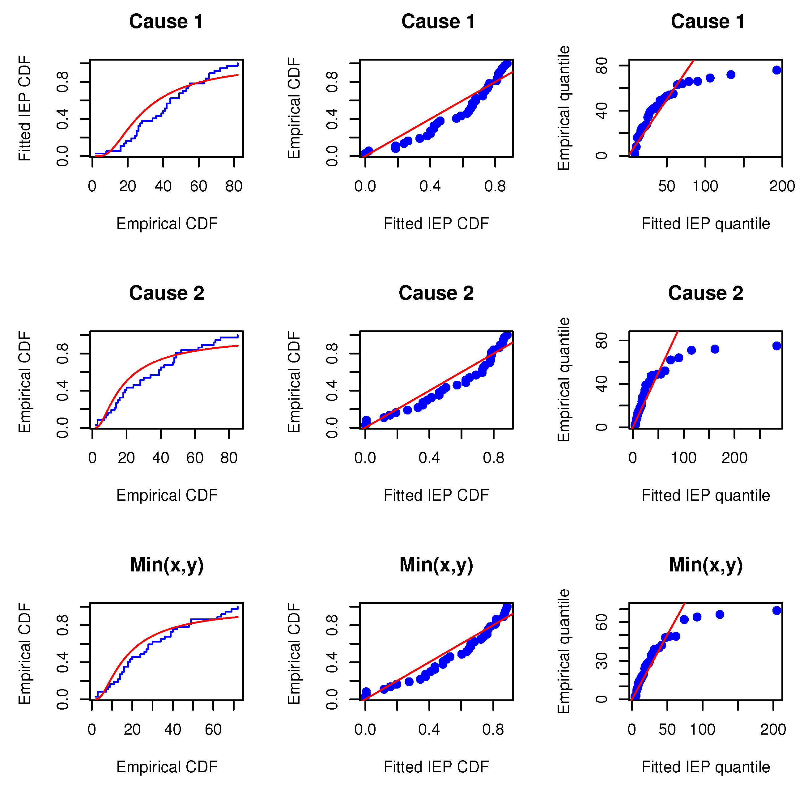
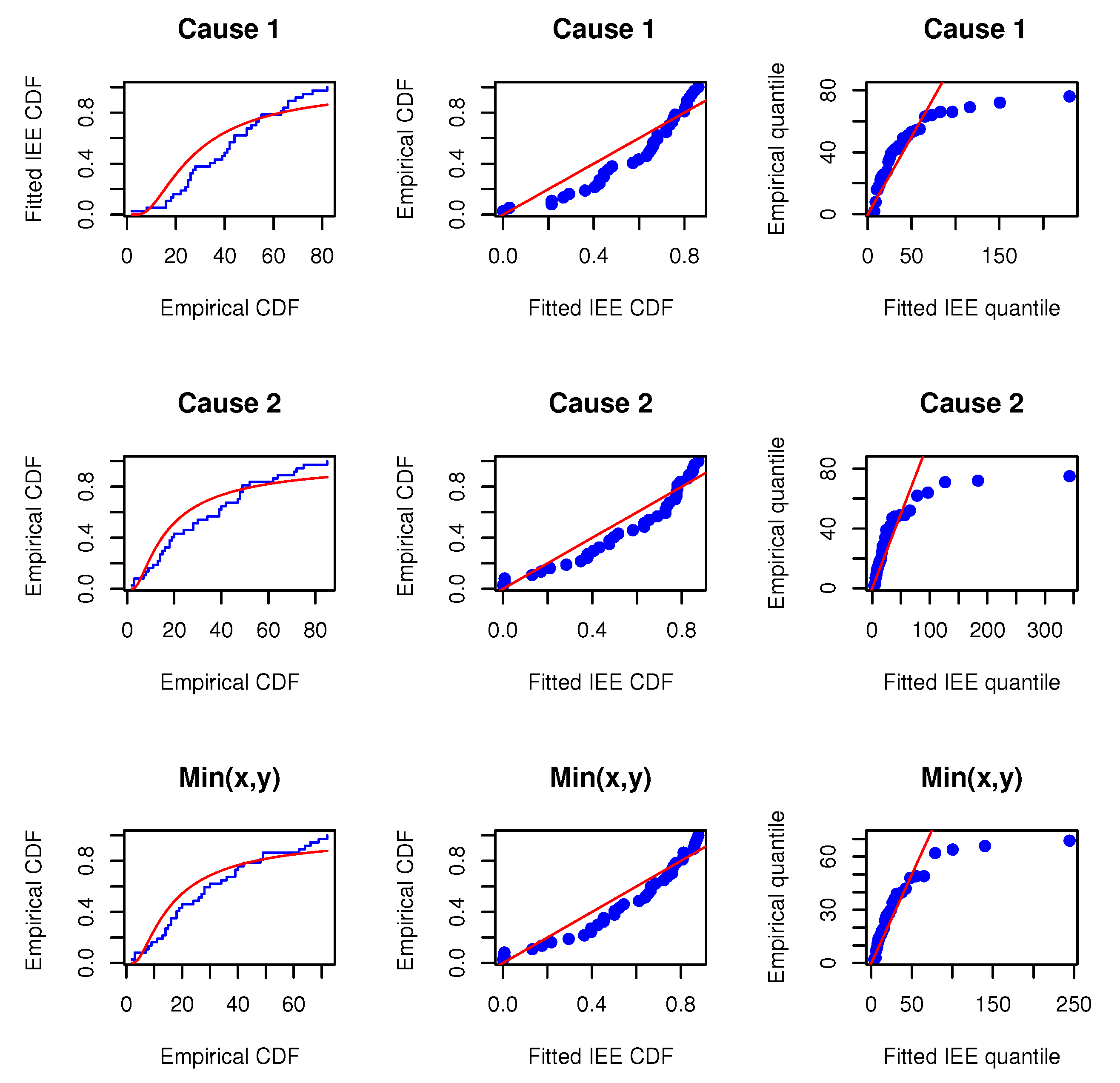
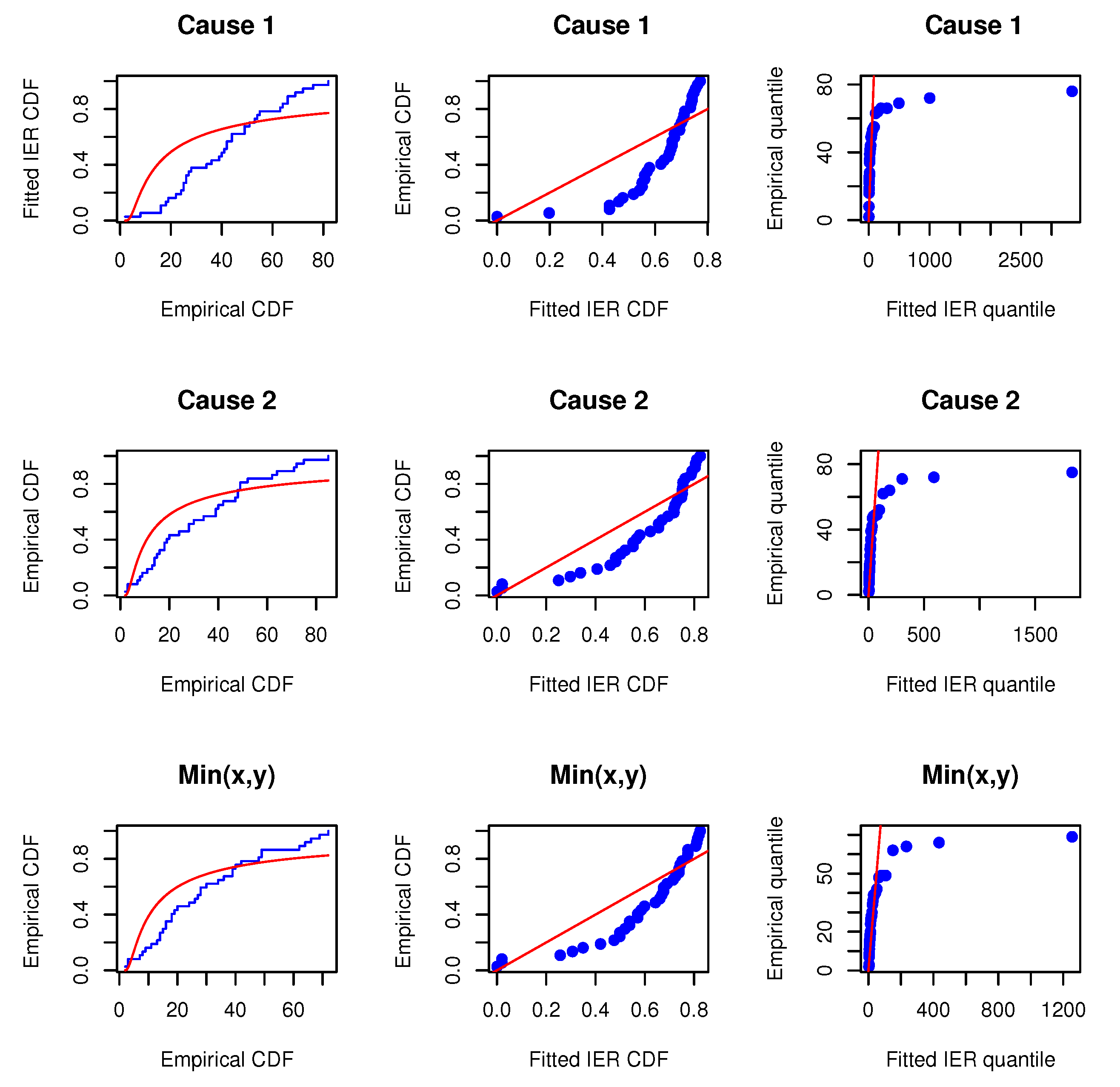
Before proceeding, we will verify whether the MOIEP distribution can be utilized to fit these real-life data. For this purpose, we compared their goodness-of-fit with two other distributions, i.e., the inverted exponentiated exponential (IEE) and the inverted exponentiated Rayleigh (IER) models. Additionally, two other models, i.e., the modified half-logistic (MHL) distribution (e.g., Shaheed [28]) and a new mixture of exponential and Weibull (MEW) distribution (e.g., Mohammad [29]) are considered for comparison. We evaluated the marginals and the minimum data to determine whether the IEP distribution provides a satisfactory fit compared to the other distributions. The Kolmogorov–Smirnov distances and p-values (within bracket) for data on X, Y, and $\min (X,Y)$ are calculated. The estimated results are reported in Table 6. Furthermore, the associated empirical cumulative distributions overlaying the theoretical cumulative distributions are plotted along with the probability–probability (PP) and the quantile–quantile (QQ) plots, as shown in Figure 2, Figure 3 and Figure 4. The estimated results and plots indicate that the IEP distribution fit is quite good compared to those of other models. Therefore, the proposed model can be used for fitting the marginals and minimums of the data for X and Y. Consequently, it may be concluded that the MOBIEP model is suitable for analyzing this football data.

Table 6. The Kolmogorov–Smirnov (K-S) statistic and the p-values of IER, IEE, and IEP for data on X, Y, and $min(X,Y)$.

Model	MLEs	K-S Statistic	p-Value
Data: X [Cause-I]
IER	$\widehat{\lambda }=40.0426,\widehat{\alpha }=0.2880$	0.3728	<0.0001
IEE	$\widehat{\lambda }=33.2001,\widehat{\alpha }=1.7976$	0.2156	0.0641
IEP	$\widehat{\lambda }=39.3260,\widehat{\alpha }=2.1339$	0.1938	0.1240
MHL	$\widehat{\lambda }=03.1599,\widehat{\alpha }=0.8754$	0.2379	0.0303
MEW	$\widehat{\lambda }=09.5126,\widehat{\alpha }=0.0358$	0.5854	<0.0001
Data: Y [Cause-II]
IER	$\widehat{\lambda }=24.1259,\widehat{\alpha }=0.3049$	0.2702	0.0090
IEE	$\widehat{\lambda }=15.1544,\widehat{\alpha }=1.1492$	0.1736	0.2148
IEP	$\widehat{\lambda }=17.9157,\widehat{\alpha }=1.2929$	0.1672	0.2523
MHL	$\widehat{\lambda }=03.8333,\widehat{\alpha }=0.6267$	0.1703	0.2333
MEW	$\widehat{\lambda }=09.3197,\widehat{\alpha }=0.0427$	0.5213	<0.0001
Data: $min(X,Y)$
IER	$\widehat{\lambda }=25.3403,\widehat{\alpha }=0.3272$	0.2862	0.0047
IEE	$\widehat{\lambda }=15.8981,\widehat{\alpha }=1.3048$	0.1806	0.1788
IEP	$\widehat{\lambda }=18.7962,\widehat{\alpha }=1.4818$	0.1608	0.2941
MHL	$\widehat{\lambda }=04.6139,\widehat{\alpha }=0.5926$	0.1945	0.1215
MEW	$\widehat{\lambda }=09.1112,\widehat{\alpha }=0.0485$	0.5242	<0.0001

Figure 2. Empirical distribution and fitted IEP models; PP and QQ plots for UEFA football data.

Figure 3. Empirical distribution and fitted IEE models; PP and QQ plots for UEFA football data.

Figure 4. Empirical distribution and fitted IER models; PP and QQ plots for UEFA football data.

From Table 5, three sets of artificial GPHC competing risk samples are obtained and presented in Table 7. The datasets are generated under the sample size $(n,m,k)=(37,30,26)$, with the censoring scheme $r_1=\cdots =r_{m-1}=0$ and $r_m=7$ with various monitoring points, T, and masking numbers, p. Various estimates for ${\alpha }_1,{\alpha }_2,{\alpha }_3$, and $\lambda$ are listed in Table 8, where the intervals are obtained with a significance level of $95\%$. In Table 8, the first two rows present point estimates along with their corresponding standard errors. The subsequent two groups of rows provide interval estimates. The associated interval lengths are obtained for asymptotic and Bayesian intervals. Bayes estimates are obtained using improper priors, and all the hyper-parameters are zeros. We observe from Table 8 under datasets I, II, and III that the MLEs and Bayes estimates are quite similar for the different model parameters. Furthermore, the behavior of the credible intervals is observed to be marginally better than that of the MLE-based intervals.

Table 7. GPHC competing risks for UEFA football data.

Data $\mathbf{I}:$ $\mathbf{T}=40$, $\mathbf{q}=1$, with $\mathbf{d}=26$
(2,0)	(3,2)	(7,2)	(8,0)	(9,2)	(11,2)
(13,2)	(14,2)	(15,2)	(16,1)	(16,0)	(18,3)
(18,2)	(19,0)	(20,2)	(24,0)	(26,1)	(27,1)
(28,0)	(30,2)	(34,0)	(36,1)	(39,0)	(39,2)
(40,0)	(42,0)	(48,2)	(49,0)	(62,2)	(64,2)
Data $\mathbf{II}:$ $\mathbf{T}=\mathbf{60}$, $\mathbf{q}=\mathbf{3}$, with $\mathbf{d}=\mathbf{28}$
(2,0)	(3,2)	(7,2)	(8,0)	(9,2)	(11,2)
(13,2)	(14,2)	(15,2)	(16,1)	(16,0)	(18,3)
(18,2)	(19,0)	(20,2)	(24,0)	(26,1)	(27,1)
(28,0)	(30,2)	(34,0)	(36,1)	(39,3)	(39,2)
(40,0)	(42,3)	(48,2)	(49,0)	(62,2)	(64,2)
Data $\mathbf{III}:$ $\mathbf{T}=\mathbf{70}$, $\mathbf{q}=\mathbf{2}$, with $\mathbf{d}=\mathbf{30}$
(2,0)	(3,2)	(7,2)	(8,0)	(9,2)	(11,2)
(13,2)	(14,2)	(15,2)	(16,1)	(16,0)	(18,3)
(18,2)	(19,0)	(20,2)	(24,0)	(26,1)	(27,1)
(28,0)	(30,2)	(34,0)	(36,1)	(39,3)	(39,2)
(40,0)	(42,0)	(48,2)	(49,0)	(62,2)	(64,2)

Table 8. Point and interval estimates of MOIEP parameters for the UEFA GPHC competing risks data.

Data I	${\mathit{\alpha }}_1$	${\mathit{\alpha }}_2$	${\mathit{\alpha }}_3$	$\mathit{\lambda }$
MLE	(0.1974, 0.1097)	(0.5428, 0.2103)	(0.4935, 0.1968)	(17.6101, 4.4784)
Bayes	(0.1801, 0.0783)	(0.5112, 0.1376)	(0.4697, 0.1399)	(17.4432, 1.9257)
ACI	(0.0177, 0.4125)	(0.1307, 0.9550)	(0.1076, 0.8794)	(8.8324, 26.3878)
	0.3948	0.8243	0.7718	17.5554
HPD	(0.0330, 0.3626)	(0.2092, 0.8117)	(0.2246, 0.7515)	(13.6773, 22.1700)
	0.3296	0.6025	0.5269	8.4927
Data II	${\mathit{\alpha }}_{\mathbf{1}}$	${\mathit{\alpha }}_{\mathbf{2}}$	${\mathit{\alpha }}_{\mathbf{3}}$	$\mathit{\lambda }$
MLE	(0.2149, 0.1196)	(0.6447, 0.2441)	(0.4835, 0.2000)	(17.5864, 4.4817)
Bayes	(0.1779, 0.0762)	(0.5674, 0.1316)	(0.4581, 0.1157)	(17.8511, 1.9884)
ACI	(0.0196, 0.4495)	(0.1662, 1.1232)	( 0.0914, 0.8756)	(8.8022, 26.3706)
	0.4299	0.9570	0.7842	17.5684
HPD	(0.0508, 0.3330)	(0.2829, 0.8352)	(0.1956, 0.8335)	(13.0136, 22.0701)
	0.2822	0.5523	0.6379	9.0565
Data III	${\mathit{\alpha }}_{\mathbf{1}}$	${\mathit{\alpha }}_{\mathbf{2}}$	${\mathit{\alpha }}_{\mathbf{3}}$	$\mathit{\lambda }$
MLE	(0.2051, 0.1124)	(0.7179, 0.2507)	(0.5128, 0.1989)	(18.8644, 4.4932)
Bayes	(0.1935, 0.0784)	(0.6936, 0.1591)	(0.4976, 0.1392)	(19.5147, 2.0666)
ACI	(0.0153, 0.4255)	(0.2264, 1.2094)	(0.1228, 0.9028)	(10.0577, 27.6712)
	0.4102	0.9830	0.7800	17.6135
HPD	(0.0507, 0.3912)	(0.3943, 1.1394)	(0.2298, 0.7220)	(15.1168, 24.3044)
	0.3405	0.7451	0.4922	9.1876

6. Conclusions

In this paper, inferences for the dependent competing risk model are discussed under the GPHC scheme. The Marshal–Olkin bivariate IEP distribution approach is employed to model dependent competing risk failure data. Various inferences for the unknown parameters are derived using classical and Bayesian methods in the presence of partially observed failure causes. The existence and uniqueness of the MLEs for the model parameters are established. Bayes point and interval estimates are computed on based flexible priors. The proposed sampling technique is used for this purpose. Generally, numerical findings have demonstrated that Bayes estimates yield superior results compared to likelihood estimates when the proper prior distribution is applied. Specifically, the intervals obtained from the Bayes methods are shorter in length than those based on the MLE intervals. Although a dependent MOBIEP-generalized, progressively hybrid, censoring-based competing risk model is discussed in this paper, further inferences incorporating the EM algorithm and bootstrap method also appear interesting, these will be discussed in future research.