Author Contributions
Conceptualization, M.M., B.A., I.M. and R.G.; methodology, M.M., J.X., B.A., I.M. and R.G.; software, M.M., B.A. and I.M.; validation, M.M., J.X., B.A., I.M. and R.G.; formal analysis, M.M., J.X., B.A., I.M. and R.G.; investigation, M.M., J.X., B.A., I.M. and R.G.; resources, M.M., J.X., B.A., I.M. and R.G.; data curation, M.M., J.X., B.A., I.M. and R.G.; writing—original draft preparation, M.M., B.A. and I.M.; writing—review and editing, M.M., J.X., B.A., I.M. and R.G.; visualization, M.M., J.X., B.A., I.M. and R.G.; supervision, M.M., J.X., B.A., I.M. and R.G.; project administration, M.M., J.X., B.A., I.M. and R.G.; funding acquisition, M.M., J.X. and R.G. All authors have read and agreed to the published version of the manuscript.
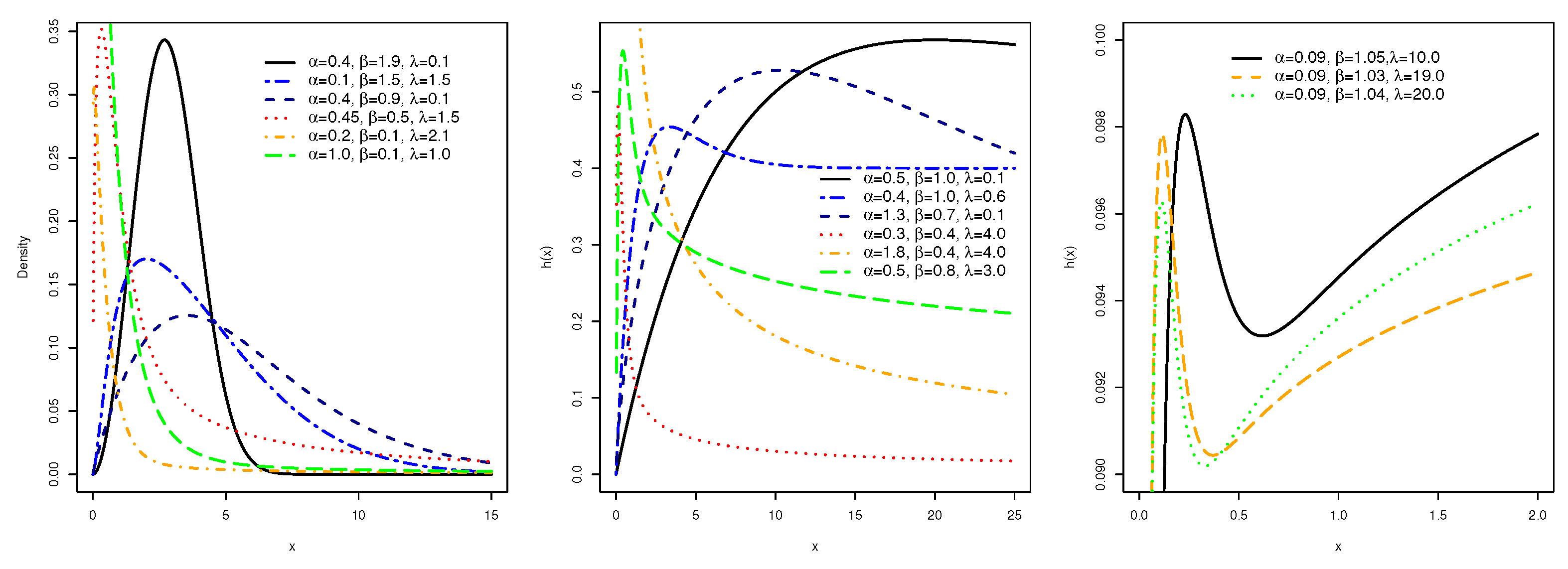
Figure 1.
Graphical illustrations of PDF and FRF of HWE model for some selected parameters.
Figure 1.
Graphical illustrations of PDF and FRF of HWE model for some selected parameters.
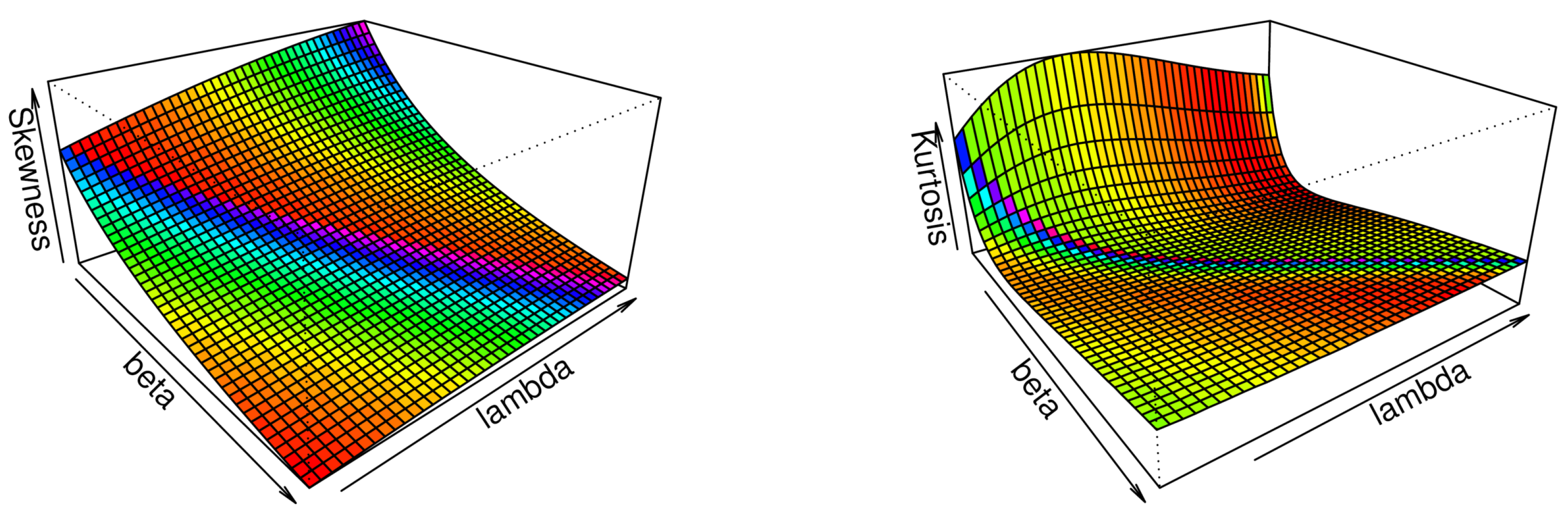
Figure 2.
Plots of the Bo and Mo for the HWE model for fixed .
Figure 2.
Plots of the Bo and Mo for the HWE model for fixed .
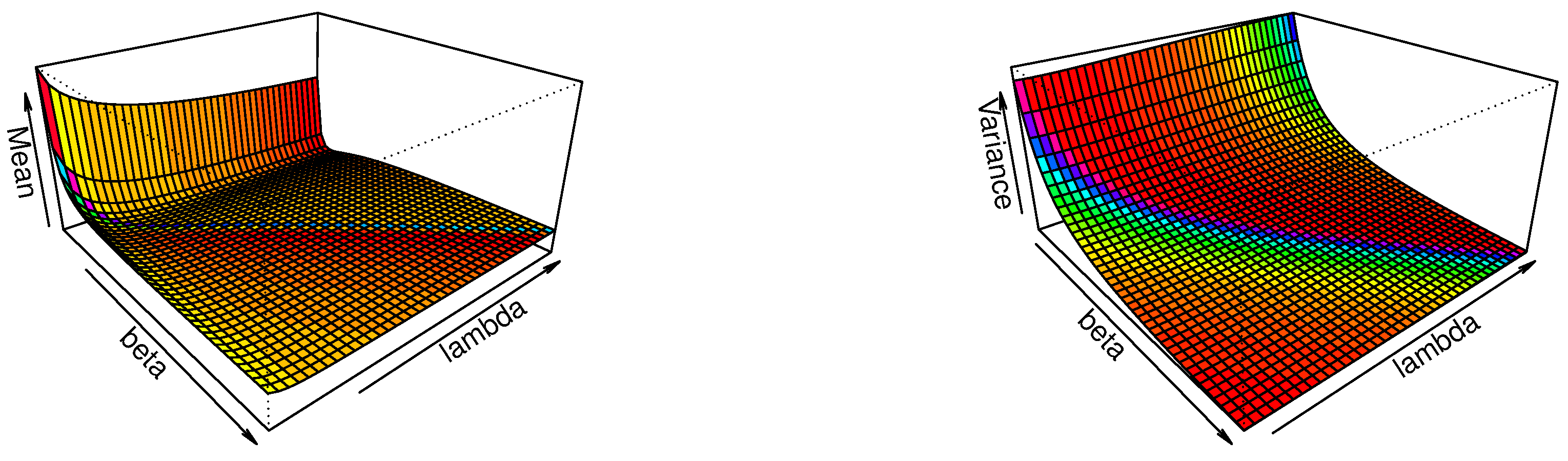
Figure 3.
Plots of mean (left) and variance (right) for the HWE model for fixed .
Figure 3.
Plots of mean (left) and variance (right) for the HWE model for fixed .
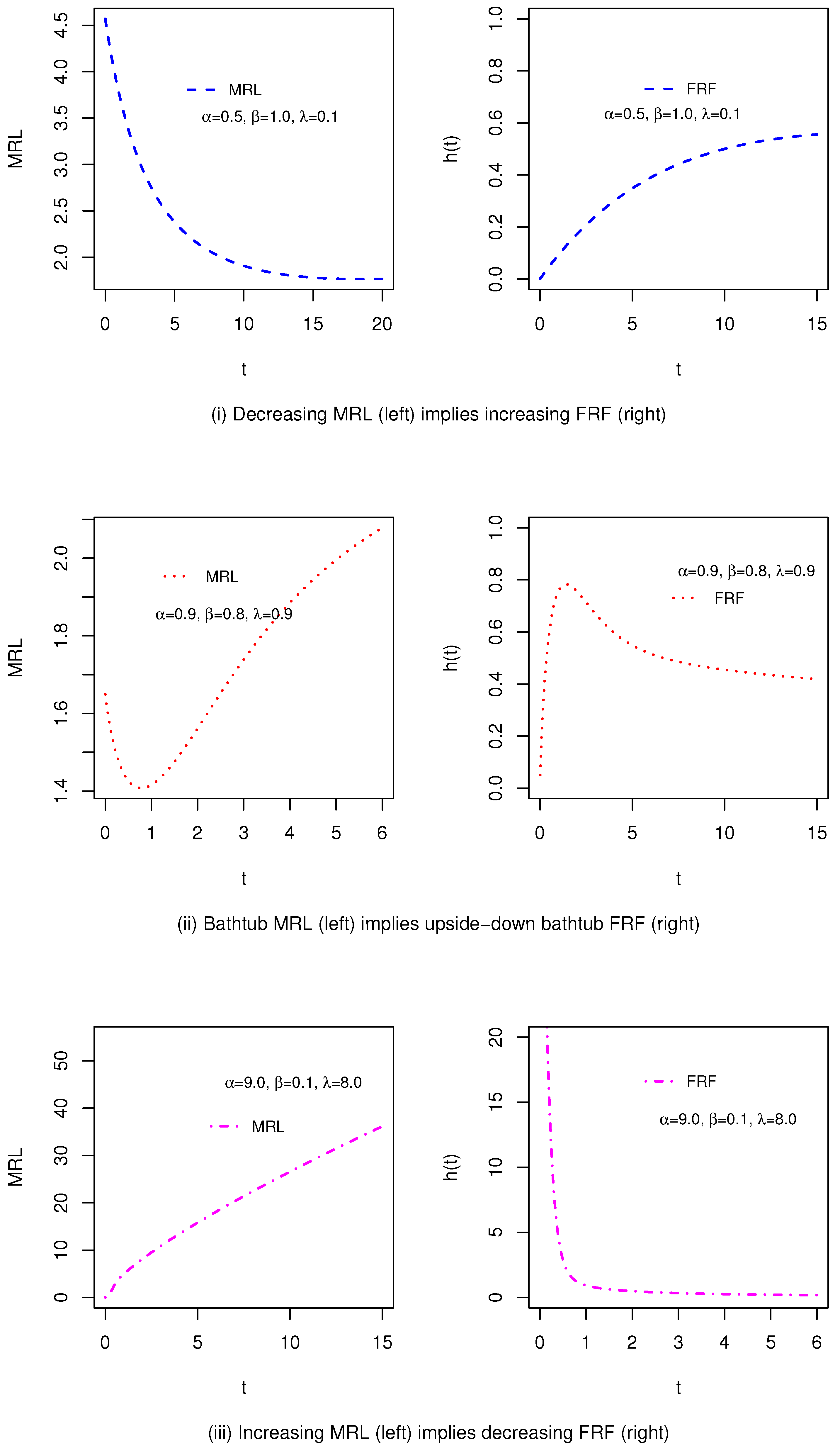
Figure 4.
Graphical presentation demonstrating the reciprocal relationship between the MRL and FRF of the proposed model for some selected parameters shown in (i–iii).
Figure 4.
Graphical presentation demonstrating the reciprocal relationship between the MRL and FRF of the proposed model for some selected parameters shown in (i–iii).
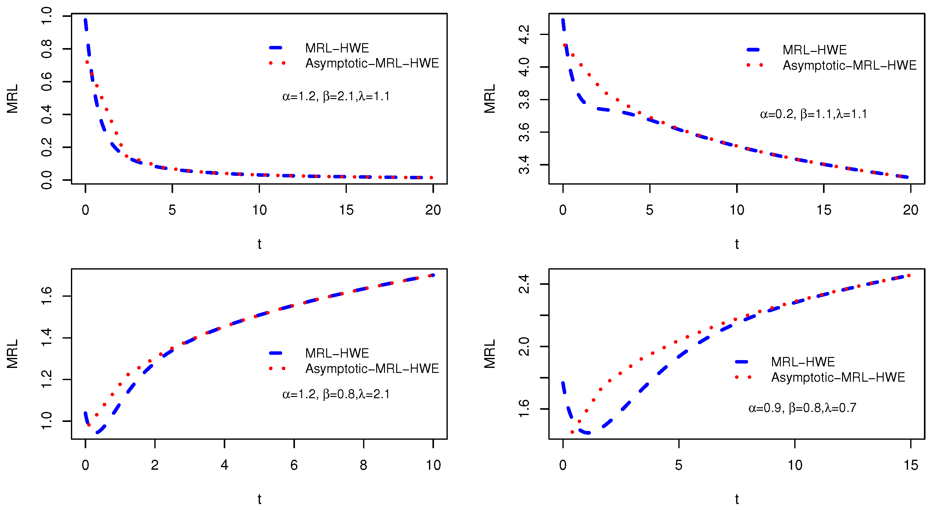
Figure 5.
Plots of the MRL and asymptote of the MRL of the HWE model.
Figure 5.
Plots of the MRL and asymptote of the MRL of the HWE model.
Figure 6.
Plots of the Ex and CRE of the HWE for a fixed value of .
Figure 6.
Plots of the Ex and CRE of the HWE for a fixed value of .
Figure 7.
Flowchart demonstrating the bootstrap samples for the .
Figure 7.
Flowchart demonstrating the bootstrap samples for the .
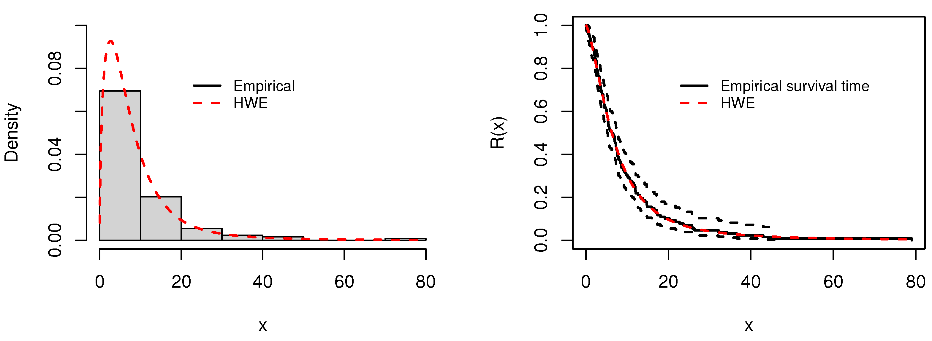
Figure 8.
Plots of the histogram and fitted PDF (left), and empirical and fitted survival functions (right), for the first data.
Figure 8.
Plots of the histogram and fitted PDF (left), and empirical and fitted survival functions (right), for the first data.
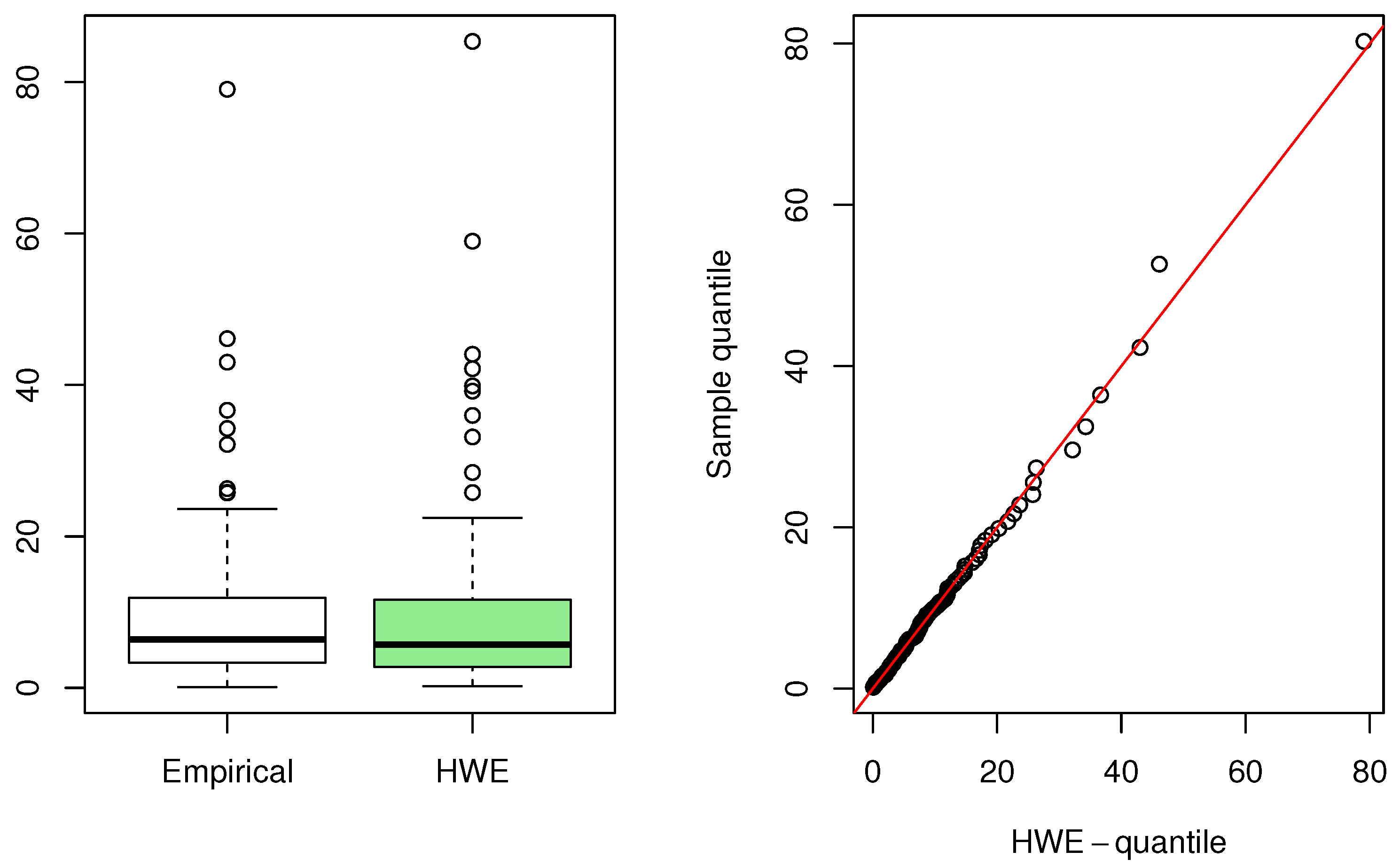
Figure 9.
Box plot (left) and quantile–quantile plot (right) for the first data.
Figure 9.
Box plot (left) and quantile–quantile plot (right) for the first data.
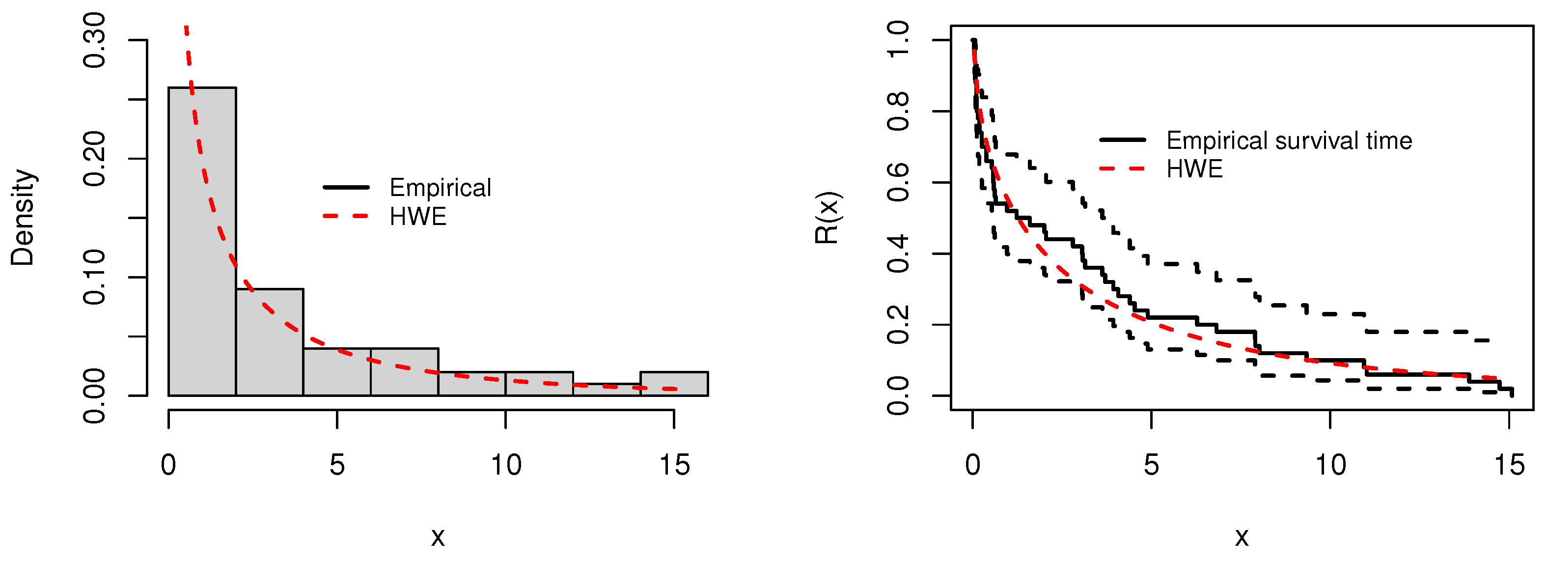
Figure 10.
Plots of the histogram and fitted PDF (left), and empirical and fitted survival functions (right), for the second data.
Figure 10.
Plots of the histogram and fitted PDF (left), and empirical and fitted survival functions (right), for the second data.
Figure 11.
Box plot (left) and quantile–quantile plot (right) for the second data.
Figure 11.
Box plot (left) and quantile–quantile plot (right) for the second data.
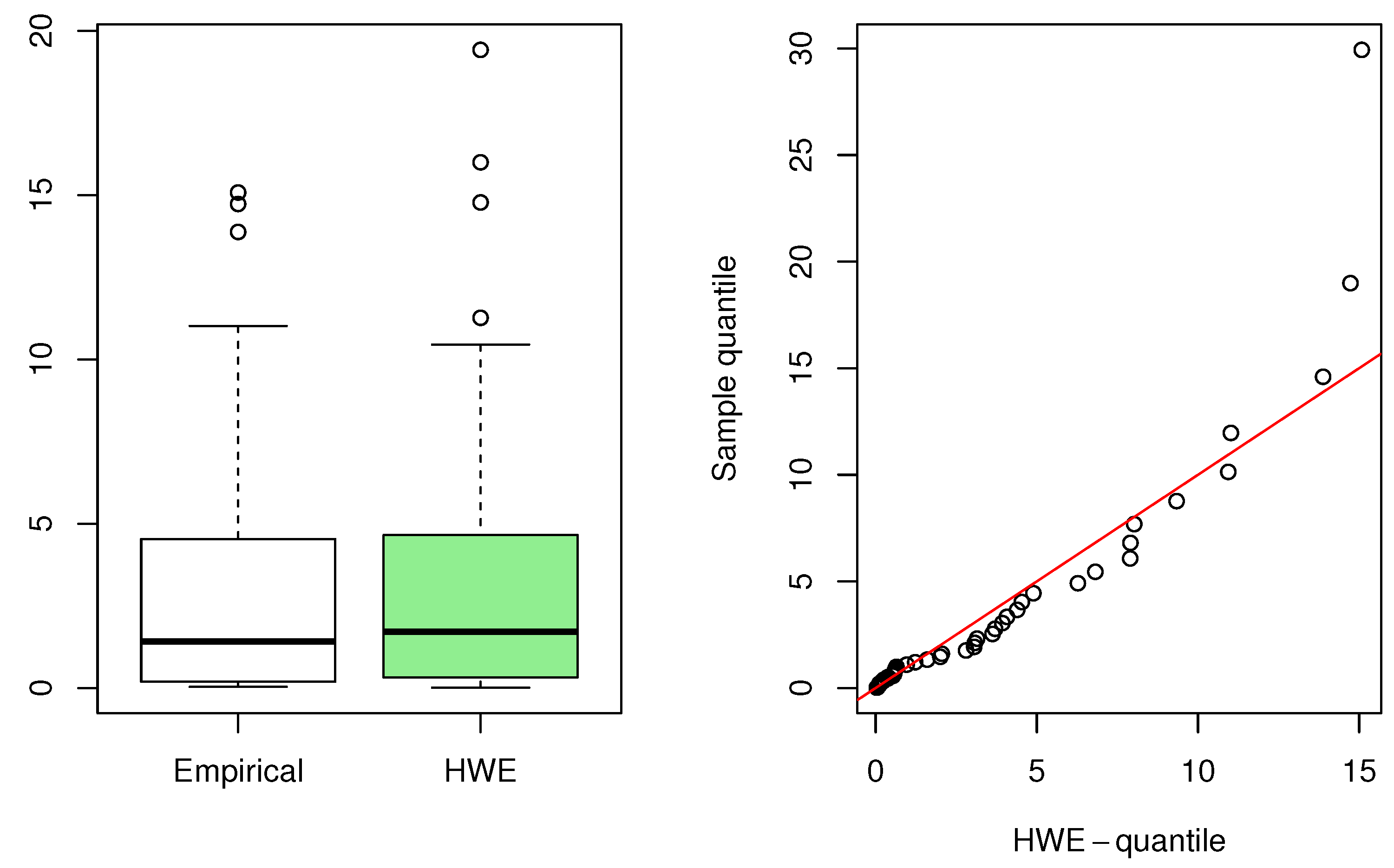
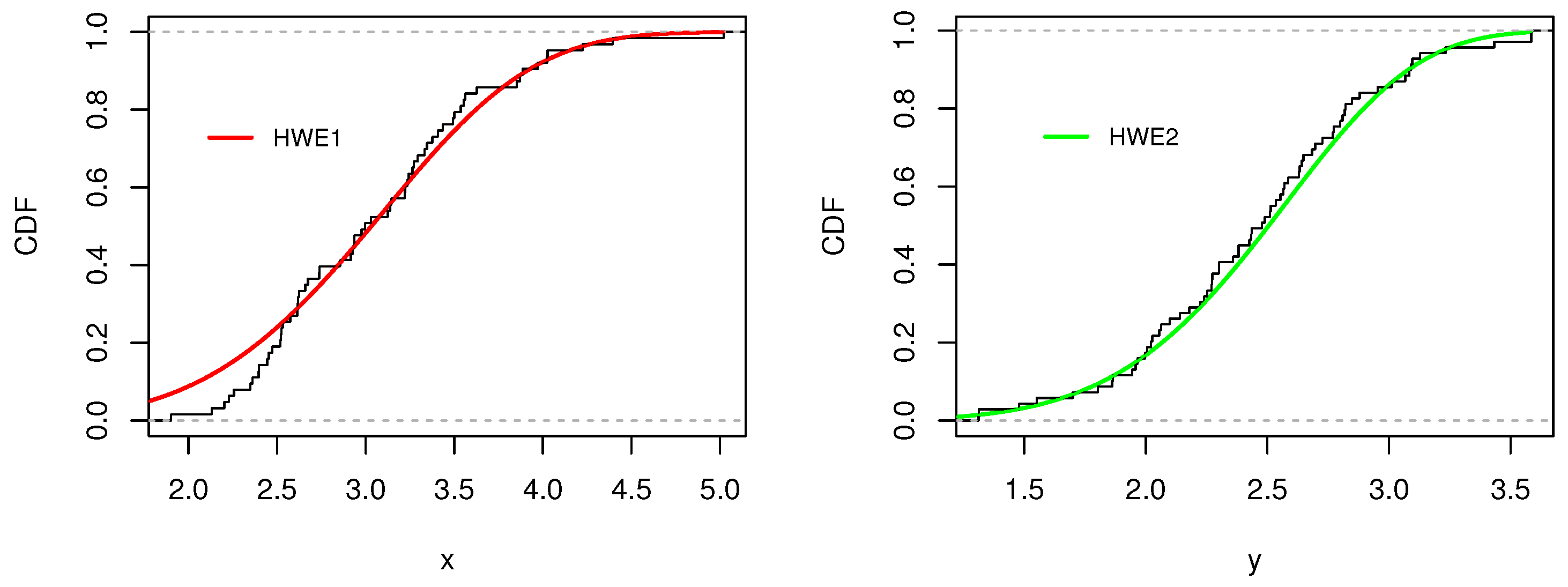
Figure 12.
Plots of the empirical and fitted and models for the SS-datasets.
Figure 12.
Plots of the empirical and fitted and models for the SS-datasets.
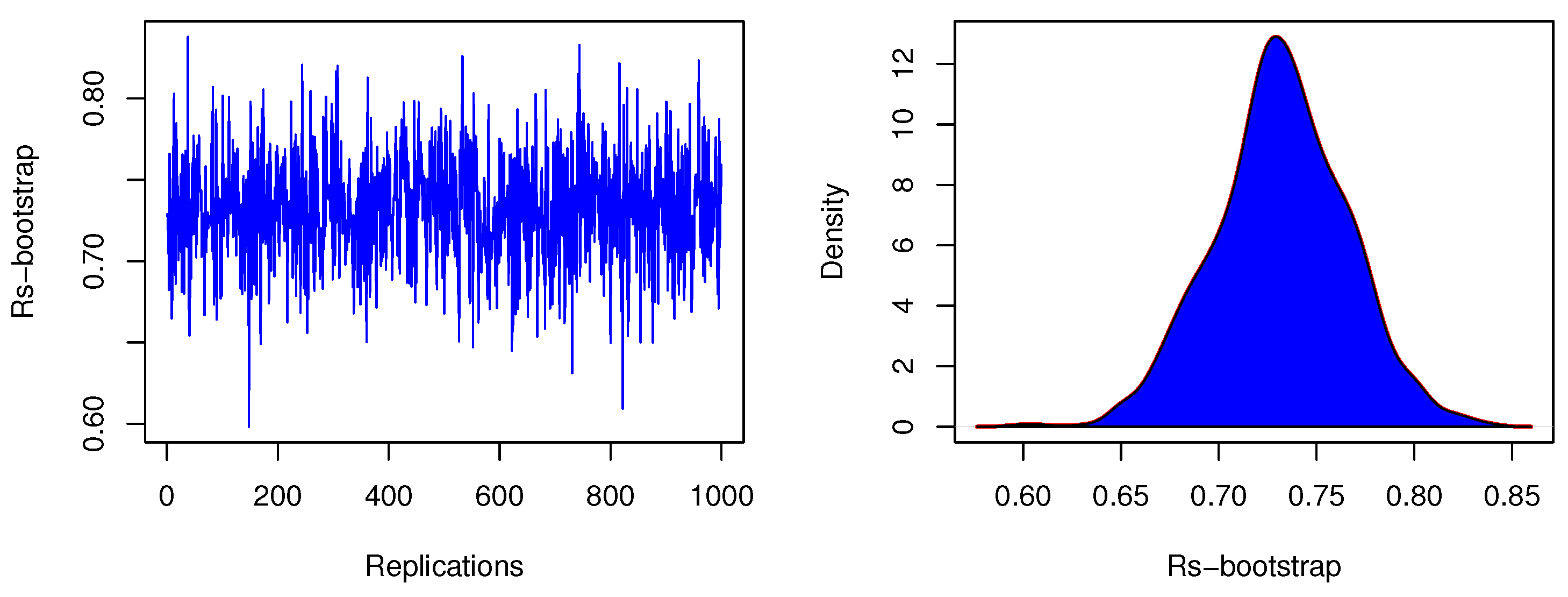
Figure 13.
Plots illustrating the estimated bootstrap values of and their density for the SS-datasets.
Figure 13.
Plots illustrating the estimated bootstrap values of and their density for the SS-datasets.
Figure 14.
Plots of the profile log-likelihood of the parameters for the SS-data.
Figure 14.
Plots of the profile log-likelihood of the parameters for the SS-data.
Table 1.
G-classes of distributions.
Table 1.
G-classes of distributions.
| Model Name | Cumulative Distribution Function |
|---|
| Beta-G [1] | |
| | where, is the incomplete beta function |
| Generalized beta-G [2] | |
| New Kumaraswamy-G [3] | |
| Kumaraswamy–Poisson-G [4] | |
| Poisson-odd generalized exponential-G [5] | |
| Extended Topp–Leone-G [6] | |
| Power Topp–Leone-G [7] | |
| Weighted cosine-G [8] | |
| Tan-G-loss family [9] | |
| Exponent-G-exponential [10] | |
Table 2.
Some possible functions and ranges.
Table 2.
Some possible functions and ranges.
| Name | | Range |
|---|
| Exponential | | |
| Exponent | | |
| Weibull | | |
| Extended Power | | |
| Hybrid-odd | | |
| Sine | | |
| Cosine | | |
| Tangent | | |
Table 3.
Numerical evaluation of identifiability of the HWE model based on some parameters values (
13).
Table 3.
Numerical evaluation of identifiability of the HWE model based on some parameters values (
13).
| Case I | Hypothesis and | (γ, δ) | Absolute Error |
|---|
| 1 | , | | |
| 2 | , | | |
| 3 | , | | |
| 4 | , | | |
| 5 | , | | |
| 6 | , | | |
| 7 | , | | |
| 8 | , | 0 | 0 |
| Case II | | | |
| 1 | , | | |
| 2 | , | | |
| 3 | , | | |
| 4 | , | | |
| 5 | , | | |
| 6 | , | | |
| 7 | , | | |
| 8 | , | 0 | 0 |
| Case III | | | |
| 1 | , | | |
| 2 | , | | |
| 3 | , | | |
| 4 | , | | |
| 5 | , | | |
| 6 | , | | |
| 7 | , | | |
| 8 | , | 0 | 0 |
Table 4.
Simulation results for HWE: the average estimate (AE), MSE, and Bias in parenthesis-I.
Table 4.
Simulation results for HWE: the average estimate (AE), MSE, and Bias in parenthesis-I.
| n | | | | | | | |
| 50 | AE | 1.1647 | 0.5215 | 1.0525 | 1.9986 | 0.6703 | 1.5355 |
| | MSE | 0.7286 | 0.0421 | 0.6053 | 0.1876 | 0.0895 | 0.7451 |
| | Bias | (1.0647) | (0.0215) | (0.9525) | (3.5986) | (0.0703) | (0.7355) |
| 100 | | 1.2153 | 0.5234 | 1.4455 | 1.5015 | 0.6379 | 1.9396 |
| | | 0.6799 | 0.0217 | 0.5096 | 0.1236 | 0.0569 | 0.2240 |
| | | (0.1153) | (0.0234) | (0.3455) | (1.1015) | (0.0379) | (0.3996) |
| 150 | | 1.1779 | 0.5088 | 1.2756 | 1.8160 | 0.6488 | 1.6290 |
| | | 0.2454 | 0.0137 | 0.5017 | 0.1173 | 0.0452 | 0.1857 |
| | | (0.0779) | (0.0088) | (0.1756) | (0.4160) | (0.0488) | (0.3690) |
| 200 | | 1.1249 | 0.5155 | 1.2585 | 1.4845 | 0.6326 | 1.6060 |
| | | 0.0865 | 0.0097 | 0.3963 | 0.0861 | 0.0357 | 0.0780 |
| | | (0.0249) | (0.0155) | (0.1585) | (0.2845) | (0.0326) | (0.2660) |
| n | | | | | | | |
| 50 | | 0.4686 | 0.6129 | 1.1136 | 0.5993 | 0.5249 | 0.7617 |
| | | 0.2696 | 0.0208 | 0.7570 | 0.7640 | 0.0217 | 1.4837 |
| | | (0.0686) | (0.0129) | (2.4136) | (0.0993) | (0.0249) | (0.2617) |
| 100 | | 0.4207 | 0.6112 | 1.0092 | 0.5410 | 0.5175 | 0.7202 |
| | | 0.0324 | 0.0106 | 0.3579 | 0.6182 | 0.0102 | 1.3801 |
| | | (0.0207) | (0.0112) | (0.3092) | (0.0410) | (0.0175) | (0.2202) |
| 150 | | 0.4117 | 0.6082 | 0.9483 | 0.5087 | 0.5086 | 0.5573 |
| | | 0.0310 | 0.0064 | 0.2896 | 0.0194 | 0.0055 | 0.0523 |
| | | (0.0117) | (0.0082) | (0.2483) | (0.0087) | (0.0086) | (0.0573) |
| 200 | | 0.4091 | 0.6059 | 0.7651 | 0.5045 | 0.5086 | 0.5580 |
| | | 0.0093 | 0.0048 | 0.0877 | 0.0134 | 0.0046 | 0.0142 |
| | | (0.0091) | (0.0059) | (0.0651) | (0.0045) | (0.0086) | (0.0580) |
| n | | | | | | | |
| 50 | | 0.6297 | 0.5232 | 0.9092 | 0.3227 | 0.5219 | 0.4598 |
| | | 0.2717 | 0.0170 | 1.8623 | 0.0422 | 0.0128 | 0.7901 |
| | | (0.1297) | (0.0232) | (0.3092) | (0.0227) | (0.0219) | (0.1598) |
| 100 | | 0.5216 | 0.5139 | 0.7284 | 0.3114 | 0.5077 | 0.4754 |
| | | 0.0917 | 0.0087 | 0.3203 | 0.0131 | 0.0057 | 0.6813 |
| | | (0.0216) | (0.0139) | (0.1284) | (0.0114) | (0.0077) | (0.1754) |
| 150 | | 0.5123 | 0.5078 | 0.6834 | 0.3032 | 0.5084 | 0.3400 |
| | | 0.0222 | 0.0053 | 0.2814 | 0.0062 | 0.0040 | 0.0688 |
| | | (0.0123) | (0.0078) | (0.0834) | (0.0032) | (0.0084) | (0.0400) |
| 200 | | 0.5090 | 0.5040 | 0.6375 | 0.3036 | 0.5057 | 0.3211 |
| | | 0.0111 | 0.0035 | 0.0435 | 0.0047 | 0.0029 | 0.0140 |
| | | (0.0090) | (0.0040) | (0.0375) | (0.0036) | (0.0057) | (0.0211) |
| n | | | | | | | |
| 50 | | 0.7147 | 0.7650 | 1.0193 | 0.5665 | 0.6335 | 0.5399 |
| | | 0.8917 | 0.0858 | 1.0267 | 1.7151 | 0.0321 | 0.4472 |
| | | (2.9147) | (−0.0350) | (0.2193) | (0.1665) | (0.0335) | (0.5399) |
| 100 | | 0.8418 | 0.7839 | 0.9830 | 0.4531 | 0.6103 | 0.5258 |
| | | 0.5853 | 0.0592 | 0.6344 | 0.0893 | 0.0168 | 0.3194 |
| | | (1.0418) | (−0.0161) | (0.1830) | (0.0531) | (0.0103) | (0.1258) |
| 150 | | 1.3960 | 0.7783 | 0.9133 | 0.4310 | 0.6107 | 0.4760 |
| | | 0.5329 | 0.0478 | 0.4175 | 0.0626 | 0.0115 | 0.0842 |
| | | (0.5960) | (−0.0217) | (0.1133) | (0.0310) | (0.0107) | (0.0760) |
| 200 | | 1.0949 | 0.7952 | 0.9480 | 0.4201 | 0.6079 | 0.4593 |
| | | 0.4051 | 0.0371 | 0.4013 | 0.0464 | 0.0087 | 0.0655 |
| | | (0.2949) | (−0.0048) | (0.1480) | (0.0201) | (0.0079) | (0.0593) |
Table 5.
Simulation results for HWE: the average estimate (AE), MSE, and Bias in parenthesis-II.
Table 5.
Simulation results for HWE: the average estimate (AE), MSE, and Bias in parenthesis-II.
| n | | | | | | | |
| 50 | AE | 0.1044 | 0.5232 | 0.2293 | 0.5777 | 0.6131 | 1.1722 |
| | MSE | 0.0068 | 0.0087 | 1.2860 | 0.7409 | 0.0218 | 1.5306 |
| | Bias | (0.0044) | (0.0232) | (0.3293) | (0.1777) | (0.0131) | (0.4722) |
| 100 | | 0.1023 | 0.5105 | 0.2808 | 0.4282 | 0.6058 | 0.9120 |
| | | 0.0016 | 0.0039 | 1.2025 | 0.0599 | 0.0103 | 1.0262 |
| | | (0.0023) | (0.0105) | (0.1808) | (0.0282) | (0.0058) | (0.2120) |
| 150 | | 0.1006 | 0.5077 | 0.1517 | 0.4102 | 0.6081 | 0.8076 |
| | | 0.0009 | 0.0026 | 0.0587 | 0.0174 | 0.0067 | 0.4280 |
| | | (0.0006) | (0.0077) | (0.0517) | (0.0102) | (0.0081) | (0.1076) |
| 200 | | 0.1019 | 0.5035 | 0.1203 | 0.4036 | 0.6091 | 0.7943 |
| | | 0.0007 | 0.0019 | 0.0146 | 0.0088 | 0.0048 | 0.1282 |
| | | (0.0019) | (0.0035) | (0.0203) | (0.0036) | (0.0091) | (0.0943) |
| n | | | | | | | |
| 50 | | 0.4072 | 0.3109 | 0.5049 | 2.3740 | 0.8766 | 1.1057 |
| | | 0.0153 | 0.0031 | 0.9124 | 1.3627 | 0.0972 | 1.1911 |
| | | (0.0072) | (0.0109) | (0.1049) | (3.4740) | (−0.0234) | (0.2057) |
| 100 | | 0.4076 | 0.3031 | 0.4218 | 1.6541 | 0.8622 | 1.0649 |
| | | 0.0077 | 0.0014 | 0.0190 | 0.7120 | 0.0777 | 0.8293 |
| | | (0.0076) | (0.0031) | (0.0218) | (1.7541) | (−0.0378) | (0.1649) |
| 150 | | 0.4017 | 0.3029 | 0.4200 | 1.7929 | 0.8673 | 1.0268 |
| | | 0.0043 | 0.0008 | 0.0114 | 0.0845 | 0.0596 | 0.6346 |
| | | (0.0017) | (0.0029) | (0.0200) | (0.8929) | (−0.0327) | (0.1268) |
| 200 | | 0.4027 | 0.3025 | 0.4137 | 1.3375 | 0.8809 | 1.0378 |
| | | 0.0036 | 0.0006 | 0.0096 | 0.0197 | 0.0471 | 0.5277 |
| | | (0.0027) | (0.0025) | (0.0137) | (0.4375) | (−0.0191) | (0.1378) |
| n | | | | | | | |
| 50 | | 1.4472 | 0.8512 | 0.3481 | 1.5807 | 1.0737 | 1.2864 |
| | | 0.6709 | 0.0949 | 0.1440 | 0.8743 | 0.1247 | 0.5345 |
| | | (1.1472) | (−0.0488) | (0.0481) | (4.4807) | (−0.0263) | (0.1864) |
| 100 | | 1.0783 | 0.8539 | 0.3353 | 1.4598 | 1.0450 | 1.2122 |
| | | 0.4591 | 0.0722 | 0.0738 | 0.8636 | 0.0907 | 0.1647 |
| | | (0.7783) | (−0.0461) | (0.0353) | (2.3598) | (−0.0550) | (0.1122) |
| 150 | | 0.7613 | 0.8472 | 0.3092 | 1.5477 | 1.0681 | 1.2462 |
| | | 0.5897 | 0.0540 | 0.0460 | 0.8000 | 0.0757 | 0.0507 |
| | | (0.4613) | (−0.0528) | (0.0092) | (1.4477) | (−0.0319) | (0.1462) |
| 200 | | 0.9864 | 0.8538 | 0.3067 | 1.7882 | 1.0840 | 1.2905 |
| | | 0.3148 | 0.0465 | 0.0386 | 0.5194 | 0.0574 | 0.0201 |
| | | (0.2864) | (−0.0462) | (0.0067) | (0.6882) | (−0.0160) | (0.1905) |
| n | | | | | | | |
| 50 | | 1.2415 | 1.1620 | 1.4288 | 0.5724 | 0.0504 | 0.6447 |
| | | 0.0672 | 0.1382 | 0.9878 | 0.2326 | 0.0927 | 0.3110 |
| | | (0.9415) | (−0.0380) | (0.1288) | (0.4724) | (−0.0496) | (0.5447) |
| 100 | | 1.2692 | 1.1377 | 1.4034 | 0.5909 | 0.0472 | 0.6221 |
| | | 0.0460 | 0.0992 | 0.5514 | 0.2018 | 0.0028 | 0.2776 |
| | | (0.9692) | (−0.0623) | (0.1034) | (0.4909) | (−0.0528) | (0.5221) |
| 150 | | 1.0112 | 1.1631 | 1.4532 | 0.5936 | 0.064 | 0.6122 |
| | | 0.0379 | 0.0786 | 0.3995 | 0.1036 | 0.0020 | 0.2048 |
| | | (0.7112) | (−0.0369) | (0.1532) | (0.4936) | (−0.0536) | (0.5122) |
| 200 | | 1.0366 | 1.1696 | 1.4625 | 0.5032 | 0.0463 | 0.6060 |
| | | 0.0148 | 0.0308 | 0.2053 | 0.0115 | 0.0002 | 0.1006 |
| | | (0.2366) | (−0.0304) | (0.1625) | (0.4932) | (−0.0537) | (0.5060) |
Table 6.
Parameter values, , with (SD) below, MSE of with (bias) below, and ALCI with (CP) below in parenthesis.
Table 6.
Parameter values, , with (SD) below, MSE of with (bias) below, and ALCI with (CP) below in parenthesis.
| () | | () | (SD) | (bias) | (CP) | (CP) |
|---|
| 0.4965 | (20,20) | 0.4966 | 0.00026 | 0.0807 | 0.0836 |
| | | | (0.0162) | (0.0012) | (0.98) | (0.99) |
| | | (20,30) | 0.4967 | 0.00021 | 0.0695 | 0.0719 |
| | | | (0.01436) | (0.00020) | (0.98) | (0.98) |
| | | (40,50) | 0.4966 | | 0.0422 | 0.0446 |
| | | | (0.0089) | (0.00011) | (0.98) | (0.96) |
| | | (60,60) | 0.4965 | | 0.0335 | 0.0355 |
| | | | (0.0075) | () | (0.97) | (0.98) |
| 0.6356 | (20,20) | 0.6374 | 0.0021 | 0.1821 | 0.1689 |
| | | | (0.0459) | (0.0019) | (0.93) | (0.92) |
| | | (20,30) | 0.6342 | 0.0017 | 0.1606 | 0.1465 |
| | | | (0.0407) | (−0.0036) | (0.94) | (0.91) |
| | | (40,50) | 0.6358 | 0.0008 | 0.1178 | 0.1098 |
| | | | (0.0295) | (0.0003) | (0.95) | (0.93) |
| | | (60,60) | 0.6348 | 0.00067 | 0.1011 | 0.0956 |
| | | | (0.0259) | (−0.00073) | (0.95) | (0.93) |
| 0.5046 | (20,20) | 0.5050 | 0.00045 | 0.1008 | 0.0981 |
| | | | (0.0213) | (0.0003) | (0.98) | (0.96) |
| | | (20,30) | 0.5059 | 0.00037 | 0.0875 | 0.0813 |
| | | | (0.0192) | (0.0013) | (0.97) | (0.98) |
| | | (40,50) | 0.5056 | 0.00018 | 0.0562 | 0.0526 |
| | | | (0.01333) | (0.0009) | (0.96) | (0.97) |
| | | (60,60) | 0.5047 | 0.00012 | 0.0456 | 0.0434 |
| | | | (0.0108) | () | (0.96) | (0.98) |
| 0.4815 | (20,20) | 0.4817 | 0.00076 | 0.1232 | 0.1323 |
| | | | (0.0276) | (0.00018) | (0.95) | (0.96) |
| | | (20,30) | 0.4832 | 0.00065 | 0.1075 | 0.1117 |
| | | | (0.0254) | (0.0017) | (0.94) | (0.95) |
| | | (40,50) | 0.4818 | 0.00036 | 0.0734 | 0.0772 |
| | | | (0.0189) | (0.00034) | (0.93) | (0.94) |
| | | (60,60) | 0.4801 | 0.00023 | 0.06121 | 0.0656 |
| | | | (0.0152) | (−0.00095) | (0.95) | (0.96) |
| 0.3074 | (20,20) | 0.3067 | 0.0059 | 0.3015 | 0.2887 |
| | | | (0.0772) | (−0.00066) | (0.94) | (0.93) |
| | | (20,30) | 0.3069 | 0.0049 | 0.2732 | 0.2598 |
| | | | (0.0702) | (−0.00051) | (0.94) | (0.93) |
| | | (40,50) | 0.3052 | 0.0028 | 0.2006 | 0.1943 |
| | | | (0.0531) | (−0.0021) | (0.94) | (0.92) |
| | | (60,60) | 0.3087 | 0.0019 | 0.1735 | 0.1698 |
| | | | (0.0444) | (0.0014) | (0.94) | (0.94) |
| 0.500 | (20,20) | 0.4995 | 0.0028 | 0.0798 | 0.0806 |
| | | | (0.0168) | (−0.0044) | (0.98) | (0.98) |
| | | (20,30) | 0.4998 | 0.0017 | 0.0668 | 0.0702 |
| | | | (0.0134) | (−0.00018) | (0.98) | (0.96) |
| | | (40,50) | 0.4997 | | 0.0418 | 0.0429 |
| | | | (0.0095) | (−0.00029) | (0.97) | (0.98) |
| | | (60,60) | 0.4997 | | 0.0324 | 0.0326 |
| | | | (0.0075) | (−0.00025) | (0.96) | (0.97) |
| 0.4999 | (20,20) | 0.4997 | 0.0022 | 0.1881 | 0.1906 |
| | | | (0.4704) | (−0.0003) | (0.89) | (0.90) |
| | | (20,30) | 0.4948 | 0.0017 | 0.1615 | 0.1740 |
| | | | (0.0409) | (−0.0052) | (0.91) | (0.93) |
| | | (40,50) | 0.5001 | 0.0008 | 0.1075 | 0.1109 |
| | | | (0.0285) | (0.0001) | (0.92) | (0.94) |
| | | (60,60) | 0.5001 | 0.0006 | 0.0906 | 0.0903 |
| | | | (0.0239) | (0.0006) | (0.92) | (0.93) |
| 0.6993 | (20,20) | 0.7016 | 0.0058 | 0.2904 | 0.3032 |
| | | | (0.0759) | (0.0023) | (0.93) | (0.94) |
| | | (20,30) | 0.7027 | 0.0049 | 0.2614 | 0.2683 |
| | | | (0.0704) | (0.0034) | (0.93) | (0.93) |
| | | (40,50) | 0.6979 | 0.0028 | 0.1961 | 0.2009 |
| | | | (0.0529) | (−0.0014) | (0.93) | (0.94) |
| | | (60,60) | 0.6999 | 0.0019 | 0.1683 | 0.1720 |
| | | | (0.0130) | (0.0007) | (0.94) | (0.95) |
Table 7.
Reliability function of the competing distributions .
Table 7.
Reliability function of the competing distributions .
| Distribution | R(x) |
|---|
| Modified Weibull (MW) [18] | |
| Exponentiated Weibull (EW) [45] | |
| Exponentiated sine Weibull (ESW) [46] | |
| Additive Weibull (AddW) [47] | |
| Sarhan–Zaindin modified Weibull (SZW) [48] | |
| Modified Weibull extension (MWE) [20] | |
| Extended cosine Weibull (ESW) [49] | |
Table 8.
MLEs for first datasets.
Table 8.
MLEs for first datasets.
| Distribution | | | | |
|---|
| HWE | 0.592 (0.6431) | 0.5103 (0.2616) | 0.0973 (0.08700) | - |
| W | 0.0939 (0.0190) | 1.0478 (0.0675) | - | - |
| MW | 0.0939 (0.0172) | 1.2 (1.0035) | 1.0478 (0.0955) | - |
| EW | 0.4539 (0.2386) | 0.6542 (0.1338) | 2.7973 (1.2577) | - |
| AddW | 0.0120 (5.2031) | 1.0480 (0.1545) | 0.0818(7.8070) | 1.0477 (0.0415) |
| MWE | 1.5 (0.5461) | 1.0490 (0.8420) | 1.6740 (0.1306) | - |
| ESW | 2.7589 (1.0894) | 0.6208 (0.1138) | 0.2666 (0.1174) | - |
| ECSW | 0.3199 (0.0282) | 0.1749 (0.0001) | 1.0030 (1.1 ) | - |
Table 9.
L, AIC, BIC, CAIC, A, W, KS, and p-value for first data sets.
Table 9.
L, AIC, BIC, CAIC, A, W, KS, and p-value for first data sets.
| Distribution | L | | | CAIC | A | W | (PV) |
|---|
| HWE | −409.80 | 825.61 | 834.17 | 825.80 | 0.1234 | 0.0174 | 0.0310 (0.9997) |
| W | −414.09 | 832.17 | 837.88 | 832.27 | 0.7817 | 0.1309 | 0.0701 (0.5552) |
| MW | −414.09 | 834.17 | 842.73 | 834.37 | 0.7815 | 0.1308 | 0.0704 (0.5507) |
| EW | −410.68 | 827.36 | 835.92 | 827.55 | 0.2885 | 0.0437 | 0.0450 (0.9578) |
| AddW | −414.09 | 836.17 | 847.58 | 836.49 | 0.1314 | 0.7863 | 0.0700 (0.5573) |
| MWE | −414.08 | 834.18 | 842.73 | 834.37 | 0.7831 | 0.1311 | 0.0710 (0.5388) |
| ESW | −410.48 | 826.95 | 835.51 | 827.15 | 0.2595 | 0.0394 | 0.0436 (0.9682) |
| ECSW | −413.44 | 832.88 | 841.44 | 833.07 | 0.6917 | 0.1154 | 0.0660 (0.6335) |
Table 10.
MLEs for second dataset.
Table 10.
MLEs for second dataset.
| Distribution | | | | |
|---|
| HWE | (0.6015) (0.1123) | 0.5989 (0.0785) | 13.5171 (6.2122) | - |
| W | 0.5412 (0.0995) | 0.6611 (0.0747) | - | - |
| MW | 0.4964 (0.0.0990) | 0.5615 (0.0975) | 0.0335 (0.0248) | - |
| EW | 0.3859 (1.1141) | 0.7698 (0.9441) | 0.7856 (1.4754) | - |
| AddW | 0.5289 (8.8612) | 0.6611 (0.0830) | 0.0124 (8.8614) | 0.6603 (1.5778) |
| SZMW | 0.4926 (0.1807) | 0.6197 (0.1544) | 0.0438 (0.1314) | - |
| MWE | 21.4159 (7.0007) | 0.5845 (0.0766) | 0.1319 (0.0264) | - |
| ESW | 0.4288 (0.7410) | 1.1379 (1.5183) | 0.0695 (0.3030) | - |
| ECSW | 6.3682 (7.0763) | 0.0528 (0.0582) | 0.6489 (0.0744) | - |
Table 11.
L, AIC, BIC, CAIC, A, W, KS, and p-value for second datasets.
Table 11.
L, AIC, BIC, CAIC, A, W, KS, and p-value for second datasets.
| Distribution | L | | | CAIC | W | A | (PV) |
|---|
| HWE | −99.07 | 204.15 | 209.88 | 204.67 | 0.6765 | 0.1109 | 0.1122 (0.5186) |
| W | −102.36 | 208.73 | 212.55 | 208.98 | 0.9393 | 0.1507 | 0.1269 (0.3652) |
| MW | −101.36 | 208.73 | 214.46 | 209.25 | 0.8504 | 0.1300 | 0.1326 (0.3144) |
| EW | −102.37 | 210.71 | 216.45 | 211.23 | 0.9459 | 0.1499 | 0.1333 (0.3083) |
| AddW | −102.36 | 212.73 | 220.38 | 213.62 | 0.9393 | 0.1507 | 0.1270 (0.3642) |
| SZMW | −102.32 | 210.64 | 216.38 | 211.16 | 0.9304 | 0.1487 | 0.1278 (0.3563) |
| MWE | −101.94 | 209.88 | 215.62 | 210.40 | 0.8908 | 0.1402 | 0.1375 (0.2747) |
| ESW | −102.51 | 211.02 | 216.76 | 211.54 | 0.9417 | 0.1453 | 0.1504 (0.1877) |
| ECSW | −102.30 | 210.59 | 216.33 | 211.11 | 0.1489 | 0.9305 | 0.1289 (0.3471) |
Table 12.
MLEs, , , KS with p-value in parenthesis, and ALCI with CI within parentheses for the stress–strength dataset.
Table 12.
MLEs, , , KS with p-value in parenthesis, and ALCI with CI within parentheses for the stress–strength dataset.
| | | | | | |
|---|
| 111.4004 | 0.1057 | 0.0654 | 0.7299 | 0.1323 | 0.1284 |
| | (0.45103) | (0.9107) | | (0.6657, 0.7979) | (0.6657, 0.7941) |
| | | | | | |
| | | | | | |


