Article

Local Equivalence of the Black–Scholes and Merton–Garman Equations

FBL, University of Saint Joseph, Estrada Marginal da Ilha Verde, 14-17, Macao SAR, China
Axioms 2025, 14(3), 215; https://doi.org/10.3390/axioms14030215
Submission received: 24 November 2024 / Revised: 7 March 2025 / Accepted: 12 March 2025 / Published: 15 March 2025

Abstract

:
It has been previously demonstrated that stochastic volatility emerges as the gauge field necessary to restore local symmetry under changes in stock prices in the Black–Scholes (BS) equation. When this occurs, a Merton–Garman-like equation emerges. From the perspective of manifolds, this means that the Black–Scholes and Merton–Garman (MG) equations can be considered locally equivalent. In this scenario, the MG Hamiltonian is a special case of a more general Hamiltonian, here referred to as the gauge Hamiltonian. We then show that the gauge character of volatility implies a specific functional relationship between stock prices and volatility. The connection between stock prices and volatility is a powerful tool for improving volatility estimations in the stock market, which is a key ingredient for investors to make good decisions. Finally, we define an extended version of the martingale condition, defined for the gauge Hamiltonian.
MSC:
81S99; 91B80; 91G15

1. Introduction

The Black–Scholes (BS) equation emerged as the first equation capable of making predictions for option prices in the stock market [1]. The authors of this equation brilliantly generated a risk-free portfolio by combining the option prices with their derivatives. In the BS equation, volatility is a free parameter, which has to be estimated by the investors [2]. Investors usually compare their estimations with the historical value of volatility (from the charts) in order to decide whether or not to buy a specific option. After the BS equation, the Merton–Garman one was developed, this time considering volatility as a stochastic variable in the same way as we deal with stock prices [3,4]. For a long time, there was no fundamental connection between both equations. However, understanding that the MG equation should be a natural extension of the BS case, it is normal to suspect that a fundamental principle that is able to connect both equations must exist. In [5,6], it was demonstrated—using the gauge principle—that a natural connection exists between the MG and BS equations. If we impose invariance for local variations in stock prices on the BS equation expressed in its Hamiltonian form, the only way to maintain symmetry is by introducing a gauge field that transforms in a specific way to compensate for any changes caused by local variations in stock prices. Interestingly, it was discovered that this gauge field corresponds to stochastic volatility. In other words, we obtain the MG equation by imposing local symmetry under changes in stock prices on the BS equation. This amazing discovery means that the BS and MG equations are locally equivalent. This also implies some potential applications of the gauge principle in the options market. In this way, we can perceive the BS equation as the one living over a manifold, where the momentum associated with volatility does not exist (basically, volatility is a parameter that is fixed arbitrarily), while, on the other hand, the MG equation lives over a manifold deformed for the presence of the gradients associated with stochastic volatility. However, the momentum (the gradient) associated with volatility vanishes locally, and then the MG equations converge locally to the BS equation. The gauge principle used for analyzing this scenario is general and has been used in several research areas beyond Quantum Finance [7,8,9,10,11,12,13,14]. During the derivation of the MG equation from the BS Hamiltonian, strong constraints were imposed on the free parameters of the gauge Hamiltonian in order to align with the MG one. In this paper, we review the local equivalence of the BS and MG equations. We then consider the general gauge Hamiltonian obtained in [5], without imposing any restriction over the free parameters of the system or stochastic volatility. Finally, we focus on the martingale state of the system in order to find relations between the stock prices and stochastic volatility. These new relations can be used in the future to conduct estimations about the potential values of volatility for a specific stock. Some preliminary relations—considering some constraints—were considered in [5,6]. We argue that the estimations of the possible values taken by stochastic volatility can be improved by using the gauge principle proposed in [5]. This is possible because the gauge principle suggests that variations in stock prices are not independent of changes in volatility; rather, there is a well-established functional relationship between both variables. To the author’s knowledge, a clear connection between stock prices and volatility—as suggested by the gauge principle—has not been proposed until now. This is the main contribution of the paper. This paper is organized as follows: In Section 2, we revise the standard formulation of the BS equation, together with its Hamiltonian formulation. In Section 3, we revise the standard formulation of the Merton–Garman equation, together with its Hamiltonian formulation. In Section 4, we develop the gauge version of the BS equation, which is equivalent to an MG-like equation by deriving the most general gauge Hamiltonian. We then explain under which conditions the MG and BS equations can be locally equivalent. We extend the analysis to include the gauge Hamiltonian. In Section 5, to improve volatility estimates, we use the gauge relation between volatility and stock prices to analyze the functional dependence between these variables. In Section 6, we compare the gauge formulation in the BS scenario with some standard gauge theories. In Section 7, we explore some alternative models that differ, in essence, from the BS and MG equations. Finally, in Section 8, we conclude our findings.

2. The Black–Scholes Equation

If we define the stock price as S ( t ) , which is normally taken as a random stochastic variable, then its evolution is defined in agreement with Equation [15]:
d S ( t ) d t = ϕ S ( t ) + σ S ( t ) R ( t ) .
In this equation, ϕ is the variable that defines the expected return of the security. In the meantime, R ( t ) is the variable that defines the Gaussian white noise with zero mean, and variable σ defines the volatility of the system. It is important to note that, here, volatility σ is just a free parameter of the system. In Equation (1), it appears as a factor multiplying the Gaussian white noise. We cannot avoid random fluctuations in the stock market. The remarkable contribution of Black and Scholes was the creation of a portfolio free from these fluctuations. This is achieved by combining the price of an option with its derivative within the portfolio, such that the random fluctuations in the prices of the options are offset by correlated random fluctuations coming from the derivative of the same option. The portfolio is then defined as follows:
Π = C C S S .
Since this portfolio is free from any random fluctuation, we can define its dynamics and derivative. Its evolution can be predicted by using standard techniques. Equation (2) is a portfolio where an investor holds the option and then short sells the amount, C S , for the security, S. From the Itô calculus (stochastic calculus) [2,16,17,18], we can calculate the following:
d Π d t = C t + 1 2 σ 2 S 2 2 C S 2 .
For a risk-free portfolio, as is the case here, it is possible to connect the total time derivative, with the interest rate, r, as follows [19,20,21]:
d Π d t = r Π .
The combination of results (2) and (3) brings out the following:
C t + r S C S + 1 2 σ 2 S 2 2 C S 2 = r C .
This is the BS equation [3,4,15], which is independent of the expectations of the investors, ϕ . Here, we repeat the basic assumptions of the Black–Scholes equation as follows:
(1)
The spot interest rate, r, is constant.
(2)
In order to create the hedged portfolio, Π , the stock is infinitely divisible, and it is possible to short-sell the stock.
(3)
The portfolio satisfies the no-arbitrage condition.
(4)
The portfolio, Π , can be re-balanced continuously.
(5)
There is no fee for the transaction.
(6)
The stock price has a continuous evolution.

2.1. Black–Scholes Hamiltonian Formulation

We can convert Equation (5) by conducting a redefinition of the variables. The resulting equation is equivalent to the Schrödinger equation, but this time with the Hamiltonian being non-Hermitian [22]. The process for deriving the BS Hamiltonian starts by considering the change of variable S = e x , where < x < . Then, the BS equation is as follows:
C t = H ^ B S C ,
where we define the operator as follows:
H ^ B S = σ 2 2 2 x 2 + 1 2 σ 2 r x + r .
This operator is just the BS Hamiltonian, which is not Hermitian. The non-Hermiticity of the Hamiltonian can be seen from the fact that the derivative with respect to the time of the option price in Equation (7) does not contain an imaginary component, as Hermiticity in quantum mechanics demands [8]. Deeper proof of this statement was seen in [15]. Here, we note that volatility is a free parameter, typically estimated by investors. Shortly, we will explain how investors decide whether to buy an option based on comparisons between the estimated value of volatility and its historical values shown on charts. Understanding this aspect will provide deeper insight into the importance of making accurate predictions about the value of volatility.

2.2. Volatility as a Parameter in Deciding Whether to Buy an Option

The first option was traded in 1972. In the same year, the BS equation, capable of predicting the dynamics of option prices, was formulated [2]. This was the first consistent analytical approach portraying the dynamics of the options market. The brilliance of Black and Scholes lay in their ability to generate a portfolio that is free from random fluctuations, as we previously explained in Equation (2). It is interesting to note that the BS equation is still widely used by individuals investing in the options market to decide whether or not to invest in a specific option related to a stock. The biggest limitation of the BS equation, as we have mentioned before, is the fact that volatility has to be estimated. In other words, there is no way to make predictions about volatility values directly from the BS equation. Volatility plays a fundamental role in determining the price of an option. Comprehending this comes after analyzing how the options market works. The options market involves the holder of the option and the writer of the same contract [2]. The options themselves also come in the following two ways: (1) The call option: Here, the holder has the freedom to choose whether or not to exercise the option in order to buy certain stocks at some previously agreed upon price. (2) The put option: This is the opposite of the call option and it gives the holder the possibility to sell assets at predetermined prices. In general terms, the options are contracts between some parties. For the call options, the holder anticipates an increase in stock prices (bullish behavior), while the writer expects the opposite (bearish behavior). Each market participant’s desires come from the fact that the individual holding a call option can decide whether to sell certain stocks at a predetermined price in the future.
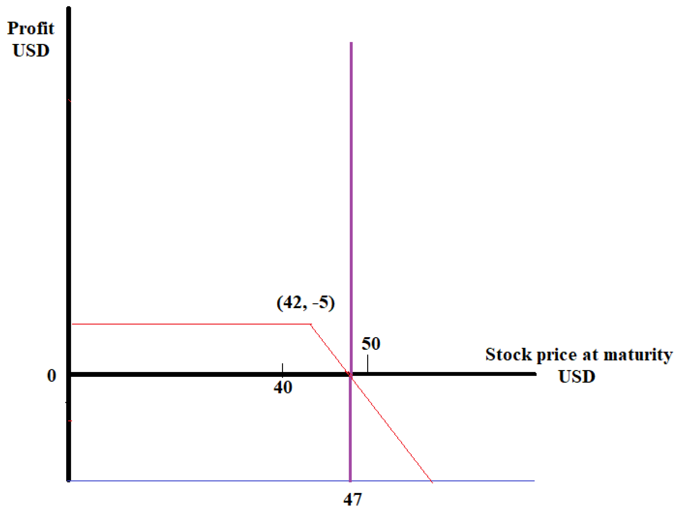
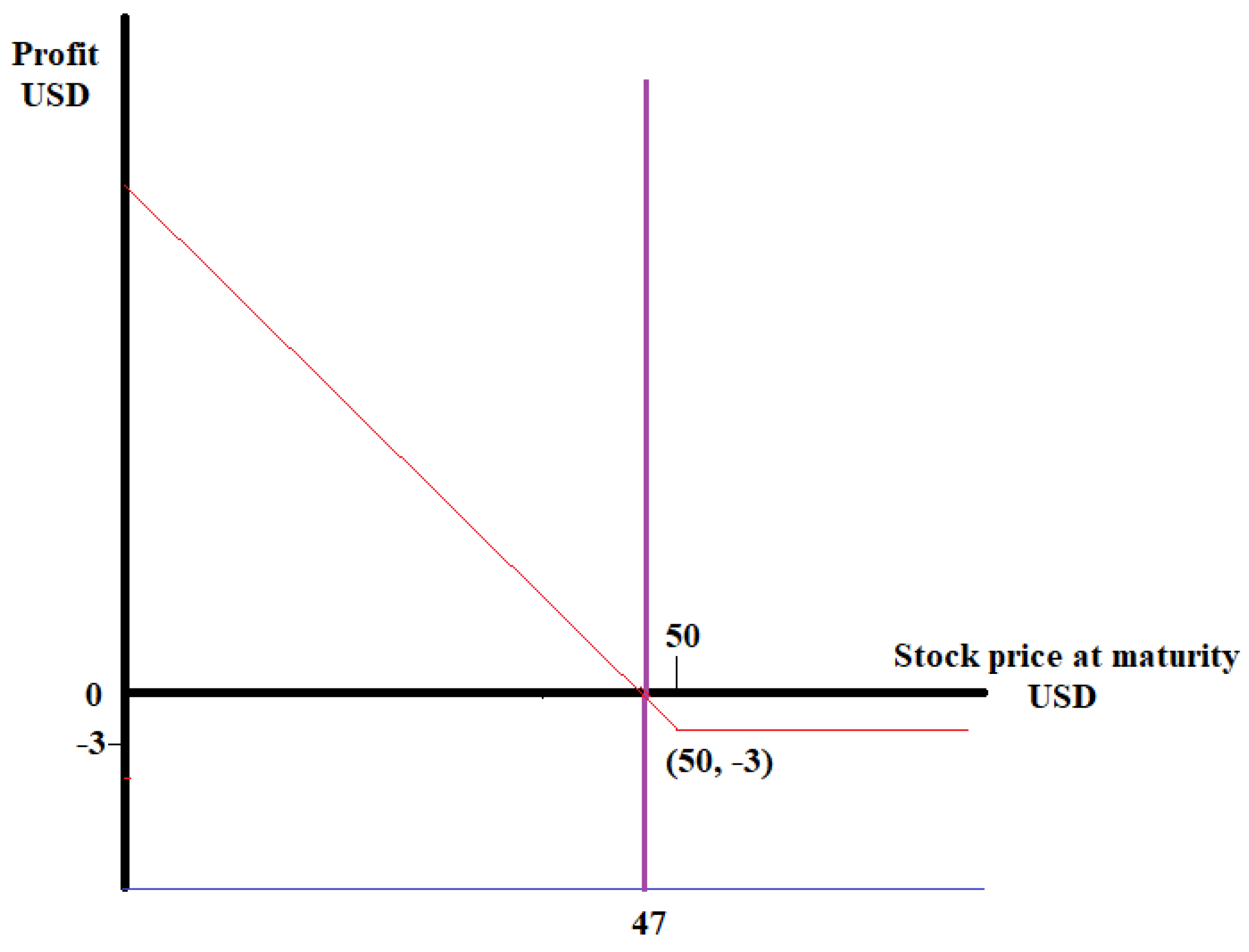
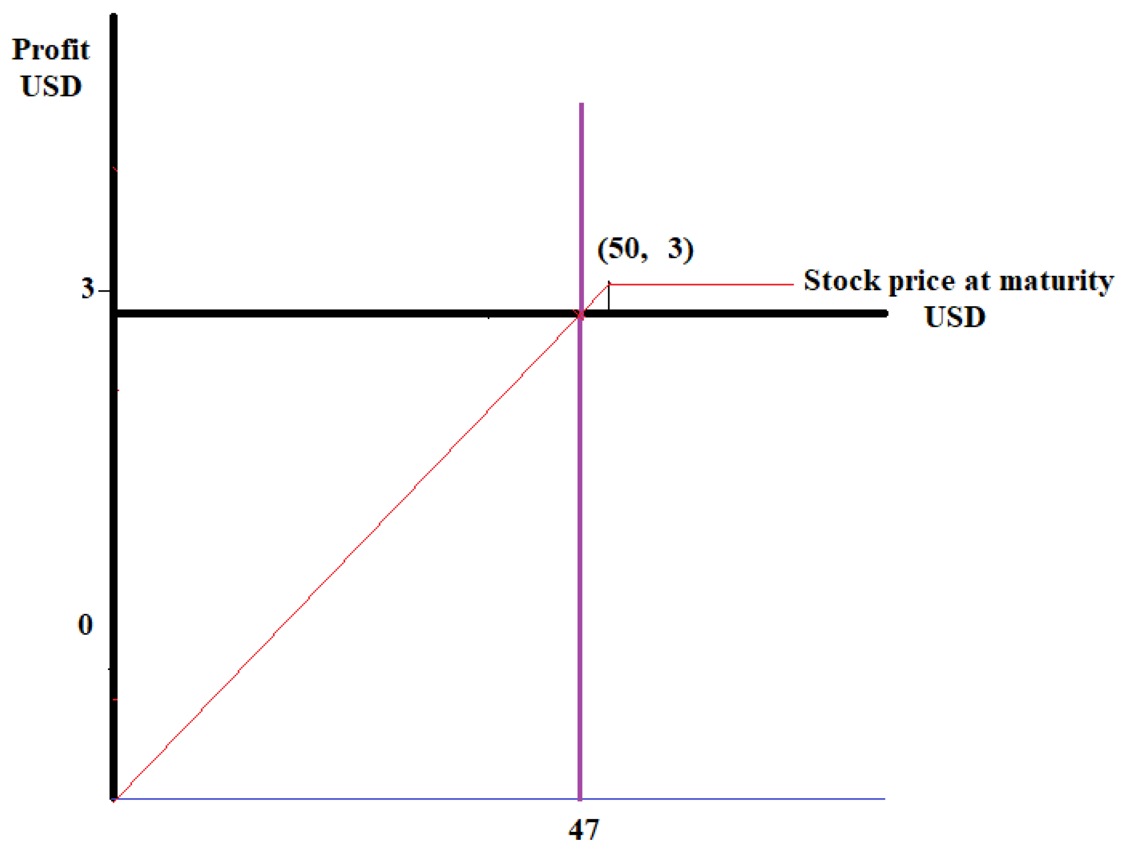
We will develop an example as follows. Imagine that the holder of a call option bought it at USD 5 per share. This operation allows him to decide whether to buy certain amounts of stocks in the future. The price to pay is called the strike price; it is USD 42 per share in this case. If the holder wants to obtain earnings, the stock price must reach a value of more than USD 47 per share. This can be easily visualized because the holder buys the derivative at USD 5. This means that the holder will lose this amount per share. At the same time, the writer of the option earns this amount, making this negotiation a zero-sum game. The profits of the holder of the option can be visualized in Figure 1. From the figure, it is clear that profits begin to be positive when the stock price is larger than USD 47. If the option is a European option, the holder has to wait for the expiration date in order to proceed, the decision to buy will come if the stock price remains higher than the mentioned value. If the option is an American option, it can be exercised at any time, but being rational, this will occur only when the stock price is again larger than USD 47. If the holder finds out that he/she will have negative profits, namely, when the stock price is inferior to USD 47, he/she will not exercise it, and then he/she will lose USD 5 per share. Still, if the stock price at maturity is between USD 42 and USD 47, the holder might decide to exercise the option for reducing losses. In this scenario, whatever the holder earns, the writer loses, and vice versa. This can be seen from Figure 2, which illustrates the possible earnings of the writer of the option. From the present analysis, it is important to remark that in this zero-sum game, there are no limits on the possible profits that the holder can make. On the other hand, the writer’s earnings are limited, as suggested in Figure 2. Another type of option is the put option. This option is the opposite of the call option because it allows the holder the right to sell a certain amount of stocks at a predetermined price. In these situations, the holder is bearish, hoping for the stock prices to be sold to fall. This can be seen from the profits appearing in Figure 3.
Here, the option price is USD 3. Then, at the initial trading, the writer of the option earns this amount of money per share, while the opposite applies to the holder. These details can be seen in Figure 4.
If we analyze the details of Figure 3 and Figure 4, they are the exact reflections of each other, a typical behavior of a zero-sum game. For simplicity, here, we consider a European call option, where the holder can only exercise at maturity. The positive pay-offs for the holder exist when the price of the underlying asset is inferior to USD 47. For asset prices larger than this value, the holder might decide to exercise the right to sell, mainly to minimize losses when appropriate. In this example, the largest possible income for the holder is USD 47. At the same time, due to the zero-sum game nature of the negotiation, the writer will lose anything the holder earns, and vice versa.

3. The Merton–Garman Equation

In this section, we consider the MG financial equation, which is the extension of the BS case, but this time, we consider volatility as a stochastic variable [3,4]. When the option price and volatility are both stochastic variables, then the market is incomplete [15]. Modeling volatility is a big challenge and several approaches have been proposed [23]. However, here, we consider the approach considered in [15], which corresponds to the generic situation. We consider the following set of equations:
d S d t = ϕ S d t + S V R 1 , d V d t = λ + μ V + ζ V α R 2 .
In these equations, volatility is denoted as V = σ 2 . S is just the stock price, as usual. Additionally, ϕ , λ , μ , and ζ are constants or, more accurately, free parameters of the system [24]. The variables R 1 and R 2 , denoting Gaussian noises, correspond to each of the variables under analysis. They are correlated in the following way:
< R 1 ( t ) R 1 ( t ) > = < R 2 ( t ) R 2 ( t ) > = δ ( t t ) = 1 ρ < R 1 ( t ) R 2 ( t ) > .
Here, 1 ρ 1 , and the brackets <   A B   > correspond to the correlation between A and B. The fact that the random noises between both variables are correlated, as seen in Equation (9), suggests—in advance—an important connection between stock prices and the values taken by volatility. This is an important aspect of the MG analysis, which is reflected at the moment of using the gauge principle. Let us now consider a function, f, depending on the stock price, time, and white noise. By using Itô calculus, it is possible to derive the total time derivative of this function as follows:
d f d t = f t + ϕ S f S + ( λ + μ V ) f V + σ 2 S 2 2 2 f S 2 + ρ V 1 / 2 + α ζ 2 f S V + ζ 2 V 2 α 2 2 f V 2 + σ S f S R 1 + ζ V α f V R 2 .
We can now separate the stochastic terms from the non-stochastic ones. The result is as follows:
d f d t = Θ + Ξ R 1 + ψ R 2 .
Here, we define the following:
Ξ = σ S f S , ψ = ζ V α f V , Θ = f t + ϕ S f S + ( λ + μ V ) f V + σ 2 S 2 2 2 f S 2 + ρ V 1 / 2 + α ζ 2 f S V + ζ 2 V 2 α 2 2 f V 2 ,
The notation used here is the same as what was proposed in [15].

3.1. Derivation of the Merton–Garman Equation

The derivation of the MG equation is a very important mathematical exercise. We start by considering two different options, here defined as C 1 and C 2 , on the same underlying security, with strike prices and maturities given by K 1 , K 2 , T 1 , and T 2 , respectively. We can then create a portfolio:
Π = C 1 + Γ 1 C 2 + Γ 2 S .
By using the result (11), we can define the total derivative of the portfolio with respect to time, as follows:
d Π d t = Θ 1 + Γ 1 Θ 2 + Γ 2 ϕ S + Ξ 1 + Γ 1 Ξ 2 + Γ 2 σ S R 1 + ψ 1 + Γ 1 ψ 2 R 2 .
This result is a consequence of identifying f ( t ) = C 1 or f ( t ) = C 2 in Equation (11). Although the market is incomplete in this case, we can create a hedged portfolio that is able to satisfy the condition d Π d t = r Π . The white noise variables, R 1 and R 2 , disappear after imposing the following conditions:
ψ 1 + Γ 1 ψ 2 = 0 , Ξ 1 + Γ 1 Ξ 2 + Γ 2 σ S = 0 .
We can then solve these equations for Γ 1 and Γ 2 . We can now define the parameter, as follows:
β ( S , V , t , r ) = 1 C 1 / V C 1 t + ( λ + μ V ) C 1 S + V S 2 2 2 C 1 S 2 + ρ V 1 / 2 + α ζ 2 C 1 S V + ζ 2 V 2 α 2 2 C 1 V 2 r C 1 = 1 C 2 / V C 2 t + ( λ + μ V ) C 2 S + V S 2 2 2 C 2 S 2 + ρ V 1 / 2 + α ζ 2 C 2 S V + ζ 2 V 2 α 2 2 C 2 V 2 r C 2
The parameter β in the MG equation is defined as the market price volatility risk because the higher its value is, the lower the intention of the investors to risk. Then, the risk of the market is always included in the MG equation. Since volatility is not traded in the market, it is not possible to make a direct hedging process over this quantity [15]. In Ref. [15], it was verified that the value of β is different from zero. With all these arguments, the MG equation is obtained by re-expressing Equation (16) in the following form:
C t + r S C S + ( λ + μ V ) C V + 1 2 V S 2 2 C S 2 + ρ ζ V 1 / 2 + α S 2 C S V + ζ 2 V 2 α 2 C V 2 = r C .
Here, the effects of β appear contained inside the modified parameter, λ , in this equation. This can be seen from the shift, λ λ β , in Equation (17).

3.2. Hamiltonian Form of the Merton–Garman Equation

It has previously been demonstrated that after conducting the corresponding change of variable, the MG equation takes its Hamiltonian form. The change of variable applies to both the price of the stock and the volatility as follows:
S = e x , < x < , σ 2 = V = e y , < y < .
By using these relations, Equation (17) becomes [15]:
C t + r e y 2 C x + λ e y + μ ζ 2 2 e 2 y ( α 1 ) C y + e y 2 2 C x 2 + ρ ζ e y ( α 1 / 2 ) 2 C x y + ζ 2 e 2 y ( α 1 ) 2 C y 2 = r C .
The Schrödinger-like equation is as follows:
C t = H ^ M G C ,
with the MG Hamiltonian defined as follows:
H ^ M G = e y 2 2 x 2 r e y 2 x λ e y + μ ζ 2 2 e 2 y ( α 1 ) y ρ ζ e y ( α 1 / 2 ) 2 x y ζ 2 e 2 y ( α 1 ) 2 y 2 + r .
Exact solutions for the MG equation have been found for the case α = 1 in [15] by using path-integral techniques. The same equation has been solved for the case α = 1 / 2 by using standard techniques of differential equations. The MG equation has two degrees of freedom. Similarly to the BS Hamiltonian, the MG Hamiltonian is also non-Hermitian, meaning it does not preserve information, a characteristic typical of stochastic processes.

3.3. Limitations of the Merton–Garman Equation

The MG equation was derived in order to improve the limitations, related to volatility, of the BS equation. Inside the BS scenario, volatility is a parameter that we have to estimate. Instead, the MG equation introduces volatility as a stochastic variable [2,3,4]. Yet, the MG equation has certain limitations. The most significant limitation of the MG equation is that its solutions are difficult to derive, except for some specific combinations of parameters or under some perturbative methods [3,4,25]. Since volatility is a stochastic variable in this case, and it is not traded in the market, there are not enough instruments to perfectly hedge against volatility. For this reason, the MG equation requires an additional parameter β ( S , V , t , r ) introduced in Equation (16) and explained previously. The parameter β itself, just mentioned, is difficult to estimate empirically [15] but it is clear that it must be non-zero. The biggest difficulty in explicitly solving the MG equation comes from the dependence on stock price volatility. However, in the case where ρ = 0 , there is no correlation between the stock price and stochastic volatility, as can be seen in Equation (9). Then, in this limit, the stock price and stochastic volatility are independent, and then an explicit solution for the MG equation can be found [15]. Merton demonstrated that such a solution is equivalent to the result of the BS equation, but instead of using stochastic volatility as a variable, it is taken by the average value [4]. Then, the solutions for the option price can be expressed as follows:
C = 0 S N ( d + ( V ¯ ) K e r τ N ( ( d ( V ¯ ) ) P M ( V ¯ ) d V ¯ V ¯ ,
with the average volatility expressed as follows:
V ¯ = 1 τ t T d t V ( t ) .
In Equation (22), P M is the probability distribution for the mean value volatility defined in Equation (23). Additionally, the function d + ( V ¯ ) is defined as follows:
d ± = L n ( S / K ) + τ ( r ± 1 2 V ¯ ) V ¯ τ ,
with K representing the strike price. Certain examples applying these formulas were developed in [15]. For cases where ρ 0 , the situation becomes very complicated, limiting the MG equation to a few approximations.

4. Symmetries of the Black–Scholes Hamiltonian

The symmetries of the Black–Scholes Hamiltonian were analyzed in [5,6]. The symmetries we care about are those related to changes in stock prices. We define the operator, U = e ω θ ( x ) , which defines the changes in the system with respect to stock prices. The operator, U, in this case, is non-unitary because the processes in the stock market are basically stochastic, and unitarity is not respected at all. We focus on local transformations, where θ ( x ) is a parameter that depends on x, which is a function of the stock prices as can be seen from Equation (18). With the BS Hamiltonian defined as H ^ B S , the operator, U, would be a symmetry of the system if the relation [ H ^ B S , U ] = 0 were satisfied. However, it was demonstrated in [5] that U is not a local symmetry of the system represented by the BS equation. This means that the commutator satisfies the following relation:
[ H ^ B S , U ] 0 .
The transformation, represented by U, becomes a symmetry when we include a gauge field, which turns out to be stochastic volatility [5]. Let us analyze this issue in more detail. If we operate with U over the Hamiltonian, H ^ B S , we obtain the following:
H ^ B S H ^ B S + σ 2 ω ( 1 + ω ) 2 θ ( x ) x 2 + σ 2 ω θ ( x ) x x + ω 1 2 σ 2 r θ ( x ) x .
Then, the local symmetry under changes in stock prices is not satisfied by the standard BS equation. If we want to restore this symmetry, we need to introduce stochastic volatility with its corresponding transformation under local price changes, compensating for any variation in the Hamiltonian H ^ B S under the same transformation. Since volatility acts as a gauge field, the ordinary derivative is replaced by a covariant derivative, defined as follows:
x x + p ^ y .
While p ^ x = x is the “momentum” associated with the stock prices, p ^ y is the momentum associated with stochastic volatility. Then the extended BS Hamiltonian is able to satisfy the local symmetry under the changes U = e ω θ ( x ) , defined as follows:
H ^ B S H ^ g a u g e = σ 2 2 p ^ x p ^ y p ^ x + p ^ y + 1 2 σ 2 r p ^ x + p ^ y + r .
Here, we define the extended BS Hamiltonian as the gauge Hamiltonian, as indicated by the subscript, g a u g e , appearing in Equation (28). It has been proven that this Hamiltonian is a special case of the MG Hamiltonian, as defined in Equation (21) [5]. The Hamiltonian (28) can be expressed as follows:
H ^ g a u g e = σ 2 2 p ^ x 2 + 1 2 σ 2 r p ^ x σ 2 2 p ^ y 2 σ 2 p ^ x p ^ y + 1 2 σ 2 r p ^ y + r ,
after conducting the corresponding expansion. Gauge invariance is guaranteed if the following conditions are satisfied:
θ x 2 = ω 1 + ω θ y 2 , θ x p ^ x = θ y p ^ y , θ x + θ y 4 2 θ x y = 2 r σ 2 θ x + θ y .
Under these conditions, Equation (29) represents the MG Hamiltonian, when the following relations between the parameters are satisfied:
ζ 2 = e 2 y α 3 2 , ρ ζ = e y α 3 2 , r = λ e y + μ .
These relations represent a family of Hamiltonians consistent with the MG one. Relation (31) reduces volatility to one additional parameter, unless certain combinations of the free parameters have stochastic nature. The conditions (31) are very restrictive, and in this paper, we omit them. Our Hamiltonian, defined in Equation (29), together with condition (30), is not necessarily the MG Hamiltonian but rather a different Hamiltonian, which is locally equivalent to the BS Hamiltonian. If we solve the second equation from the group of equations in (30), and we use the first equation from the same group, we obtain the following:
p ^ x p ^ y = θ y θ x = ± ω 1 + ω .
For ω > > 1 , this means that p ^ x ± p ^ y . No matter the value taken by the parameter, ω , the proportionality between the absolute value of the momentum associated with changes in stock prices and the momentum related to changes in volatility means that if we consider that the price of an option increases with volatility, namely, p ^ y > 0 , then the price of the option can increase or decrease with the price of the related stock. We conclude that the positive sign in Equation (32) is ideal for the holders of a call option, while the negative sign is the ideal scenario for the holders of the put options. This is the case because call options are always increasing in price with the stock price, while the opposite applies to the put options. No matter what option we consider, an increase in volatility is equivalent to an increase in the price of the option. This is consistent with stock market pattern observations. Finally, the last relation appearing in the group in Equation (30) leads to the following:
1 + p ^ x p ^ y 4 2 θ x y θ x = 2 r σ 2 1 + p ^ x p ^ y .
This result is trivial when 2 r = σ , which is precisely the case where the Hamiltonian (7) becomes Hermitian, ensuring that the information in the options market is preserved. Then, Equation (33) provides a way to determine the conditions under which information is not preserved in the stock market. Equation (33) can be expressed as follows:
1 + p ^ x p ^ y = 4 σ 2 ( σ 2 2 r ) 2 θ x y θ x .
As we can see, the condition σ 2 = 2 r requires 2 θ x y = 0 in order to keep the left-hand side of Equation (34) finite.

Local Equivalence of the Merton–Garman and Black–Scholes Equations: The Gauge Principle

For the family of MG Hamiltonians that satisfy local symmetry under price changes, namely, the Hamiltonian (29), the momentum associated with volatility—acting as a gauge field—is responsible for restoring the system’s symmetry under local price changes. The gauge principle suggests that the family of MG Hamiltonians, consistent with the gauge principle, is locally equivalent to the BS Hamiltonian. In other words, the MG equation—consistent with the gauge principle—is locally equivalent to the BS equation. This means that if we switch off the momentum associated with volatility p ^ y , we will recover the BS equation. This is a trivial task that is easy to verify. The key point of this section is the interpretation behind switching off the momentum associated with stochastic volatility. The condition to analyze is as follows:
H ^ g a u g e = H ^ M G p ^ y C 0 H ^ B S .
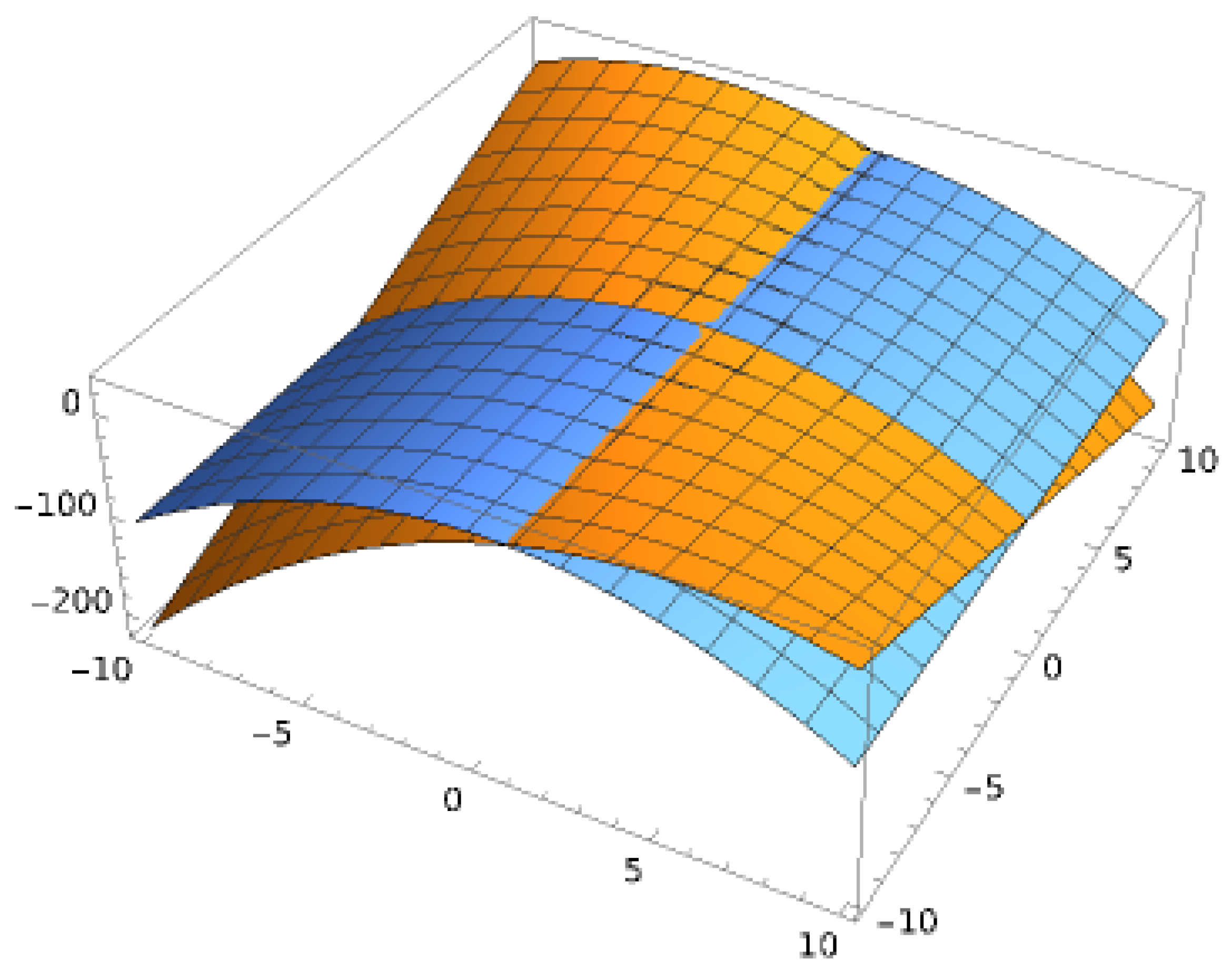
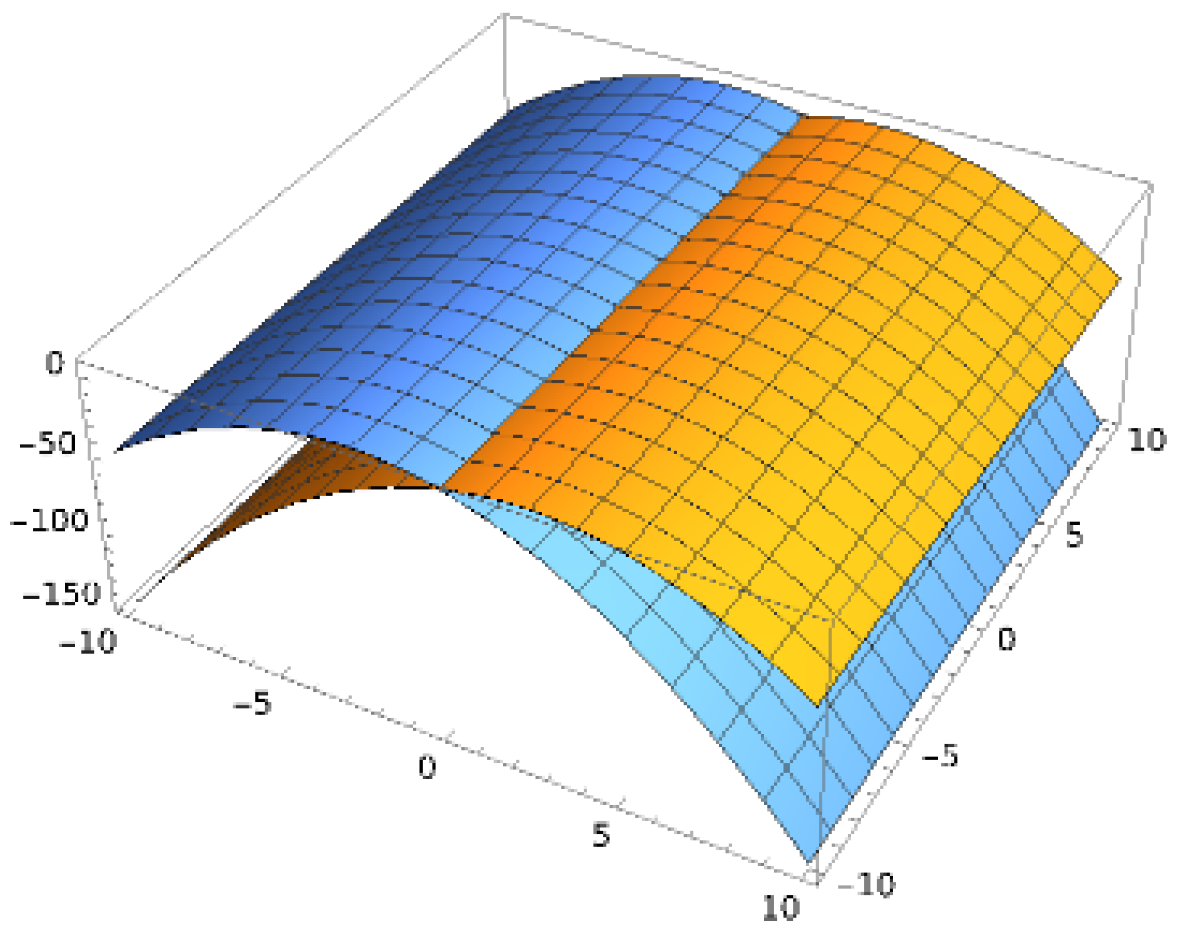
The condition p ^ y C 0 means that any variations in the prices of the options due to changes in volatility are completely ignored when we consider the BS limit. The graphic representation of this situation can be seen in Figure 5. We can perceive volatility as a field generating some “weight” over the option prices. This weight causes the option prices to deviate from the usual path they would follow if the momentum associated with volatility were suppressed. When the momentum associated with volatility vanishes, we can see from the figure that the BS Hamiltonian (blue plot) intersects with the MG Hamiltonian (yellow figure), because—in this limit—both Hamiltonians are the same.
From the same figure, it can be seen that, in general, the MG Hamiltonian does not match the BS Hamiltonian. Equality occurs when p ^ y = 0 , as mentioned, but also for the non-trivial case, where p ^ y 0 , provided that the eigenvalues of p ^ x satisfy the following:
p ^ x | C > + 1 2 p ^ y | C > = 1 2 r σ 2 | C > .
Note that this relation becomes trivial on the right-hand side when σ 2 = 2 r , which is precisely the condition for the options market to preserve the information based on the Hermiticity condition of the BS Hamiltonian. When this occurs, we then obtain the following relation:
2 p ^ x = p ^ y ,
which is only valid when an increase in the price of an option is related to a decrease in the price of the underlying stock (bearish behavior). The result (36) is surprising because this means that even when there is a non-trivial value of stochastic volatility (taken as a variable), the BS Hamiltonian can be recovered from the gauge Hamiltonian, provided that the combination p ^ x + 1 2 p ^ y obeys the equality in (36). Note the behavior of the BS Hamiltonian in the Figure 6.

5. The Martingale Condition with Stochastic Volatility

In [5,6], it was proven that some relationships between the field associated with stock prices and the field corresponding to stochastic volatility emerge when we consider the vacuum or martingale condition in the MG scenario. The martingale is then defined as follows:
H ^ M G e x + y = H ^ M G S ( x , y , t ) = 0 .
For the non-trivial behavior of stochastic volatility ( p ^ y 0 ), this condition corresponds to a martingale condition if the following result is satisfied:
λ + e y μ + ζ 2 2 e 2 y ( α 1 ) + ρ ζ e y ( α 1 / 2 ) = 0 ,
It was demonstrated in [5,6] that the combination of Equations (31) and (39) brings out the following simple relation:
e 2 y + μ e y + λ = 0 ,
which can be easily solved, finding some specific relation between the volatility prices and some of the free parameters ( μ and λ ) of the system. The relation (40) is valid at the equilibrium (martingale) state of the system because its origin comes from Equation (38). The same relation suggests that at the equilibrium condition, volatility depends on some free parameters of the MG Hamiltonian. Outside the equilibrium, naturally, the condition (40) is not necessarily satisfied. Now, we can analyze the martingale condition for the gauge Hamiltonian defined in Equation (29), without the restrictions of the MG case. In other words, we will now generalize the situation for cases where it is also possible to have H ^ g a u g e H ^ M G . Here, we remark that H ^ g a u g e covers a more general case compared to the restrictive MG Hamiltonian. From the Hamiltonian (29), we can define the martingale condition as follows:
H ^ g a u g e | S > = 0 .
Let us take the martingale state as a series expansion | S > = n ϕ n = n ( ϕ x ϕ y ) n , as suggested in [6]. In such a case, it is possible to demonstrate that the martingale condition gives the following result:
ϕ x v a c = ϕ r v a c .
This simply suggests that the martingale condition emerges when the variations in the prices of the option, due to changes in stock prices, equal the variations in the prices of the options due to changes in volatility. This means that the market equilibrium can be achieved with non-trivial values of volatility, as long as the condition (42) is satisfied. This surprising result is a natural consequence of the gauge principle. Note that this condition was obtained before when ω > > 1 in Equation (32). Then, the gauge principle suggests important relational connections between stock prices and the values associated with market volatility.

6. Interpretations from the Perspective of Physical Systems

In this paper, we demonstrated that the gauge principle is able to unify the Black–Scholes and Merton–Garman equations. Furthermore, a more general Hamiltonian, without the constraints imposed by the MG equation, emerges. One interesting aspect of the gauge formulation is that stochastic volatility is the gauge field that we have to introduce to restore the local invariance over changes in stock prices. In this section, we make an analogy between this case and the gauge symmetries observed in physics. We will explore two analogies. The first one is where manifolds are considered. This part involves the natural connection between special and general relativity. In fact, special and general relativity are two theories locally equivalent [7]. The second analogy, which we will explore, is the gauge formulation of electrodynamics [8,26]. In this case, we will observe how the photon field emerges as the gauge field that restores local symmetry—a role played by stochastic volatility in our formulation.

6.1. Analogy with Relativity

If we focus our attention on manifolds, this analogy can be understood by considering both general relativity and special relativity. In this case, both theories are locally equivalent. Then, when we gauge the coordinate system in special relativity, we obtain general relativity. In other words, the source of gravity is the gauge field capable of restoring local symmetry under the coordinate transformation. This is analogous to the appearance of volatility, which emerges as the variable restoring the local symmetry under changes in prices for the BS equation. To understand this analogy in deeper detail, we have to analyze and compare the global and local structures of the flat spacetime (Minkowski) and the curved spacetime (spacetime with gravity). For simplicity, we will take the Schwarzschild solution as the solution representing the curved spacetime. The respective metrics are as follows:
d s M 2 = d t 2 + d r 2 = r 2 d Ω 2 ,
for the Minkowskian metric, and
d s S 2 = 1 Φ d t 2 + 1 Φ 1 d r 2 = r 2 d Ω 2 ,
for the Schwarzschild metric [7]. Here, Φ is just the deviation from the flatness condition for this metric. As soon as gravity disappears, Φ 0 , and the metric (44) becomes equivalent to the Minkowski metric (43). Here, we use manifolds with a metric, but it is important to note that the existence of a manifold is independent of the metric [27]. It is not necessary to use the Einstein equations to understand this part; instead, we will focus on the geodesic equations. The general form of the geodesic equations is as follows:
d 2 x μ d τ 2 + Γ ρ σ μ d x ρ d τ d x σ d τ .
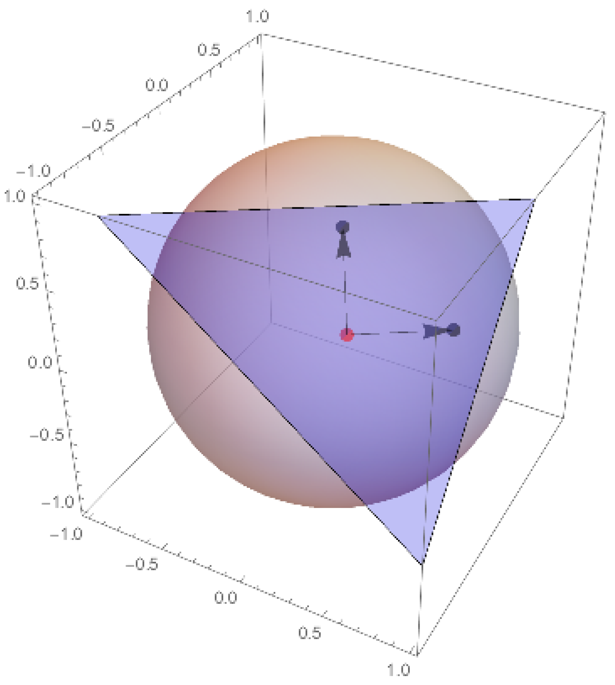
These equations mark the shortest trajectory of a test particle moving along a manifold. They emerge from the Lagrangian density, g μ ν d x μ d τ d x ν d τ . Then, Γ ρ σ μ 0 in Equation (45), and we have a non-trivial manifold, here represented by simplicity as a sphere in Equation (45). Γ ρ σ μ is a derivative function of the potential functions, Φ , which appear in the metric (44). Still, locally, the gravitational effects vanish, and then Γ ρ σ μ = 0 . This is the famous equivalence principle, which allows general relativity to recover special relativity locally [7]. If we make an analogy, the BS equation is locally equivalent to the MG equation and, more generally, to the system represented by the gauge Hamiltonian in Equation (28), because stochastic volatility becomes a constant locally (this means that p ^ y vanishes locally in Equation (28)). In such a case, the effects of volatility are translated in such a case to a parameter ( σ in Equation (7)), which has to be fixed. The Figure 7 shows a tangent plane which would be analogue to the BS equation, while the MG equation would correspond to the non-trivial case.

6.2. Analogy with Quantum Electrodynamics

The photon field emerges as the gauge field capable of restoring local symmetry in some very well-known cases [8,26]. As a basic example, we have a massive scalar field, ϕ , represented by the Klein–Gordon Lagrangian, defined as follows:
£ = ( μ + i e A μ ) ϕ ( μ + i e A μ ) ϕ * m 2 ϕ ϕ * 1 4 F μ ν F μ ν .
Here, A μ is the photon field, represented by a vector. This photon field helps to restore the local symmetry under the following changes:
ϕ e i Λ ( x ) ϕ .
Note that if we introduce the scalar field transformed as proposed in Equation (47) into Equation (46), then only the derivative terms are affected. The only way to restore invariance under these transformations is by introducing the photon field, A μ , which restores local symmetry as far as the photon field transforms, in such a way as to cancel any possible variations arising in the Lagrangian (46) after applying the local transformation (47) over the field ϕ . The transformation conducted over A μ does not affect the term 1 4 F μ ν F μ ν . It is standard practice to define a covariant derivative that includes the gauge field, such as D μ = μ + i e A μ , such that we can express the Lagrangian (46) in a compact form. The covariant derivative by itself has a meaning; it shows the fact that the variations in the field, ϕ , require corrections due to the fact that a good definition of the derivative along a non-trivial manifold requires a parallel transport of the initial field, ϕ , toward the same point where the variation of ϕ is evaluated. This is the case because the axis orientations change point to point in these cases due to the presence of the photon field [26]. From the Lagrangian (46), after including higher-order terms, certain interesting phenomena involving spontaneous symmetry breaking [8,9,10,11,12,13,14], such as superconductivity [26]. From the perspective of the Black–Scholes equation, stochastic volatility, or more specifically, the momentum associated with it, p ^ y , plays the exact same role as the photon field in the gauge theory related to the Lagrangian (46). Another example is quantum electrodynamics (QED), where the photon field emerges as the gauge field, which restores the local symmetry of the Lagrangian [26]. The QED Lagrangian is defined as follows [8]:
£ Q E D = ψ ¯ ( i γ μ D μ m ) ψ 1 4 F μ ν F μ ν .
Here, again, F μ ν F μ ν is an invariant term, which contains the kinetic terms for the photon field A μ [8]. In this case, the covariant derivative is defined in the same way as the Lagrangian (46). Here, again, the photon field plays the role of a gauge field, restoring the local symmetry of the Lagrangian. For the BS and MG cases, the momentum associated with volatility plays this role.

7. Alternative Models: The Origin of Stochastic Volatility

As we have analyzed in this paper, stochastic volatility emerges from imposing invariance under local changes in the stock prices. This means that, evidently, stochastic volatility has a close relationship with asset prices. However, this relation is not arbitrary since it has to be constrained to respect the mentioned invariance. Still, several models have been proposed to analyze the relationships between option prices, stock prices, and stochastic volatility within the market. In what follows, we will mention a few models that address local aspects of stochastic volatility.

7.1. The Bachelier Model

The stochastic volatility model started with Louis Bachelier in 1900 [28]. This work allows the assets to take negative prices, which was long regarded as a limitation. However, during extreme crises, like COVID-19, oil prices fell catastrophically, and by April 2020, the price of oil futures contracts reached negative values—something without any prior precedent [29]. Similar effects were seen during the 2008 crisis. This type of effect resurrected the Bachelier model. This model assumes that the forward price, F t , at maturity, T, of an asset at time t, follows the condition:
d F t = σ t d W t .
Here, W t is the Brownian motion under the T-forward measure. Inside this model, the price for the call option is defined as follows:
C N ( k ) = ( F 0 K ) N ( d N ) + σ N T n ( d N ) , d N = F 0 K σ N T .
Here, C N denotes the undiscounted price of the option, K denotes the strike price, and T denotes maturity. Additionally, n ( d N ) denotes the probability density function for the standard normal distribution, while N ( d N ) denotes the cumulative distribution function for the same distribution. At the money, the price of the option is simplified as follows:
C N ( F 0 ) = σ N T 2 π .
Here, it is easy to solve for volatility.

7.2. The Displaced Black–Scholes Model

The displaced BS model enables the possibility of having negative asset prices and negative volatility skew [29,30,31]. Inside this model, the call option price is as follows:
C D ( K ) = D ( F 0 ) N ( d 1 D ) D ( K ) N ( d 2 D ) β .
Here, the function N ( d 1 D , 2 D ) is the cumulative normal distribution for the corresponding variable. d 1 D , 2 D is defined as follows:
d 1 D , 2 D = D ( F 0 ) / D ( K ) β σ D T ± β σ D T 2 .
This model could be represented by the same Hamiltonian of the form defined in Equation (7), considering that the price of the option, C, is displaced in agreement with a general expression, as follows:
D ( C ) = C B S + M .
Here, M is a function of certain parameters inside the model. Then, in essence, the MG equation can also be derived from the displaced BS model, but taking into account the shifts on the prices of the options.

7.3. General Analysis of Alternative Models

In general, all the alternative models to the BS equation can be expressed with a Hamiltonian of the following form:
H ^ = σ 2 2 2 x 2 + 1 2 σ 2 r x + r + V ^ ( x , σ , r ) .
These extensions can work very well for models in which the prices of the options are shifted by parameters that are independent of the prices. On the other hand, the most general modification of the Hamiltonian that describes the prices of options takes the form of the following expression:
H ^ = σ 2 2 x 2 + 1 2 σ 2 r x + r + V ^ ( x , σ , r ) ,
where x is defined as a covariant derivative, which includes not only the ordinary derivative term but also the gauge field, compensating for any possible shift in the model. Then, in general, we have the following:
x = x + A y ,
with A y representing the gauge field. The Hamiltonian (56) is the most general Hamiltonian, covering not only the BS and MG models, but also any other possible shift and/or extension of these models.

8. Conclusions

In this paper, we demonstrate the power of the gauge principle when it is applied to the options market through the BS Hamiltonian. First, the gauge principle shows that the MG equation is locally equivalent to the BS equation. However, the Hamiltonian obtained by imposing gauge symmetry (gauge Hamiltonian) under price changes is more general than the MG Hamiltonian and it leads to remarkable results. It suggests, for example, that there is a martingale condition when the variations in the prices of the options, with respect to the stock price changes, are equal to the changes in the prices of the options with respect to changes in volatility. The gauge principle suggests that the gauge Hamiltonian yields the same results as the BS Hamiltonian when either of the following two conditions is satisfied: (1) The momentum associated with volatility is zero; (2) a specific combination of the momentum associated with stock prices and the momentum associated with volatility is achieved, as Equation (36) suggests. Future analysis involving the importance of the gauge principle on the options market is under analysis. This paper demonstrates that the concepts of symmetry and gauge theory are not only important in physics, which bring out several important results [9,10,11,12,13,14], but are also important for understanding the most fundamental principles behind the options market [5,6]. In such a case, the momentum associated with stochastic volatility p ^ y , plays the role of the gauge field restoring the local symmetry under price changes. Drawing an analogy with some physical theories, it has been found that the momentum associated with volatility is analogous to the photon field in QED and the gravitational connections in general relativity [7,8,26]. Then, we conclude that the BS equation is locally equivalent to the MG equation and the system represented by the gauge Hamiltonian (28). In other words, locally, p ^ y = 0 operates similarly to how gravity can be shuttled down locally ( Φ = 0 under the equivalence principle) and how the photon field can be locally nullified in QED [8,26]. In future papers, we will verify other derivative instruments by looking into the symmetries that they must satisfy globally and locally. By imposing local symmetry, we can then find the corresponding gauge fields restoring local invariance. The role of these gauge fields in different scenarios is extremely important. Finally, it is important to note that possible defaults on the options normally generate changes in the differential dynamics of the market [32,33,34]. Such changes are reflected in the possible equilibrium conditions. In these scenarios, the local equivalence between the BS and MG equations is valid but new symmetry conditions and/or new gauge fields might emerge. These scenarios will be analyzed in future papers. Similar situations that we find in other scenarios, involving generalizations of the BS scenario, as well as infinite activity jumps [35,36,37], will also be a part of a future paper involving the gauge principle. Finally, we must note that the gauge Hamiltonian proposed in this paper has the same limitations as the MG Hamiltonian, given the fact that they are equivalent to each other. The most general Hamiltonian, able to cover several models, is defined by Equation (56). In fact, the introduction of the gauge field is always necessary when we have to define systems where local transformations become symmetries. This method brings out several models inside. Further research will be necessary for analyzing the Hamiltonian (56) in more general scenarios.

Funding

This research received no external funding.

Data Availability Statement

No new data were created or analyzed in this study. Data sharing is not applicable to this article.

Acknowledgments

The author would like to thank Taksu Cheon from the Kochi University of Technology for hospitality and support during the research visit and presentation carried out at this institution in July 2024. Special thanks go out to Taksu Cheon who encouraged the writing of this paper.

Conflicts of Interest

The author declares no conflicts of interest.

References

  1. Black, F.; Scholes, M. The pricing of Options and Corporate Liabilities. J. Political Econ. 1973, 81, 637. [Google Scholar] [CrossRef]
  2. de Weert, F. An Introduction to Options Trading; John Wiley and Sons, LTD: Hoboken, NJ, USA, 2006; ISBN-13 978-0-470-02970-1 (PB); ISBN-10 0-470-02970-6 (PB). [Google Scholar]
  3. Merton, R.C. The theory of rational Option Pricing. Bell J. Econ. Manag. Sci. 1973, 4, 141–183. [Google Scholar] [CrossRef]
  4. Merton, R.C. Option pricing when underlying stock returns are discontinous. J. Financ. Econ. 1976, 3, 125. [Google Scholar] [CrossRef]
  5. Arraut, I. Gauge symmetries and the Higgs mechanism in Quantum Finance. arXiv 2023, arXiv:2306.03237. [Google Scholar] [CrossRef]
  6. Arraut, I.; Au, A.; Tse, A.C. Spontaneous symmetry breaking in quantum finance. Europhys. Lett. 2020, 131, 68003. [Google Scholar] [CrossRef]
  7. Carrol, S. Spacetime and Geometry: An Introduction to General Relativity; Addison-Wesley: San Francisco, CA, USA, 2019; ISBN 978-0-8053-8732-2. [Google Scholar]
  8. Peskin, M.E.; Schroeder, D.V. An Introduction to Quantum Field Theory; CRC Press; Taylor and Francis Group: Boca Raton, FL, USA, 2018. [Google Scholar]
  9. Glashow, S. The renormalizability of vector meson interactions. Nucl. Phys. 1959, 10, 107. [Google Scholar] [CrossRef]
  10. Salam, A.; Ward, J.C. Weak and electromagnetic interactions. Nuovo C. 1959, 11, 568–577. [Google Scholar] [CrossRef]
  11. Weinberg, S. A Model of Leptons. Phys. Rev. Lett. 1957, 19, 1264–1266. [Google Scholar] [CrossRef]
  12. Arraut, I. The origin of the mass of the Nambu–Goldstone bosons. Int. J. Mod. Phys. A 2018, 33, 1850041. [Google Scholar] [CrossRef]
  13. Arraut, I. The Nambu-Goldstone theorem in non-relativistic systems. Int. J. Mod. Phys. A 2017, 32, 1750127. [Google Scholar]
  14. Arraut, I. The Quantum Yang Baxter conditions: The fundamental relations behind the Nambu-Goldstone theorem. Symmetry 2019, 11, 803. [Google Scholar] [CrossRef]
  15. Baaquie, B.E. Quantum Finance: Path Integrals and Hamiltonians for Options and Interestrates; Cambridge University Press: Cambridge, UK, 2004; pp. 52–75. [Google Scholar]
  16. Bichteler, K. Stochastic Integration with Jumps, 1st ed.; Cambridge University Press: Cambridge, UK, 2002; ISBN 0-521-81129-5. [Google Scholar]
  17. Cohen, S.; Elliott, R. Stochastic Calculus and Applications, 2nd ed.; Birkhaueser: Berlin, Germany, 2015; ISBN 978-1-4939-2867-5. [Google Scholar]
  18. Kleinert, H. Path Integrals in Quantum Mechanics, Statistics, Polymer Physics, and Financial Markets, 4th ed.; World Scientific (Singapore): Singapore, Paperback Fifth Edition Available Online: PDF-Files, with Generalizations of Itô’s Lemma for Non-Gaussian Processes; ISBN 981-238-107-4. Available online: https://www.amazon.com/Integrals-Quantum-Mechanics-Statistics-Financial/dp/9812700080 (accessed on 11 March 2025).
  19. Rehman, M.Z.; Karimullah, K. Black swan events and stock market behavior in Gulf countries: A comparative analysis of financial crisis (2008) and COVID-19 pandemic. Arab Gulf J. Sci. Res. 2024, 42, 805–824. [Google Scholar] [CrossRef]
  20. Al-Raeei, M. Numerical simulation of the force of infection and the typical times of SARS-CoV-2 disease for different location countries. Model. Earth Syst. Environ. 2022, 8, 1443–1448. [Google Scholar] [CrossRef]
  21. Khan, N.; Ahmad, Z.; Ahmad, H.; Tchier, F.; Zhang, X.Z.; Murtaza, S. Dynamics of chaotic system based on image encryption through fractal-fractional operator of non-local kernel. Aip Adv. 2022, 12, 055129. [Google Scholar] [CrossRef]
  22. Griffiths, D.J. Introduction to Quantum Mechanics; Prentice Hall: Upper Saddle River, NJ, USA, 1995. [Google Scholar]
  23. Heston, S.L. A Closed-Form Solution for Options with Stochastic Volatility with Application to Bond and Currency Options. Rev. Financ. Stud. 1993, 6, 327. [Google Scholar] [CrossRef]
  24. Baldwin, R.; Taglioni, D. Trade effects of the euro: A comparison of estimators. J. Econ. Int. 2007, 22, 780–818. [Google Scholar] [CrossRef]
  25. Calmet, X.; Shaw, N.W. An analytical perturbative solution to the Merton Garman model using symmetries. J. Futur. Mark. 2020, 40, 3–22. [Google Scholar] [CrossRef]
  26. Ryder, L.H. Quantum Field Theory, 2nd ed.; Cambridge University Press: Cambridge, UK, 1996. [Google Scholar]
  27. Lee, J.M. Introduction to Topological Manifolds, 1st ed.; Springer: Berlin/Heidelberg, Germany, 2000. [Google Scholar]
  28. Bachelier, L. Theorie de la Speculation. Ann. Sci. L’Ecole Norm. Super. 1990, 17, 21–88. [Google Scholar] [CrossRef]
  29. Choi, J.; Kwak, M.; Wen Tee, C.; Wang, Y. A Black–Scholes user’s guide to the Bachelier model. J. Futur. Mark. 2022, 42, 959–980. [Google Scholar] [CrossRef]
  30. Rubinstein, M. Displaced Diffusion Option Pricing. J. Financ. 1983, 38, 213–217. [Google Scholar] [CrossRef]
  31. Joshi, M.S.; Rebonato, R. A displaced-diffusion stochastic volatility LIBOR market model: Motivation, definition and implementation. Quant. Financ. 2003, 3, 458–469. [Google Scholar] [CrossRef]
  32. Vasquez, A.; Xiao, X. Default Risk and Option Returns. 2020. Available online: https://ssrn.com/abstract=2667930 (accessed on 11 March 2025).
  33. Marzilli Ericson, K.M. When consumers do not make an active decision: Dynamic default rules and their equilibrium effects. Games Econ. Behav. 2020, 124, 369–385. [Google Scholar] [CrossRef]
  34. Yang, H.; Luo, S. A dark side to options trading? Evidence from corporate default risk. Rev. Quant. Financ. Account. 2023, 60, 531–564. [Google Scholar] [CrossRef]
  35. Zaevski, T.S.; Kim, Y.S.; Fabozzi, F.J. Option pricing under stochastic volatility and tempered stable Levy jumps. Int. Rev. Financ. Anal. 2014, 31, 104–108. [Google Scholar] [CrossRef]
  36. Zaevski, T.S.; Kounchev, O.; Savov, M. Two frameworks for pricing defaultable derivatives. Chaos Solitons Fractals 2019, 123, 309–319. [Google Scholar] [CrossRef]
  37. Bates, D.S. Jumps and Stochastic volatility: Exchange Rate Processes Implicity in Deutsche Mark Options. Rev. Financ. Stud. 1996, 9, 69–107. [Google Scholar] [CrossRef]
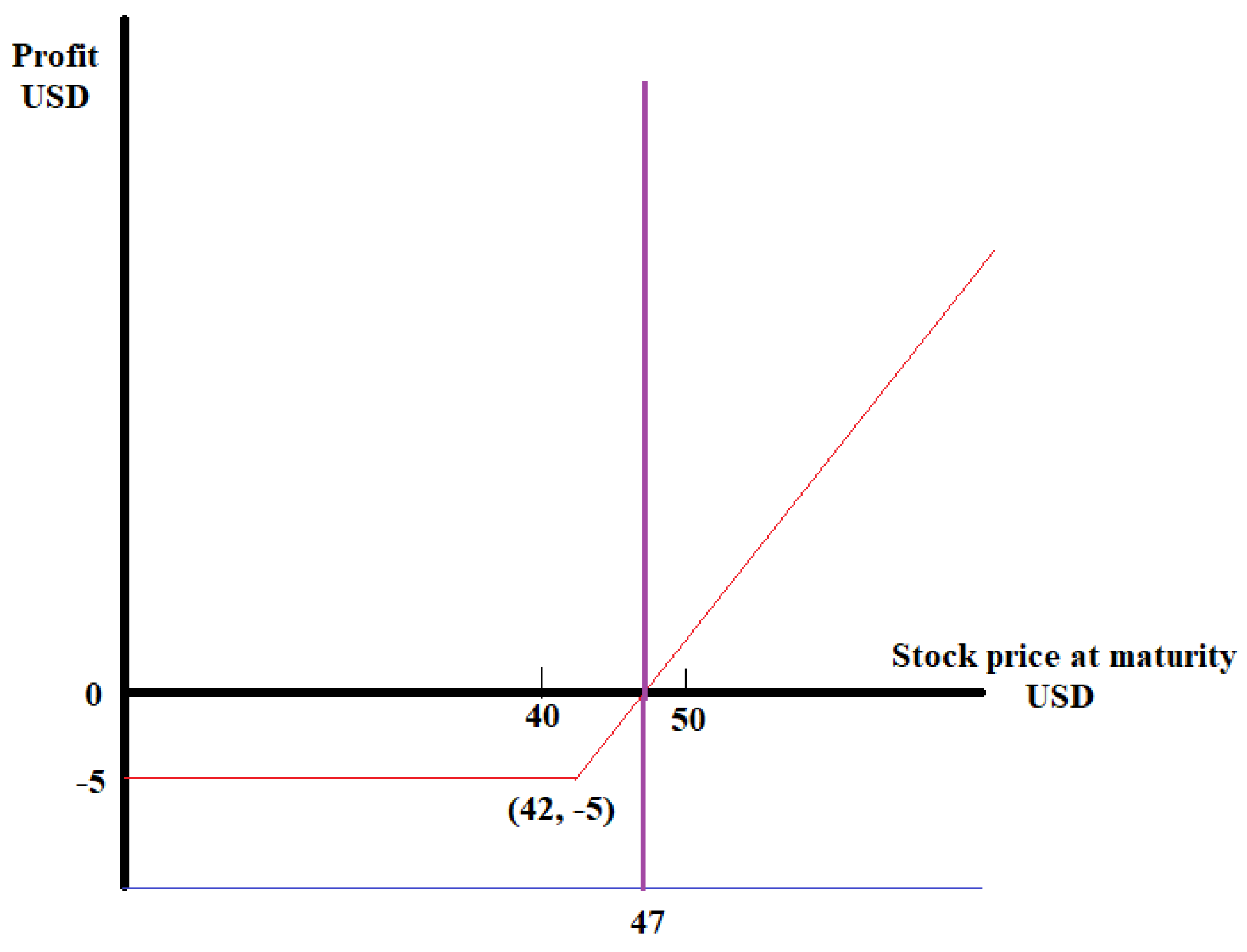
Figure 1. Figure illustrating the pay-offs of the holder of a European call option. Here, the conditions are (1) the option price: USD 5, and (2) the strike price: USD 42. The same example can be found in Reference [2].
Axioms 14 00215 g001
Figure 2. Figure illustrating the pay-offs of the writer of a European call option. Here, the conditions are (1) option price = USD 5, and (2) strike price = USD 42. The same example is analyzed in Reference [2].
Axioms 14 00215 g002
Figure 3. Figure illustrating the pay-offs of the holder of a European put option. The conditions are (1) option price = USD 3 and (2) strike price = USD 50. The same example is analyzed in [2].
Axioms 14 00215 g003
Figure 4. Figure illustrating the pay-offs of the writer of a European put option. The conditions are (1) option price = USD 3 and (2) strike price = USD 50. The same example is analyzed in [2].
Axioms 14 00215 g004
Figure 5. The MG and BS Hamiltonians. The yellow plot corresponds to the MG case with non-trivial volatility, while the blue curve is the BS equation, considering volatility as a parameter (constant for the purpose of the figure).
Axioms 14 00215 g005
Figure 6. The BS Hamiltonian with volatility as a free parameter. The blue plot corresponds to the case with 1 2 σ 2 < r , while the yellow plot corresponds to the case with 1 2 σ 2 > r .
Axioms 14 00215 g006
Figure 7. The sphere is globally inequivalent to a plane. Still, locally, in the neighborhood of a point (the red point in the figure, for example), the sphere is locally equivalent to a plane.
Axioms 14 00215 g007
Disclaimer/Publisher’s Note: The statements, opinions and data contained in all publications are solely those of the individual author(s) and contributor(s) and not of MDPI and/or the editor(s). MDPI and/or the editor(s) disclaim responsibility for any injury to people or property resulting from any ideas, methods, instructions or products referred to in the content.