


An Approach to Generating Fuzzy Rules for a Fuzzy Controller Based on the Decision Tree Interpretation


Abstract
1. Introduction
- The complexity of the control object;
- The complexity of the control task;
- The volume of data available for analysis;
- The time constraints;
- The urgency of the decisions.
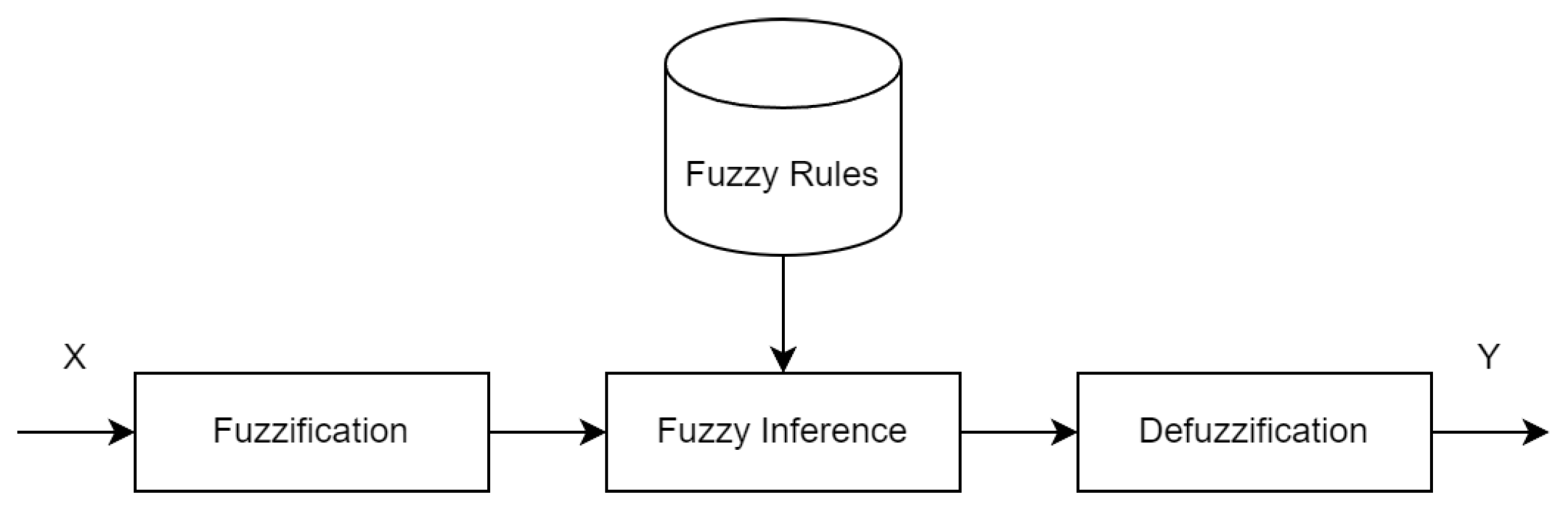
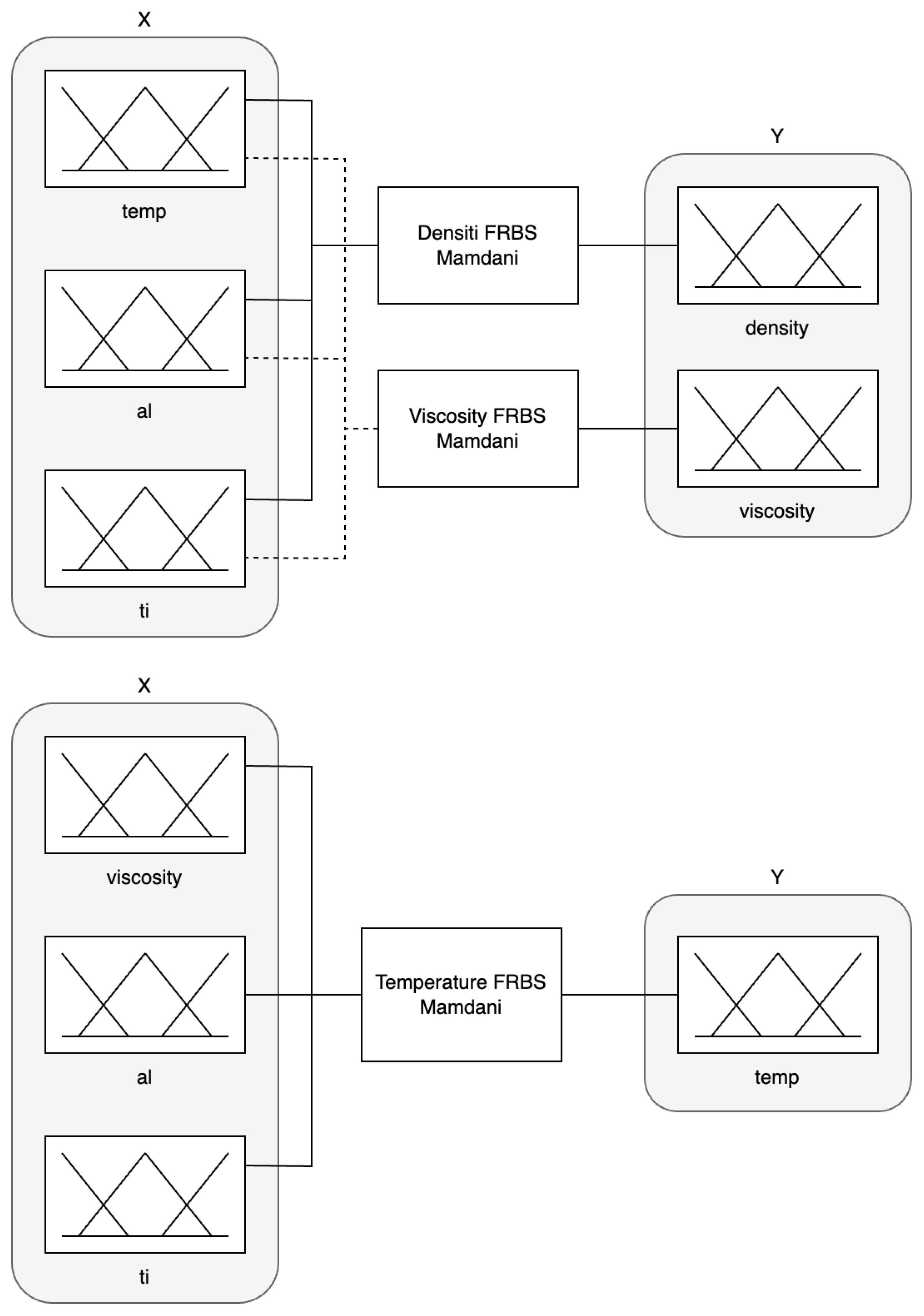
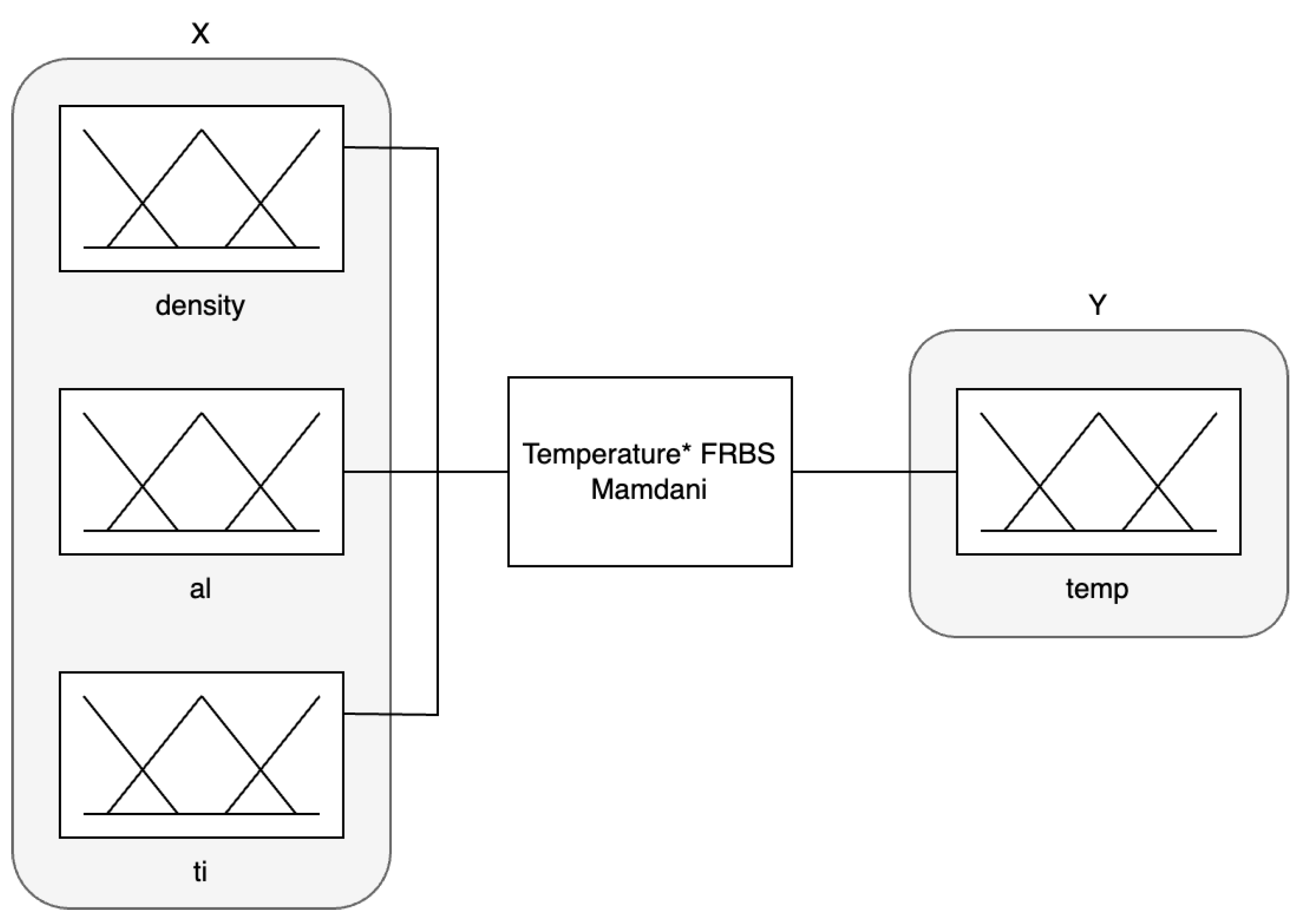
- Fuzzy rule-based systems (FRBSs): FRBSs represent a traditional implementation of an FIS [6]. The structure of an FRBS is illustrated in Figure 1. A collection of numerical (crisp) inputs, denoted as X, is used as the FRBS’s input. This is followed by a fuzzification process, which calculates the membership degree for each input parameter from X in relation to the fuzzy set. Subsequently, fuzzy inference is organized based on a set of fuzzy rules, which determine the knowledge base of the FRBS, describing the behavioral characteristics of an object and its external environment. The defuzzification process then converts the fuzzy inference results into a set of crisp output parameters, represented as Y.
- Genetic/evolutionary fuzzy systems (GFSs): A GFS operates on principles similar to those of an FRBS but uses genetic and evolutionary algorithms to train and fine-tune the parameters [4,7,8]. These evolutionary techniques allow for the optimal set of fuzzy rules to be generated and the membership function parameters to be optimized.
- Neuro fuzzy systems (NFSs): An NFS builds on the FRBS scheme by integrating an FRBS with artificial neural networks. Although the FRBS can interpret the results, neural networks can learn to solve specific tasks [14,15,16]. Neural networks in NFSs are an alternative to the traditional set of fuzzy rules in FRBSs.
- Fuzzification of the input values: Each value of the input variable linked to a fuzzy set A is characterized by a membership degree .
- Aggregation: The truth degree of the antecedent of the i-th rule is calculated based on the aggregation of the membership degrees of the input variables X. The specific aggregation method is determined by the algorithm in use, such as Mamdani, Sugeno, or Tsukamoto.
- Activation: The truth degree of the consequent of the i-th rule is calculated at the activation stage. If the consequent comprises a single fuzzy statement, its truth degree equals the algebraic product of the weight coefficient and the truth degree of an antecedent of the rule. Where the consequent comprises multiple statements, the truth degree of each statement is derived from the algebraic product of the weight coefficient and the truth degree of an antecedent of the rule. If the weight coefficient is unspecified, then the default value is one.
- Accumulation: A membership function F is constructed for all output variables during the accumulation phase. This function is constructed using the max union of the membership degrees of all fuzzy sets related to the k-th output variable .
- Defuzzification: A crisp value for the output variable is derived from the membership function F at the defuzzification stage. Commonly, the center of gravity method is employed for this process.
- The evolving nature of algorithms: An FIS must be capable of adapting to variations in the input data to consider changes in the external environment and the object itself. One potential solution to this problem is the application of fuzzy clustering algorithms [9].
2. Related Works
2.1. Fuzzy Systems in Control
2.2. Evolving Fuzzy Systems
- Updating the system parameters;
- Evolving the structure.
2.3. Fuzzy Logic Types
- Type-1 fuzzy logic;
- Type-2 fuzzy logic;
- Interval type-2 fuzzy logic, etc.
2.4. Fuzzy Rule Generation
3. Materials and Methods
3.1. Schema of the Proposed Approach
- The dataset represents stable physical processes that remain unaffected by external variables;
- The dataset is initially high-quality, eliminating the need for additional time spent on data preparation;
- The dataset is compact and contains a limited number of features, which streamlines the development and debugging of the fuzzy rule generation algorithm.
- There is no requirement to compute or choose various parameters to run the algorithm.
- There is no need to pre-select the features for analysis. The features are automatically chosen during model training based on the Gini index value.
- The algorithm effectively works with outliers, creating separate branches in the tree for the data that contain them.
- It provides a rapid training speed for the model.
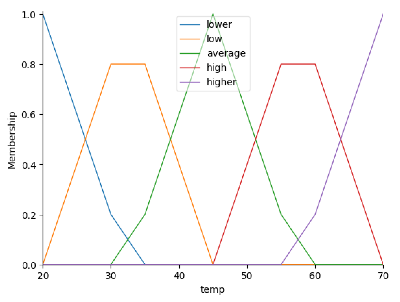
3.2. Description of Fuzzy System
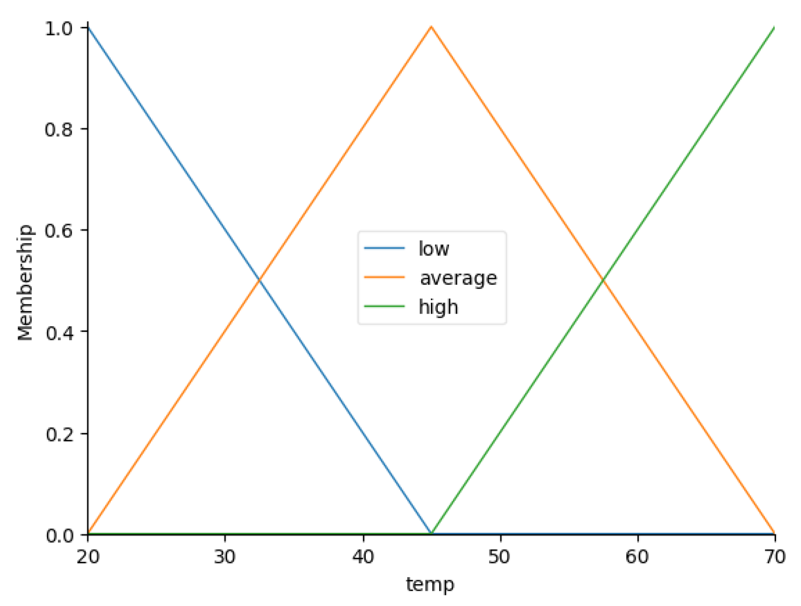
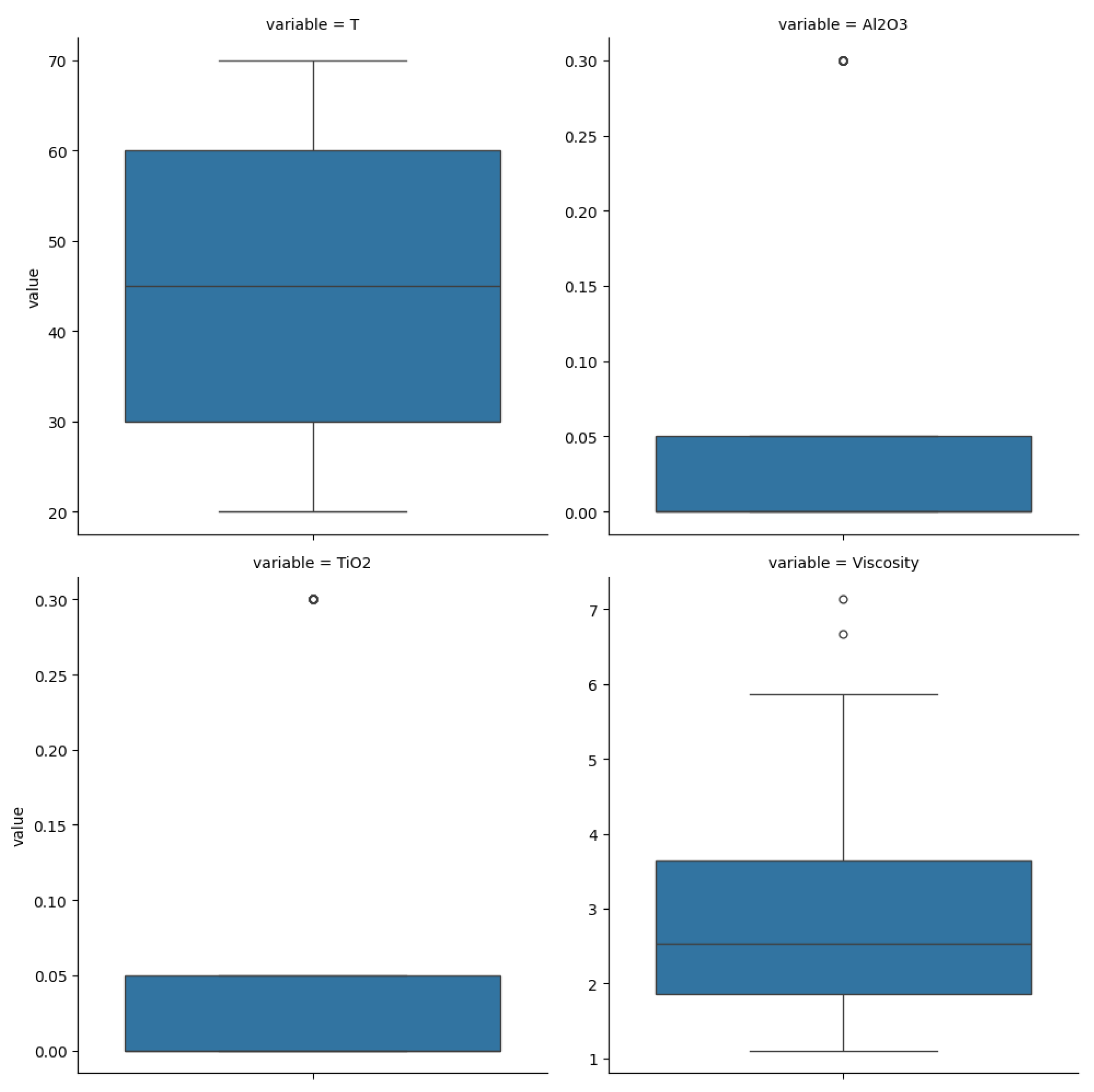
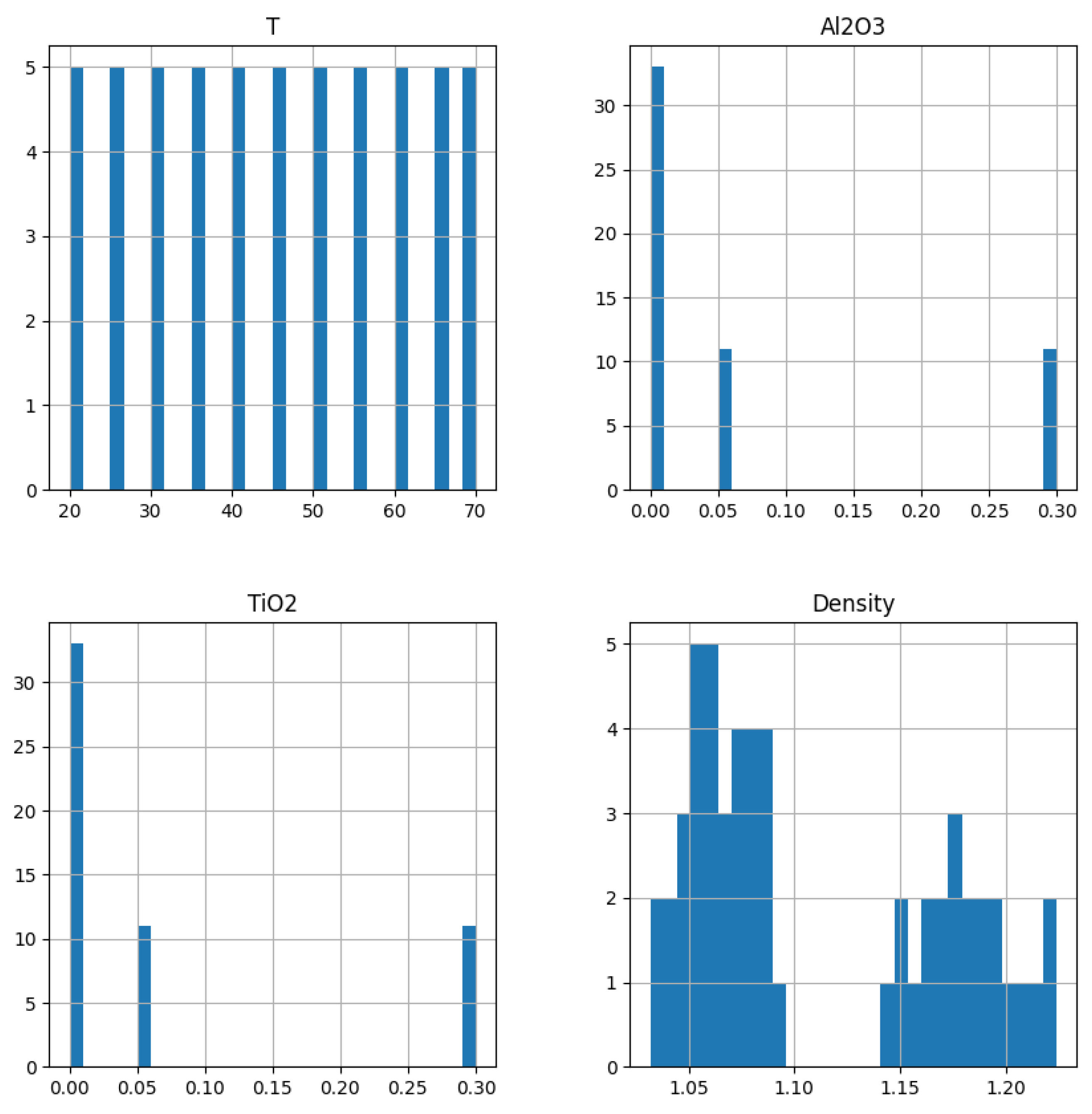
- Temperature (): 20–70 °C;
- Al2O3 concentration (): 0, 0.05, and 0.3 vol %;
- TiO2 concentration (): 0, 0.05, and 0.3 vol %.
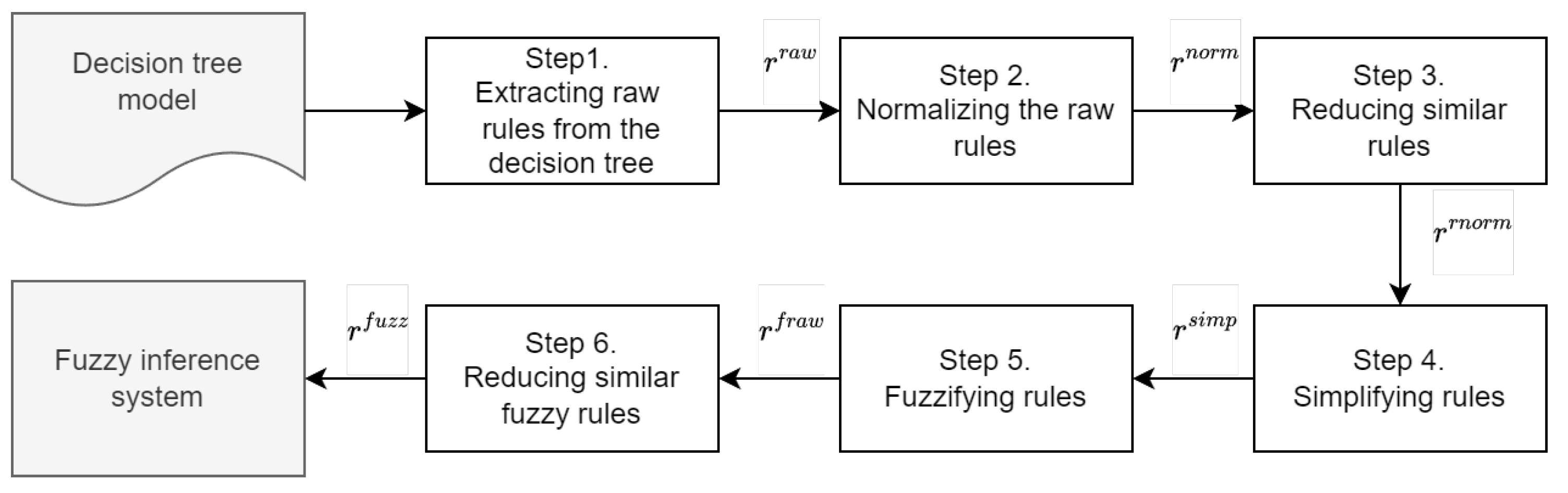
3.3. Description of the Approach to Generating Fuzzy Rules
- Step 1.
- Extracting raw rules from the decision tree. The initial stage involves obtaining a set of raw rules from the decision tree. The set contains crisp rules.
- Step 2.
- Normalizing the raw rules. A set of normalized rules, called , is derived from the raw rules . This step requires eliminating any overlapping statements across all input parameters X to form a normalized rule from the raw rule . The set contains crisp rules.
- Step 3.
- Reducing similar rules. Some normalized rules in may have identical antecedents but different consequents. These rules are classified as similar and should be reduced into a single rule, forming a set of reduced rules denoted as . The set contains crisp rules.
- Step 4.
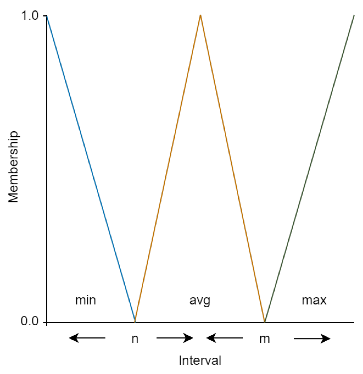
- Simplifying rules. This step involves transitioning from multiple statements in the antecedents of the rules associated with a specific input parameter that use the relations > and ≤ to a single statement with the relation =, which is essential for the construction of fuzzy rules. A set of simplified rules is created from the set of reduced rules . The set consists of crisp rules.
- Step 5.
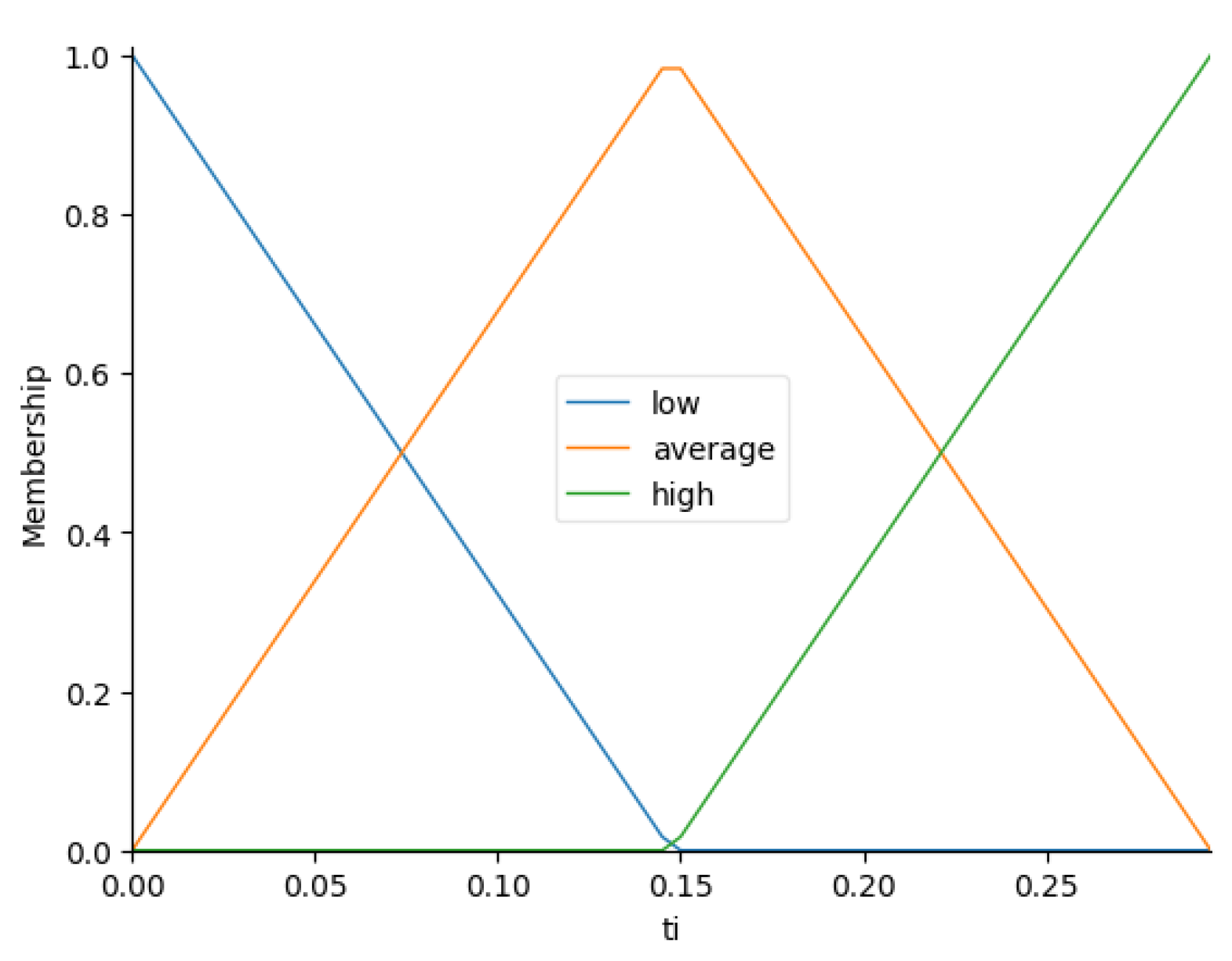
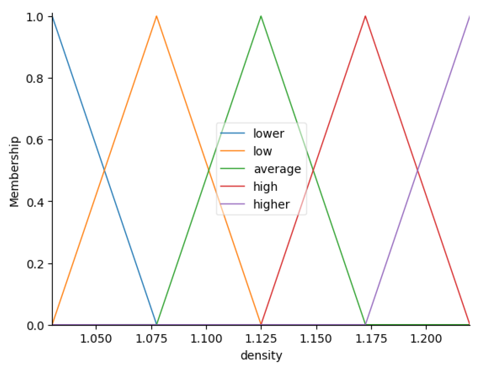
- Fuzzifying rules. It is important to define fuzzy sets for the input parameters X and the output parameters Y to fuzzify the set of rules . This step generates a collection of raw fuzzy rules based on the simplified rules . The set contains fuzzy rules.
- Step 6.
- Reducing similar fuzzy rules. After the previous step, there may be fuzzy rules with similar antecedents but different consequents. In this step, similar fuzzy rules are reduced from the set to arrive at the final collection of fuzzy rules .
3.4. Steps of the Approach to Generating Fuzzy Rules
- Step 1.
- Extracting raw rules from the decision tree
- Step 2.
- Normalization of the raw rules
- Step 3.
- Reducing similar rules
| Algorithm 1 Normalization algorithm |
Input:
Output:
for all
do Create a new normalized rule . for all do Obtain the statements s for an input parameter from the antecedent of the rule . Select from s a statement with and the minimal value : Select from s a statement with and the maximal value : Add statements and to the antecedent of the new rule . end for Add the consequent of the i-th raw rule to the new rule . Add the new rule to the set of normalized rules . end for return
|
| Algorithm 2 Reducing algorithm |
Input:
Output:
Obtain the set of similar rules . Add the rules that are not present in the set to the set . for all
do Select the rules r whose antecedent matches that of the i-th rule from the set of similar rules . Create a new rule by aggregating the rules r and applying the averaging function to the values of the output parameter in the consequent Add the new rule to the set . end for return
|
- Step 4.
- Simplifying rules
| Algorithm 3 Simplifying rule algorithm |
Input:
Output:
for all
do Create a new rule . for all do Obtain the statements s from the antecedent of the rule that describe the left n and right m boundaries of the input parameter : Calculate a new value for a single statement: Create a new statement and add them to the antecedent of the new rule . end for Add the new rule to the set of simplified rules . end for return
|
- Step 5.
- Fuzzifying rules
- Step 6.
- Reducing similar fuzzy rules
| Algorithm 4 Fuzzifying rule algorithm |
Input:
Output:
for all
do Create a new rule . Obtain the statements s from the antecedent of the i-th rule . for all do Fuzzify the value of the j-th statement and select the fuzzy value with the maximal membership degree: Create a new statement and add it to the antecedent of the new rule . end for Fuzzyfy the value of the consequent and select the fuzzy value with maximal membership degree: Add a statement as a consequent of the new rule . Add the new rule to the set of raw fuzzy rules . end for return
|
| Algorithm 5 Reducing similar fuzzy rule algorithm |
Input:
Output:
Obtain the set of similar rules . Add the rules that are not present in the set to the set . for all
do Obtain the rules r whose antecedent matches that of the i-th rule from the set of similar rules . Select the rule from the set of rules r for which the sum of the membership degrees of the statements in the rule antecedent is minimal: Add the rule to the set . end for return |
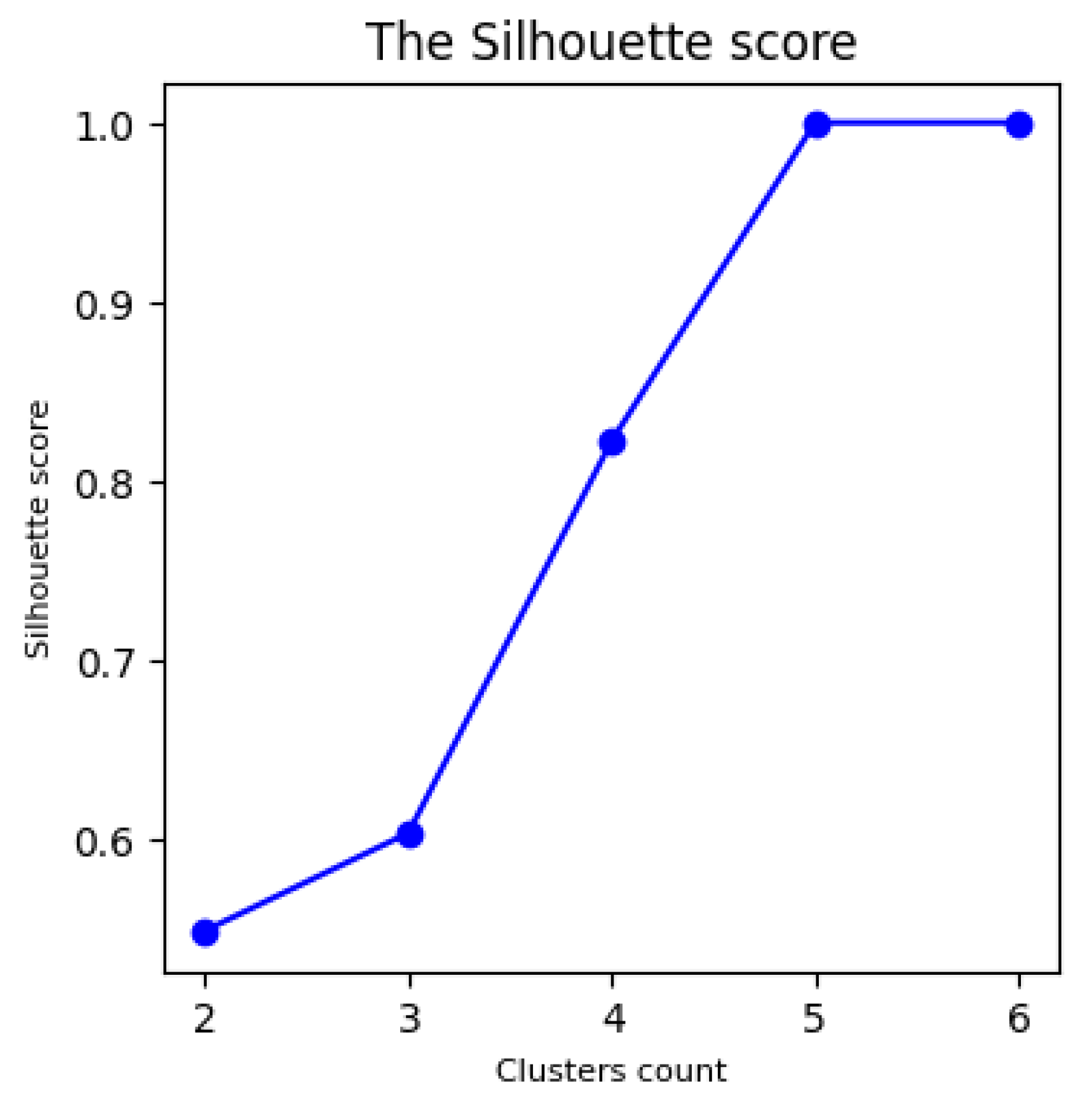
3.5. Rule Clustering
4. Experiments
- Programming language: Python.
- Python interpreter version: 3.12.
- Libraries:
- Machine learning library (including the CART decision trees and KMeans clustering): scikit-learn 1.5.2;
- Data manipulation libraries: numpy 2.1.0 and pandas 2.2.2;
- Fuzzy inference library: scikit-fuzzy 0.5.0;
- Plotting library: matplotlib 3.9.2;
- Additional dependency for the scikit-fuzzy library: networkx 3.4.2.
4.1. Hypothesis 1 Validation
- ;
- ;
- .
- ;
- ;
- .
- ;
- ;
- .
- ;
- ;
- .
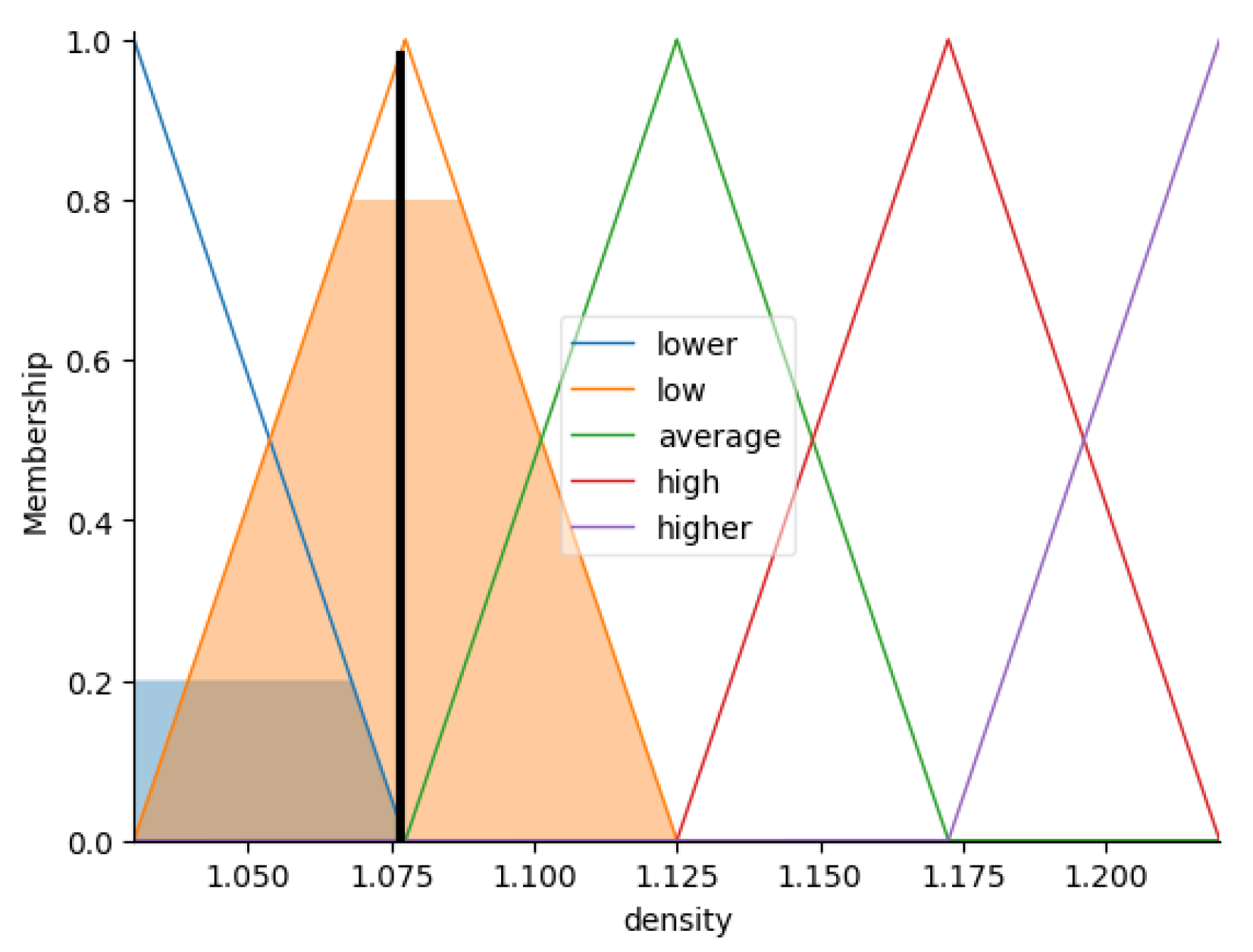
- Fuzzification:
- , , ;
- , , ;
- , , .
- Aggregation and activation:
- For rule;
- For rule;
- For rule, etc.
- Accumulation. Figure 15 represents the accumulation result.
- Defuzzification. and .
- ;
- ;
- .
- ;
- ;
- .
4.2. Hypothesis 2 Validation
- ;
- ;
- .
- ;
- ;
- .
- ;
- ;
- .
4.3. Hypothesis 3 Validation
5. Discussion
- This approach applies to a range of tasks because it is not limited to a specific domain or task;
- This article explains the fuzzy rule generation algorithm, complete with details and examples;
- This article includes experiments that show how the parameters and data quality affect the quality of the resulting FRBS.
6. Conclusions
- The proposed approach facilitates the rapid construction of an FRBS without requiring a profound understanding of the task, its domain, or the analyzed object.
- The performance of the resulting system will be approximately equivalent to that of the decision tree. The performance depends on the proper selection of the optimal number of fuzzy variables and the types and configurations of membership functions. It is important to note that this article does not discuss the selection of the optimal FRBS parameters.
- In certain situations, it may be necessary to modify the generated fuzzy rules. To address this issue, a clustering algorithm has been proposed which can identify groups of similar rules. This approach can help evaluate the extent of the coverage within the solution space.
- The development of an approach to generating a set of fuzzy rules based on the interpretation of other machine learning algorithms;
- The development of a method for generating fuzzy sets considering the specifics of the subject area and data to improve the quality of the FRBS;
- Adapting the proposed approach to be compatible with additional fuzzy inference algorithms.
Author Contributions
Funding
Institutional Review Board Statement
Informed Consent Statement
Data Availability Statement
Conflicts of Interest
Appendix A. The Density Dataset

| # | (°C) | (%) | (%) | |
|---|---|---|---|---|
| training dataset | ||||
| 1 | 20 | 0 | 0 | 1.0625 |
| 2 | 25 | 0 | 0 | 1.05979 |
| 3 | 35 | 0 | 0 | 1.05404 |
| 4 | 40 | 0 | 0 | 1.05103 |
| 5 | 45 | 0 | 0 | 1.04794 |
| 6 | 50 | 0 | 0 | 1.04477 |
| 7 | 60 | 0 | 0 | 1.03826 |
| 8 | 65 | 0 | 0 | 1.03484 |
| 9 | 70 | 0 | 0 | 1.03182 |
| 10 | 20 | 0.05 | 0 | 1.08755 |
| 11 | 45 | 0.05 | 0 | 1.07105 |
| 12 | 50 | 0.05 | 0 | 1.0676 |
| 13 | 55 | 0.05 | 0 | 1.06409 |
| 14 | 65 | 0.05 | 0 | 1.05691 |
| 15 | 70 | 0.05 | 0 | 1.05291 |
| 16 | 20 | 0.3 | 0 | 1.18861 |
| 17 | 25 | 0.3 | 0 | 1.18389 |
| 18 | 30 | 0.3 | 0 | 1.1792 |
| 19 | 40 | 0.3 | 0 | 1.17017 |
| 20 | 45 | 0.3 | 0 | 1.16572 |
| 21 | 50 | 0.3 | 0 | 1.16138 |
| 22 | 55 | 0.3 | 0 | 1.15668 |
| 23 | 60 | 0.3 | 0 | 1.15233 |
| 24 | 70 | 0.3 | 0 | 1.14414 |
| 25 | 20 | 0 | 0.05 | 1.09098 |
| 26 | 25 | 0 | 0.05 | 1.08775 |
| 27 | 30 | 0 | 0.05 | 1.08443 |
| 28 | 35 | 0 | 0.05 | 1.08108 |
| 29 | 40 | 0 | 0.05 | 1.07768 |
| 30 | 60 | 0 | 0.05 | 1.06362 |
| 31 | 65 | 0 | 0.05 | 1.05999 |
| 32 | 70 | 0 | 0.05 | 1.05601 |
| 33 | 25 | 0 | 0.3 | 1.2186 |
| 34 | 35 | 0 | 0.3 | 1.20776 |
| 35 | 45 | 0 | 0.3 | 1.19759 |
| 36 | 50 | 0 | 0.3 | 1.19268 |
| 37 | 55 | 0 | 0.3 | 1.18746 |
| 38 | 65 | 0 | 0.3 | 1.178 |
| testing dataset | ||||
| 1 | 30 | 0 | 0 | 1.05696 |
| 2 | 55 | 0 | 0 | 1.04158 |
| 3 | 25 | 0.05 | 0 | 1.08438 |
| 4 | 30 | 0.05 | 0 | 1.08112 |
| 5 | 35 | 0.05 | 0 | 1.07781 |
| 6 | 40 | 0.05 | 0 | 1.07446 |
| 7 | 60 | 0.05 | 0 | 1.06053 |
| 8 | 35 | 0.3 | 0 | 1.17459 |
| 9 | 65 | 0.3 | 0 | 1.14812 |
| 10 | 45 | 0 | 0.05 | 1.07424 |
| 11 | 50 | 0 | 0.05 | 1.07075 |
| testing dataset | ||||
| 12 | 55 | 0 | 0.05 | 1.06721 |
| 13 | 20 | 0 | 0.3 | 1.22417 |
| 14 | 30 | 0 | 0.3 | 1.2131 |
| 15 | 40 | 0 | 0.3 | 1.20265 |
| 16 | 60 | 0 | 0.3 | 1.18265 |
| 17 | 70 | 0 | 0.3 | 1.17261 |
Appendix B. The Viscosity Dataset
| # | (°C) | (%) | (%) | |
|---|---|---|---|---|
| training dataset | ||||
| 1 | 20 | 0 | 0 | 3.707 |
| 2 | 25 | 0 | 0 | 3.18 |
| 3 | 35 | 0 | 0 | 2.361 |
| 4 | 45 | 0 | 0 | 1.832 |
| 5 | 50 | 0 | 0 | 1.629 |
| 6 | 55 | 0 | 0 | 1.465 |
| 7 | 70 | 0 | 0 | 1.194 |
| 8 | 20 | 0.05 | 0 | 4.66 |
| 9 | 30 | 0.05 | 0 | 3.38 |
| 10 | 35 | 0.05 | 0 | 2.874 |
| 11 | 40 | 0.05 | 0 | 2.489 |
| 12 | 50 | 0.05 | 0 | 1.897 |
| 13 | 55 | 0.05 | 0 | 1.709 |
| 14 | 60 | 0.05 | 0 | 1.47 |
| 15 | 20 | 0.3 | 0 | 6.67 |
| 16 | 25 | 0.3 | 0 | 5.594 |
| 17 | 30 | 0.3 | 0 | 4.731 |
| 18 | 35 | 0.3 | 0 | 4.118 |
| 19 | 40 | 0.3 | 0 | 3.565 |
| 20 | 55 | 0.3 | 0 | 2.426 |
| 21 | 60 | 0.3 | 0 | 2.16 |
| 22 | 70 | 0.3 | 0 | 1.728 |
| 23 | 20 | 0 | 0.05 | 4.885 |
| 24 | 25 | 0 | 0.05 | 4.236 |
| 25 | 35 | 0 | 0.05 | 3.121 |
| 26 | 40 | 0 | 0.05 | 2.655 |
| 27 | 45 | 0 | 0.05 | 2.402 |
| 28 | 50 | 0 | 0.05 | 2.109 |
| 29 | 60 | 0 | 0.05 | 1.662 |
| 30 | 70 | 0 | 0.05 | 1.289 |
| 31 | 20 | 0 | 0.3 | 7.132 |
| 32 | 25 | 0 | 0.3 | 5.865 |
| 33 | 30 | 0 | 0.3 | 4.944 |
| 34 | 35 | 0 | 0.3 | 4.354 |
| 35 | 45 | 0 | 0.3 | 3.561 |
| 36 | 55 | 0 | 0.3 | 2.838 |
| 37 | 60 | 0 | 0.3 | 2.538 |
| 38 | 70 | 0 | 0.3 | 1.9097 |
| testing dataset | ||||
| 1 | 30 | 0 | 0 | 2.716 |
| 2 | 40 | 0 | 0 | 2.073 |
| 3 | 60 | 0 | 0 | 1.329 |
| 4 | 65 | 0 | 0 | 1.211 |
| 5 | 25 | 0.05 | 0 | 4.12 |
| 6 | 45 | 0.05 | 0 | 2.217 |
| 7 | 65 | 0.05 | 0 | 1.315 |
| 8 | 70 | 0.05 | 0 | 1.105 |
| 9 | 45 | 0.3 | 0 | 3.111 |
| 10 | 50 | 0.3 | 0 | 2.735 |
| 11 | 65 | 0.3 | 0 | 1.936 |
| 12 | 30 | 0 | 0.05 | 3.587 |
| 13 | 55 | 0 | 0.05 | 1.953 |
| 14 | 65 | 0 | 0.05 | 1.443 |
| 15 | 40 | 0 | 0.3 | 3.99 |
| 16 | 50 | 0 | 0.3 | 3.189 |
| 17 | 65 | 0 | 0.3 | 2.287 |
Appendix C. The Set of Raw rraw
Appendix D. The Set of Normalized Rules r norm
Appendix E. The Set of Normalized Rules rnorm After Reduction
Appendix F. The Set of Simplified Rules rsimp
Appendix G. The Set of Fuzzy Rules rfuzz
Appendix H. Result of the Rule Clustering
References
- Romanov, A.A.; Filippov, A.A.; Yarushkina, N.G. Adaptive Fuzzy Predictive Approach in Control. Mathematics 2023, 11, 875. [Google Scholar] [CrossRef]
- Romanov, A.; Filippov, A. Context Modeling in Predictive Analytics. In Proceedings of the 2021 International Conference on Information Technology and Nanotechnology (ITNT), Samara, Russia, 20–24 September 2021. [Google Scholar]
- Xu, J.; Wang, Q.; Lin, Q. Parallel Robot with Fuzzy Neural Network Sliding Mode Control. Adv. Mech. Eng. 2018, 10, 1687814018801261. [Google Scholar] [CrossRef]
- Fernandez, A.; Herrera, F.; Cordon, O.; del Jesus, M.J.; Marcelloni, F. Evolutionary Fuzzy Systems for Explainable Artificial Intelligence: Why, When, What For, and Where to? IEEE Comput. Intell. Mag. 2019, 14, 69–81. [Google Scholar] [CrossRef]
- Moral, A.; Castiello, C.; Magdalena, L.; Mencar, C. Explainable Fuzzy Systems; Springer: Berlin, Germany, 2021. [Google Scholar]
- Varshney, A.K.; Torra, V. Literature Review of the Recent Trends and Applications in Various Fuzzy Rule-Based Systems. Int. J. Fuzzy Syst. 2023, 25, 2163–2186. [Google Scholar] [CrossRef]
- Krömer, P.; Platoš, J. Simultaneous Prediction of Wind Speed and Direction by Evolutionary Fuzzy Rule Forest. Procedia Comput. Sci. 2017, 108, 295–304. [Google Scholar] [CrossRef]
- Su, W.C.; Juang, C.F.; Hsu, C.M. Multiobjective Evolutionary Interpretable Type-2 Fuzzy Systems with Structure and Parameter Learning for Hexapod Robot Control. IEEE Trans. Syst. Man Cybern. Syst. 2022, 52, 3066–3078. [Google Scholar] [CrossRef]
- Kerr-Wilson, J.; Pedrycz, W. Generating a Hierarchical Fuzzy Rule-Based Model. Fuzzy Sets Syst. 2020, 381, 124–139. [Google Scholar] [CrossRef]
- Razak, T.R.; Fauzi, S.S.M.; Gining, R.A.J.; Ismail, M.H.; Maskat, R. Hierarchical Fuzzy Systems: Interpretability and Complexity. Indones. J. Electr. Eng. Inform. 2021, 9, 478–489. [Google Scholar] [CrossRef]
- Zouari, M.; Baklouti, N.; Sanchez-Medina, J.; Kammoun, H.M.; Ayed, M.B.; Alimi, A.M. PSO-Based Adaptive Hierarchical Interval Type-2 Fuzzy Knowledge Representation System (PSO-AHIT2FKRS) for Travel Route Guidance. IEEE Trans. Intell. Transport. Syst. 2022, 23, 804–818. [Google Scholar] [CrossRef]
- Roy, D.K.; Saha, K.K.; Kamruzzaman, M.; Biswas, S.K.; Hossain, M.A. Hierarchical Fuzzy Systems Integrated with Particle Swarm Optimization for Daily Reference Evapotranspiration Prediction: A Novel Approach. Water Resour. Manag. 2021, 35, 5383–5407. [Google Scholar] [CrossRef]
- Wei, X.J.; Zhang, D.Q.; Huang, S.J. A Variable Selection Method for a Hierarchical Interval Type-2 TSK Fuzzy Inference System. Fuzzy Sets Syst. 2022, 438, 46–61. [Google Scholar] [CrossRef]
- Karaboga, D.; Kaya, E. Adaptive Network Based Fuzzy Inference System (ANFIS) Training Approaches: A Comprehensive Survey. Artif. Intell. Rev. 2019, 52, 2263–2293. [Google Scholar] [CrossRef]
- Shaik, R.B.; Kannappan, E.V. Application of Adaptive Neuro-Fuzzy Inference Rule-Based Controller in Hybrid Electric Vehicles. J. Electr. Eng. Technol. 2020, 15, 1937–1945. [Google Scholar] [CrossRef]
- Lin, C.-M.; Le, T.-L.; Huynh, T.-T. Self-Evolving Function-Link Interval Type-2 Fuzzy Neural Network for Nonlinear System Identification and Control. Neurocomputing 2018, 275, 2239–2250. [Google Scholar] [CrossRef]
- Li, F.; Yu, F.; Shen, L.; Li, H.; Yang, X.; Shen, Q. EEG-Based emotion recognition with combined fuzzy inference via integrating weighted fuzzy rule inference and interpolation. Mathematics 2025, 13, 166. [Google Scholar] [CrossRef]
- Zadeh, L.A. The Concept of a Linguistic Variable and Its Application to Approximate Reasoning—I. Inf. Sci. 1975, 8, 199–249. [Google Scholar] [CrossRef]
- Zadeh, L.A. Fuzzy Logic. Computer 1988, 21, 83–93. [Google Scholar] [CrossRef]
- Chen, S.; Tsai, F. A New Method to Construct Membership Functions and Generate Fuzzy Rules from Training Instances. Int. J. Inf. Manag. Sci. 2005, 16, 47. [Google Scholar] [CrossRef]
- Wu, T.-P.; Chen, S.-M. A New Method for Constructing Membership Functions and Fuzzy Rules from Training Examples. IEEE Trans. Syst. Man Cybern. B 1999, 29, 25–40. [Google Scholar]
- Jiao, L.; Yang, H.; Liu, Z.G.; Pan, Q. Interpretable Fuzzy Clustering Using Unsupervised Fuzzy Decision Trees. Inf. Sci. 2022, 611, 540–563. [Google Scholar] [CrossRef]
- Idris, N.F.; Ismail, M.A. Breast Cancer Disease Classification Using Fuzzy-ID3 Algorithm with FUZZYDBD Method: Automatic Fuzzy Database Definition. PeerJ Comput. Sci. 2021, 7, e427. [Google Scholar] [CrossRef] [PubMed]
- Al-Gunaid, M.; Shcherbakov, M.; Kamaev, V.; Gerget, O.; Tyukov, A. Decision Trees Based Fuzzy Rules. In Information Technologies in Science, Management, Social Sphere and Medicine; Atlantis Press: Amsterdam, The Netherlands, 2016. [Google Scholar]
- Nagaraj, P.; Deepalakshmi, P. An Intelligent Fuzzy Inference Rule-Based Expert Recommendation System for Predictive Diabetes Diagnosis. Int. J. Imaging Syst. Technol. 2022, 32, 1373–1396. [Google Scholar] [CrossRef]
- Exarchos, T.P.; Tsipouras, M.G.; Exarchos, C.P.; Papaloukas, C.; Fotiadis, D.I.; Michalis, L.K. A Methodology for the Automated Creation of Fuzzy Expert Systems for Ischaemic and Arrhythmic Beat Classification Based on a Set of Rules Obtained by a Decision Tree. Artif. Intell. Med. 2007, 40, 187–200. [Google Scholar] [CrossRef]
- Gu, X.; Han, J.; Shen, Q.; Angelov, P.P. Autonomous learning for fuzzy systems: A review. Artif. Intell. Rev. 2023, 56, 7549–7595. [Google Scholar] [CrossRef]
- Alghamdi, M.; Angelov, P.; Gimenez, R.; Rufino, M.; Soares, E. Self-organising and self-learning model for soybean yield prediction. In Proceedings of the 2019 Sixth International Conference on Social Networks Analysis, Management and Security (SNAMS), Granada, Spain, 22–25 October 2019; pp. 441–446. [Google Scholar]
- Mohamed, S.; Hameed, I.A. A GA-based adaptive neuro-fuzzy controller for greenhouse climate control system. Alex. Eng. J. 2018, 57, 773–779. [Google Scholar] [CrossRef]
- Soares, E.; Angelov, P.; Costa, B.; Castro, M. Actively semi-supervised deep rule-based classifier applied to adverse driving scenarios. In Proceedings of the 2019 International Joint Conference on Neural Networks (IJCNN), Budapest, Hungary, 14–19 July 2019; pp. 1–8. [Google Scholar]
- Andonovski, G.; Sipele, O.; Iglesias, J.A.; Sanchis, A.; Lughofer, E.; Škrjanc, I. Detection of driver maneuvers using evolving fuzzy cloud-based system. In Proceedings of the 2020 IEEE Symposium Series on Computational Intelligence (SSCI), Canberra, Australia, 1–4 December 2020; pp. 700–706. [Google Scholar]
- Wu, Q.; Cheng, S.; Li, L.; Yang, F.; Meng, L.J.; Fan, Z.X.; Liang, H.W. A fuzzy-inference-based reinforcement learning method of overtaking decision making for automated vehicles. Proc. Inst. Mech. Eng. Part D J. Automob. Eng. 2022, 236, 75–83. [Google Scholar] [CrossRef]
- Stirling, J.; Chen, T.; Bucholc, M. Diagnosing Alzheimer’s disease using a self-organising fuzzy classifier. In Fuzzy Logic: Recent Applications and Developments; Springer International Publishing: Cham, Switzerland, 2021; pp. 69–82. [Google Scholar]
- de Campos Souza, P.V.; Lughofer, E. Identification of heart sounds with an interpretable evolving fuzzy neural network. Sensors 2020, 20, 6477. [Google Scholar] [CrossRef]
- Kukker, A.; Sharma, R. A genetic algorithm assisted fuzzy Q-learning epileptic seizure classifier. Comput. Electr. Eng. 2021, 92, 107154. [Google Scholar] [CrossRef]
- Severiano, C.A.; e Silva, P.C.D.L.; Cohen, M.W.; Guimarães, F.G. Evolving fuzzy time series for spatio-temporal forecasting in renewable energy systems. Renew. Energy 2021, 171, 764–783. [Google Scholar] [CrossRef]
- Andonovski, G.; Lughofer, E.; Škrjanc, I. Evolving fuzzy model identification of nonlinear Wiener-Hammerstein processes. IEEE Access 2021, 9, 158470–158480. [Google Scholar] [CrossRef]
- Blažič, A.; Škrjanc, I.; Logar, V. Soft sensor of bath temperature in an electric arc furnace based on a data-driven Takagi–Sugeno fuzzy model. Appl. Soft Comput. 2021, 113, 107949. [Google Scholar] [CrossRef]
- Alfaverh, F.; Denai, M.; Sun, Y. Demand response strategy based on reinforcement learning and fuzzy reasoning for home energy management. IEEE Access 2020, 8, 39310–39321. [Google Scholar] [CrossRef]
- Pratama, M.; Dimla, E.; Tjahjowidodo, T.; Pedrycz, W.; Lughofer, E. Online tool condition monitoring based on parsimonious ensemble+. IEEE Trans. Cybern. 2018, 50, 664–677. [Google Scholar] [CrossRef]
- Camargos, M.O.; Bessa, I.; D’Angelo, M.F.S.V.; Cosme, L.B.; Palhares, R.M. Data-driven prognostics of rolling element bearings using a novel error based evolving Takagi–Sugeno fuzzy model. Appl. Soft Comput. 2020, 96, 106628. [Google Scholar] [CrossRef]
- Malik, H.; Sharma, R.; Mishra, S. Fuzzy reinforcement learning based intelligent classifier for power transformer faults. ISA Trans. 2020, 101, 390–398. [Google Scholar] [CrossRef]
- Rodrigues Júnior, S.E.; de Oliveira Serra, G.L. Intelligent forecasting of time series based on evolving distributed Neuro-Fuzzy network. Comput. Intell. 2020, 36, 1394–1413. [Google Scholar] [CrossRef]
- Cao, B.; Zhao, J.; Lv, Z.; Gu, Y.; Yang, P.; Halgamuge, S.K. Multiobjective evolution of fuzzy rough neural network via distributed parallelism for stock prediction. IEEE Trans. Fuzzy Syst. 2020, 28, 939–952. [Google Scholar] [CrossRef]
- Yarushkina, N.; Filippov, A.; Romanov, A. Contextual Analysis of Financial Time Series. Mathematics 2024, 13, 57. [Google Scholar] [CrossRef]
- Precup, R.E.; Teban, T.A.; Albu, A.; Borlea, A.B.; Zamfirache, I.A.; Petriu, E.M. Evolving fuzzy models for prosthetic hand myoelectric-based control. IEEE Trans. Instrum. Meas. 2020, 69, 4625–4636. [Google Scholar] [CrossRef]
- Yang, Z.X.; Rong, H.J.; Wong, P.K.; Angelov, P.; Yang, Z.X.; Wang, H. Self-evolving data cloud-based PID-like controller for nonlinear uncertain systems. IEEE Trans. Ind. Electron. 2020, 68, 4508–4518. [Google Scholar] [CrossRef]
- Zhang, H.; Zhang, K.; Cai, Y.; Han, J. Adaptive fuzzy fault-tolerant tracking control for partially unknown systems with actuator faults via integral reinforcement learning method. IEEE Trans. Fuzzy Syst. 2019, 27, 1986–1998. [Google Scholar] [CrossRef]
- Gu, X.; Khan, M.A.; Angelov, P.; Tiwary, B.; Yourdshah, E.S.; Yang, Z.X. A novel self-organizing PID approach for controlling mobile robot locomotion. In Proceedings of the 2020 IEEE International Conference on Fuzzy Systems (FUZZ-IEEE), Glasgow, UK, 19–24 July 2020; pp. 1–10. [Google Scholar]
- Juang, C.F.; Lu, C.H.; Huang, C.A. Navigation of three cooperative object-transportation robots using a multistage evolutionary fuzzy control approach. IEEE Trans. Cybern. 2020, 52, 3606–3619. [Google Scholar] [CrossRef] [PubMed]
- Goharimanesh, M.; Mehrkish, A.; Janabi-Sharifi, F. A fuzzy reinforcement learning approach for continuum robot control. J. Intell. Robot. Syst. 2020, 100, 809–826. [Google Scholar] [CrossRef]
- Leite, D.; Škrjanc, I. Ensemble of evolving optimal granular experts, OWA aggregation, and time series prediction. Inf. Sci. 2019, 504, 95–112. [Google Scholar] [CrossRef]
- Azad, A.; Kashi, H.; Farzin, S.; Singh, V.P.; Kisi, O.; Karami, H.; Sanikhani, H. Novel approaches for air temperature prediction: A comparison of four hybrid evolutionary fuzzy models. Meteorol. Appl. 2020, 27, e1817. [Google Scholar] [CrossRef]
- Malik, H.; Yadav, A.K. A novel hybrid approach based on relief algorithm and fuzzy reinforcement learning approach for predicting wind speed. Sustain. Energy Technol. Assess. 2021, 43, 100920. [Google Scholar] [CrossRef]
- Ge, D.; Zeng, X.J. Learning data streams online—An evolving fuzzy system approach with self-learning/adaptive thresholds. Inf. Sci. 2020, 507, 172–184. [Google Scholar] [CrossRef]
- Gu, X.; Shen, Q. A self-adaptive fuzzy learning system for streaming data prediction. Inf. Sci. 2021, 579, 623–647. [Google Scholar] [CrossRef]
- Angelov, P.P.; Filev, D.P. An approach to online identification of Takagi-Sugeno fuzzy models. IEEE Trans. Syst. Man Cybern. Part B (Cybern.) 2004, 34, 484–498. [Google Scholar] [CrossRef]
- Gu, X.; Angelov, P.P. Self-organising fuzzy logic classifier. Inf. Sci. 2018, 447, 36–51. [Google Scholar] [CrossRef]
- Rong, H.J.; Yang, Z.X.; Wong, P.K. Robust and noise-insensitive recursive maximum correntropy-based evolving fuzzy system. IEEE Trans. Fuzzy Syst. 2019, 28, 2277–2284. [Google Scholar] [CrossRef]
- Ferdaus, M.M.; Pratama, M.; Anavatti, S.G.; Garratt, M.A. PALM: An incremental construction of hyperplanes for data stream regression. IEEE Trans. Fuzzy Syst. 2019, 27, 2115–2129. [Google Scholar] [CrossRef]
- Yang, Z.X.; Rong, H.J.; Angelov, P.; Yang, Z.X. Statistically evolving fuzzy inference system for non-Gaussian noises. IEEE Trans. Fuzzy Syst. 2021, 30, 2649–2664. [Google Scholar] [CrossRef]
- Samanta, S.; Pratama, M.; Sundaram, S. A novel spatio-temporal fuzzy inference system (SPATFIS) and its stability analysis. Inf. Sci. 2019, 505, 84–99. [Google Scholar] [CrossRef]
- Pratama, M.; Anavatti, S.G.; Lughofer, E. GENEFIS: Toward an effective localist network. IEEE Trans. Fuzzy Syst. 2013, 22, 547–562. [Google Scholar] [CrossRef]
- Jahanshahi, H.; Yousefpour, A.; Soradi-Zeid, S.; Castillo, O. A review on design and implementation of type-2 fuzzy controllers. Math. Methods Appl. Sci. 2022. [Google Scholar] [CrossRef]
- Mendel, J.; Hagras, H.; Tan, W.W.; Melek, W.W.; Ying, H. Introduction to Type-2 Fuzzy Logic Control: Theory and Applications; John Wiley & Sons: Hoboken, NJ, USA, 2014. [Google Scholar]
- Mirnezami, S.A.; Mousavi, S.M.; Mohagheghi, V. An innovative interval type-2 fuzzy approach for multi-scenario multi-project cash flow evaluation considering TODIM and critical chain with an application to energy sector. Neural Comput. Appl. 2021, 33, 2263–2284. [Google Scholar] [CrossRef]
- Ecer, F. Multi-criteria decision making for green supplier selection using interval type-2 fuzzy AHP: A case study of a home appliance manufacturer. Oper. Res. 2022, 22, 199–233. [Google Scholar] [CrossRef]
- Aleksić, A.; Milanović, D.D.; Komatina, N.; Tadić, D. Evaluation and ranking of failures in manufacturing process by combining best-worst method and VIKOR under type-2 fuzzy environment. Expert Syst. 2023, 40, e13148. [Google Scholar] [CrossRef]
- Said, Z.; Abdelkareem, M.A.; Rezk, H.; Nassef, A.M. Dataset on Fuzzy Logic Based-Modelling and Optimization of Thermophysical Properties of Nanofluid Mixture. Data Brief 2019, 26, 104547. [Google Scholar] [CrossRef]
- Said, Z.; Abdelkareem, M.A.; Rezk, H.; Nassef, A.M. Fuzzy Modeling and Optimization for Experimental Thermophysical Properties of Water and Ethylene Glycol Mixture for Al2O3 and TiO2 Based Nanofluids. Powder Technol. 2019, 353, 345–358. [Google Scholar] [CrossRef]
- James, G.; Witten, D.; Hastie, T.; Tibshirani, R. An Introduction to Statistical Learning; Springer: New York, NY, USA, 2013. [Google Scholar]
- Fuzzy Logic Toolbox. Available online: https://www.mathworks.com/products/fuzzy-logic.html (accessed on 10 January 2025).
- Mamdani, E.H. Application of fuzzy algorithms for control of simple dynamic plant. Proc. Inst. Electr. Eng. 1974, 121, 1585–1588. [Google Scholar] [CrossRef]
- Aggarwal, A. A Beginner’s Guide to Fuzzy Logic Controllers for AC Temperature Control. Available online: https://threws.com/a-beginners-guide-to-fuzzy-logic-controllers-for-ac-temperature-control/ (accessed on 1 November 2024).
- Płoński, P. Extract Rules from Decision Tree in 3 Ways with Scikit-Learn and Python. Available online: https://mljar.com/blog/extract-rules-decision-tree/ (accessed on 1 November 2024).
- Silhouette Coefficient. Available online: https://scikit-learn.org/dev/modules/clustering.html#silhouette-coefficient (accessed on 1 November 2024).
- Kliegr, T.; Bahník, Š.; Fürnkranz, J. A review of possible effects of cognitive biases on interpretation of rule-based machine learning models. Artif. Intell. 2021, 295, 103458. [Google Scholar] [CrossRef]
| Topic | Keywords | Period |
|---|---|---|
| Fuzzy systems in control | “fuzzy systems” in control | From 2019 |
| Trends and challenges in fuzzy system development | “fuzzy rule based systems” recent trends review | |
| Challenges in the explainability of fuzzy systems | ”fuzzy systems” explainability | |
| Representation of knowledge and rules based on fuzzy logic | “fuzzy knowledge representation” “fuzzy rules” | |
| Types of fuzzy logic | type-2 fuzzy systems review | |
| Integration of fuzzy systems and neural networks | anfis “adaptive Neuro fuzzy inference system” | |
| Hierarchical fuzzy systems | hierarchical fuzzy systems | |
| Evolutionary fuzzy systems | evolutionary fuzzy systems | |
| Selection of the optimal parameters for fuzzy systems | “membership functions” construction | |
| Generation of fuzzy rules based on a decision tree | “decision tree” “fuzzy rules” generation |
| # | (°C) Viscosity (Pa·s) | (%) | (%) | Real | Inferred | RMSE |
|---|---|---|---|---|---|---|
| Density FRBS | ||||||
| 1 | 30 | 0 | 0 | 1.056 | 1.073 | 0.017 |
| 2 | 55 | 0 | 0 | 1.041 | 1.047 | 0.006 |
| 3 | 25 | 0.05 | 0 | 1.084 | 1.076 | 0.008 |
| 4 | 30 | 0.05 | 0 | 1.081 | 1.073 | 0.007 |
| 5 | 35 | 0.05 | 0 | 1.077 | 1.069 | 0.009 |
| 6 | 40 | 0.05 | 0 | 1.074 | 1.067 | 0.007 |
| 7 | 60 | 0.05 | 0 | 1.061 | 1.067 | 0.007 |
| 8 | 35 | 0.3 | 0 | 1.174 | 1.172 | 0.002 |
| 9 | 65 | 0.3 | 0 | 1.148 | 1.136 | 0.012 |
| 10 | 45 | 0 | 0.05 | 1.074 | 1.067 | 0.007 |
| 11 | 50 | 0 | 0.05 | 1.071 | 1.067 | 0.004 |
| 12 | 55 | 0 | 0.05 | 1.067 | 1.068 | 0.001 |
| 13 | 20 | 0 | 0.3 | 1.224 | 1.204 | 0.020 |
| 14 | 30 | 0 | 0.3 | 1.213 | 1.202 | 0.011 |
| 15 | 40 | 0 | 0.3 | 1.202 | 1.203 | 0.001 |
| 16 | 60 | 0 | 0.3 | 1.182 | 1.176 | 0.007 |
| 17 | 70 | 0 | 0.3 | 1.172 | 1.172 | 0.000 |
| Total | 0.009 | |||||
| Viscosity FRBS | ||||||
| 1 | 30 | 0 | 0 | 2.716 | 3.089 | 0.374 |
| 2 | 40 | 0 | 0 | 2.073 | 2.359 | 0.287 |
| 3 | 60 | 0 | 0 | 1.329 | 1.465 | 0.137 |
| 4 | 65 | 0 | 0 | 1.211 | 1.414 | 0.204 |
| 5 | 25 | 0.05 | 0 | 4.120 | 3.188 | 0.931 |
| 6 | 45 | 0.05 | 0 | 2.217 | 2.045 | 0.171 |
| 7 | 65 | 0.05 | 0 | 1.315 | 1.414 | 0.100 |
| 8 | 70 | 0.05 | 0 | 1.105 | 1.408 | 0.304 |
| 9 | 45 | 0.3 | 0 | 3.111 | 3.499 | 0.388 |
| 10 | 50 | 0.3 | 0 | 2.735 | 3.475 | 0.740 |
| 11 | 65 | 0.3 | 0 | 1.936 | 1.812 | 0.124 |
| 12 | 30 | 0 | 0.05 | 3.587 | 3.111 | 0.475 |
| 13 | 55 | 0 | 0.05 | 1.953 | 2.128 | 0.176 |
| 14 | 65 | 0 | 0.05 | 1.443 | 1.414 | 0.028 |
| 15 | 40 | 0 | 0.3 | 3.990 | 3.475 | 0.515 |
| 16 | 50 | 0 | 0.3 | 3.189 | 3.475 | 0.286 |
| 17 | 65 | 0 | 0.3 | 2.287 | 1.812 | 0.475 |
| Total | 0.407 | |||||
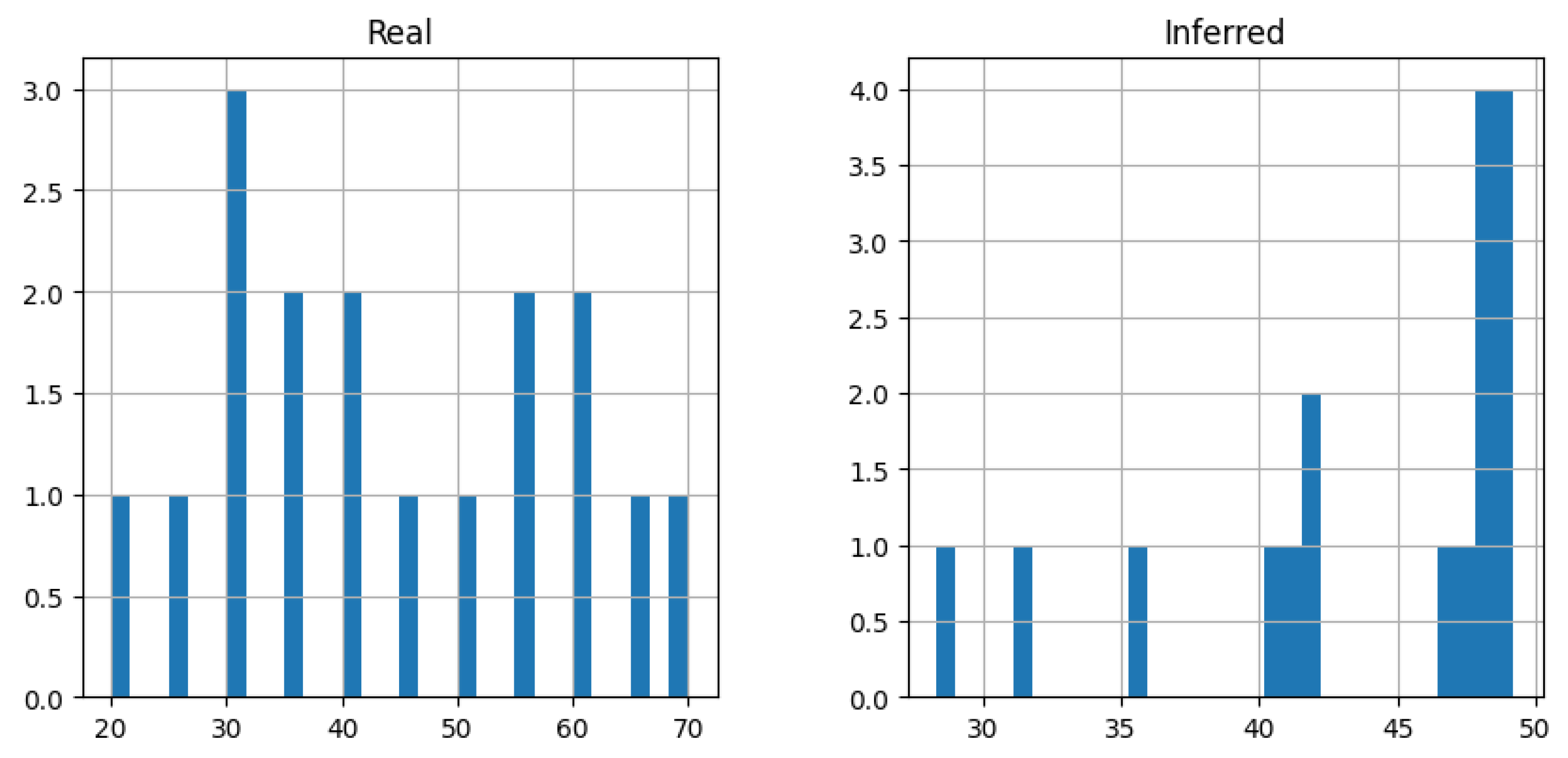
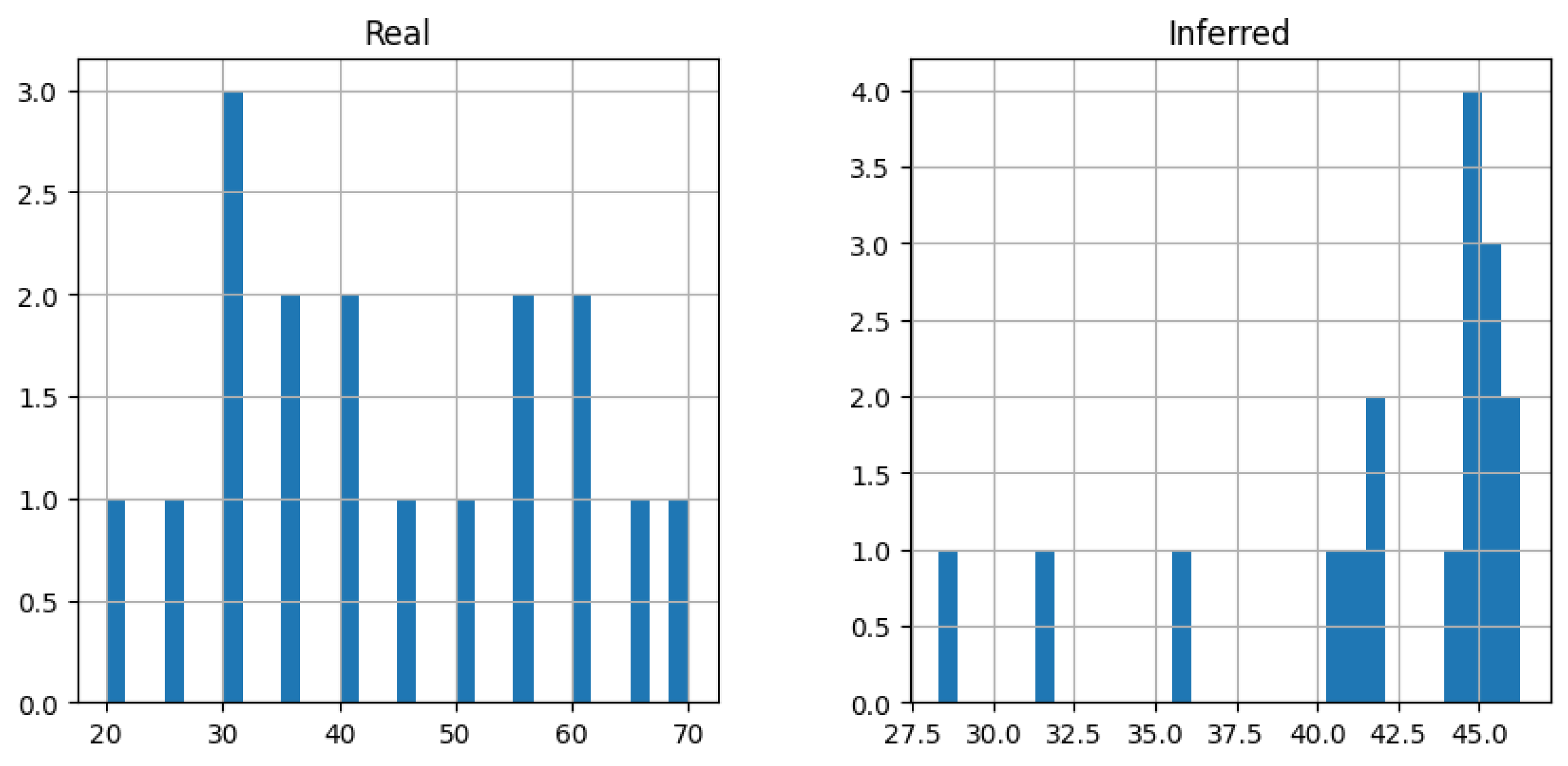
| Temperature FRBS | ||||||
| 1 | 2.716 | 0 | 0 | 30 | 48.540 | 18.540 |
| 2 | 2.073 | 0 | 0 | 40 | 51.739 | 11.739 |
| 3 | 1.329 | 0 | 0 | 60 | 58.696 | 1.304 |
| 4 | 1.211 | 0 | 0 | 65 | 63.509 | 1.491 |
| 5 | 4.120 | 0.05 | 0 | 25 | 30.269 | 5.269 |
| 6 | 2.217 | 0.05 | 0 | 45 | 52.190 | 7.190 |
| Temperature FRBS | ||||||
| 7 | 1.315 | 0.05 | 0 | 65 | 59.122 | 5.878 |
| 8 | 1.105 | 0.05 | 0 | 70 | 65.513 | 4.487 |
| 9 | 3.111 | 0.3 | 0 | 45 | 44.290 | 0.710 |
| 10 | 2.735 | 0.3 | 0 | 50 | 52.520 | 2.520 |
| 11 | 1.936 | 0.3 | 0 | 65 | 59.258 | 5.742 |
| 12 | 3.587 | 0 | 0.05 | 30 | 34.285 | 4.285 |
| 13 | 1.953 | 0 | 0.05 | 55 | 51.675 | 3.325 |
| 14 | 1.443 | 0 | 0.05 | 65 | 56.137 | 8.863 |
| 15 | 3.990 | 0 | 0.3 | 40 | 38.163 | 1.838 |
| 16 | 3.189 | 0 | 0.3 | 50 | 44.909 | 5.092 |
| 17 | 2.287 | 0 | 0.3 | 65 | 59.971 | 5.029 |
| Total | 6.954 | |||||
Disclaimer/Publisher’s Note: The statements, opinions and data contained in all publications are solely those of the individual author(s) and contributor(s) and not of MDPI and/or the editor(s). MDPI and/or the editor(s) disclaim responsibility for any injury to people or property resulting from any ideas, methods, instructions or products referred to in the content. |
© 2025 by the authors. Licensee MDPI, Basel, Switzerland. This article is an open access article distributed under the terms and conditions of the Creative Commons Attribution (CC BY) license (https://creativecommons.org/licenses/by/4.0/).
Share and Cite
Romanov, A.A.; Filippov, A.A.; Yarushkina, N.G. An Approach to Generating Fuzzy Rules for a Fuzzy Controller Based on the Decision Tree Interpretation. Axioms 2025, 14, 196. https://doi.org/10.3390/axioms14030196
Romanov AA, Filippov AA, Yarushkina NG. An Approach to Generating Fuzzy Rules for a Fuzzy Controller Based on the Decision Tree Interpretation. Axioms. 2025; 14(3):196. https://doi.org/10.3390/axioms14030196
Chicago/Turabian StyleRomanov, Anton A., Aleksey A. Filippov, and Nadezhda G. Yarushkina. 2025. "An Approach to Generating Fuzzy Rules for a Fuzzy Controller Based on the Decision Tree Interpretation" Axioms 14, no. 3: 196. https://doi.org/10.3390/axioms14030196
APA StyleRomanov, A. A., Filippov, A. A., & Yarushkina, N. G. (2025). An Approach to Generating Fuzzy Rules for a Fuzzy Controller Based on the Decision Tree Interpretation. Axioms, 14(3), 196. https://doi.org/10.3390/axioms14030196