Study on Discrete Mosquito Population-Control Models with Allee Effect

Abstract

In this study, two discrete mosquito population-control models incorporating the Allee effect are developed to investigate the impact of different sterile mosquito release strategies. By applying the theory of difference equations, a comprehensive analysis is conducted on the existence and stability of fixed points in scenarios with and without sterile mosquito releases. Conditions for the existence and stability of positive fixed points are rigorously derived. The findings reveal that in the absence of a positive fixed point, the wild mosquito population inevitably declines to extinction. When a single positive fixed point exists, the population dynamics exhibit dependence on the initial population size, potentially leading to either extinction or stabilization. In cases where two positive fixed points are present, a bistable dynamic emerges, indicating the coexistence of two mosquito populations.

1. Introduction

The technique of releasing sterile mosquitoes to suppress wild mosquito populations involves sterilizing male mosquitoes through radiation or genetic engineering and subsequently releasing them into the wild to mate with females [1]. Since these sterile male mosquitoes cannot produce viable offspring, this strategy can effectively reduce the overall mosquito population over time [2].

A critical factor in the success of this method is the sexual lifespan of sterile mosquitoes, which refers to the duration during which sterile male mosquitoes remain capable of mating. For optimal results, the survivability and sexual lifespan of sterile male mosquitoes should ideally match those of their wild counterparts to ensure sufficient opportunities for mating with female mosquitoes [3]. On average, male mosquitoes have a relatively short lifespan—typically around one week. Nevertheless, this duration is generally adequate for them to seek out and mate with female mosquitoes in their natural habitat. However, studies have indicated that the sterilization process may negatively affect mosquito longevity. Although the impact can be mitigated through optimized treatment protocols, sterile mosquitoes often exhibit a shorter lifespan and reduced sexual viability compared to their wild counterparts [4].

In this context, Yu et al. introduced a class of time-delayed differential equation models that incorporated the concept of the sexual lifespan of sterile mosquitoes into mathematical modeling [5]. In their work, only sexually active sterile mosquitoes were considered in the interaction dynamics between wild and sterile mosquito populations. Based on this approach, Yu and his collaborators developed several continuous mathematical models and conducted dynamic analyses to examine the effects of different release strategies on the suppression of wild mosquito populations [6,7,8,9,10].

The Allee effect is a biological phenomenon where the per capita growth rate of a population decreases at low population densities. This effect arises due to challenges such as difficulty in finding mates, reduced cooperative behaviors, or inefficient resource utilization. In the context of mosquito populations, the Allee effect is particularly significant because their reproduction and development heavily depend on specific environmental resources, such as breeding sites (e.g., stagnant water bodies like puddles, ponds, or wetlands) and food availability. When these resources are scarce or unevenly distributed, the reproductive efficiency of mosquito populations can be severely impaired [11]. For example, in environments where breeding sites are limited, female mosquitoes may struggle to find suitable locations to lay eggs, and the likelihood of successful mating between males and females may decrease. This resource scarcity leads to a reduction in the per capita growth rate, as fewer offspring are produced. The Allee effect captures this phenomenon by modeling the relationship between population density and reproductive success, highlighting how resource limitations can suppress population growth. Li Jia et al. [12] considered this mating difficulty within populations by the Allee effect and constructed a discrete dynamic system to explore the system’s dynamic properties.

Incorporating the Allee effect into mosquito population models is crucial for accurately predicting population dynamics under varying environmental conditions. It is especially important when evaluating the effectiveness of sterile mosquito release strategies. If the wild mosquito population is already at a low density due to resource scarcity, the Allee effect may further hinder its recovery, potentially enhancing the impact of sterile mosquito releases. By considering the Allee effect, models can better reflect the complex interactions between population density, resource availability, and reproductive success, providing a more robust framework for designing and optimizing mosquito control strategies.

In this work, we will construct discrete dynamic models with Allee effect based on the developmental characteristics of wild mosquito populations and study two different release strategies for sterile mosquitoes. The structure of this paper is as follows: In Section 2, we will develop a model for the development of wild mosquito populations without considering the release of sterile mosquitoes, and analyze the existence and stability of its fixed points. Building on this, Section 3 introduces a constant release of sterile mosquitoes and investigates the system’s dynamic behavior, determining the release threshold that ensures the extinction of the wild mosquito population. Section 4 considers the proportional release of sterile mosquitoes, discussing the types of fixed points and the release-rate threshold. Finally, Section 5 provides a brief conclusion.

2. Wild Mosquito Population Development Model

To facilitate the description of sterile mosquito release timings, we establish the difference equations with a more generalized or arbitrary iteration interval, rather than using generations as the unit of time. This is based on the corresponding biological growth conditions and the release cycle of sterile mosquitoes.

When the growth stage and sex of individuals are not distinguished, we can assume that the mosquito population is homogeneous. In this case, let $M_n$ represent the size of the wild mosquito population at time point n. Referring to the approach in the literature [13], the cyclical development of the wild mosquito population in the absence of sterile mosquito release can be described by the following equation:

$$M_{n+1}=A\left(M_n\right)M_{n}S\left(M_n\right)+\mu M_n,$$

(1)

where $A\left(M_n\right)$ represents the birth-rate function, $S\left(M_n\right)$ denotes the probability that offspring survive to the next time point $n+1$, and $0<\mu <1$ represents the survival rate of adult wild mosquitoes. It is important to note that although the population is assumed to be homogeneous, the first part of the equation refers to the reproductive process, which implies the larval stage of mosquitoes and their development. Therefore, the survival rate function is density dependent. On the other hand, the second part of the equation primarily focuses on adult mosquito individuals, and hence their survival rate is assumed to be independent of population density. In this way, the model (1) not only takes into account the natural reproductive process of wild mosquitoes and the density-constrained factors in the initial stage, but also potentially differentiates the growth stages of mosquitoes.

In this study, to address the mating difficulties induced by the Allee effect, we adopt a modified form of the birth-rate function, differing from the constant birth rate used in [13]. The birth-rate function is defined as follows:

$$A\left(M_n\right)={\displaystyle \frac{a{M}_n}{\sigma +M_n}},$$

where a represents the maximum potential reproduction rate, and $\sigma$ is a constant that quantifies the environmental constraints on mosquito reproduction, such as the availability of breeding sites (e.g., stagnant water bodies like puddles or wetlands) and other essential resources. This functional form captures the influence of resource limitations on mating efficiency, particularly in environments where breeding sites are scarce or unevenly distributed. Specifically:

• When breeding sites are abundant relative to the population size and environmental constraints are minimal ($\sigma \ll M_n$), the mating rate $A\left(M_n\right)$ approaches its maximum value a, indicating that resource availability no longer significantly limits reproduction.
• When breeding sites are limited relative to the population size and environmental constraints are substantial ($\sigma \gg M_n$), the mating rate $A\left(M_n\right)$ can be approximated as ${\displaystyle \frac{a}{\sigma }}{M}_n$, reflecting the reduced reproductive efficiency due to intense competition for scarce resources.

Additionally, we adopt a nonlinear survival function:

$$S\left(M_n\right)={\displaystyle \frac{k}{1+\eta M_n}},$$

where $k(0\le k\le 1)$ represents the maximum survival probability, and $\eta >0$ is a parameter reflecting density dependence.

Based on the above considerations, we propose the following model:

$$M_{n+1}={\displaystyle \frac{a{M}_n}{\sigma +M_n}}{M}_n{\displaystyle \frac{k}{1+\eta M_n}}+\mu M_n.$$

After simplification, we obtain

$$M_{n+1}={\displaystyle \frac{ak{M}_n^2}{\left(\sigma +M_n\right)\left(1+\eta M_n\right)}}+\mu M_n,$$

(2)

where $n=1,2,\cdots$ represents the time series.

This model introduces birth- and survival-rate functions that are dependent on the mosquito population size, thereby accounting for the impact of population density on reproductive success and survival rates. On one hand, this approach effectively simulates the mating difficulties caused by the Allee effect, while on the other hand, it provides an accurate depiction of the population’s dynamic evolution.

In the following, we will focus on model (2) and study its dynamical behaviors.

2.1. The Existence and Stability of Fixed Points

In this subsection, we will consider the existence and stability of fixed points of model (2). The following concepts and results, which will be used in the subsequent discussion, can be found in [14] for interested readers.

Consider a difference equation model

$$x_{n+1}=f\left(x_n\right)$$

with a fixed point $x^{*}$ (i.e., $x^{*}=f\left(x^{*}\right)$). The stability of $x^{*}$ is characterized as follows:

• The fixed point $x^{*}$ is locally asymptotically stable if there exists a neighborhood U of $x^{*}$ such that, for any initial value $x_0\in U$, the trajectory $x_n$ remains within U and converges to $x^{*}$ as $n\to \infty$.
• The fixed point $x^{*}$ is semi-stable if, for initial values $x_0$ on one side of $x^{*}$ (e.g., $x_0>x^{*}$ or $x_0<x^{*}$), the trajectory $x_n$ converges to $x^{*}$, while for initial values on the other side, the trajectory $x_n$ diverges away from $x^{*}$.
• The system exhibits bistability if there exist two distinct asymptotically stable fixed points $x_1^{*}$ and $x_2^{*}$, and the final state of the system (converging to $x_1^{*}$ or $x_2^{*}$) depends on the initial value $x_0$.

Assume that $x^{*}$ is the fixed point of difference equation $x_{n+1}=f\left(x_n\right)$. If there is an interval $I=(x^{*}-\delta ,x^{*}+\delta )$, such that for any $x\in I$ there is

$$|f\left(x\right)-x^{*}|\hspace{0.17em}<\hspace{0.17em}|x-x^{*}|,$$

then $x^{*}$ is asymptotically stable.

Firstly, it is clear that for $n\ge 1$, if $M_1=0$, then $M_n=0$ for all n, which implies that $M=0$ is a trivial fixed point.

If model (2) has a positive fixed point, then the following equation must hold:

$${\displaystyle \frac{M_n\left[ak{M}_n+\left(\mu -1\right)\left(1+\eta M_n\right)\left(\sigma +M_n\right)\right]}{\left(1+M_n\right)\left(1+\eta M_n\right)}}=0.$$

(3)

Simplifying further,

$$akM+(\mu -1)(1+\eta M)(\sigma +M)=(1-\mu )(1+\eta M)(\sigma +M)-akM=0.$$

This can be transformed into the following quadratic equation

$$(1-\mu )\eta M^2-[ak-(1+\sigma \eta )(1-\mu )]M+\sigma (1-\mu )=0.$$

(4)

The discriminant of Equation (4) is

$$\begin{array}{cc}\hfill \Delta & ={\left(ak-\left(1-\mu \right)\left(1+\sigma \eta \right)\right)}^2-4\sigma \eta {\left(1-\mu \right)}^2\hfill \\ \hfill & =\left(ak-\left(1-\mu \right)\left(1+\sigma \eta +2\sqrt{\sigma \eta }\right)\right)\left(ak-\left(1-\mu \right)\left(1+\sigma \eta -2\sqrt{\sigma \eta }\right)\right)\hfill \\ \hfill & =\left(ak-\left(1-\mu \right){\left(1+\sqrt{\sigma \eta }\right)}^2\right)\left(ak-\left(1-\mu \right){\left(1-\sqrt{\sigma \eta }\right)}^2\right).\hfill \end{array}$$

(5)

Equation (4) will have one or two positive solutions if and only if the discriminant $\Delta \ge 0$. Therefore, the condition for the existence of at least one positive fixed point is

$$ak\ge (1-\mu ){(1+\sqrt{\sigma \eta })}^2.$$

Since

$$\begin{array}{cc}\hfill (1-\mu ){(1+\sqrt{\sigma \eta })}^2& =(1-\mu )(1+\sigma \eta +2\sqrt{\sigma \eta })\hfill \\ & =1-\mu +(1-\mu )(\sigma \eta +2\sqrt{\sigma \eta })\hfill \\ & =1-\mu +(1-\mu )(\sqrt{\sigma \eta }+2)\sqrt{\sigma \eta },\hfill \end{array}$$

the condition for the existence of at least one positive fixed point becomes

$$ak\ge 1-\mu +(1-\mu )(\sqrt{\sigma \eta }+2)\sqrt{\sigma \eta }.$$

Defining

$$r_0={\displaystyle \frac{ak}{(1-\mu ){(1+\sqrt{\sigma \eta })}^2}},$$

which is the population intrinsic growth rate. We can apply the root existence theorem for quadratic equations to conclude the following about the existence of positive fixed points.

Theorem 1. 

(1) When $r_0<1$, model (2) has no positive fixed points.

(2) When $r_0=1$, model (2) has a unique positive fixed point $M_1^{*}$, given by

$$M_1^{*}={\displaystyle \frac{ak-(1-\mu )(1+\sigma \eta )}{2\eta (1-\mu )}}.$$

(3) When $r_0>1$, model (2) has two positive fixed points, $M_1^{+}$ and $M_1^{-}$, where

$$M_1^{+}={\displaystyle \frac{ak-(1-\mu )(1+\sigma \eta )+\sqrt{\Delta }}{2\eta (1-\mu )}},$$

and

$$M_1^{-}={\displaystyle \frac{ak-(1-\mu )(1+\sigma \eta )-\sqrt{\Delta }}{2\eta (1-\mu )}}.$$

Theorem 1 demonstrates that the dynamics of the wild mosquito population in model (2) can vary depending on the parameter values. Biologically, it implies that the wild mosquito population cannot sustain itself if the intrinsic growth rate $r_0<1$, while the population stabilizes at some specific size if $r_0\ge 1$.

In the following, we will further examine the stability of the fixed points under different conditions.

By calculating the first derivative, we obtain

$${\displaystyle \frac{d}{dM}}\left({\displaystyle \frac{ak{M}^2}{(\sigma +M)(1+\eta M)}}+\mu M\right){|}_{M=0}=\left(ak{\displaystyle \frac{(1+\eta )M^2+2M}{{(\sigma +M)}^2{(1+\eta M)}^2}}+\mu \right){|}_{M=0}=\mu <1.$$

Obviously, the trivial fixed point is always locally asymptotically stable.

When $r_0<1$, the model (2) has two positive fixed points $M_1^{-}$ and $M_1^{+}$. By (3), we obtain

$$\begin{array}{cc}\hfill M_{n+1}-M_n& ={\displaystyle \frac{ak{M}_n^2}{\left(\sigma +M_n\right)\left(1+\eta M_n\right)}}+\left(\mu -1\right)M_n\hfill \\ \hfill & ={\displaystyle \frac{ak{M}_n^2+\left(\mu -1\right)\left(\sigma +M_n\right)\left(1+\eta M_n\right)M_n}{\left(\sigma +M_n\right)\left(1+\eta M_n\right)}}\hfill \\ \hfill & ={\displaystyle \frac{\eta \left(\mu -1\right)M_n^3+\left(ak+\mu -1+\left(\mu -1\right)\sigma \eta \right)M_n^2+\sigma \left(\mu -1\right)M_n}{\left(\sigma +M_n\right)\left(1+\eta M_n\right)}}\hfill \\ \hfill & ={\displaystyle \frac{-\eta \left(1-\mu \right)M_n\left(M_n-M_1^{-}\right)\left(M_n-M_1^{+}\right)}{\left(\sigma +M_n\right)\left(1+\eta M_n\right)}}.\hfill \end{array}$$

(6)

From the above, it is evident that $M_{n+1}<M_n$ when $M_n<M_1^{-}$ or $M_n>M_1^{+}$; $M_{n+1}=M_n$ when $M_n=M_1^{-}$ or $M_n=M_1^{+}$; $M_{n+1}>M_n$ when $M_1^{-}<M_n<M_1^{+}$. Therefore, all solution sequences are monotonic.

In addition, we can also calculate

$$\begin{array}{cc}\hfill & M_{n+1}-M_1^{+}=M_{n+1}-M_n+M_n-M_1^{+}\hfill \\ \hfill & ={\displaystyle \frac{-\eta \left(1-\mu \right)M_n(M_n-M_1^{+})\left(M_n-M_1^{-}\right)}{\left(\sigma +M_n\right)\left(1+\eta M_n\right)}}+\left(M_n-M_1^{+}\right)\hfill \\ \hfill & =\left({\displaystyle \frac{-\eta \left(1-\mu \right)\left(M_n-M_1^{-}\right)M_n}{\left(\sigma +M_n\right)\left(1+\eta M_n\right)}}+1\right)\left(M_n-M_1^{+}\right)\hfill \\ \hfill & ={\displaystyle \frac{M_n-M_1^{+}}{\left(\sigma +M_n\right)\left(1+\eta M_n\right)}}\left[\eta M_n\left(\mu -1\right)\left(M_n-M_1^{-}\right)+\left(\sigma +M_n\right)\left(1+\eta M_n\right)\right]\hfill \\ \hfill & ={\displaystyle \frac{M_n-M_1^{+}}{\left(\sigma +M_n\right)\left(1+\eta M_n\right)}}\left[M_n\left(\sigma \eta +1+\left(\eta \left(\mu -1\right)+\eta \right)M_n-\eta \left(\mu -1\right)M_1^{-}\right)+\sigma \right]\hfill \\ \hfill & ={\displaystyle \frac{M_n-M_1^{+}}{\left(\sigma +M_n\right)\left(1+\eta M_n\right)}}\left[M_n\left(\sigma \eta +1+\mu \eta M_n+\left(1-\mu \right)\eta M_1^{-}\right)+\sigma \right].\hfill \end{array}$$

It is easy to see that if $M_1^{-}<M_n<M_1^{+}$, then $M_1^{-}<M_{n+1}<M_1^{+}$; if $M_n>M_1^{+}$, then $M_{n+1}>M_1^{+}$.

By the same method, we can obtain

$$M_{n+1}-M_1^{-}={\displaystyle \frac{M_n-M_1^{-}}{\left(1+\eta M_n\right)\left(1+M_n\right)}}\left[M_n\left(1+\eta +\mu \eta M_n+\left(1-\mu \right)\eta M_1^{+}\right)+1\right].$$

Therefore, if $M_n<M_1^{-}<M_1^{+}$, then $0<M_{n+1}<M_1^{-}$; if $M_n>M_1^{-}$, then $M_{n+1}>M_1^{-}$.

From the above derivations, it is clear that the fixed point $M_1^{-}$ is unstable. This is because for any solution sequence, whether the initial value is greater than or less than $M_1^{-}$, it will move away from $M_1^{-}$. In contrast, $M_1^{+}$ is locally asymptotically stable. In fact, since all solution sequences $\left\{M_n\right\}$ are monotonic, any sequence with an initial value greater than $M_1^{+}$ is monotonically decreasing and bounded below by $M_1^{+}$. The limit of the sequence exists and is greater than or equal to $M_1^{+}$. Moreover, there are no other fixed points greater than $M_1^{+}$. Therefore, when $M_1>M_1^{+}$, we have ${lim}_{n\to \infty }{M}_n=M_1^{+}$. Similarly, when $M_1^{-}<M_1<M_1^{+}$, we also have ${lim}_{n\to \infty }{M}_n=M_1^{+}$. Thus, the fixed point $M_1^{+}$ is locally asymptotically stable.

When $r_0=1$, the model (2) has a unique positive fixed point $M_1^{*}$. From (6), for all $n\ge 1$, we have

$$M_{n+1}-M_n={\displaystyle \frac{-(1-\mu )\eta M_n{\left(M_n-M_1^{*}\right)}^2}{(1+M_n)(1+\eta M_n)}}<0.$$

Therefore, if $M_1>M_1^{*}$, the solution sequence $\left\{M_n\right\}$ decreases monotonically and tends to $M_1^{*}$. If $M_1<M_1^{*}$, the solution sequence $\left\{M_n\right\}$ decreases monotonically and moves away from $M_1^{*}$. Hence, the unique fixed point $M_1^{*}$ is semi-stable.

Theorem 2. 

For model (2), we have the following conclusions:

(1) 

When $r_0<1$, the only fixed point $M=0$ is globally asymptotically stable;

(2) 

When $r_0=1$, the unique positive fixed point $M_1^{*}$ is semi-stable;

(3) 

When $r_0>1$, the positive fixed point $M_1^{-}$ is unstable, and $M_1^{+}$ is locally asymptotically stable on $(M_1^{-},\infty )$. The trivial fixed point $M=0$ is locally asymptotically stable on $(0,M_1^{-})$.

Theorem 2 reveals the following dynamics of the wild mosquito population:

(1)

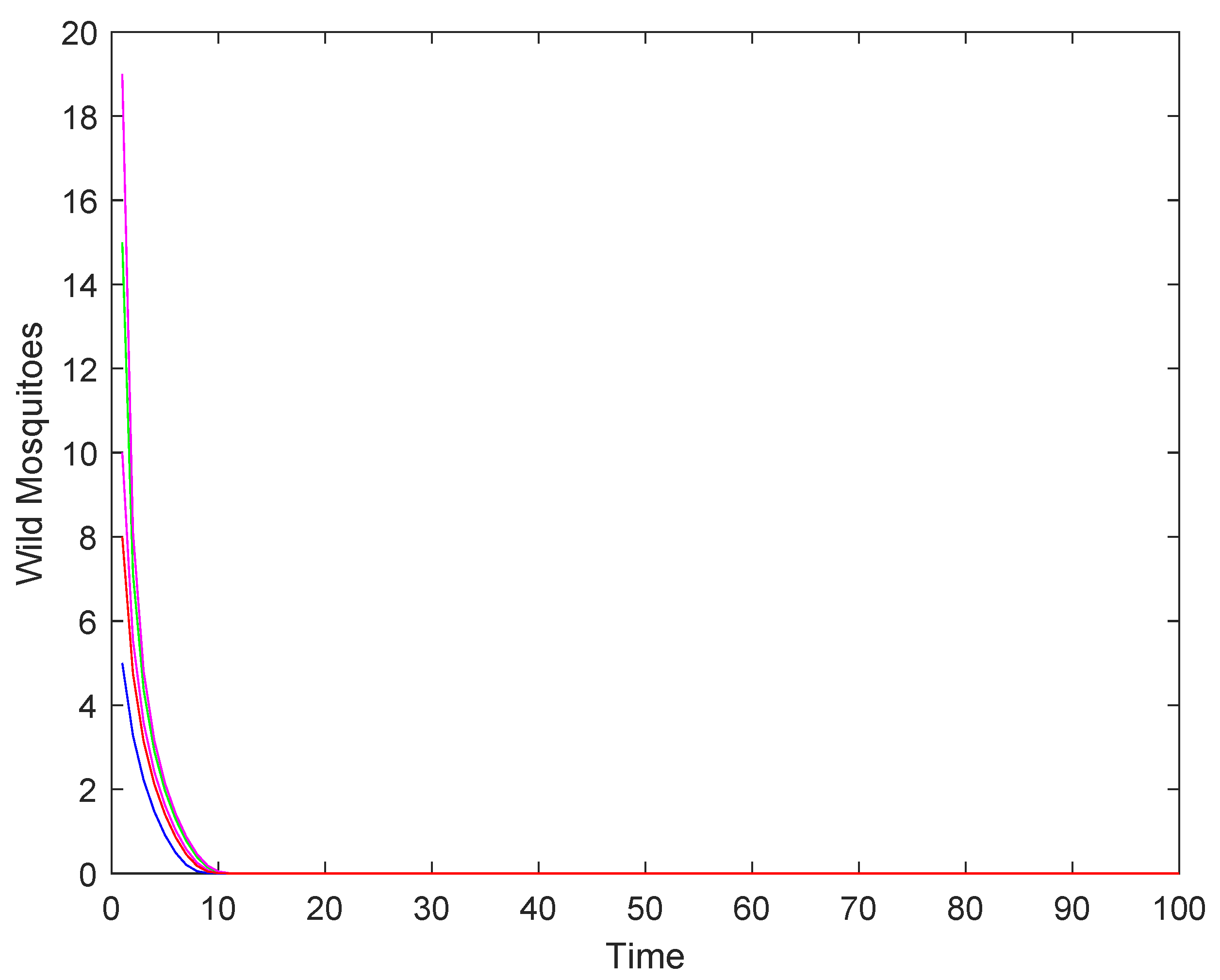
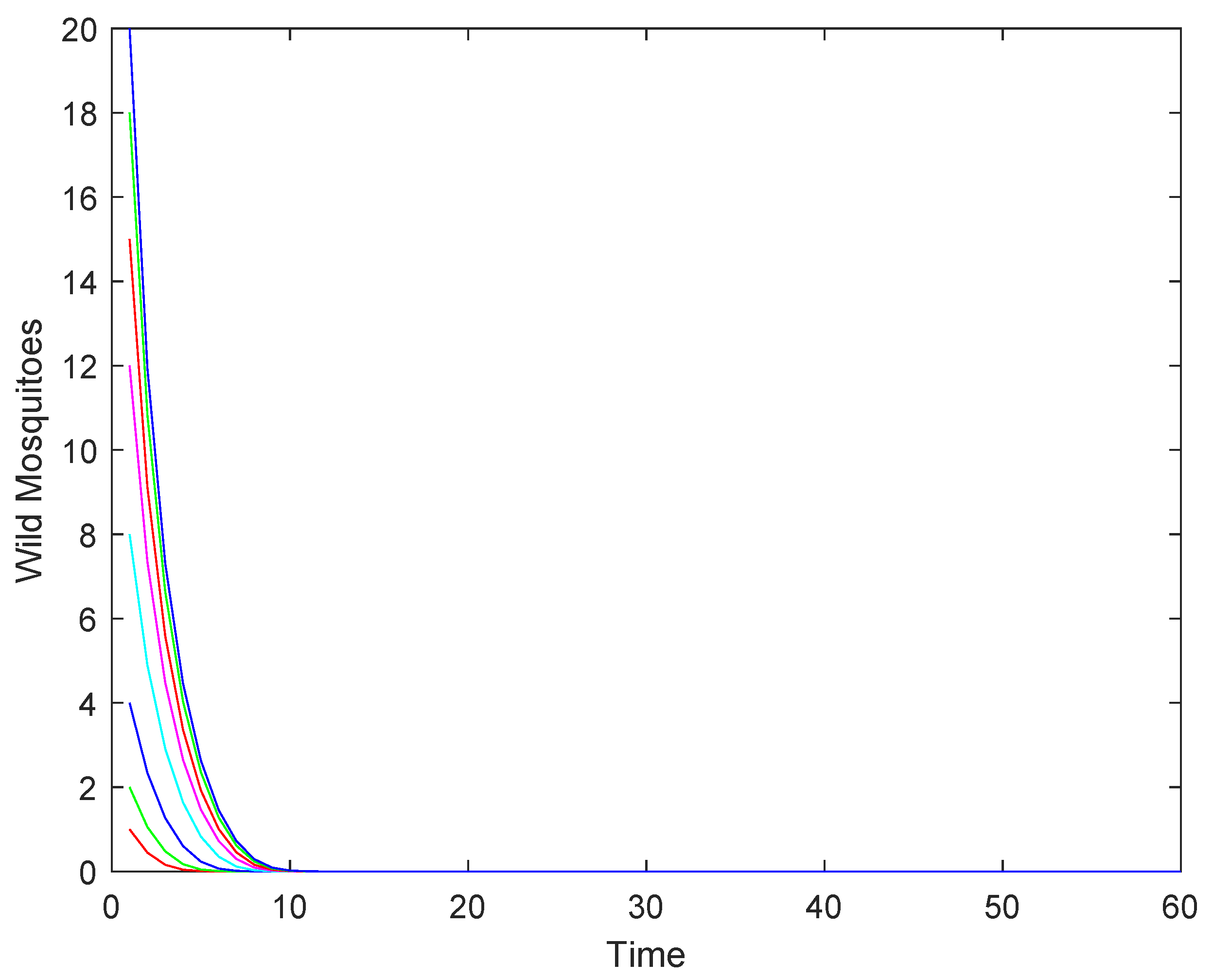
When the intrinsic growth rate $r_0<1$, the wild mosquito population will eventually decline to extinction, regardless of the initial population size. This indicates that the population cannot sustain itself under these conditions.

(2)

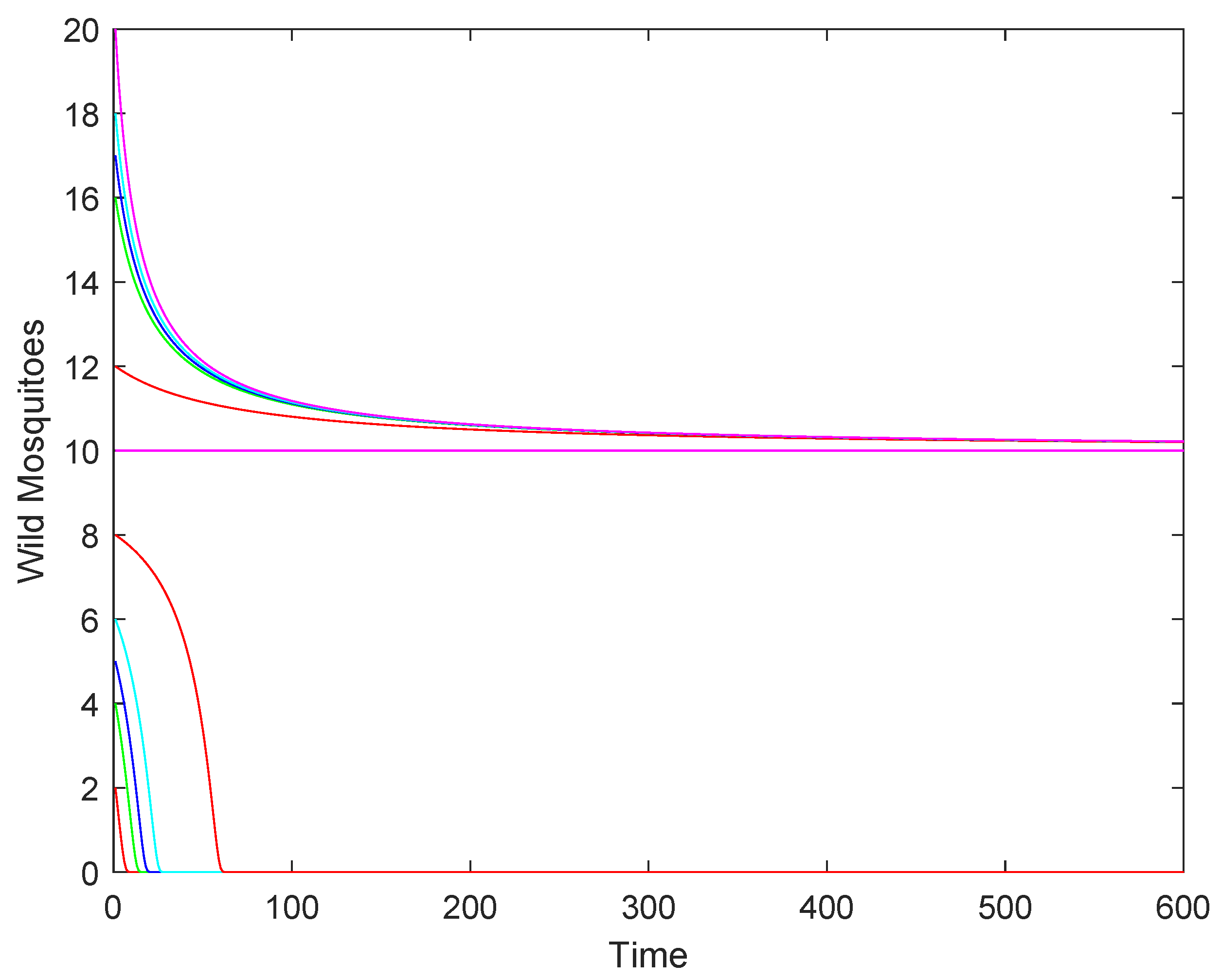
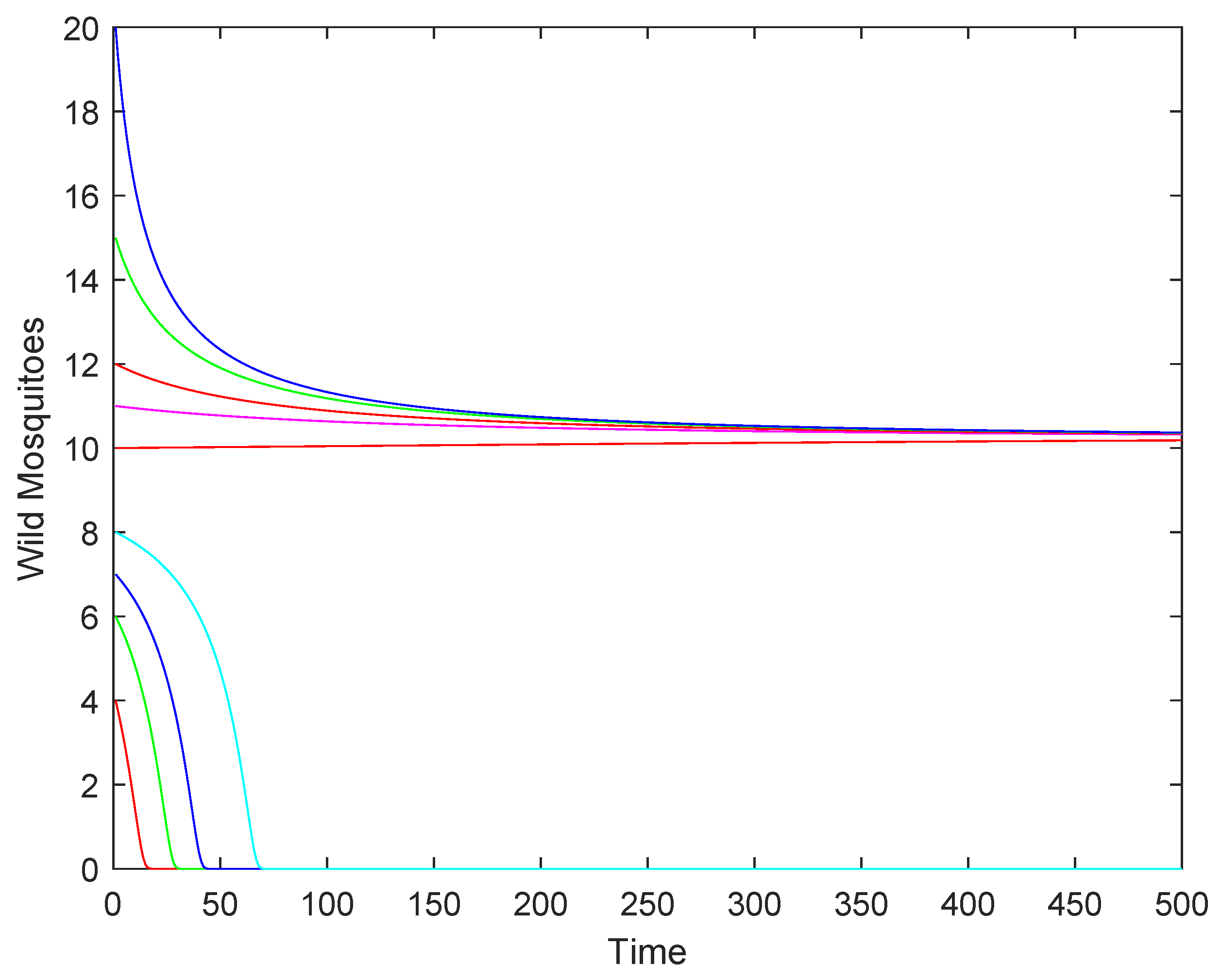
When the intrinsic growth rate $r_0=1$, the population may either stabilize at the equilibrium $M_1^{*}$ or decline to extinction, depending on whether the initial population size is above or below $M_1^{*}$. This represents a critical threshold where the population’s fate is determined by its starting size.

(3)

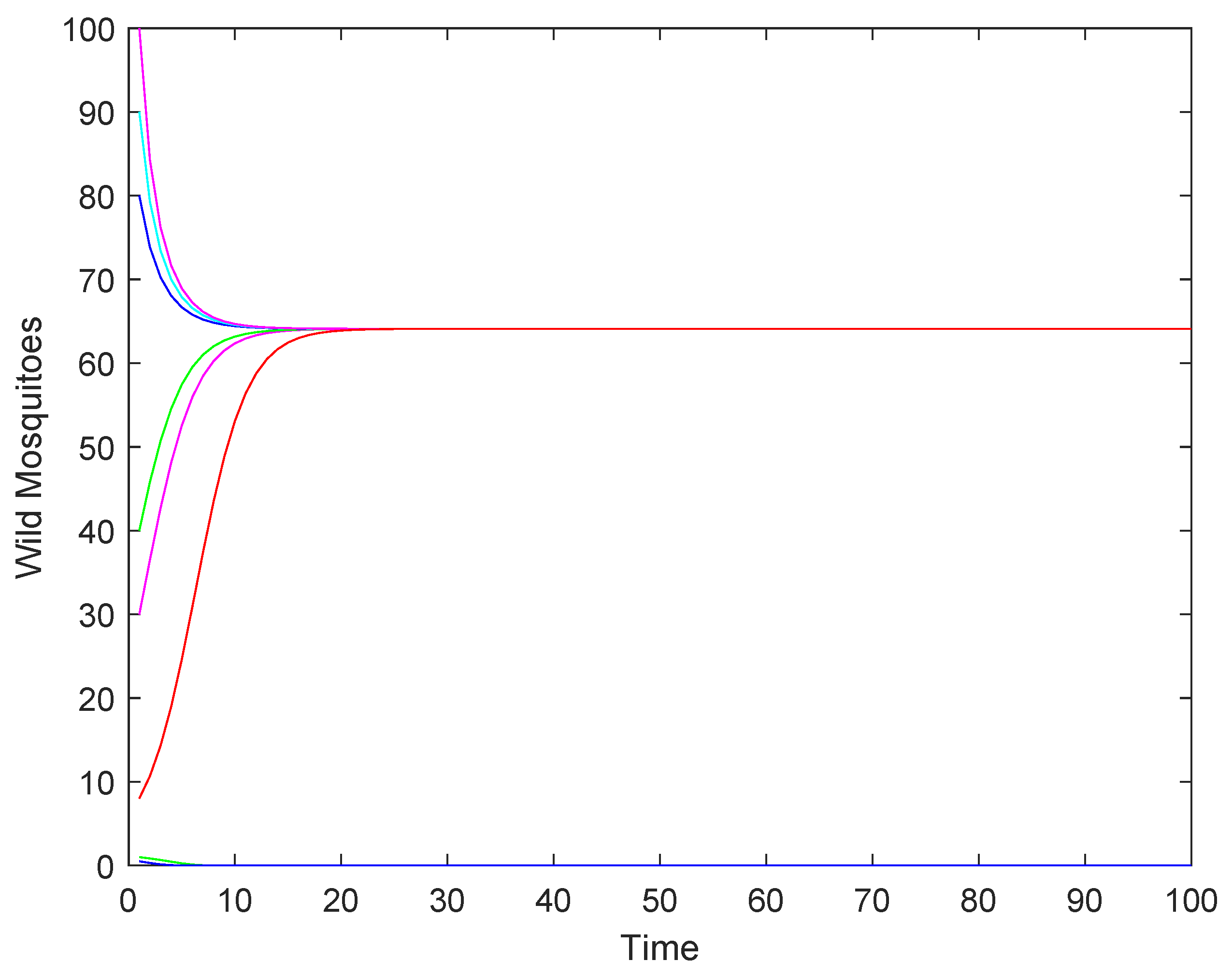
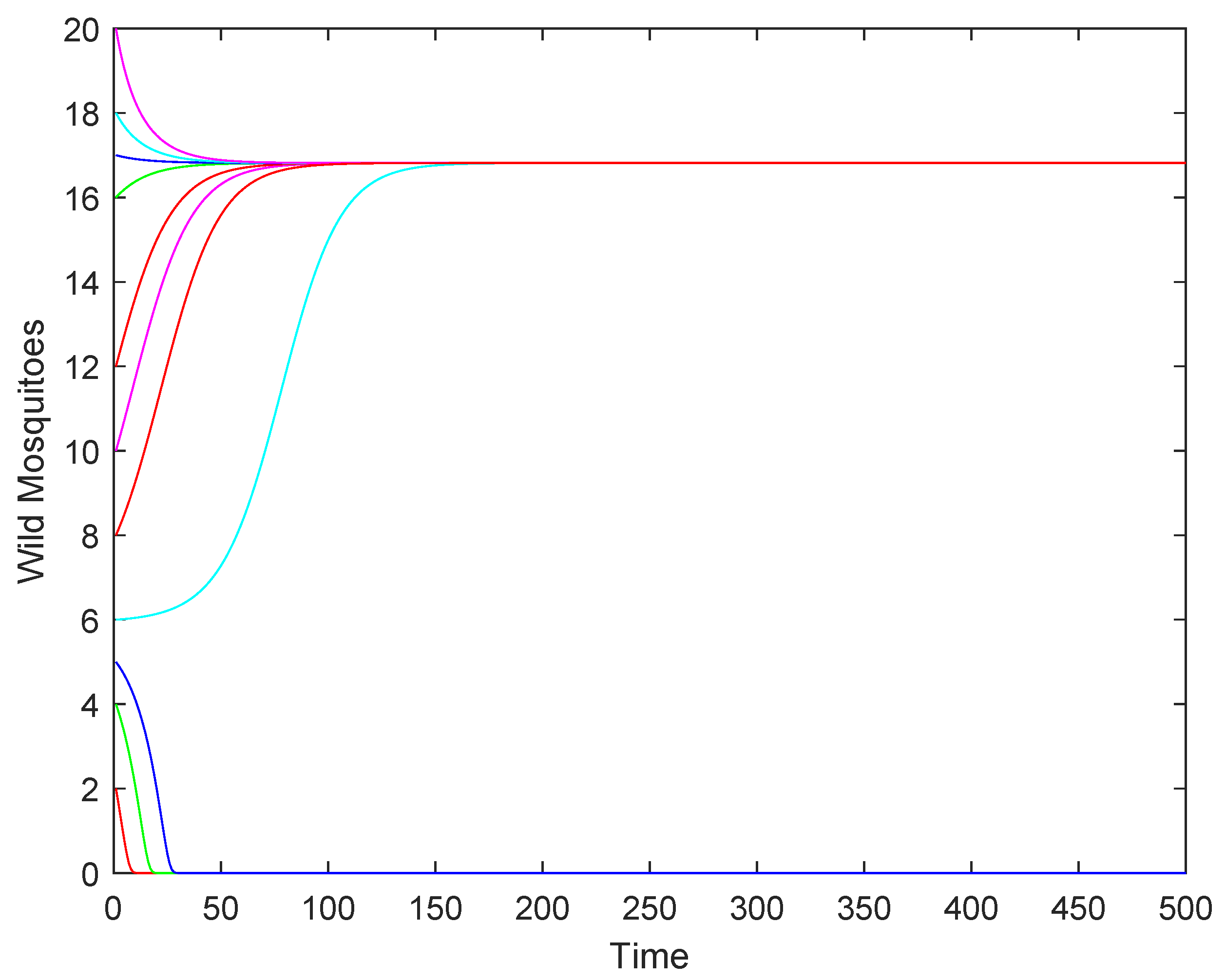
When the intrinsic growth rate $r_0>1$: if the initial population size is above $M_1^{-}$, the population will stabilize at the equilibrium $M_1^{+}$; if the initial population size is below $M_1^{-}$, the population will decline to extinction.

2.2. Numerical Simulations

In this subsection, we present a few specific examples and use numerical simulations to verify the validity of the conclusions drawn above.

Firstly, we choose the following parameters:

$$\eta =0.1,\mu =0.1,a=1,k=1,\sigma =1.$$

It can be calculated that $r_0\approx 0.6414<1$. According to Theorem 2, model (2) does not have a positive fixed point, and the only fixed point, $M=0$, is globally asymptotically stable (see Figure 1).

Next, we select the parameters:

$$\eta =0.01,\mu =0.1,a=1.21,k=0.9,\sigma =1.$$

In this case, $r_0=1$. As shown in Figure 2, besides the zero fixed point, model (2) also has a unique positive fixed point $M_1^{*}=10$. This fixed point is stable for values greater than it and unstable for values less than it, which is consistent with the conclusion of Theorem 2.

Finally, we choose the parameters:

$$\eta =0.01,\mu =0.1,a=1.5,k=1,\sigma =1.$$

The calculation gives $r_0\approx 1.3774>1$, and the model (2) has two positive fixed points, $M_1^{+}\approx 64.1068$ and $M_1^{-}\approx 1.5599$. From Figure 3, we observe that the larger positive fixed point $M_1^{+}$ is asymptotically stable in the interval $(M_1^{-},\infty )$, the zero fixed point is asymptotically stable in the interval $(0,M_1^{-})$, and the model (2) is bistable. This is also consistent with the conclusion of Theorem 2.

3. Constant Release of Sterile Mosquitoes

Taking into account the release of sterile mosquitoes into the wild, we focus solely on sterile mosquitoes with mating capabilities. We assume that when previously released sterile mosquitoes lose their ability to mate, new sexually active sterile mosquitoes will be released into the field.

Following the traditional modeling approach, let $g_n$ represent the number of sterile mosquitoes in the environment at time point n, and let $C\left(g_n\right)$ represent the specific number released at time n. Since the time step in the model no longer directly corresponds to the life cycle or generation, we need to account for the mortality or survival rate of sterile mosquitoes at each time step. Therefore, it is necessary to introduce an equation that specifically describes the dynamics of sterile mosquitoes in the model

$$g_{n+1}=(C\left(g_n\right)+g_n)S_g\left(g_n\right),$$

(7)

where $S_g\left(g_n\right)$ denotes the probability that a sterile mosquito survives from time n to $n+1$. In this way, the dynamic process of sterile mosquitoes is incorporated into the model.

It is worth noting that some previous studies [5,8,9,10] focus solely on sterile mosquitoes during their sexually active period when constructing the model. These studies assume that the mortality rate of these mosquitoes during this period can be neglected, given the relatively short duration of their sexual activity. In this case, the number of sterile mosquitoes at time n is directly given by a predefined non-negative function, and there is no need for a special dynamic equation for sterile mosquitoes.

Based on this idea, we construct a simplified model that only includes wild mosquitoes. For simplicity, we further assume that the number of sterile mosquitoes remaining sexually active in the field is constant at a certain positive value $c>0$. In other words, an equal number of new sexually active sterile mosquitoes are released each time a previously released sterile mosquito loses its ability to mate. Therefore, we have

$$g_n=c.$$

Since $M_n$ represents the number of adult mosquitoes in the wild, and the survival probability is assumed to be independent of density, the addition of sterile mosquitoes only affects the breeding period. Thus, the birth-rate function can be rewritten as

$$A\left(M_n\right)={\displaystyle \frac{a{M}_n}{\sigma +M_n}}·{\displaystyle \frac{M_n}{c+M_n}}.$$

The dynamics of the interaction between wild and sterile mosquitoes can be described by the following model

$$M_{n+1}={\displaystyle \frac{ak{M}_n^3}{\left(\sigma +M_n\right)\left(1+\eta M_n\right)\left(c+M_n\right)}}+\mu M_n.$$

(8)

In the following, we primarily focus on the analysis of model (8), which describes the constant release of sterile mosquitoes. We will discuss the existence and stability of its fixed points and analyze the related results.

3.1. The Existence and Stability of Fixed Points

First, let us determine the existence of fixed points for the model (8). To this end, we define the function on the right-hand side of (8) as follows:

$$G(M_n,c):={\displaystyle \frac{ak{M}_n^3}{\left(\sigma +M_n\right)\left(1+\eta M_n\right)\left(c+M_n\right)}}+\mu M_n.$$

(9)

Thus, Equation (8) can be rewritten as:

$$\Delta \left(M_n\right)=-{\displaystyle \frac{g_3\left(M_n,c\right)}{g_1\left(M_n,c\right)}}=-M_n+G\left(M_n,c\right),$$

(10)

where

$$g_1(M,c)=\left(\sigma +M\right)\left(1+\eta M\right)\left(c+M\right),$$

$$g_2(M,c)=(1-\mu )M{g}_1(M,c)-ak{M}^3,$$

$$g_3(M,c)=g_1(M,c)\left[M-G(M,c)\right].$$

Simplifying further, we obtain

$${\displaystyle \frac{1}{(1-\mu )M}}{g}_3(M,c)=\eta M^3+\left(c\eta +\sigma \eta +1-{\displaystyle \frac{ak}{1-\mu }}\right)M^2+\left(c+\sigma +c\sigma \eta \right)M+c\sigma .$$

For convenience, let

$$B=c\eta +\sigma \eta +1-{\displaystyle \frac{ak}{1-\mu }},C=c+\sigma +c\sigma \eta >0.$$

Then, we have

$${\displaystyle \frac{1}{(1-\mu )M}}{g}_2(M,c)=\eta M^3+B{M}^2+CM+c\sigma .$$

Therefore, the dynamics of the model (8) depend on the roots of the cubic form $g_2(M,c)$. The model’s dynamics are determined by the initial values and the zeros of $g_2(M,c)$. Thus, the next step is to analyze

$$g_2(M,c)=\eta M^3+B{M}^2+CM+c\sigma .$$

For any $c>0$, we have

$$g_2(0,c)=c\sigma >0,$$

and the derivative of $g_2(M,c)$ with respect to M is

$${g_2}^{\prime }\left(M,c\right)=3\eta M^2+2BM+C,$$

(11)

Let $D\left(g_2^{\prime }\right)=4B^2-12\eta C$ be the discriminant of the equation $g_2^{\prime }(M,c)=0$. Since $3\eta >0$ and $g_2^{\prime }(0,c)=C>0$, $g_2^{\prime }(M,c)$ has no positive roots when $B>0$. When $B<0$, i.e.,

$$c<{\displaystyle \frac{ak-(1-\mu )(1+\eta )}{(1-\mu )\eta }},$$

the derivative $g_2^{\prime }(M,c)$ has two positive roots

$$0<m_1={\displaystyle \frac{-2B-\sqrt{D\left(g_2^{\prime }\right)}}{6\eta }}<m_2={\displaystyle \frac{-2B+\sqrt{D\left(g_2^{\prime }\right)}}{6\eta }}.$$

In this case, $g_2(M,c)$ is monotonically increasing on the intervals $(0,m_1)$ and $(m_2,\infty )$, and monotonically decreasing on $(m_1,m_2)$. The function $g_2(M,c)$ achieves a local maximum at $g_2(M,m_1)$ and a local minimum at $g_2(M,m_2)$. Therefore, when $g_2(M,m_2)>0$, $g_2(M,c)$ has no positive roots; when $g_2(M,m_2)=0$, $g_2(M,c)$ has one positive root; when $g_2(M,m_2)<0$, $g_2(M,c)$ has two positive roots, $M_1^c<M_2^c$, where $g(M_1^c,c)=g(M_2^c,c)=0$.

Next, we analyze the stability of the fixed points.

When $0<c<{\displaystyle \frac{ak-(1-\mu )(1+\eta )}{(1-\mu )\eta }}$, and $g_2(M,m_2)>0$, the equation $g_2^{\prime }(M,c)=0$ has two solutions, $m_1$ and $m_2$. Since $g_2^{\prime }(0,c)=C$, as mentioned earlier, the model (8) has two positive fixed points, $M_1^c$ and $M_2^c$. If $M_0<M_1^c$, then for all $n=1,2,\dots$, we have $M_n<M_1^c$. Otherwise, suppose that there exists $n_0\ge 1$ such that $M_n<M_1^c$ for $n=0,1,\dots ,n_0-1$, but $M_{n_0}>M_1^c$. From Equation (9), we know that $G(M,c)$ is strictly increasing with respect to both M and c. Therefore, we have

$$M_{n_0}=G(M_{n_0-1},c)<G(M_1^c,c)=M_1^{*},$$

which leads to a contradiction.

When $g_2(M_n,c)\in (0,M_1^c)$, $g_2(M_n,c)$ is positive. Therefore, if $M_0\in (0,M_1^c)$, from Equation (10) we can deduce that $M_n$ will monotonically decrease to 0.

Similarly, we can prove that when $M_0\in (M_1^c,M_2^c)$, for all $n=1,2,\dots$, we have $M_n\in (M_1^c,M_2^c)$. First, for $n=1,2,\dots$, let $M_n<M_2^c$. Otherwise, if there exists $n_0\ge 1$, for all $n=1,2,\dots ,n_0-1$ we have $M_n<M_2^c$, but $M_{n_0}>M_2^c$, then

$$M_{n_0}=G(M_{n_0-1},c)<G(M_2^c,c)=M_2^c,$$

which again leads to a contradiction.

When for all $n=1,2,\dots$, $M_n>M_1^c$, otherwise, if there exists $n_0\ge 1$, when $n=0,1,\dots ,n_0-1$, we have $M_n>M_1^c$, but $M_{n_0}<M_1^c$, then

$$M_{n_0}=G(M_{n_0-1},c)>G(M_1^c,c)=M_1^c,$$

which leads to a contradiction.

When $g_2(M_n,c)\in (M_1^c,M_2^c)$, we know that $g_2(M_n,c)$ is negative. Therefore, if $M_0\in (M_1^c,M_2^c)$, then $M_n$ will monotonically increase to $M_2^c$. $M_1^c$ is unstable, and similarly, for any $M_n>M_2^c$, we have $\Delta \left(M_n\right)<0$ and

$$M_{n+1}=G(M_n,c)>G(M_2^c,c)=M_2^c.$$

Thus, when $M_0>M_2^c$, $M_n$ will monotonically decrease to $M_2^c$.

When $0<c<{\displaystyle \frac{ak-(1-\mu )(1+\eta )}{(1-\mu )\eta }}$ and $g_2(M,m_2)=0$, model (8) has a positive fixed point $M_{*}^c$. From Equation (10), we know that for any $M_n\in (0,M_c^{*})$, we have $\Delta \left(M_n\right)<0$ and

$$M_{n+1}=G(M_n,c)>G(M_c^{*},c)=M_c^{*}.$$

If $M_0\in (0,M_c^{*})$, then $M_n$ will monotonically decrease to 0. Similarly, for any $M_n>M_c^{*}$, we have $\Delta \left(M_n\right)<0$ and

$$M_{n+1}=G(M_n,c)>G(M_3^{*},c)=M_3^{*}.$$

This means that for any $M_0>M_c^{*}$, $M_n$ will monotonically decrease to $M_c^{*}$.

In summary, when ${\displaystyle 0<c<\frac{ak-\left(1-\mu \right)\left(1+\eta \right)}{\left(1-\mu \right)\eta }}$, we can draw the following conclusions.

Theorem 3. 

(1)  If $g_2(M,m_2)>0$, then model (8) does not have a positive fixed point. The trivial fixed point is globally asymptotic stable.

(2) 

If $g_2(M,m_2)=0$, then model (8) has a unique positive fixed point $M_{*}^c$ which is semi-stable.

(3) 

If $g_2(M,m_2)<0$, then model (8) has two positive fixed points $0<M_1^c<M_2^c$. The fixed point $M_1^c$ is unstable, while $M_2^c$ is locally asymptotically stable on $(M_1^c,\infty )$; The trivial fixed point is locally asymptotically stable on $(0,M_1^c)$.

From Theorem 3, we observe that when the constant release amount c satisfies $0<c<{\displaystyle \frac{ak-(1-\mu )(1+\eta )}{(1-\mu )\eta }}$, the following outcomes are possible for the wild mosquito population:

(1)

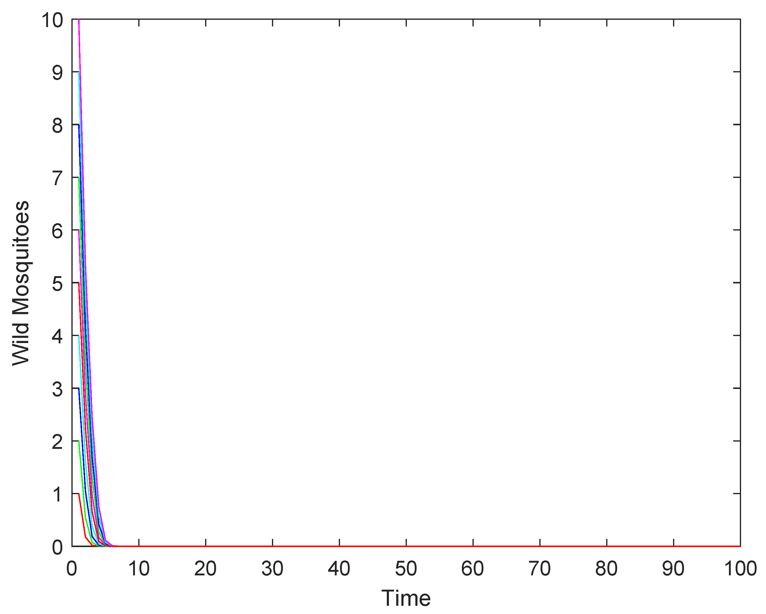
If $g_2(M,m_2)>0$, the wild mosquito population will eventually be eradicated. This indicates that the sterile mosquito release strategy is effective in driving the population to extinction.

(2)

If $g_2(M,m_2)=0$, the population may either stabilize at the equilibrium $M_{*}^c$ or decline to extinction, depending on the initial population size. This represents a critical scenario where the success of eradication depends on the starting conditions.

(3)

If $g_2(M,m_2)<0$: when the initial population size is above $M_1^c$, the population will stabilize at the higher equilibrium $M_2^c$, while when the initial population size is below $M_1^c$, the population will decline to extinction.

3.2. Numerical Simulations

Here are a few specific examples, where numerical simulations are used to verify the correctness of the above conclusions.

First, we choose the parameters $a=2$, $k=1$, $\mu =0.1$, $\sigma =1$, and $\eta =0.1$. The calculation yields $Z\approx 11.222$. We then set the parameter $c=11$ (with $c<Z$) and find that $g_2(M,m_2)>0$. As shown in Figure 4, there is no positive fixed point in the difference Equation (8), and the zero fixed point is globally asymptotically stable.

Next, we keep the other parameters unchanged and set $c=6$ (with $c<Z\approx 11.222$) and $g_2(M,m_2)=0$. According to Theorem 3, the difference Equation (8) has a unique positive fixed point, which is semi-stable (see Figure 5).

To further reduce the release parameter, we take $c=1$ (with $c<Z\approx 11.222$) and $g_2(M,m_2)<0$. In this case, the difference Equation (8) has two positive fixed points: $M_1^c\approx 3.5858$ and $M_2^c\approx 7.0309$. As shown in Figure 6, we observe that the positive fixed point $M_1^c$ is unstable, $M_2^c$ is locally asymptotically stable for $M\in (M_1^c,\infty )$, and the zero fixed point is locally asymptotically stable for $M\in (0,M_1^c)$. Therefore, the model (8) is bistable.

4. Proportional Release of Sterile Mosquitoes

The constant release strategy maintains a fixed number of sexually active sterile mosquitoes in the environment, regardless of fluctuations in the wild mosquito population. While this approach is simple and cost effective, it may lead to inefficiencies, such as excessive releases when wild mosquito numbers are already low.

To address this, we propose a proportional release strategy, where the number of sterile mosquitoes is adjusted based on the wild mosquito population to maintain a fixed ratio. This method offers more precise control by dynamically responding to population changes, ensuring effective competition for mating opportunities and reducing the reproductive capacity of wild mosquitoes.

When the number of wild mosquitoes in the environment is in a certain proportion to the number of sterile mosquitoes, let us assume $g_n=b{M}_n$, and the birth-rate function can be written as

$$A\left(M_n\right)={\displaystyle \frac{a{M}_n}{\sigma +M_n}}{\displaystyle \frac{M_n}{b{M}_n+M_n}}.$$

The dynamics of the interaction between wild mosquitoes and sterile mosquitoes can be described by the following difference equation

$$M_{n+1}={\displaystyle \frac{ak{M}_n^3}{\left(\sigma +M_n\right)\left(1+\eta M_n\right)\left(1+b\right)M_n}}+\mu M_n.$$

(12)

Obviously, the above equation can be simplified as

$$M_{n+1}={\displaystyle \frac{ak{M}_n^2}{\left(\sigma +M_n\right)\left(1+\eta M_n\right)\left(1+b\right)}}+\mu M_n.$$

(13)

4.1. The Existence and Stability of Fixed Points

It is evident that Equation (13) always has a trivial fixed point.

To analyze the existence of a positive fixed point in Equation (13), if such a fixed point exists, the following equation must hold

$${\displaystyle \frac{M_n\left[ak{M}_n-(1-\mu )(\sigma +M_n)(1+\eta M_n)(1+b)\right]}{(\sigma +M_n)(1+\eta M_n)(1+b)}}=0,$$

(14)

which simplifies to

$$(1-\mu )(\sigma +M_n)(1+\eta M_n)(1+b)-ak{M}_n=0.$$

(15)

Expanding the above equation results in

$$(1-\mu )(1+b)\eta M_n^2-\left[ak-(1-\mu )(1+b)(1+\sigma \eta )\right]M_n+(1-\mu )(1+b)\sigma =0.$$

The existence of positive fixed points requires the discriminant of Equation (15) to be non-negative:

$$\begin{array}{cc}\hfill {\Delta }_b& ={\left[ak-(1-\mu )(1+b)(1+\eta \sigma )\right]}^2-4{(1-\mu )}^2{(1+b)}^2\eta \sigma \hfill \\ \hfill & =\left[ak-(1-\mu )(1+b)(1+\eta \sigma )+2(1-\mu )(1+b)\sqrt{\eta \sigma }\right]\hfill \\ \hfill & ·\left[ak-(1-\mu )(1+b)(1+\eta \sigma )-2(1-\mu )(1+b)\sqrt{\eta \sigma }\right]\hfill \\ \hfill & =\left[(1-\mu )(1+b)\left(-(1+\eta \sigma )+2\sqrt{\eta \sigma }\right)+ak\right]\hfill \\ \hfill & ·\left[(1-\mu )(1+b)\left(-(1+\eta \sigma )-2\sqrt{\eta \sigma }\right)+ak\right]\hfill \\ \hfill & =\left[ak-(1-\mu )(1+b){(1-\sqrt{\eta \sigma })}^2\right]·\left[ak-(1-\mu )(1+b){(1+\sqrt{\eta \sigma })}^2\right]\ge 0.\hfill \end{array}$$

Thus, model (9) has one or two positive solutions if and only if

$$ak\ge (1-\mu )(1+b){(1+\sqrt{\eta \sigma })}^2.$$

To further analyze the existence of positive fixed points, we define the threshold

$$b^{*}={\displaystyle \frac{ak}{(1-\mu ){(1+\sqrt{\eta \sigma })}^2}}-1.$$

Based on this threshold, we obtain:

When $b>b^{*}$, model (13) has no positive fixed points.

When $b=b^{*}$, model (13) has a unique positive fixed point

$$M_b^{*}={\displaystyle \frac{ak-(1-\mu )(1+b)(1+\eta \sigma )}{2\eta (1-\mu )(1+b)}}.$$

When $b<b^{*}$, model (13) has two positive fixed points

$$M_b^{\pm }={\displaystyle \frac{ak-(1-\mu )(1+b)(1+\eta \sigma )\pm \sqrt{{\Delta }_b}}{2\eta (1-\mu )(1+b)}}.$$

Next, we analyze the stability of the fixed points of model (13).

It is straightforward to verify that

$$\begin{array}{cc}\hfill & {\displaystyle \frac{d}{dM}}\left({\displaystyle \frac{ak{M}^2}{\left(\sigma +M\right)\left(1+\eta M\right)\left(1+b\right)}}+\mu M\right){|}_{M=0}\hfill \\ \hfill & =\left({\displaystyle \frac{2akM\left(\sigma +M\right)\left(1+\eta M\right)\left(1+b\right)-\left(2\eta M+1+\sigma \eta \right)ak{M}^2}{{\left(\sigma +M\right)}^2{\left(1+\eta M\right)}^2{\left(1+b\right)}^2}}+\mu \right){|}_{M=0}\hfill \\ \hfill & =\mu <1.\hfill \end{array}$$

From this, it follows that the travial fixed point is locally asymptotically stable.

Suppose $b<b^{*}$, where two positive fixed points $M_b^{\pm }$ exist. By substituting them into the difference Equation (13) and performing direct calculations, we obtain the following differential formula

$$\begin{array}{cc}\hfill M_{n+1}-M_n& ={\displaystyle \frac{ak{M}_n^2}{(\sigma +M_n)(1+\eta M_n)(1+b)}}+(\mu -1)M_n\hfill \\ & ={\displaystyle \frac{ak{M}_n^2+(\mu -1)(\sigma +M_n)(1+\eta M_n)(1+b)M_n}{(\sigma +M_n)(1+\eta M_n)(1+b)}}\hfill \\ & ={\displaystyle \frac{(\mu -1)(1+b)\left[\eta M_n^3+\left(\frac{ak}{(\mu -1)(1+b)}+1+\sigma \eta \right)M_n^2+\sigma M_n\right]}{(\sigma +M_n)(1+\eta M_n)(1+b)}}\hfill \\ & ={\displaystyle \frac{-\eta (1-\mu )M_n(M_n-M_b^{+})(M_n-M_b^{-})}{(\sigma +M_n)(1+\eta M_n)(1+b)}}.\hfill \end{array}$$

Thus, for all $n\ge 1$, we have: if $M_n<M_b^{-}$ or $M_n>M_b^{+}$, then $M_{n+1}<M_n$; if $M_n=M_b^{-}$ or $M_n=M_b^{+}$, then $M_{n+1}=M_n$; if $M_b^{-}<M_n<M_b^{+}$, then $M_{n+1}>M_n$. Therefore, all solution sequences are monotonic.

Furthermore, from (14), we derive

$$\begin{array}{cc}\hfill & M_{n+1}-M_b^{+}=M_{n+1}-M_n+M_n-M_b^{+}\hfill \\ \hfill & ={\displaystyle \frac{-\eta \left(1-\mu \right)M_n(M_n-M_b^{+})\left(M_n-M_b^{-}\right)}{\left(\sigma +M_n\right)\left(1+\eta M_n\right)}}+\left(M_n-M_b^{+}\right)\hfill \\ \hfill & =\left({\displaystyle \frac{-\eta \left(1-\mu \right)\left(M_n-M_b^{-}\right)M_n}{\left(\sigma +M_n\right)\left(1+\eta M_n\right)}}+1\right)\left(M_n-M_b^{+}\right)\hfill \\ \hfill & ={\displaystyle \frac{M_n-M_b^{+}}{\left(\sigma +M_n\right)\left(1+\eta M_n\right)}}\left[\eta M_n\left(\mu -1\right)\left(M_n-M_b^{-}\right)+\left(\sigma +M_n\right)\left(1+\eta M_n\right)\right]\hfill \\ \hfill & ={\displaystyle \frac{M_n-M_b^{+}}{\left(\sigma +M_n\right)\left(1+\eta M_n\right)}}\left[M_n\left(\sigma \eta +1+\left(\eta \left(\mu -1\right)+\eta \right)M_n-\eta \left(\mu -1\right)M_b^{-}\right)+\sigma \right]\hfill \\ \hfill & ={\displaystyle \frac{M_n-M_b^{+}}{\left(\sigma +M_n\right)\left(1+\eta M_n\right)}}\left[M_n\left(\sigma \eta +1+\mu \eta M_n+\left(1-\mu \right)\eta M_b^{-}\right)+\sigma \right].\hfill \end{array}$$

Thus, if $M_b^{-}<M_n<M_b^{+}$, then $M_b^{-}<M_{n+1}<M_b^{+}$; if $M_n>M_b^{+}$, then $M_{n+1}>M_b^{+}$. Similarly, we have

$$M_{n+1}-M_b^{-}={\displaystyle \frac{M_n-M_b^{-}}{(\sigma +M_n)(1+\eta M_n)}}\left[M_n(\sigma \eta +1+\mu \eta M_n+(1-\mu )\eta M_b^{+})+\sigma \right].$$

From the above analysis, it is evident that $M_b^{-}$ is unstable since any solution sequence will move away from $M_b^{-}$ regardless of whether the initial condition is above or below it. In contrast, $M_b^{+}$ is locally asymptotically stable. In fact, since all solution sequences $\left\{M_n\right\}$ are monotonic, any sequence starting from $M_1>M_b^{+}$ will monotonically decrease and converge to $M_b^{+}$. Similarly, if $M_b^{-}<M_1<M_b^{+}$, then ${lim}_{n\to \infty }{M}_n=M_b^{+}$, confirming the local asymptotic stability of $M_b^{+}$.

If $b=b^{*}$, the model has a unique positive fixed point $M_b^{*}$. From the earlier derivations, for all $n\ge 1$, we have

$$M_{n+1}-M_n=-{\displaystyle \frac{(1-\mu )(1+b)\eta M_n{(M_n-M_b^{*})}^2}{(\sigma +M_n)(1+\eta M_n)(1+b)}}<0.$$

Therefore, if $M_1>M_b^{*}$, the solution sequence $\left\{M_n\right\}$ monotonically decreases and converges to $M_b^{*}$; if $M_1<M_b^{*}$, the solution sequence $\left\{M_n\right\}$ moves away from $M_b^{*}$. Hence, the fixed point $M_b^{*}$ is semi-stable.

Based on the above analysis, we summarize the following conclusions regarding model (13):

Theorem 4. 

Let $b^{*}={\displaystyle \frac{ak}{(1-\mu ){(1+\sqrt{\eta \sigma })}^2}}-1$). Then,

(1) 

If $b>b^{*}$, then model (13) has no positive fixed points, and the trivial fixed point is globally asymptotically stable.

(2) 

If $b=b^{*}$, then model (13) has a unique positive fixed point $M_b^{*}$, which is semi-stable.

(3) 

If $b<b^{*}$, then model (13) has two positive fixed points, $M_b^{-}$ and $M_b^{+}$, where the fixed point $M_b^{-}$ is unstable, while $M_b^{+}$ is locally asymptotically stable on $(M_b^{-},\infty )$. The trivial fixed point is locally asymptotically stable on $(0,M_b^{-})$.

From Theorem 4, we can see that if the release rate b is sufficient large ($b>b^{*}$), the wild mosquito population will eventually be eradicated, regardless of the initial population size. In addition, if $b=b^{*}$ or $b<b^{*}$, the population may either stabilize at certain level ($M_b^{*}$ or $M_b^{+}$) or decline to extinction, depending on the initial conditions.

From Theorem 4, we observe the following outcomes for the wild mosquito population under different release rates b:

(1)

If the release rate b is sufficiently large ($b>b^{*}$), the wild mosquito population will eventually be eradicated, regardless of the initial population size. This indicates that a high release rate of sterile mosquitoes can effectively suppress and eliminate the wild population.

(2)

If the release rate b equals the threshold ($b=b^{*}$), the population may either stabilize at the equilibrium $M_b^{*}$ or decline to extinction, depending on the initial population size. This represents a critical scenario where the success of eradication depends on the starting conditions.

(3)

If the release rate b is below the threshold ($b<b^{*}$), the population may either stabilize at the higher equilibrium $M_b^{+}$ or decline to extinction, depending on whether the initial population size is above or below a certain threshold.

4.2. Numerical Simulations

In this subsection, we analyze the dynamic behavior of the difference Equation (13) under various parameter settings through numerical simulations, with a particular focus on the stability characteristics and changes in the fixed points.

First, consider the parameter values: $a=1$, $k=1$, $\mu =0.2$, $\eta =0.01$, and $\sigma =1$. Under these conditions, numerical analysis yields an approximate parameter threshold value of $b^{*}\approx 0.033$. When $b=1$, i.e., $b>b^{*}$, the difference Equation (13) has no positive fixed points, and the trivial fixed point is globally asymptotically stable (see Figure 7).

Next, when the value of b is set to the critical threshold, i.e., $b=0.033=b^{*}$, the dynamic behavior of the system changes, as illustrated in Figure 8. In this scenario, the system possesses a unique positive fixed point, $M_b^{*}$, which is semi-stable. Specifically, for certain initial values, the solution of the difference equation converges to this fixed point.

Finally, when $b=0.01<b^{*}$, Figure 9 demonstrates that the difference Equation (13) exhibits bistable behavior. In this case, the system has two positive fixed points, $M_b^{-}$ and $M_b^{+}$, where $M_b^{-}$ is unstable, and $M_b^{+}$ is locally asymptotically stable in the interval $(M_b^{-},\infty )$. Simultaneously, the trivial fixed point is locally asymptotically stable in the interval $(0,M_b^{-})$.

These numerical simulation results highlight the richness and complexity of the dynamic behavior of the difference Equation (13) under different parameter configurations, providing further validation of the preceding theoretical findings.

5. Conclusions

In this paper, we construct a novel discrete-time mosquito population model to analyze the interaction between wild and sterile mosquito populations within a broader environmental framework. A key feature of this model is its incorporation of a more generalized time-step concept, distinguishing it from many existing studies that typically rely on generational evolution or models focused on specific life cycle stages. In this study, we assume that the population survival rate follows a nonlinear Beverton–Holt type function, considering the influence of survival probability at each time step.

We begin by developing a homogeneous model that does not differentiate between the various life-cycle stages of individual mosquitoes. Through a preliminary analysis of the dynamic behavior of this base model—excluding the influence of sterile mosquitoes—we explore its fundamental dynamics. The model is then extended to incorporate the effects of sterile mosquitoes.

Firstly, considering that sterile mosquitoes may gradually lose their mating ability in practical applications, we introduce a release strategy whereby new sexually active sterile mosquitoes are introduced at appropriate intervals. This strategy aims to maintain a relatively stable population of sexually active sterile mosquitoes in the field, thereby achieving the objective of controlling wild mosquito populations.

Secondly, we explore another commonly used approach in which the release of sterile mosquitoes is adjusted based on the population size of wild mosquitoes. The advantage of this strategy lies in its ability to more precisely target the actual number of mosquitoes, effectively controlling mosquito fertility by maintaining a fixed ratio between sterile and wild mosquitoes, thus regulating their reproductive rate and overall population size.

On this basis, we investigate the dynamic behavior of the model, with a particular focus on the existence and stability of fixed points. This analysis not only provides a theoretical foundation for understanding population dynamics but also offers valuable insights for developing effective mosquito control strategies.

References

- Almeida, L.; Duprez, M.; Privat, Y.; Vauchelet, N. Optimal control strategies for the sterile mosquitoes technique. J. Differ. Equ. 2022, 311, 229–266. [Google Scholar] [CrossRef]
- Benedict, M.Q.; Robinson, A.S. The first releases of transgenic mosquitoes: An argument for the sterile insect technique. Trends Parasitol. 2003, 19, 349–355. [Google Scholar] [CrossRef] [PubMed]
- Stone, C.M. Transient population dynamics of mosquitoes during sterile male releases: Modelling mating behaviour and perturbations of life history parameters. PLoS ONE 2013, 8, e76228. [Google Scholar] [CrossRef] [PubMed]
- Bond, J.G.; Osorio, A.R.; Avila, N.; Gomez-Simuta, Y.; Marina, C.F.; Fernandez-Salas, I.; Liedo, P.; Dor, A.; Carvalho, D.O.; Bourtzis, K.; et al. Optimization of irradiation dose to Aedes aegypti and Ae. albopictus in a sterile insect technique program. PLoS ONE 2019, 14, e0212520. [Google Scholar] [CrossRef] [PubMed]
- Yu, J. Modeling mosquito population suppression based on delay differential equations. SIAM J. Appl. Math. 2018, 78, 3168–3187. [Google Scholar] [CrossRef]
- Zheng, X.; Zhang, D.; Li, Y.; Yang, C.; Wu, Y.; Liang, X.; Liang, Y.; Pan, X.; Hu, L.; Sun, Q.; et al. Incompatible and sterile insect techniques combined eliminate mosquitoes. Nature 2019, 572, 56–61. [Google Scholar] [CrossRef] [PubMed]
- Zheng, B.; Li, J.; Yu, J. One discrete dynamical model on the Wolbachia infection frequency in mosquito populations. Sci. China Math. 2022, 65, 1749–1764. [Google Scholar] [CrossRef]
- Yu, J.; Li, J. Dynamics of interactive wild and sterile mosquitoes with time delay. J. Biol. Dyn. 2019, 13, 606–620. [Google Scholar] [CrossRef] [PubMed]
- Yu, J. Existence and stability of a unique and exact two periodic orbits for an interactive wild and sterile mosquito model. J. Differ. Equ. 2020, 269, 10395–10415. [Google Scholar] [CrossRef]
- Yu, J.; Li, J. Global asymptotic stability in an interactive wild and sterile mosquito model. J. Differ. Equ. 2020, 269, 6193–6215. [Google Scholar] [CrossRef]
- Li, J. Modelling of transgenic mosquitoes and impact on malaria transmission. J. Biol. Dyn. 2011, 5, 474–494. [Google Scholar] [CrossRef]
- Li, J.; Yuan, Z. Modelling releases of sterile mosquitoes with different strategies. J. Biol. Dyn. 2015, 9, 1–14. [Google Scholar] [CrossRef] [PubMed]
- Yu, J.; Li, J. Discrete-time models for interactive wild and sterile mosquitoes with general time steps. Math. Biosci. 2022, 346, 108797. [Google Scholar] [CrossRef] [PubMed]
- Chen, L.S. Mathematical Ecology Modelling and Research Methods; Science Press: Beijing, China, 1988. (In Chinese) [Google Scholar]
Disclaimer/Publisher’s Note: The statements, opinions and data contained in all publications are solely those of the individual author(s) and contributor(s) and not of MDPI and/or the editor(s). MDPI and/or the editor(s) disclaim responsibility for any injury to people or property resulting from any ideas, methods, instructions or products referred to in the content. |
© 2025 by the authors. Licensee MDPI, Basel, Switzerland. This article is an open access article distributed under the terms and conditions of the Creative Commons Attribution (CC BY) license (https://creativecommons.org/licenses/by/4.0/).
Share and Cite
Hong, L.; Yang, Y.; Zhang, W.; Huang, M.; Zhou, X. Study on Discrete Mosquito Population-Control Models with Allee Effect. Axioms 2025, 14, 193. https://doi.org/10.3390/axioms14030193
Hong L, Yang Y, Zhang W, Huang M, Zhou X. Study on Discrete Mosquito Population-Control Models with Allee Effect. Axioms. 2025; 14(3):193. https://doi.org/10.3390/axioms14030193
Chicago/Turabian StyleHong, Liang, Yanhua Yang, Wen Zhang, Mingzhan Huang, and Xueyong Zhou. 2025. "Study on Discrete Mosquito Population-Control Models with Allee Effect" Axioms 14, no. 3: 193. https://doi.org/10.3390/axioms14030193
APA StyleHong, L., Yang, Y., Zhang, W., Huang, M., & Zhou, X. (2025). Study on Discrete Mosquito Population-Control Models with Allee Effect. Axioms, 14(3), 193. https://doi.org/10.3390/axioms14030193