An O(kn)-Time Algorithm to Solve Steiner (k, k′)-Eccentricity on Trees

Abstract

Steiner $(k,k^{\prime })$-eccentricity on a given fixed $k^{\prime }$-subset in a graph G is the maximum Steiner distance over all k-subsets of $V\left(G\right)$ which contain the fixed $k^{\prime }$-set, where the Steiner distance of a set is the size of a minimum Steiner tree on this set in a graph. Let $R\subseteq V\left(T\right)$ be the given fixed $k^{\prime }$-subset in a tree T. Let $k_1$ and $k_2$ be two integers such that $k_1\ge k_2\ge k^{\prime }$. We prove that, in a tree, every optimal solution of Steiner $(k_1,k^{\prime })$-eccentricity on R takes some optimal solution of Steiner $(k_2,k^{\prime })$-eccentricity on R as a partial solution. On the other hand, every optimal solution of Steiner $(k_2,k^{\prime })$-eccentricity on R is part of some optimal solution of Steiner $(k_1,k^{\prime })$-eccentricity on the set R in a tree. Finally, we present an $O\left(kn\right)$-time algorithm to solve Steiner $(k,k^{\prime })$-eccentricity on a given fixed $k^{\prime }$-set in trees.

1. Introduction

The Steiner $(k,k^{\prime })$-eccentricity on a given fixed $k^{\prime }$-subset of vertices measures the maximum distance from the subset to all k-sets, each of which contains the subset. This metric reflects a kind of optimal connectivity challenge. This concept can engage in metaphorically multi-attribute decision-making (MADM) [1], where each attribute could represent a “vertex” and the optimization of the overall system’s performance corresponds to finding the “Steiner point” that maximizes “distance” to all objectives. The Steiner distance is the minimum number of edges in a connected subgraph that contains a given subset of vertices. This distance between two subsets is the distance for their union.

Particularly, if $k^{\prime }=1$, the Steiner $(k,k^{\prime })$-eccentricity turns to be Steiner k-eccentricity on a specific vertex. The research of Steiner k-eccentricity can be traced back to the 1990s [2]. Researchers have studied extensively mathematical properties of Steiner k-eccentricity [3,4,5,6,7]. Steiner k-eccentricity has indeed found practical applications. Huilgol et al. [4], in their 2024 study, applied Steiner k-eccentricity in predicting the boiling points of primary and secondary amines, demonstrating its effectiveness in chemical property prediction. In addition, it has been used to calculate network similarity measures [8]. Additionally, it is leveraged for predicting the molecular activity of substances [9]. Collectively, these advancements highlight the adaptability and significance of Steiner k-eccentricity as a tool in the fields of network analysis and chemical predictive modeling. For a given fixed $k^{\prime }$-set of vertices R, the Steiner $(k,k^{\prime })$-eccentricity on R is the maximum number of edges in a minimum distance Steiner tree with $k\ge k^{\prime }$ vertices and containing R. An optimal solution of this is a corresponding Steiner tree. When, as for us, the underlying graph is a tree, every Steiner tree is uniquely determined by, and is easily computed from by, any set of its vertices that includes all its leaves.

In decision making contexts, seeking a solution that optimizes across various attributes is to find a Steiner tree in a network of objectives, where the goal is to minimize the cumulative or maximum ’cost’ associated with achieving all objectives simultaneously. Since the well-known minimum Steiner tree problem has been proven to be NP-hard [10], it is not easy to compute Steiner $(k,k^{\prime })$-eccentricity. In recent years, algorithms for computing Steiner k-eccentricity have been developed [11]. Li et al. studied average Steiner 3-eccentricity on trees [12] and devised a polynomial algorithm [11] for finding the Steiner k-eccentricity of a given vertex in a tree. Later, Li et al. [13] tried to compute Steiner k-eccentricity on general graphs by using the algorithm on trees. But, the time-complexity is really unbearable.

In 2024, Gengji Li et al. delved into the realm of graph theory, specifically focusing on the Steiner $(3,2)$-eccentricity of a 2-set within trees in their research work [14]. This study not only explores this particular aspect of Steiner distances but also contributes by establishing several bounds—both lower and upper—for the average Steiner $(3,2)$-eccentricity on trees. Despite these advancements, computational studies and algorithmic developments for the broader concept of Steiner $(k,k^{\prime })$-eccentricity remain limited, indicating an area of future research where the practical computation and efficiency of such measures could be further investigated.

In this study, the structure of an optimal solution of Steiner $(k,k^{\prime })$-eccentricity on a fixed $k^{\prime }$-set in a tree is studied. For a given $k^{\prime }$-set $R\subseteq V\left(T\right)$ in a tree T and an integer $i:k^{\prime }\le i<k$, we prove that an optimal solution of Steiner $(k,k^{\prime })$-eccentricity on R takes some optimal solution of Steiner $(i,k^{\prime })$-eccentricity on R as a partial solution of it. In addition, given a subtree $T_1$ which is an optimal solution of Steiner $(k,k^{\prime })$-eccentricity on a fixed $k^{\prime }$-set R in a tree T, there is an optimal solution $T^{\ast }$ of Steiner $((k+1),k^{\prime })$-eccentricity on R such that $T^{\ast }$ contains the given $T_1$.

Finally, an $O\left(kn\right)$-time algorithm is devised to solve Steiner $(k,k^{\prime })$-eccentricity in a tree. The time complexity meets with the result in [11] for computing Steiner k-eccentricity.

The rest of this paper is organized as follows. Section 2 proposes basic terminologies and properties. We define and explore the concepts of quasi-pendent paths and the eccentricity of a subgraph in this section, which serve as foundational elements for the entire paper. The structural properties of optimal solutions are examined in Section 3. Particularly, Section 3 focuses on the relationship between Steiner $(k,k^{\prime })$-eccentricity and Steiner $((k-1),k^{\prime })$-eccentricity on a given fixed $k^{\prime }$-set. Section 4 shows that Steiner $(k,k^{\prime })$-eccentricity can be solved in $O\left(kn\right)$-time. We conclude the paper in Section 5 and propose several directions for future work.

2. Preliminary

In the remainder of this paper, we focus on trees and the underlying graph is always a tree. A tree is a connected graph which has no cycles. The vertex set and edge set of a tree T are, respectively, denoted as $V\left(T\right)$ and $E\left(T\right)$. If a tree is composed of a single vertex, then the tree is said to be trivial. If a tree contains more than one vertex, it is said to be non-trivial. The unique path between $v\in V\left(T\right)$ and $u\in V\left(T\right)$ in a tree T is denoted by $P_T(v,u)$. A vertex is a neighbor of another vertex if they are adjacent in a tree. The set of neighbors of a vertex v in a tree T is denoted as $Neighbo{r}_T\left(v\right)$. The degree of a vertex v in a tree T is denoted as $de{g}_t\left(v\right)$ which is the number of neighbors of v, i.e., $de{g}_T\left(v\right)=\left|Neighbo{r}_T\left(v\right)\right|$. If $de{g}_T\left(v\right)=1$, then v is said to be a leaf of T. The set of leaves in a tree T is denoted as $\mathit{\ell }\left(T\right)$. If $de{g}_T\left(v\right)=2$, then v is said to be an internal vertex of T. If $de{g}_T\left(v\right)>2$, then v is said to be a branching vertex or a branch of G. If G itself is a path, then a leaf of the path is also said to be an endpoint.

Let $V_1\subseteq V\left(T\right)$ and $E_1\subseteq E\left(T\right)$, respectively, be a subset of vertices and edges in a tree T. The induced subgraph of $V_1$ in T is denoted by $T\left[V_1\right]=(V_1,E^{\prime })$ which is a subgraph of T such that an edge of T is in $E^{\prime }$ if and only if its two endpoints are both in $V_1$. The induced subgraph of $E_1$ in T is denoted as $T\left[E_1\right]=(V^{\prime },E_1)$ which is a subgraph of T such that $V^{\prime }=V\left(E_1\right)$.

Lemma 1.

Let $T_1$ and $T_2$ be two sub-trees of a tree T such that $|V\left(T_1\right)\cap V\left(T_2\right)|\ge 2$. Let $u,v\in V\left(T_1\right)\cap V\left(T_2\right)$ be two distinct vertices. We have $V\left(P_T(u,v)\right)\subseteq V\left(T_1\right)\cap V\left(T_2\right)$.

Proof. 

Recall that the path P is unique, since T is a tree. Since $u,v\in V\left(T_1\right)$ and $T_1$ is connected, P must be a sub-tree of the tree $T_1$. In addition, $u,v\in V\left(T_2\right)$ and $T_2$ is connected, P must be a sub-tree of the tree $T_2$. So, P is a path both in $T_1$ and in $T_2$. Therefore, all vertices belonging to P are also in $V\left(T_1\right)\cap V\left(T_2\right)$.    □

Lemma 2.

Let $P_1$ and $P_2$ be two distinct paths in a tree T. If $E\left(P_1\right)\cap E\left(P_2\right)\ne \varnothing$ then the subgraph induced by $E\left(P_1\right)\cap E\left(P_2\right)$ is a single path in T.

Proof. 

Suppose on the contrary that the subgraph induced by common edges has more than one component. Obviously, each component is a sub-path of $P_1$, as well as $P_2$. Let p and $p^{\prime }$ be two different components. For the reason that T is connected, there exists two distinct sub-paths connecting p and $p^{\prime }$, respectively, in $P_1$ and $P_2$. This implies a cycle in the tree T.    □

The minimum Steiner tree on a set $S\subseteq V\left(T\right)$ in a tree T is denoted by $Stei\left(S\right)$. For us, the size of a tree is the number of edges in it. Each vertex in S is said to be a terminal vertex, while each vertex in $V\left(Stei\right(S\left)\right)\setminus S$ is said to be a Steiner vertex. The Steiner distance on a set S is the size of a $Stei\left(S\right)$, and is denoted as $d_T\left(S\right)$. A vertex set $S\subseteq V\left(T\right)$ is a k-set if $\left|S\right|=k$.

Lemma 3.

Let T be a tree and $S\subseteq V\left(T\right)$. The set of leaves in a minimum Steiner tree on S is a subset of S, i.e., $\mathit{\ell }\left(Stei\right(S\left)\right)\subseteq S$.

Proof. 

Any leaf not in S of a tree that connects S can be removed without disconnecting S. So, the leaves in a minimum Steiner tree of S should all belong to S.    □

Lemma 4.

Let $S\subseteq V\left(T\right)$ be a vertex set of a tree T. For every two vertices $u,v\in S$, the path $P_T(u,v)$ is contained by the minimum Steiner tree $Stei\left(S\right)$.

Proof. 

The path $P_T(u,v)$ is unique in the tree T. In addition, the vertex u and v should be connected in $Stei\left(S\right)$. So, the path $P_T(u,v)$ is contained in the minimum Steiner tree $Stei\left(S\right)$.    □

Given a fixed $k^{\prime }$-set $R\subseteq V\left(T\right)$ of a tree T, Steiner $(k,k^{\prime })$-eccentricity of R in T is defined as: ${ecc}_k(R,T)=max\{d_T\left(S\right):R\subseteq S\subseteq V\left(G\right),\left|R\right|=k^{\prime }\ge 0,\left|S\right|=k\ge k^{\prime }\}.$ If $\left|R\right|=0$, then $ec{c}_k(R,G)$ is defined to be zero. In this paper, we consider the case that $R\ne \varnothing$. If $\left|R\right|=1$, then Steiner $(k,1)$-eccentricity of R turns to be Steiner k-eccentricity of a given vertex. The computation of Steiner k-eccentricity on trees has been studied in paper [11,12].

Given a fixed $k^{\prime }$-set R, if S is a k-set such that $R\subseteq S$ and $\left|E\left(Stei\left(S\right)\right)\right|=ec{c}_k(R,T)$, then S is said to be a Steiner $(k,k^{\prime })$-ecc R-set corresponding to $Stei\left(S\right)$. The minimum Steiner tree $Stei\left(S\right)$ is an optimal solution corresponding to ${ecc}_k(R,T)$ and said to be a Steiner $(k,k^{\prime })$-ecc R-tree corresponding to S. In this paper, $T_R^k$ stands for a Steiner $(k,k^{\prime })$-ecc R-tree, and $S_R^k$ stands for a Steiner $(k,k^{\prime })$-ecc R-set.

Lemma 5.

Let $R\subseteq V\left(T\right)$ be a fixed $k^{\prime }$-set in a tree T. The Steiner tree $Stei\left(R\right)$ on R in T is a subgraph of $T_R^k$ for every $k\ge k^{\prime }$.

Proof. 

If $\left|R\right|=1$, then $Stei\left(R\right)$ is the single vertex in R. Obviously, $Stei\left(R\right)$ is a subgraph of a Steiner $(k,k^{\prime })$-ecc R-tree, for every $k\ge k^{\prime }$. The following proof considers the case that $\left|R\right|\ge 2$.

In order to prove that $Stei\left(R\right)$ is a subgraph of $T_R^k$, we need to prove $V\left(Stei\left(R\right)\right)\subseteq V\left(T_R^k\right)$. Because both $Stei\left(R\right)$ and $T_R^k$ are trees, by Lemma 1, $V\left(Stei\left(R\right)\right)\subseteq V\left(T_R^k\right)$ implies that $E\left(Stei\left(R\right)\right)\subseteq E\left(T_R^k\right)$. Since $R\subseteq V\left(Stei\right(R\left)\right)$ and $R\subseteq V\left(T_R^k\right)$, we are going to prove that $V\left(Stei\left(R\right)\right)\setminus R\subseteq V\left(T_R^k\right)$.

Suppose on the contrary that there is a vertex $v\in V\left(Stei\right(R\left)\right)\setminus R$ such that $v\notin V\left(T_R^k\right)$. Since $v\in Stei\left(R\right)\setminus R$, then there are two vertices $u,w\in R$ such that the path $P_{Stei\left(R\right)}(u,w)$ contains the vertex v. Because $v\notin V\left(T_R^k\right)$, $u\in V\left(T_R^k\right)$ and $w\in V\left(T_R^k\right)$, the path $P_{T_R^k}(u,w)$ does not go through v any more. Then, there are at least two different paths between u and w in the tree T, which is a contradiction. Therefore, $Stei\left(R\right)$ is a subgraph of $T_R^k$, for every $k\ge k^{\prime }$.    □

Lemma 6.

Let $R\subseteq V\left(T\right)$ be a fixed $k^{\prime }$-set in a tree T. If $|\mathit{\ell }\left(T\right)\setminus R|\le k-k^{\prime }$, then $T_R^k=T$. Otherwise, $S_R^k\setminus R\subseteq \mathit{\ell }\left(T\right)$.

Proof. 

Suppose on the contrary that $\mathit{\ell }\left(T\right)⊈S_R^k$ in the case that $|\mathit{\ell }\left(T\right)\setminus R|\le k-k^{\prime }$. Since $R\subseteq S_R^k$, there is at least one vertex $v_1\in \mathit{\ell }\left(T\right)\setminus R$ such that $v_1\notin S_R^k$. Because $S_R^k$ contains exactly k vertices and R must be contained by $S_R^k$, there must be a vertex $u_1\in V\left(T\right)\setminus \mathit{\ell }\left(T\right)$ such that $u_1\in S_R^k\setminus R$.

On the other hand, suppose on the contrary that $S_R^k\setminus R⊈\mathit{\ell }\left(T\right)$ in the case that $|\mathit{\ell }\left(T\right)\setminus R|>k-k^{\prime }$. Let $u_2\in S_R^k\setminus R$ be a vertex such that the degree of $u_2$ is at least two in T. In other words, $u_2\notin \mathit{\ell }\left(T\right)$. Since $|\mathit{\ell }\left(T\right)\setminus R|>k-k^{\prime }$, there must be a leaf $v_2\in \mathit{\ell }\left(T\right)\setminus R$ such that $v_2\notin S_R^k$.

So neither $u_1$ nor $u_2$ is a leaf in the tree T. However, they are both in the set $S_R^k\setminus R$. In addition, $v_1$ and $v_2$ are both leaves in the set $\mathit{\ell }\left(T\right)\setminus R$, but not in the set $S_R^k$. In the following proof, we will prove that neither the scene $(u_1,v_1)$ nor the scene $(u_2,v_2)$ could occur, which implies that the lemma holds true.

Let us prove that the scene of $u_1$ and $v_1$ could not occur. The proof is performed through the two following cases.

• There are two vertices $w_1,w_2\in S_R^k$ such that $u_1$ is an internal vertex of the path $P_T(w_1,w_2)$. Since the path between $w_1$ and $w_2$ in T is unique, the unique path must be owned by a Steiner $(k,k^{\prime })$-ecc R-tree. Let $T^{\ast }$ be the Steiner $(k,k^{\prime })$-ecc R-tree which contains $P_T(w_1,w_2)$. In other words, $T^{\ast }$ contains $u_1$ naturally whenever $w_1$ and $w_2$ is in the $S_R^k$. Now, let us consider $(S_R^k\setminus \left\{u_1\right\})\cup \left\{v_1\right\}$ which is another k-set. This minimum Steiner tree of this k-set has at least one more edge than that of the set $S_R^k$, because $v_1\notin S_R^k$ and the minimum Steiner tree on the k-set $(S_R^k\setminus \left\{u_1\right\})\cup \left\{v_1\right\}$ must contain $P_T(w_1,w_2)$. This means that $T^{\ast }$ is not the maximum, which is a contradiction.
• For any two vertices $w_1,w_2$∈$S_R^k$, $u_1$ is not an internal vertex of the path $P_T(w_1,w_2)$. Since $de{g}_T\left(u_1\right)\ge 2$, there exists a neighbor $u^{\prime }\in Neighbo{r}_T\left(u_1\right)$ such that $u^{\prime }\notin V\left(T_R^k\right)$. Now we consider the new k-set $(S_R^k\setminus \left\{u_1\right\})\cup \left\{u^{\prime }\right\}$. The minimum Steiner tree on the new k-set $(S_R^k\setminus \left\{u_1\right\})\cup \left\{u^{\prime }\right\}$ is strictly larger than that on the set $S_R^k$. This is also a contradiction.

Therefore, if $|\mathit{\ell }\left(T\right)\setminus R|\le k-k^{\prime }$, then $T_R^k=T$.

The scene of $u_2$ and $v_2$ also could not occur. The proof is the same as the above. Replacing $u_1$ with $u_2$ and then replacing $v_1$ with $v_2$ in the above, one will complete the proof. Therefore, if $|\mathit{\ell }\left(T\right)\setminus R|>k-k^{\prime }$, $S_R^k\setminus R\subseteq \mathit{\ell }\left(T\right)$.    □

Let $R\subseteq V\left(T\right)$ be a $k^{\prime }$-set in a tree T. By Lemma 6, if $|\mathit{\ell }\left(T\right)\setminus R|\le k-k^{\prime }$, then the Steiner $(k,k^{\prime })$-ecc R-tree is the entire tree T, because $\mathit{\ell }\left(T\right)\subseteq S_R^k$. This is trivial for computation. In this article, we examine $|\mathit{\ell }\left(T\right)\setminus R|>k-k^{\prime }$ in the absence of any specific instructions.

Corollary 1.

Let $R\subseteq V\left(T\right)$ be a fixed $k^{\prime }$-set in a tree T. If $|\mathit{\ell }\left(T\right)\setminus R|>k-k^{\prime }$, then every vertex in the set $S_R^k\setminus R$ is a leaf of $T_R^k$. Moreover, for every two integers $k_1$ and $k_2$ satisfying that $k_1>k_2\ge k^{\prime }$, if $|\mathit{\ell }\left(T\right)\setminus R|\ge k_1-k^{\prime }$, then we have $|\mathit{\ell }\left(T_R^{k_1}\right)|>|\mathit{\ell }\left(T_R^{k_2}\right)|$.

Proof. 

By Lemma 6, if $|\mathit{\ell }\left(T\right)\setminus R|>k-k^{\prime }$, then every vertex in the set $S_R^k\setminus R$ is a leaf of T. So, for every vertex u in the set $S_R^k\setminus R$, $de{g}_{T_R^k}\left(u\right)$ could not be larger than one, since $T_R^k$ is a sub-tree of T. For every integer $k\ge k^{\prime }$, if $|\mathit{\ell }\left(T\right)\setminus R|>k-k^{\prime }$, by Lemmas 3 and 6, we have $\mathit{\ell }\left(T_R^k\right)$ = $(S_R^k\setminus R)$∪$(\mathit{\ell }(T)\cap R)$. Since $|S_R^{k_1}|>|S_R^{k_2}|$, $|S_R^{k_1}\setminus R|$>$|S_R^{k_2}\setminus R|$ holds true. Therefore, $|\mathit{\ell }(T_R^{k_1})$>$|\mathit{\ell }(T_R^{k_2})$.    □

2.1. Quasi-Pendent Path

Given a fixed $k^{\prime }$-set $R\subseteq V\left(T\right)$ in a tree T, according to Lemma 5, a Steiner $(k,k^{\prime })$-ecc R-tree always contains $Stei\left(R\right)$. In this paper, $T_0$ always stands for the minimum Steiner tree of the given $k^{\prime }$-set R. In other words, $T_0=Stei\left(R\right)$.

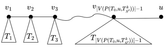
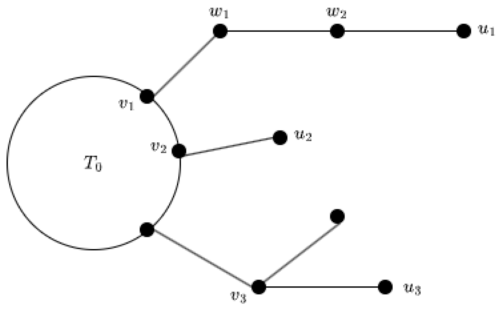
Recall that a path P is said to be a pendent path in a graph G if each internal vertices of P is also an internal vertex of G, while one endpoint of P is a leaf of G [15]. Here, we extends the concept of pendent path and named it as quasi-pendent path, which is defined as follows. Let $T^{\prime }$ be a sub-tree of T such that $V\left(T_0\right)\subseteq V\left(T^{\prime }\right)$ and $\mathit{\ell }\left(T^{\prime }\right)\setminus V\left(T_0\right)\ne \varnothing$. The quasi-pendent path $P(T_0,u,T^{\prime })$ of the leaf $u\in \mathit{\ell }\left(T^{\prime }\right)\setminus V\left(T_0\right)$ in $T^{\prime }$ is a non-trivial path such that: (1) u is one endpoint of $P(T_0,u,T^{\prime })$; (2) If $P(T_0,u,T^{\prime })$ contains internal vertices, then each internal vertex of $P(T_0,u,T^{\prime })$ is also an internal vertex of $T^{\prime }$ (with degree 2 in $T^{\prime }$) but does not belong to $V\left(T_0\right)$; (3) The other endpoint of $P(T_0,u,T^{\prime })$ is either in $V\left(T_0\right)$ or a branching vertex of $T^{\prime }$. Please see Figure 1 for an example of quasi-pendent paths.

Lemma 7.

For every fixed $k^{\prime }$-set R of a tree T and every sub-tree $T^{\prime }$ satisfying that $V\left(T_0\right)\subseteq V\left(T^{\prime }\right)$ and $\mathit{\ell }\left(T^{\prime }\right)\setminus V\left(T_0\right)\ne \varnothing$, the quasi-pendent path $P(T_0,u,T^{\prime })$ of a leaf $u\in \mathit{\ell }\left(T^{\prime }\right)\setminus V\left(T_0\right)$ always exists and is unique.

Proof. 

Let $v\in V\left(T_0\right)$ and $u\in \mathit{\ell }\left(T^{\prime }\right)\setminus V\left(T_0\right)$. Since $T^{\prime }$ is a tree, $P_{T^{\prime }}(u,v)$ is the unique path between u and v in $T^{\prime }$. Note that the path $P_{T^{\prime }}(u,v)$ always exists since T is a tree which is connected. Let $v^{\prime }$ be the nearest vertex to u among all vertices on $P_{T^{\prime }}(v,u)$ satisfying: (1) if $V\left(P_{T^{\prime }}(v^{\prime },u)\right)\setminus \{v^{\prime },u\}\ne \varnothing$, then $de{g}_{T^{\prime }}\left(w\right)=2$ and $w\notin V\left(T_0\right)$ for each vertex $w\in V\left(P_{T^{\prime }}(v^{\prime },u)\right)\setminus \{v^{\prime },u\}$; (2) either $de{g}_{T^{\prime }}\left(v^{\prime }\right)\ge 3$ or $v^{\prime }\in V\left(T_0\right)$.

Since $Neighbo{r}_T\left(u\right)\ne \varnothing$, the vertex $v^{\prime }$ could not be u. In addition, there could not be two distinct vertices on $P_{T^{\prime }}(u,v)$ such that both of them satisfies the above conditions. Otherwise, either one of them would not be the nearest one to u, or there would be a cycle in T. So the quasi-pendent path of a leaf in a tree is unique and always exists.    □

Lemma 8.

Let $R\subseteq V\left(T\right)$ be a fixed $k^{\prime }$-set in a tree T. Let v be the endpoint of $P(T_0,u,T_R^k)$ such that $v\ne u$. Let $(v,w)\in E\left(P(T_0,u,T_R^k)\right)$. Let F be the forest obtained by deleting the edge $(v,w)$ from T. Let $T_v$ and $T_w$ be the sub-trees in F, respectively, containing v and w. We have $R\cap V\left(T_w\right)=\varnothing$.

Proof. 

If $R\cap \left(V\left(T_w\right)\right)\ne \varnothing$, then let $x\in R\cap V\left(T_w\right)$. According to the definition of the quasi-pendent path, $R\cap \left(V(P(T_0,u,T_R^k)\setminus \left\{v\right\})\right)=\varnothing$. So $x\in (R\cap V\left(T_w\right))\setminus (V\left(P(T_0,u,T_R^k)\right)\setminus \left\{v\right\})$. Then, $P_{T_R^k}(v,x)$ must have common vertex with the path $P(T_0,u,T_R^k)$. So, a vertex in $V\left(P(T_0,u,T_R^k)\right)\setminus \left\{v\right\}$ must be a degree larger than two. This contradicts the fact that $P(T_0,u,T_R^k)$ is a quasi-pendent path.    □

2.2. Eccentricity of a Steiner $(k,k^{\prime })$-ecc R-Tree

Let H be a subgraph of a tree T, and $v\in V\left(T\right)$. The shortest path between v and H in T is denoted by $P_T(v,H)$. In $P_T(v,H)$, v is marked as $source\left(P_T(v,H)\right)$ while the other endpoint of $P_T(v,H)$ is marked as $dest\left(P_T(v,H)\right)$. The distance between v and H in T which is denoted by $di{s}_T(v,H)$ is the size of $P_T(v,H)$. The eccentricity of H in T is $ecc(H,T)$ = ${max}_{v\in V\left(T\right)}\left(di{s}_T(v,H)\right)$.

Lemma 9.

Let H be a subgraph of a tree T, and $v\in V\left(T\right)$. Let $v^{\prime }=dest\left(P_T(v,H)\right)$. Then, $v^{\prime }\in V\left(H\right)$ and $(V\left(P_T(v,H)\right)\setminus \left\{v^{\prime }\right\})\cap V\left(H\right)=\varnothing$.

Proof. 

If $v\in V\left(H\right)$, then according to the definition, $v=v^{\prime }$. So, obviously, $v^{\prime }\in V\left(H\right)$ and $V\left(P_G(v,H)\right)\setminus \left\{v^{\prime }\right\}\cap V\left(H\right)=\varnothing$.

If $v\notin V\left(H\right)$, then $v\ne v^{\prime }$. Suppose on the contrary that $(V\left(P_T(v,H)\right)\setminus \left\{v^{\prime }\right\})\cap V\left(H\right)\ne \varnothing$. There is a vertex $u\in V\left(P_T(v,H)\right)$ such that $u\ne v^{\prime }$ and $u\in V\left(H\right)$. Let $P^{\prime }$ be the sub-path between v and u. Due to the reason that $P_T(v,H)$ is the shortest path between v and $v^{\prime }$, its sub-path $P^{\prime }$ is a shortest path between v and u. In addition, the length of $P^{\prime }$ is strictly smaller than that of $P_T(v,H)$ since $v^{\prime }\ne u$. This contradicts the fact that $P_T(v,H)$ is a shortest path between v and H, because u is a vertex in $V\left(H\right)$ and $P_1$ is smaller than $P_T(v,H)$.    □

Lemma 10.

Let $T_1$ and $T_2$ be two distinct sub-trees of a tree T such that $V\left(T_1\right)\cap V\left(T_2\right)\ne \varnothing$. If $dest\left(P_T(v,T_2)\right)\notin V\left(T_1\right)$, then $V\left(P_T(v,T_2)\right)\cap V\left(T_1\right)=\varnothing$.

Proof. 

Let $P=P_T(v,T_2)$. Suppose on the contrary that $V\left(P\right)\cap V\left(T_1\right)\ne \varnothing$. Let $u\in V\left(P\right)\cap V\left(T_1\right)$. Let w be the nearest vertex to $dest\left(P\right)$ among all vertices in $V\left(T_1\right)\cap V\left(T_2\right)$, i.e., $w=dest\left(P_T(dest\left(P\right),V\left(T_1\right)\cap V\left(T_2\right))\right)$.

If $w=u$, then the path P would be the form $v\sim w\sim dest\left(P\right)$ because the path from $source\left(P\right)$ to $dest\left(P\right)$ in tree T is unique. Thus, $V\left(P\right)\setminus \left\{dest\left(P\right)\right\}\cap V\left(T_2\right)\ne \varnothing$. By Lemma 9, this contradicts the fact that P is the shortest between v and $T_2$.

Now, let us consider the case that $w\ne u$. Then, then the path between u and $dest\left(P\right)$ does go through w. Since $T_1$ is a tree u and w are connected in $T_1$. To ensure the connectivity in $T_1$, the path between u and w is the form $u\sim dest\left(P\right)\sim w$, and must be in the tree $T_1$. Then, the path between w and $dest\left(P\right)$ is in $T_1$. This contradicts the fact that $dest\left(P\right)$ does not belong to $V\left(T_1\right)$.    □

Let H be a subtree in a tree T. If $v\in V\left(T\right)$ satisfies $di{s}_T(v,H)=ecc(H,T)$, then the path $P_T(v,H)$ is said to be an H-ecc path. In addition, v is said to be the head of the H-ecc path and is marked as $Head\left(P_T(v,H)\right)$, while the other endpoint $dest\left(P_T(v,H)\right)$ is said to be the tail of the H-ecc path and marked as $Tail\left(P_T(v,H)\right)$. Let $Far(H,T)\subseteq V\left(T\right)$ be the set of heads of all H-ecc paths. Every vertex in $Far(H,T)$ is said to be a farthest vertex away from H in T.

Lemma 11.

Let $T^{\prime }$ be a sub-tree of a tree T such that $\mathit{\ell }\left(T\right)\setminus V\left(T^{\prime }\right)\ne \varnothing$. Every vertex in $Far(T^{\prime },T)$ is a leaf of T.

Proof. 

Let $V_1=V\left(T\right)\setminus V\left(T^{\prime }\right)$. Then, $V_1\ne \varnothing$ because of $\mathit{\ell }\left(T\right)\setminus V\left(T^{\prime }\right)\ne \varnothing$. Let $w\in Far(T^{\prime },T)$ be the head of a $T^{\prime }$-ecc path, and $w^{\prime }$ be the tail of the $T^{\prime }$-ecc path. By Lemma 9, $w\in V_1$. If $de{g}_T\left(w\right)\ge 2$, then there must be a leaf $w^{″}$ such that the path $P_T(w,w^{″})$ has no common edges with the $T^{\prime }$-ecc path. Then, the path $P_T(w^{″},w^{\prime })$ is the shortest path between $w^{″}$ and $T^{\prime }$, since in a tree, there is a unique path $P_T(w^{″},w^{\prime })$. Moreover, $P_T(w^{″},w^{\prime })$ is strictly longer than the path $P_T(w,w^{\prime })$, which contradicts the fact that $P_T(w,w^{\prime })$ is a $T^{\prime }$-ecc path.    □

Lemma 12.

Let $R\subseteq V\left(T\right)$ be a fixed $k^{\prime }$-set in a tree T. Let $T_1$ and $T_2$, respectively, be two distinct Steiner $(k,k^{\prime })$-ecc R-trees. Let $P_1$ be a $T_1$-ecc path and $P_2$ be a $T_2$-ecc path. If $|\mathit{\ell }\left(T\right)\setminus R|>k-k^{\prime }$, then both $Tail\left(P_1\right)$ and $Tail\left(P_2\right)$ belong to the set $V\left(T_1\right)\cap V\left(T_2\right)$.

Proof. 

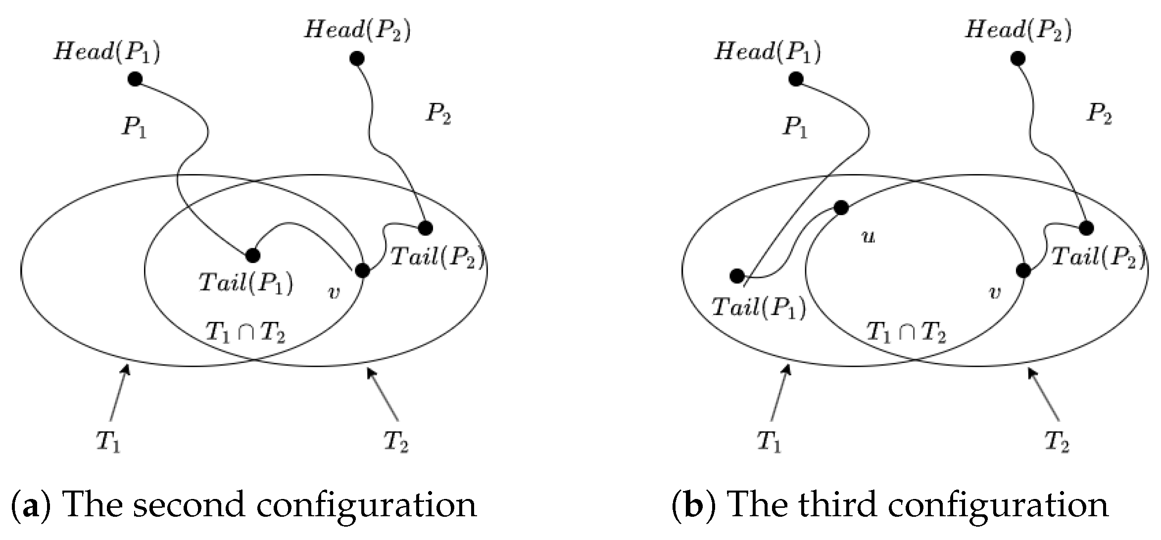
Since $R\ne \varnothing$, we have $V\left(T_1\right)\cap V\left(T_2\right)\ne \varnothing$. In other words, there are common vertices between $T_1$ and $T_2$. So there are three configurations for the positions of $Tail\left(P_1\right)$ and $Tail\left(P_2\right)$. The first one is that $Tail\left(P_1\right)$ and $Tail\left(P_2\right)$ both belong to the set $V\left(T_1\right)\cap V\left(T_2\right)$. The second configuration is that one of them is in $V\left(T_1\right)\cap V\left(T_2\right)$ and the other one is in $(V\left(T_1\right)\setminus V\left(T_2\right))\cup (V\left(T_2\right)\setminus V\left(T_1\right))$. The last one is that $Tail\left(P_1\right)\in V\left(T_1\right)\setminus V\left(T_2\right)$ and $Tail\left(P_2\right)\in V\left(T_2\right)\setminus V\left(T_1\right)$. In the following proof, we will, respectively, show that the second and third configurations could not occur.

Let us prove that the second configuration could not occur. By Lemma 9, $Tail\left(P_1\right)$ could not in $V\left(T_2\right)\setminus V\left(T_1\right)$, and $Tail\left(P_2\right)$ could not in $V\left(T_1\right)\setminus V\left(T_2\right)$. Without loss of generality, let $Tail\left(P_1\right)\in V\left(T_1\right)\cap V\left(T_2\right)$ and $Tail\left(P_2\right)\in V\left(T_2\right)\setminus V\left(T_1\right)$. We will derive a contradiction through the following statements.

Let $v\in V\left(T_1\right)\cap V\left(T_2\right)$ such that v is the nearest vertex to $Tail\left(P_2\right)$ among all vertices in $V\left(T_1\right)\cap V\left(T_2\right)$. See Figure 2a for this configuration. By Lemma 10, no vertex of $P_2$ is in $T_1$. By the assumption, $v\ne Tail\left(P_2\right)$. Because $P_1$ is a $T_1$-ecc path of $T_1$ and the path between v and $Head\left(P_2\right)$ is the shortest path between $Head\left(P_2\right)$ and $T_1$, the length of $P_1$ is no less than the length of the path between v and $Head\left(P_2\right)$ in T. Since $v\ne Tail\left(P_2\right)$, $P_1$ is longer than $P_2$.

According to the assumption, $Tail\left(P_1\right)\in V\left(T_1\right)\cap V\left(T_2\right)$ is also a vertex in $T_2$. Therefore, the contradiction is that $P_2$ is not a $T_2$-ecc path. So, the second configuration could not occur.

Finally, let us prove that the third configuration could also not occur. Suppose on the contrary that $Tail\left(P_1\right)\in V\left(T_1\right)\setminus V\left(T_2\right)$ and $Tail\left(P_2\right)\in V\left(T_2\right)\setminus V\left(T_1\right)$. Let $v\in V\left(T_1\right)\cap V\left(T_2\right)$ such that v is the nearest vertex to $Tail\left(P_2\right)$ among all vertices in $V\left(T_1\right)\cap V\left(T_2\right)$. Let $u\in V\left(T_1\right)\cap V\left(T_2\right)$ such that u is the nearest vertex to $Tail\left(P_1\right)$ among all vertices in $V\left(T_1\right)\cap V\left(T_2\right)$. By Lemma 10, $V\left(P_1\right)\cap V\left(T_2\right)=\varnothing$ and $V\left(P_2\right)\cap V\left(T_1\right)=\varnothing$ both hold true. See Figure 2b, for this configuration.

Without loss of generality, let the length of $P_1$ be no larger than that of $P_2$, i.e., $|E\left(P_1\right)|\le |E\left(P_2\right)|$. Since $v\ne Tail\left(P_2\right)$, then the path between v and $Head\left(P_2\right)$ is strictly longer than the path $P_1$. This contradicts the fact that the path between v and $Head\left(P_2\right)$ is the shortest path between $Head\left(P_2\right)$ and $T_1$ and $P_1$ is a $T_1$-ecc path. So the third configuration also could not occur.

All in all, $Tail\left(P_1\right)$ and $Tail\left(P_2\right)$ both belong to the set $V\left(T_1\right)\cap V\left(T_2\right)$.    □

Theorem 1.

Let $R\subseteq V\left(T\right)$ be a fixed $k^{\prime }$-set in a tree T. Let $T_1$ and $T_2$, respectively, be two distinct Steiner $(k,k^{\prime })$-ecc R-trees. We have $ecc(T_1,T)=ecc(T_2,T)$.

Proof. 

If $|\mathit{\ell }\left(T\right)\setminus R|\le k-k^{\prime }$, by Lemma 6, $T_1=T_2=T$. Otherwise, from Lemma 12, we know that the tail of $T_1$-ecc path and the tail of $T_2$-ecc path are both in the set $V\left(T_1\right)\cap V\left(T_2\right)$. In addition, by Lemma 1, the induced subtree $T_1[V\left(T_1\right)\cap V\left(T_2\right)]$ is the same as $T_2[V\left(T_1\right)\cap V\left(T_2\right)]$. Let $T_C=T_1[V\left(T_1\right)\cap V\left(T_2\right)]$. Then, the $T_1$-ecc path, as well as the $T_2$-ecc path is just the $T_c$-ecc path. Therefore, the length of $T_1$-ecc path is equal to that of $T_2$-ecc path.    □

3. The Structure of Optimal Solutions

This section studies the structure of optimal solutions on trees, which is a support for the $O\left(kn\right)$-time algorithm of Section 4. The structural properties are stated in Theorems 2 and 3. Given a vertex $k^{\prime }$-set $R\subseteq V\left(G\right)$ and an integer $k\ge k^{\prime }$, Theorem 2 indicates that each Steiner $(k,k^{\prime })$-ecc R-tree contains some Steiner $(k-1,k^{\prime })$-ecc R-tree. But, this does not mean that each any Steiner $(k-1,k’)$-ecc R-tree is contained by a Steiner $(k,k’$)-ecc R-tree. A trivial questions whether there is a Steiner $(k-1,k’$)-ecc R-tree not owned by any Steiner $(k,k’)$-ecc R-tree. Theorem 3 answers this question and says that each Steiner $(k-1,k^{\prime })$-ecc R-tree is contained by some Steiner $(k,k^{\prime })$-ecc R-tree. It is a little stronger.

Lemma 13.

Let $R\subseteq V\left(G\right)$ be a fixed $k^{\prime }$-set in a tree T such that $|\mathit{\ell }\left(T\right)\setminus R|>k-k^{\prime }>0$. Let u be a leaf in $\mathit{\ell }\left(T_R^k\right)\setminus \mathit{\ell }\left(T_R^{k-1}\right)$. If $E\left(P(T_0,u,T_R^k)\right)\cap E\left(T_R^{k-1}\right)\ne \varnothing$, then there exists $x\in \mathit{\ell }\left(T_R^{k-1}\right)$ and $v\in V\left(T_0\right)$ such that $V\left(P_T(v,x)\right)\setminus \left\{v\right\}\cap V\left(T_0\right)=\varnothing$ and $E\left(P(T_0,u,T_R^k)\right)\cap E\left(P_T(v,x)\right)\ne \varnothing$.

Proof. 

Since $P(T_0,u,T_R^k)$ has common edges with $T_R^{k-1}$, then there exist $x\in \mathit{\ell }\left(T_R^{k-1}\right)$ and $v\in V\left(T_R^{k-1}\right)\setminus \left\{x\right\}$ such that $E\left(P(T_0,u,T_R^k)\right)\cap E\left(P_T(v,x)\right)\ne \varnothing$. Given vertex $x\in \mathit{\ell }\left(T_R^{k-1}\right)$, let $V_x\subseteq V\left(T_R^{k-1}\right)\setminus \left\{x\right\}$ be the vertex set such that $E\left(P(T_0,u,T_R^k)\right)\cap E\left(P_T(v,x)\right)\ne \varnothing$ holds true for every vertex $v\in V_x$. Let $u^{\prime }$ be the endpoint of $P(T_0,u,T_R^k)$ such that $u^{\prime }\ne u$. By Lemma 2, let $u_1,u_2\in V\left(P(T_0,u,T_R^k)\right)\cap V\left(P_T(v,x)\right)$ such that the common portion of $P(T_0,u,T_R^k)$ and $P_T(v,x)$ is $P_T(u_1,u_2)$, where $v\in V_x$. Without loss of generality, let $u_1$ be farther to x than $u_2$. See Figure 3.

We claim that $V\left(P_T(u_1,x)\right)\setminus \left\{u_1\right\}\cap V\left(T_0\right)=\varnothing$. Since $P_T(u_1,u_2)$ is a sub-path of $P(T_0,u,T_R^k)$, then, by Lemma 8 and the definition of quasi-pendent path $V\left(P_T(u_1,u_2)\right)\setminus \left\{u_1\right\}\cap V\left(T_0\right)=\varnothing$. Now we prove that $V\left(P_T(u_2,x)\right)\cap V\left(T_0\right)=\varnothing$. Assume on the contrary that $V\left(P_T(u_2,x)\right)\cap V\left(T_0\right)\ne \varnothing$. Then, by Lemma 5, $T_R^k$ contains a path between $u_2$ and a vertex in $V\left(T_0\right)$. This implies that the degree of $u_2$ is at least three in $T_R^k$. Recall that $u_2$ is an internal vertex of $P(T_0,u,T_R^k)$. By definition, this is a contradiction.

Now, we prove that $V_x\cap V\left(T_0\right)\ne \varnothing$ and there is a vertex $v\in V_x\cap V\left(T_0\right)$ such that $V\left(P_T(v,x)\right)\setminus \left\{v\right\}\cap V\left(T_0\right)=\varnothing$. Because $V\left(P_T(u_1,x)\right)\setminus \left\{u_1\right\}\cap V\left(T_0\right)=\varnothing$, we just need to prove that $V_x\cap V\left(T_0\right)\ne \varnothing$ and there is a vertex $v\in V_x\cap V\left(T_0\right)$ such that $V\left(P_T(v,u_1)\right)\setminus \left\{v\right\}\cap V\left(T_0\right)=\varnothing$. We prove this proposition by discussing whether $u^{\prime }$ is in $V\left(T_0\right)$ or not.

If $u^{\prime }\in V\left(T_0\right)$, then the path $P_T(u^{\prime },x)$ satisfying that $E\left(P(T_0,u,T_R^k)\right)\cap E\left(P_T(u^{\prime },x)\right)\ne \varnothing$. Thus, $u^{\prime }\in V_x\cap V\left(T_0\right)$ and $V\left(P_T(u^{\prime },x)\right)\setminus \left\{u^{\prime }\right\}\cap V\left(T_0\right)=\varnothing$.

Now, let us consider the case that $u^{\prime }\notin V\left(T_0\right)$. By Lemma 5, since the path $P(T_0,u,T_R^k)$ and $T_0$ are connected, there is a vertex $w\in V\left(P(T_0,u,T_R^k)\right)$ and a vertex $w^{\prime }\in V\left(T_0\right)$ such that w and $w^{\prime }$ is connected through a path in $T_R^k$ and $V\left(P_{T_R^k}(w^{\prime },w)\right)\setminus \left\{w^{\prime }\right\}\cap V\left(T_0\right)=\varnothing$, since $T_0$ is a sub-tree of $T_R^k$.

We claim that $w=u^{\prime }$. Otherwise, let $w\in V\left(P(T_0,u,T_R^k)\right)\setminus \left\{u^{\prime }\right\}$ such that there is a path between w and $w^{\prime }$ in $T_R^k$. Then, the degree of w in $T_R^k$ is at least three since the path $P_T(w,u)$ is also a part of $T_R^k$. This contradicts the fact that $P_{T_R^k}(u^{\prime },u)$ is a quasi-pendent path.

So w must be equal to $u^{\prime }$. Then, $w^{\prime }\in V_x\cap V\left(T_0\right)$ such that $V\left(P_T(w^{\prime },x)\right)\setminus \left\{w^{\prime }\right\}\cap V\left(T_0\right)=\varnothing$. Therefore, the lemma holds.    □

Lemma 14.

Given a leaf $u\in \mathit{\ell }\left(T\right)$, if there exist two distinct leaves $u_1,u_2\in \mathit{\ell }\left(T_R^k\right)$ and a vertex $v\in V\left(T_0\right)$ such that $V(\left(P_T(v,u)\right)\setminus \left\{v\right\})\cap V\left(T_0\right)=\varnothing$, $E\left(P_T(v,u)\right)\cap E\left(P(T_0,u_1,T_R^k)\right)\ne \varnothing$ and $E\left(P_T(v,u)\right)\cap E\left(P(T_0,u_2,T_R^k)\right)\ne \varnothing$, then neither the other endpoint of $P(T_0,u_1,T_R^k)$ nor the other endpoint of $P(T_0,u_2,T_R^k)$ is in the set $V\left(T\right)\setminus V\left(P_T(v,u)\right)$.

Proof. 

Let $u_1^{\prime }$ be the other endpoint of $P(T_0,u_1,T_R^k)$, and $u_2^{\prime }$ be the other endpoint of $P(T_0,u_2,T_R^k)$. By Lemma 2, the common part which is shared by $P(T_0,u_1,T_R^k)$ and $P_T(v,u)$ is a single path. In addition, the common part which is shared by $P(T_0,u_2,T_R^k)$ and $P_T(v,u)$ is also a single path. Suppose on the contrary that $u_1^{\prime }$ is not on the path $P_T(v,u)$. Then, $u_1^{\prime }\ne v$. In addition, v is neither on the path $P_T(u_1^{\prime },u)$ nor on the path $P_T(u_1^{\prime },u_1)$ because $v\in V\left(T_0\right)$ and every vertex in $V\left(P(T_0,u_1,T_R^k)\right)\setminus \left\{u_1^{\prime }\right\}$ does not belong to $V\left(T_0\right)$. In the tree T, the two paths $P(T_0,u_1,T_R^k)$ and $P(T_0,u_2,T_R^k)$ are connected by some edges of $P_T(v,u)$, because they both share edges with $P_T(v,u)$.

Because the vertices excluding the endpoints of $P(T_0,u_1,T_R^k)$ and $P(T_0,u_2,T_R^k)$ are all internal vertices in $T_R^k$, there is no edge of $P_T(v,u)$ connecting $P(T_0,u_1,T_R^k)$ and $P(T_0,u_2,T_R^k)$ in $T_R^k$. So, in the tree $T_R^k$, there is a sub-tree $T^{\prime }$ connecting the three vertices v, $u_1^{\prime }$ and $u_2^{\prime }$ such that $E\left(T^{\prime }\right)\setminus E\left(P_T(v,u)\right)\ne \varnothing$, since $u_1^{\prime }\ne v$. This implies that there is a cycle in the tree T. It is in the same way to prove that $u_2^{\prime }$ could not be in the set $V\left(T\right)\setminus V\left(P_T(v,u)\right)$. So, the lemma holds.    □

Lemma 15.

Given a leaf $u\in \mathit{\ell }\left(T\right)$, if there exist two distinct leaves $u_1,u_2\in \mathit{\ell }\left(T_R^k\right)$ and a vertex $v\in V\left(T_0\right)$ such that $V(\left(P_T(v,u)\right)\setminus \left\{v\right\})\cap V\left(T_0\right)=\varnothing$, $E\left(P_T(v,u)\right)\cap E\left(P(T_0,u_1,T_R^k)\right)\ne \varnothing$ and $E\left(P_T(v,u)\right)\cap E\left(P(T_0,u_2,T_R^k)\right)\ne \varnothing$, then it is impossible that $u\ne u_1$ and $u\ne u_2$ occur simultaneously.

Proof. 

Let $P_0=P_T(v,u)$, $u_1^{\prime }$ be the other endpoint of $P(T_0,u_1,T_R^k)$ and $u_2^{\prime }$ be the other endpoint of $P(T_0,u_2,T_R^k)$. By Lemma 2, let $P_1$ be the common part of $P_0$ and $P(T_0,u_1,T_R^k)$. Let $P_2$ be the common part of $P_0$ and $P(T_0,u_2,T_R^k)$.

By Lemma 14, $u_1^{\prime }\notin V\left(T\right)\setminus V\left(P_0\right)$ and $u_2^{\prime }\notin V\left(T\right)\setminus V\left(P_0\right)$. It might only be possible that $u_1^{\prime }\in V\left(P_0\right)$ and $u_2^{\prime }\in V\left(P_0\right)$. Since there is no cycle in tree T, as well as in $T_R^k$, $P_1$ and $P_2$ are connected in the tree $T_R^k$ by only the edges of $P_0$. In addition, $P(T_0,u_1,T_R^k)$ and $P(T_0,u_2,T_R^k)$ are connected in the tree $T_R^k$ by only the edges of $P_0$. Suppose on the contrary that $u\ne u_1$ and $u\ne u_2$ occur simultaneously. Then, one endpoint of $P_1$ and $P_2$, excluding $u_1^{\prime }$ and $u_2^{\prime }$, would have degree three. This is a contradiction because $P(T_0,u_1,T_R^k)$ and $P(T_0,u_2,T_R^k)$ are both quasi-pendent paths in $T_R^k$.    □

Lemma 16.

Let $R\subseteq V\left(G\right)$ be a $k^{\prime }$-set in a tree T. If $|\mathit{\ell }\left(T\right)\setminus R|>k-k^{\prime }>0$, then there is a leaf $u\in \mathit{\ell }\left(T_R^k\right)\setminus \mathit{\ell }\left(T_R^{k-1}\right)$ such that $E\left(P(T_0,u,T_R^k)\right)\cap E\left(T_R^{k-1}\right)=\varnothing$.

Proof. 

Suppose on the contrary that for every leaf $u\in \mathit{\ell }\left(T_R^k\right)\setminus \mathit{\ell }\left(T_R^{k-1}\right)$ the quasi-pendent path $P(T_0,u,T_R^k)$ has common edges with $T_R^{k-1}$. Then, by Lemma 13, for every leaf $u\in \mathit{\ell }\left(T_R^k\right)\setminus \mathit{\ell }\left(T_R^{k-1}\right)$ there exist $u_1\in \mathit{\ell }\left(T_R^{k-1}\right)$ and $v\in V\left(T_0\right)$ such that $V\left(P_T(v,u)\right)\setminus \left\{v\right\}\cap V\left(T_0\right)=\varnothing$ and $E\left(P(T_0,u,T_R^k)\right)\cap E\left(P_T(v,u_1)\right)\ne \varnothing$. In addition, by Lemma 15, for a leaf $u\in \mathit{\ell }\left(T_R^{k-1}\right)$, two distinct leaves $u_1,u_2\in \mathit{\ell }\left(T_R^k\right)\setminus \mathit{\ell }\left(T_R^{k-1}\right)$ and a vertex $v\in V\left(T_0\right)$ do not exist, such that $V\left(P_T(v,u)\right)\setminus \left\{v\right\}\cap V\left(T_0\right)=\varnothing$, $E\left(P(T_0,u_1,T_R^k)\right)\cap E\left(P_T(v,u)\right)\ne \varnothing$ and $E\left(P(T_0,u_2,T_R^k)\right)\cap E\left(P_T(v,u)\right)\ne \varnothing$ are all true. This implies that the number of leaves in $T_R^{k-1}$ is no less than that in $T_R^k$. This contradicts Corollary 1.    □

Lemma 17.

Let $R\subseteq V\left(G\right)$ be a $k^{\prime }$-set in a tree T such that $|\mathit{\ell }\left(T\right)\setminus R|>k-k^{\prime }>0$. Let $P(T_0,u,T_R^k)$ be a quasi-pendent path of a leaf $u\in \mathit{\ell }\left(T_R^k\right)$ such that $E\left(T_R^{k-1}\right)\cap E\left(P(T_0,u,T_R^k)\right)=\varnothing$. Let S be the $(k-1)$-set corresponding to $T_R^{k-1}$, and $T^{\prime }=Stei(S\cup \left\{u\right\})$. We have $E\left(P(T_0,u,T_R^k)\right)\subseteq E\left(P(T_0,u,T^{\prime })\right)$.

Proof. 

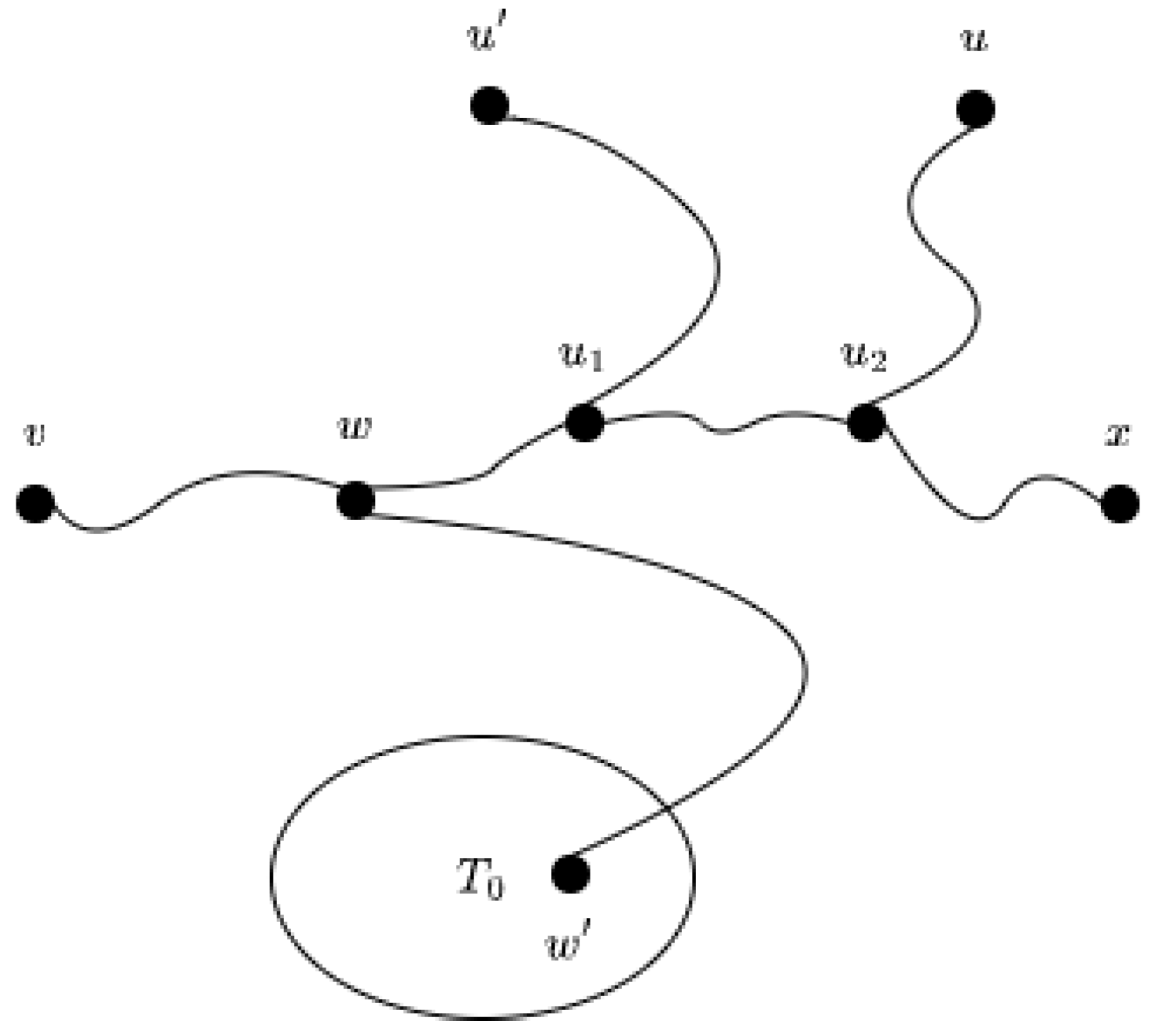
Let $P(T_0,u,T_R^k)=$$v_1,\dots ,v_{\left|V\right(P(T_0,u,T_R^k)\left)\right|-1},u$, where $v_1$ is the other endpoint such that $u\ne v_1$. If all edges in $P(T_0,u,T_R^k)$ were deleted from $T_R^k$, we would achieve a series of sub-trees which, respectively, contain $v_1,\dots ,v_{\left|V\right(P(T_0,u,T_R^k)\left)\right|-1}$ and u. Let $T_i:1\le i\le \left|V\left(P(T_0,u,T_R^k)\right)\right|-1$ be the sub-tree containing the vertex $v_i$. Please see Figure 4 for this configuration.

Because $P(T_0,u,T_R^k)$ has no common edge with $T_R^{k-1}$, we have $S\cap (V\left(T\right)\setminus V\left(T_1\right))=\varnothing$. Otherwise, suppose on the contrary that there is a vertex $w\in V\left(T\right)\setminus V\left(T_1\right)$ such that w is also in S. By Lemma 8, we have $R\cap (V\left(T\right)\setminus V\left(T_1\right))=\varnothing$. So there is a vertex $w^{\prime }\in R$ such that $w\ne w^{\prime }$ and there is a path between w and $w^{\prime }$ in $T_R^{k-1}$. Moreover, the path between w and $w^{\prime }$ is unique in the T. So the path between w and $w^{\prime }$ in $T_R^{k-1}$ must contain the edge $(v_1,v_2)$. This leads to a contradiction that $P(T_0,u,T_R^k)$ has a common edge with $T_R^{k-1}$.

Thus, the minimum Steiner tree $T^{\prime }$ on the set $S\cup \left\{u\right\}$ contains the entire path $P(T_0,u,T_R^k)$, but does not contain any edge in $E\left(T\right)\setminus (E\left(T_1\right)\cup E\left(P(T_0,u,T_R^k)\right))$ any more. Therefore, the quasi-pendent path $P(T_0,u,T^{\prime })$ of u in $T^{\prime }$ must contain the entire path $P(T_0,u,T_R^k)$.    □

Let $T_1$ and $T_2$, respectively, be two trees. The union of $T_1$ and $T_2$ is a new tree T such that $V\left(T\right)=V\left(T_1\right)\cup V\left(T_2\right)$ and $E\left(T\right)=E\left(T_1\right)\cup E\left(T_2\right)$.

Theorem 2.

Let $R\subseteq V\left(G\right)$ be a $k^{\prime }$-set in a tree T. If $|\mathit{\ell }\left(T\right)\setminus R|>k-k^{\prime }>0$, then given a Steiner $(k,k^{\prime })$-ecc R-tree $T_R^k$, there is a Steiner $((k-1),k^{\prime })$-ecc R-tree which is contained by $T_R^k$.

Proof. 

Suppose on the contrary that a Steiner $(k,k^{\prime })$-ecc R-tree $T_R^k$ does not contain any Steiner $((k-1),k^{\prime })$-ecc R-tree. Let $T_R^{k-1}$ be a Steiner $((k-1),k^{\prime })$-ecc R-tree. Then, by the assumption, $T_R^k$ does not contain the entire tree $T_R^{k-1}$.

By Lemma 16, there is a leaf $u\in \mathit{\ell }\left(T_R^k\right)\setminus V\left(T_R^{k-1}\right)$ such that the quasi-pendent path $P(T_0,u,T_R^k)$ has no common edge with $T_R^{k-1}$. Let $u^{\prime }$ be the other endpoint (which is different from u) of the path $P(T_0,u,T_R^k)$.

Let $S_1=S_R^k\setminus \left\{u\right\}$, where $S_R^k$ is the Steiner $(k,k^{\prime })$-ecc R-set corresponding to $T_R^k$. The tree $T_1=T_R^k[V\left(T_R^k\right)\setminus (V\left(P(T_0,u,T_R^k)\right)\setminus \left\{u^{\prime }\right\})]$ is the minimum Steiner tree on the $(k-1)$-set $S_1$. Because if $T_1$ is not a minimum Steiner tree on $S_1$, then the union of a smaller Steiner tree on $S_1$ (than $T_1$) and the path $P(T_0,u,T_R^k)$ could span all vertices in the set $S_R^k$, which contradicts the fact that $T_R^k$ is a minimum Steiner tree.

By that assumption, $T_1$ is strictly smaller than $T_R^{k-1}$. In other words, $|E\left(T_1\right)|<|E\left(T_R^{k-1}\right)|$. Moreover, according the construction, the union of $T_1$ and $P(T_0,u,T_R^k)$ is the entire tree $T_R^k$, i.e., $\left|E\right(T_1\left)\right|$ + $\left|E\right(P(T_0,u,T_R^k)\left)\right|$ = $\left|E\right(T_R^k\left)\right|$.

Now, let us turn to $T_R^{k-1}$. Let $S_R^{k-1}$ be the Steiner $((k-1),k^{\prime })$-ecc R-set corresponding to $T_R^{k-1}$. Let $S_2=S_R^{k-1}\cup \left\{u\right\}$. In the following proof, we are going to show that the minimum Steiner tree on the set $S_2$ is strictly larger than $T_R^k$. This contradicts the fact that $T_R^k$ is the maximum over all minimum Steiner trees on k-sets containing R.

Let $T_2$ be the minimum Steiner tree on the set $S_2$. By Lemma 17, the path $P(T_0,u,T_R^k)$ is a sub-path of $P(T_0,u,T_2)$. So, we have $\left|E\right(T_2\left)\right|$ ≥ $\left|E\right(T_R^{k-1}\left)\right|$ + $\left|E\right(P(T_0,u,T_R^k)\left)\right|$>$\left|E\right(T_1\left)\right|$ + $\left|E\right(P(T_0,u,T_R^k)\left)\right|$ = $\left|E\right(T_R^k\left)\right|$. Therefore, $T_2$ is strictly larger than $T_R^k$. This brings us to the contradiction.    □

Corollary 2.

Let $R\subseteq V\left(G\right)$ be a $k^{\prime }$-set in a tree T such that $|\mathit{\ell }\left(T\right)\setminus R|>k-k^{\prime }>0$. Let $T_R^{k-1}$ be a Steiner $(k-1,k^{\prime })$-ecc R-tree that is contained by a known Steiner $(k,k^{\prime })$-ecc R-tree $T_R^k$. There is a $T_R^{k-1}$-ecc path P such that the union of $T_R^{k-1}$ and P is the tree $T_R^k$. In addition, $\left|E\right(T_R^k\left)\right|=$ $\left|E\right(P\left)\right|$ + $\left|E\right(T_R^{k-1}\left)\right|$.

Proof. 

Let $T^{\ast }$ be a $T_R^k$ and $T_1$ be a $T_R^{k-1}$ such that $T_1$ is contained by $T^{\ast }$. Let $S^{\ast }$ and $S_1$ be the Steiner $(k,k^{\prime })$-ecc R-set and Steiner $((k-1),k^{\prime })$-ecc R-set, respectively, corresponding to $T^{\ast }$ and $T_1$.

Since $|\mathit{\ell }\left(T\right)\setminus R|>k-k^{\prime }>0$, by Lemma 6, $S^{\ast }\setminus R$ has exactly one more vertex than $S_1\setminus R$. Again, by Lemma 6, the extra vertex in the set $S^{\ast }\setminus R$ compared to the set $S_1\setminus R$ is a leaf of T. So the extra vertex is one of those vertices in $Far(T_R^{k-1},T)$. Thus, the union of $T_R^{k-1}$ and one of $T_R^{k-1}$-ecc paths is $T^{\ast }$. And the summation of the sizes of them is equal to the size of $T^{\ast }$.    □

Theorem 3.

Let $R\subseteq V\left(G\right)$ be a $k^{\prime }$-set in a tree T. If $|\mathit{\ell }\left(T\right)\setminus R|>k-k^{\prime }>0$, then given a $T_R^{k-1}$, there is a $T_R^k$ such that $T_R^k$ contains this $T_R^{k-1}$.

Proof. 

Let $T_1$ be the given $T_R^{k-1}$. Suppose on the contrary that there is no $T_R^k$ such that $T_R^k$ contains $T_1$. Let $T^{\ast }$ be a $T_R^k$. By Theorem 2, let $T_2$ be the $T_R^{k-1}$ which is contained by $T^{\ast }$.

According to the assumption, $T_1$ and $T_2$ are distinct. By Theorem 1, we have $ecc(T_1,T)=ecc(T_2,T)$. By Corollary 2, the union of $T_2$ and one of its $T_2$-ecc paths is just the tree $T^{\ast }$. So we have $|E\left(T^{\ast }\right)|=|E\left(T_2\right)|+ec{c}_T\left(T_2\right)$.

Let us turn to the tree $T_1$. Let P be an $T_1$-ecc path and w be the head of P, i.e., $w\in Far(T_1,T)$. By Lemma 11, w is a leaf of T. Let $S_1$ be the Steiner $(k,k^{\prime })$-ecc R-set corresponding to $T_1$. Then, $S=S_1\cup \left\{w\right\}$ is a k-set. The size of $Stei\left(S\right)$ is:

$$\left|E\left(Stei(S,G)\right)\right|=|E\left(T_1\right)|+|E\left(P\right)|=|E\left(T_1\right)|+ecc(T_1,T)=\left|E\left(T_1\right)\right|+ecc(T_2,T).$$

According to the assumption that $T_1$ is not contained by any $T_R^k$, then $Stei\left(S\right)$ is not a Steiner $(k,k^{\prime })$-ecc R-tree. So, $|E\left(T^{\ast }\right)|>|E\left(Stei\left(S\right)\right)|$. Then, we have $|E\left(T_2\right)|>|E\left(T_1\right)|$, which contradicts the fact that they are both Steiner $((k-1),k^{\prime })$-ecc R-trees. Therefore, the theorem holds.    □

Corollary 3.

Let $R\subseteq V\left(G\right)$ be a $k^{\prime }$-set in a tree T. If $|\mathit{\ell }\left(T\right)\setminus R|>k-k^{\prime }>0$, then given a Steiner $((k-1),k^{\prime })$-ecc R-tree $T_1$, the union of $T_1$ and P is a Steiner $(k,k^{\prime })$-ecc R-tree of R, where P is one of its $T_1$-ecc paths. In addition, the Steiner $(k,k^{\prime })$-eccentricity of R is $|E\left(T_1\right)|+|E\left(P\right)|$.

Proof. 

By Theorem 3, let $T^{\ast }$ be a $T_R^k$ such that $T^{\ast }$ contains $T_1$. By Corollary 2, there is a $T_1$-ecc path P such that the union of P and $T_1$ is $T^{\ast }$. And, the size of $T^{\ast }$ is equal to $\left|E\left(P\right)\right|+|E\left(T_1\right)|$.    □

4. The Algorithm

Let R be a given fixed $k^{\prime }$-set in a tree T. Let k be an integer such that $k\ge k^{\prime }$. If $|\mathit{\ell }\left(T\right)\setminus R|\le k-k^{\prime }$, by Lemma 6, the whole tree T is the optimal solution corresponding to Steiner $(k,k^{\prime })$-eccentricity of a given $k^{\prime }$-set. Now, we focus on the case that $|\mathit{\ell }\left(T\right)\setminus R|>k-k^{\prime }$.

According to Lemma 5, in order to compute the Steiner $(k,k^{\prime })$-eccentricity of R in a tree T, firstly we find the minimum Steiner tree on the set R, and then search for the remaining portion of a Steiner $(k,k^{\prime })$-ecc R-tree. This is the logical framework of our approach. This section presents an algorithm to realize this framework, in which the algorithm can not only find a minimum Steiner tree of a given set in $O\left(kn\right)$-time, but can also find the remaining portion of an optimal solution in $O\left(kn\right)$-time.

Given a vertex set $S\subseteq V\left(T\right)$ of a tree T, Algorithm 1 is to find $Stei\left(S\right)$ in the tree T. $Stei\left(S\right)$ is represented by black-colored vertices in the algorithm. Initially, the vertices in S are all colored black, while the vertices out of S are all colored white, since S must be in the tree $Stei\left(S\right)$. The next task is to find Steiner vertices so as to connect all vertices of S with a minimum number of edges. The algorithm runs a breadth-first search (BFS) procedure [16] beginning with an arbitrary source vertex in S. Whenever the search discovers an unvisited vertex v in the course of scanning an already discovered vertex u, the vertex v is marked as “visited”. We say that u is the predecessor or parent of v. The parent of vertices is stored in an array $pre(\ast )$ in Algorithm 1. By Lemma 4, whenever it meets a black vertex, all the vertices which are on the path from the source vertex to this newly discovered black vertex are colored black. Meanwhile, the parents of all these newly colored black vertex are marked as ⌀. This procedure is realized in Steps 15–17 in the Algorithm 1. At the end of the algorithm, every vertex in $Stei\left(S\right)$ is colored black, while those vertices out of $Stei\left(S\right)$ are all colored white.

Algorithm 1: Steiner-Tree(S, T)
	Input: A tree T and a vertex set $S\subseteq V\left(T\right)$
	Output: The minimum Steiner tree of S in T.
1	foreach $u\in V\left(T\right)$ do $color\left(u\right)$ ← white; $pre\left(u\right)$ ← ⌀; $visit\left(u\right)\leftarrow ⌀$;
2	foreach $u\in S$ do $color\left(u\right)$ ← black;
3	s ← Pick a vertex from S;									// The source for BFS
4	Q ←∅;									// Initialize an empty queue  Q
5	ENQUEUE(Q, s);
6	while $Q\ne \varnothing$ do
7			u ←$DEQUEUE\left(Q\right)$;
8			$visit\left(u\right)\leftarrow 1$;
9			foreach $w\in Neighbo{r}_T\left(u\right)$ do
10					if $color\left(w\right)==$ white and $visit\left(w\right)=⌀$ then
11							$pre\left(w\right)$ ←u;
12							$ENQUEUE(Q,w)$;
13					else if $color\left(w\right)==$ black and $visit\left(w\right)=⌀$ then
14							x ←u;
15							while $x\ne ⌀$ do			// By Lemma 4
16								$color\left(x\right)$ ← black; $y\leftarrow pre\left(x\right)$; $pre\left(x\right)\leftarrow ⌀$; $x\leftarrow y$;
17							end
18							$pre\left(w\right)$ ← ⌀;
19							$ENQUEUE(Q,w)$;
20			end
21	end
22	return The two arrays: $color(\ast )$ and $pre(\ast )$.

Now let us turn to the approach of computing Steiner $(k,k^{\prime })$-eccentricity. If $k=k^{\prime }$, then the Steiner $(k,k^{\prime })$-eccentricity of a fixed $k^{\prime }$-set R is the size of $Stei\left(R\right)$ in a tree T. The optimal solution can be earned directly from Algorithm 1. If $k>k^{\prime }$, by Corollary 3, our idea to find a Steiner $(k,k^{\prime })$-ecc R-tree basically needs the three following stages. Firstly, obtain a Steiner $((k-1),k^{\prime })$-ecc R-tree which is noted as $T_1$. Next, choose the maximum distance between $T_1$ and every leaf in $\mathit{\ell }\left(T\right)$. Finally, merge the shortest path which is between $T_1$ and the leaf into $T_1$. If $k-1>k^{\prime }$, then it is in the same way to earn $T_1$. Otherwise, $T_1$ can be earned by Algorithm 1. The whole process for computing Steiner $(k,k^{\prime })$-eccentricity of a given $k^{\prime }$-set in a tree is summarized in Algorithm 2. Its details are going to be stated in the following.

Given a vertex set $R\subseteq V\left(T\right)$ of a tree T, by Lemma 5, the set of vertices in $Stei\left(R\right)$ is naturally included in it. Algorithm 2 starts with the $Stei\left(R\right)$ in Step 1. The tree $Stei\left(R\right)$ is marked with black-colored vertices which are stored in the array $color(\ast )$. Subsequently, the algorithm calculates the distance between $Stei\left(R\right)$ and each leaf of T in Step 2. Finally, the Algorithm 2 goes through $k-k^{\prime }$ rounds of iteration in a while-loop, in which at each iteration it merges a farthest leaf with its corresponding shortest path into a partial solution.

Algorithm 3 calculate the distance between each vertex and the (already-discovered) partial solution. Note that every vertex in the partial solution has been colored black. If a vertex is in the partial solution, then the distance is zero. So the $dis(\ast )$ for each black vertex is zero. The algorithm is a BFS procedure beginning with a black vertex. Once a white vertex u occurs in the course of scanning an already discovered vertex v, then $dis\left(u\right)=dis\left(v\right)+1$. Recall that by Lemma 4 those vertices with a white vertex as an ancestor is white. Therefore, at the end of Algorithm 3, the array $dis(\ast )$ stores the distances between each vertex and the black-colored partial solution.

Algorithm 2: Steiner-ECC(R, k, T)
	Input: A tree T, a vertex set $R\subseteq V\left(T\right)$ and an integer $k\ge \left|R\right|$
	Output: Steiner $(k,k^{\prime })$-eccentricity of R.
1	$color$, $pre$ ← Steiner-Tree(R, T);			// Algorithm 1
2	$dis$ ← Get-dis(T, $color$, $pre$);			// Algorithm 3
3	i ← 1;
4	while $i\le (k-|R\left|\right)$ do			// By Corollary 3
5		v ← Find the maximum $dis(\ast )$ among all leaves in $\mathit{\ell }\left(T\right)$;
6		P ← ∅;		// An initial empty set P representing a path
7		P ← $P\cup \left\{v\right\}$;
8		while $pre\left(v\right)\ne ⌀$ do P ←$P\cup \left\{pre\right(v\left)\right\}$; $v\leftarrow pre\left(v\right)$;
9		foreach $u\in P$ do $color\left(u\right)$ ← black; $dis\left(u\right)\leftarrow 0$; $pre\left(u\right)\leftarrow ⌀$;
10		Update(P, $dis$, T);		// Algorithm 4
11	end
12	return The size of the subtree induced by the set of black vertices.

Algorithm 3: Get-dis(T, $color$, $pre$)
	Input: A tree T, two arrays $color(\ast )$ and $pre(\ast )$
	Output: The distance between every vertex and a subtree which is colored black
1	foreach $u\in V\left(T\right)$ do $visit\left(u\right)\leftarrow ⌀$;
2	s ← Pick a black vertex;							// The source for BFS.
3	$dis\left(s\right)$ ← 0;
4	Q ←∅;							// Initialize an empty queue  Q
5	$ENQUEUE(Q,s)$;
6	while $Q\ne \varnothing$ do
7			u ←$DEQUEUE\left(Q\right)$;
8			$visit\left(u\right)\leftarrow 1$;
9			foreach $w\in Neighbo{r}_T\left(u\right)$ do
10					if $color\left(w\right)==$ white and $visit\left(w\right)=⌀$ then
11						$dis\left(w\right)$ ←$dis\left(u\right)+1$
12						$ENQUEUE(Q,w)$;
13					else if $color\left(w\right)==$ black and $visit\left(w\right)=⌀$ then
14						$dis\left(w\right)$ ← 0;
15						$ENQUEUE(Q,w)$;
16			end
17	end
18	return The array $dis(\ast )$.

Once a leaf and its corresponding shortest path are merged into a partial solution, the array $dis(\ast )$ should be updated because the distances between the remaining leaves and the newly constructed partial solution would become smaller. The updating procedure is listed in Algorithm 4. Recall that only the distances of those vertices with ancestors on this merged shortest path might be decreased. So, Step 10 only considers those sub-trees hanging at the merged path. Algorithm 4 assigns 0 to $dis(\ast )$ for each vertex on the merged path, and runs a BFS procedure starting with each internal vertex of the merged path. Black vertices and those vertices on the merged path will not be traversed in this procedure.

Theorem 4.

There is an $O\left(kn\right)$-time algorithm to compute Steiner $(k,k^{\prime })$-eccentricity of a given fixed $k^{\prime }$-set $R\subseteq V\left(T\right)$ in a tree T, where n is the order of T.

Proof. 

By Lemma 6, if $|\mathit{\ell }\left(T\right)\setminus R|\le k-k^{\prime }$, the whole tree T is an optimal solution corresponding to Steiner $(k,k^{\prime })$-eccentricity of R. So it takes $O\left(n\right)$-time to earn Steiner $(k,k^{\prime })$-eccentricity.

If $|\mathit{\ell }\left(T\right)\setminus R|>k-k^{\prime }$, then the Algorithm 2 can be adopted to compute Steiner $(k,k^{\prime })$-eccentricity. Now we analyze the time complexity of Algorithm 2.

Steps 1 and 2 in Algorithm 2 are both BFS procedures on the whole tree T. So Steps 1 and 2 take $O\left(n\right)$ time. Now let us consider the time consumed by the while-loop in Algorithm 2.

If $k=k^{\prime }$, the while-loop does not work anymore. It takes $O\left(n\right)$ time for Algorithm 2. If $k>k^{\prime }$, in each round of the while-loop, a path is merged into a partial solution. Meanwhile, the array $dis(\ast )$ is updated in Step 10. Once a path is merged into a partial solution, every vertex on the path is colored black (see Steps 8–9 in Algorithm 2). Once a leaf and its corresponding path are merged into a partial solution, in the worst case, the distances of the remaining vertices (which are neither in the partial solution nor in the newly merged path) should all be updated by Algorithm 4. In addition, in the worst case, each round of the while-loop only merges one vertex into a partial solution. So, the total number of times the elements in the $dis(\ast )$ array needs to be modified is ${\sum }_{i=1}^{k-k^{\prime }}(O\left(n\right)-i)=O\left(kn\right)$. Thus, the worst case of the whole while-loop takes $O\left(kn\right)$-time. Thus, it takes $O\left(kn\right)$ time for Algorithm 2.

All in all, there is an $O\left(kn\right)$-time algorithm to solve the Steiner $(k,k^{\prime })$-eccentricity of a $k^{\prime }$-set $R\subseteq V\left(T\right)$ in a tree T.    □

Algorithm 4: Update(P, $dis$, T)
	Input: A tree T, a path P and an array $dis(\ast )$
1	foreach $u\in V\left(T\right)$ do $visit\left(u\right)\leftarrow ⌀$;
2	foreach $v\in P$ do
3			$dis\left(v\right)\leftarrow 0$;
4			$visit\left(v\right)\leftarrow 1$;
5			Q ← ∅;							// Initialize an empty queue  Q
6			$ENQUEUE(Q,v)$;
7			while $Q\ne \varnothing$ do
8					$w\leftarrow DEQUEUE\left(Q\right)$;
9					foreach $u\in Neighbo{r}_T\left(w\right)$ do
10							if $u\notin P$ and $visit\left(u\right)\ne 1$ then
11									$dis\left(u\right)\leftarrow dis\left(w\right)+1$;
12									$visit\left(u\right)\leftarrow 1$;
13									$ENQUEUE(Q,u)$;
14					end
15			end
16	end

5. Conclusions and Discussions

This paper studied the computation of the Steiner $(k,k^{\prime })$-eccentricity of a given fixed $k^{\prime }$-set on a tree. The structure of optimal solutions was studied, and an $O\left(kn\right)$-time algorithm was given. There are many directions for future work. On the one hand, as a special case of Steiner $(k,k^{\prime })$eccentricity, Steiner k-eccentricity on the general graph still has no efficient algorithm. On the other hand, there is limited work of not only mathematical results, but also computational results on general graphs. In addition, the hardness for computing Steiner $(k,k^{\prime })$-eccentricity on a given $k^{\prime }$-set in general graphs, even for $k^{\prime }=1$, is still unknown, although we believe that it is NP-hard.

The worst case of our algorithm is the case in Algorithm 2 where each round of the while-loop only merges a single vertex into a partial solution. In other words, the size of the search space is decreased only by one in the worst case in each round of the while-loop. For example, in a star, the worst case is that in which we are asked to find the Steiner $(k,1)$-eccentricity of the central vertex for $k>1$, where a star is a graph in which all the other vertices are adjacent to the central vertex. To improve upon the time-complexity of our algorithm seems to be another direction of future work.

References

- Farahani, R.Z.; SteadieSeifi, M.; Asgari, N. Multiple criteria facility location problems: A survey. Appl. Math. Model. 2010, 34, 1689–1709. [Google Scholar] [CrossRef]
- Oellermann, O.R.; Swart, H.C. On the Steiner Periphery and Steiner Eccentricity of a Graph. In Topics in Combinatorics and Graph Theory: Essays in Honour of Gerhard Ringel; Physica-Verlag HD: Heidelberg, Germany, 1990; pp. 541–547. [Google Scholar]
- Durocher, S.; Kirkpatrick, D. The Steiner centre of a set of points: Stability, eccentricity, and applications to mobile facility location. Int. J. Comput. Geom. Appl. 2006, 16, 345–371. [Google Scholar] [CrossRef]
- Huilgol, M.I.; Shobha, P.H. Steiner k-Eccentric Connectivity: A Novel Steiner Distance-Based Index. Iran. J. Math. Chem. 2024, 15, 175–187. [Google Scholar]
- Kathiresan, K.M.; Arockiaraj, S.; Gurusamy, R.; Amutha, K. On the Steiner radial number of graphs. In Proceedings of the Combinatorial Algorithms: 23rd International Workshop, IWOCA 2012, Tamil Nadu, India, 19–21 July 2012; Revised Selected Papers 23. Springer: Berlin/Heidelberg, Germany, 2012; pp. 65–72. [Google Scholar]
- Li, S.; Liu, X.; Sun, W.; Yan, L. Extremal trees of a given degree sequence or segment sequence with respect to average Steiner 3-eccentricity. Appl. Math. Comput. 2023, 438, 127556. [Google Scholar] [CrossRef]
- Oellermann, O.R. From Steiner centers to Steiner medians. J. Graph Theory 1995, 20, 113–122. [Google Scholar] [CrossRef]
- Yu, G.; Li, X. Connective Steiner 3-eccentricity index and network similarity measure. Appl. Math. Comput. 2020, 386, 125446. [Google Scholar] [CrossRef]
- Yu, G.; Li, X.; He, D. Topological indices based on 2-or 3-eccentricity to predict anti-HIV activity. Appl. Math. Comput. 2022, 416, 126748. [Google Scholar] [CrossRef]
- Garey, M.R.; Johnson, D.S. Computers and Intractability: A Guide to the Theory of NP-Completeness; Freeman: San Francisco, CA, USA, 1979; Volume 174. [Google Scholar]
- Li, X.; Yu, G.; Klavžar, S.; Hu, J.; Li, B. The Steiner k-eccentricity on trees. Theor. Comput. Sci. 2021, 889, 182–188. [Google Scholar] [CrossRef]
- Li, X.; Yu, G.; Klavžar, S. On the average Steiner 3-eccentricity of trees. Discret. Appl. Math. 2021, 304, 181–195. [Google Scholar] [CrossRef]
- Li, X.; Yu, G.; Ilić, A.; Klavžar, S. On the computational complexity of the Steiner k-eccentricity. arXiv 2021, arXiv:2112.01140. [Google Scholar]
- Li, G.; Zeng, C.; Pan, X.; Li, L. The average Steiner (3, 2)-eccentricity of trees. Discret. Appl. Math. 2024, 355, 74–87. [Google Scholar] [CrossRef]
- Noureen, S.; Bhatti, A.A.; Ali, A. Towards the solution of an extremal problem concerning the Wiener polarity index of alkanes. Chaos Solitons Fractals 2021, 144, 110633. [Google Scholar] [CrossRef]
- Cormen, T.H.; Leiserson, C.E.; Rivest, R.L.; Stein, C. Introduction to Algorithms; MIT Press: Cambridge, MA, USA, 2022. [Google Scholar]
Disclaimer/Publisher’s Note: The statements, opinions and data contained in all publications are solely those of the individual author(s) and contributor(s) and not of MDPI and/or the editor(s). MDPI and/or the editor(s) disclaim responsibility for any injury to people or property resulting from any ideas, methods, instructions or products referred to in the content. |
© 2025 by the author. Licensee MDPI, Basel, Switzerland. This article is an open access article distributed under the terms and conditions of the Creative Commons Attribution (CC BY) license (https://creativecommons.org/licenses/by/4.0/).