Reliability and Performance Optimization of Multi-Subsystem Systems Using Copula-Based Repair

Abstract

This paper proposes a system made up of four subsystems connected in sequence. The first and third subsystems each have one unit, the second has two, and the fourth has three. Every subsystem operates in parallel and is governed by the K-Out-of-n:G rule. Nonetheless, each subsystem needs at least one operational unit in order for the system to work. While a unit’s failure has an exponential distribution, repair is simulated using a general distribution and a distribution from the Gumbel–Hougaard family of copula. This study’s primary objective is to assess and contrast the system performance while our system is running under these two different repair policies. The problem is solved by combining the supplementary variable technique with Laplace transforms. We use reliability metrics to assess system performance. The second objective of this study is to present a reduction approach plan aimed at improving the overall reliability metrics of our system.

1. Introduction

The global bottled water industry is witnessing significant expansion, with projections estimating that its market value will reach $350 billion by 2025. In the United States, the bottled water market generates approximately $19.4 billion in annual revenue, representing an annual compound growth rate (CAGR) of 5.4% between 2017 and 2022. The growth of the industry is largely attributed to rising consumer awareness of water quality and health, along with a heightened focus on sustainable packaging solutions. By 2024, approximately 1200 companies, ranging from major corporations to small independent brands, are actively competing in the U.S. bottled water market, collectively distributing over 14 billion gallons annually. As the global population continues to rise, the disparity between water supply and demand has reached critical levels, posing a severe threat to human survival in numerous regions worldwide. Reliability is crucial for the effective operation and maintenance of any engineering system. Ensuring that a system meets the desired level of reliability and availability is often a fundamental requirement dictated by its design and structure. The reliability of an industrial system can be improved through the implementation of a highly dependable structural design or by integrating subsystems with superior reliability. One of the most effective approaches to enhancing system reliability is incorporating redundant components into the design. A widely used and constructive form of redundancy is the k-out-of-n configuration, which has garnered significant attention from researchers. In a k-out-of-n: G policy, At least k of the system’s n components must be functional for the system to operate properly. Maihulla et al. [1] studied the Reliability, Availability, Maintainability, and Dependability (RAMD) analysis of a complex reverse osmosis machine system used for water purification. Sadri et al. [2] investigated feed water pressure, membrane characteristics, and the properties of feed water. Lee et al. [3] analyzed the performance of a desalination plant and subsequently utilized their findings to model feed water temperature. Ezugbe and Rathilal [4] conducted experiments using pure water and NaCl solutions with concentrations varying from 15 to 300 g/L, along with two different types of fiber materials and structures. The impact of ozone pretreatment on reverse osmosis flux parameters in surface water treatment was assessed by Shalana et al. [5]. All generating subsystems have mathematical models that are based on the Markovian birth–death process. These models serve as valuable tools for assessing the dependability, maintainability, and availability of generators. By examining the performance of intricate repairable systems while taking various failure and repair distributions into account, numerous scholars have significantly advanced reliability theory. Gulati et al. [6] utilized copula methods to analyze the performance of a complicated system that was arranged in a series arrangement and had several failure and repair mechanisms. Yusuf et al. [7] conducted a comparative analysis of the 2-out-of-3: G system under various scenarios using the idea of general repair, employing Kolmogorov’s method of forward equations. This study aims to examine the impact of preventive maintenance and the design of the 2-out-of-3 system on its overall performance. Yusuf et al. [8] derived a clear formula for the mean time to system failure ($MTSF$) of a 3-out-of-5 warm standby system, incorporating the effects of common cause failure. They also optimized the system to achieve the highest possible $MTSF$. Gokhan et al. [9] utilized the transition matrix method to examine the dynamics of a system as it progresses over time. Elshoubary [10] conducted a comprehensive study on the collaborative dynamics within the realm of Software-Defined Networking (SDN). The research delved into various aspects, including SDN dependability, mean time to failure, cost–benefit analysis, availability assessment using copula distributions, and the effect of reduction techniques on the overall functionality of the system. Utilizing a copula-based technique, Elshoubary [11] examined Kafka system’s performance utilizing the reduction technique and evaluated its efficacy regarding reliability measures. A study by Temraz [12] looked at a parallel system’s accessibility and dependability in the event of faulty replacement and repair. The study looked at cost analysis in more detail and tried to minimize the related costs. Maihulla et al. [13] carried out research focusing on the reliability and performance stability of solar energy systems. Singh and colleagues [14] studied an evaluation to assess the performance of an advanced repairable system. Two concurrently operating subsystems made up this system, interconnected through a single unreliable switch. Sengar et al. [15] studied the reliability of a motor assembling system including a verification facility made up of nine primary components. Catastrophic occurrences or the failure of particular units may cause the system to fail. They obtained a number of reliability metrics by using the Gumble–Hougaard copula and the supplemental variable technique.

This paper presents a new model for a water bottling system, comprising four interconnected subsystems arranged sequentially: a water source, a water pump, a water tank, and a bottling line group (refer to Figure 1). Every subsystem is made up of several identical units that work together in parallel, utilizing a k-out-of-n redundancy approach to ensure reliable performance. In particular, the units within Subsystem 4 are interconnected with the link unit to maintain the seamless operation of the entire system. It is assumed that every subsystem’s unit failure rates follow an exponential distribution and remain constant. Furthermore, a general distribution system and a system based on the Gumbel–Hougaard copula have both been used for repair distribution. Using transition graphs and a system of partial differential equations, we have scrutinized key reliability metrics, including profit function, availability, mean time to failure ($MTTF$), sensitivity analysis, and reliability. These findings offer valuable insight for industry managers to support informed decision-making.

Section 1 of this paper reviews the relevant study and previous research contributions. Section 2 outlines the system’s framework, detailing its design principles and notational conventions. Section 3 explores the system’s dynamics using transition graphs, showcasing its response to different failure and repair conditions, complemented by differential equation modeling in mathematics. Section 4 delivers a comprehensive analysis of system performance indicators, including reliability metrics, illustrated with practical examples. Section 5 concludes the study by summarizing the key insights and findings.

2. Description of the Model and Its Notation

2.1. Description of the State

Table 1. Outline of the system’s existing status.

State	Description
$S_0$	The system is in an optimal state, with every component performing perfectly and free from any malfunctions.
$S_1$, $S_4$	The current condition has deteriorated, classifying it is considered a small system failure. Nevertheless, even with the malfunction of a single unit in Subsystems 2 and 4, the system as a whole continues to operate since the other units remain functional. Restoration efforts are in progress, focusing on thorough repairs.
$S_2$	This condition explains the deteriorated state brought on by the breakdown of two Subsystem 4 units.
$S_3$, $S_5$	These states have faced severe disruptions caused by the complete failure of all units inside Subsystems 2 and 4. The system is being restored using the Gumbel–Hougaard copula distribution in order to address this issue.
$S_6$, $S_7$, $S_8$, $S_9$	The described state signifies which the system is in a completely failed condition and is currently undergoing repair, modeled utilizing the Gumbel- Hougaard family copula distribution.

outlines the various possible transient states of the system. The active states of the system are denoted by $S_0$, $S_1$, $S_2$, and $S_4$, whereas the inactive states are represented by $S_3$, $S_5$, $S_6$, $S_7$, $S_8$, and $S_9$. In the transition diagram shown in Figure 2, $S_0$ denotes the initial state where the system is fully operational. Subsequent states, including $S_1$, $S_2$, and $S_4$, represent different levels of partial failure or system degradation. The states $S_3$, $S_5$, $S_6$, $S_7$, $S_8$, and $S_9$, correspond to total failure conditions. If a unit in Subsystem 2 or Subsystem 4 malfunctions, the system moves to partially failed states $S_1$ or $S_4$. The transition diagram in Figure 2 shows the original fully functional state as $S_0$. The states, like $S_1$, $S_2$, and $S_4$, show different levels of system degradation or partial failure. Complete failure states are denoted by $S_3$, $S_5$, $S_6$, $S_7$, $S_8$, and $S_9$. The system enters partially failed states $S_1$ or $S_4$ when a unit in Subsystem 2 or 4 fails, respectively. The model goes into significant levels of partial failure, or $S_2$, if two units inside Subsystem 4 fail. When every unit in each subsystem fails at the same time, complete failure states $S_3$ and $S_5$ take place. Complete failure resulting from the failure of the water supply, switch, water tank, and link is represented by the states $S_6$, $S_7$, $S_8$, and $S_9$.

2.2. Assumptions

The arguments presented in this paper are based on the following assumptions:

• Initially, all the subsystems function perfectly.
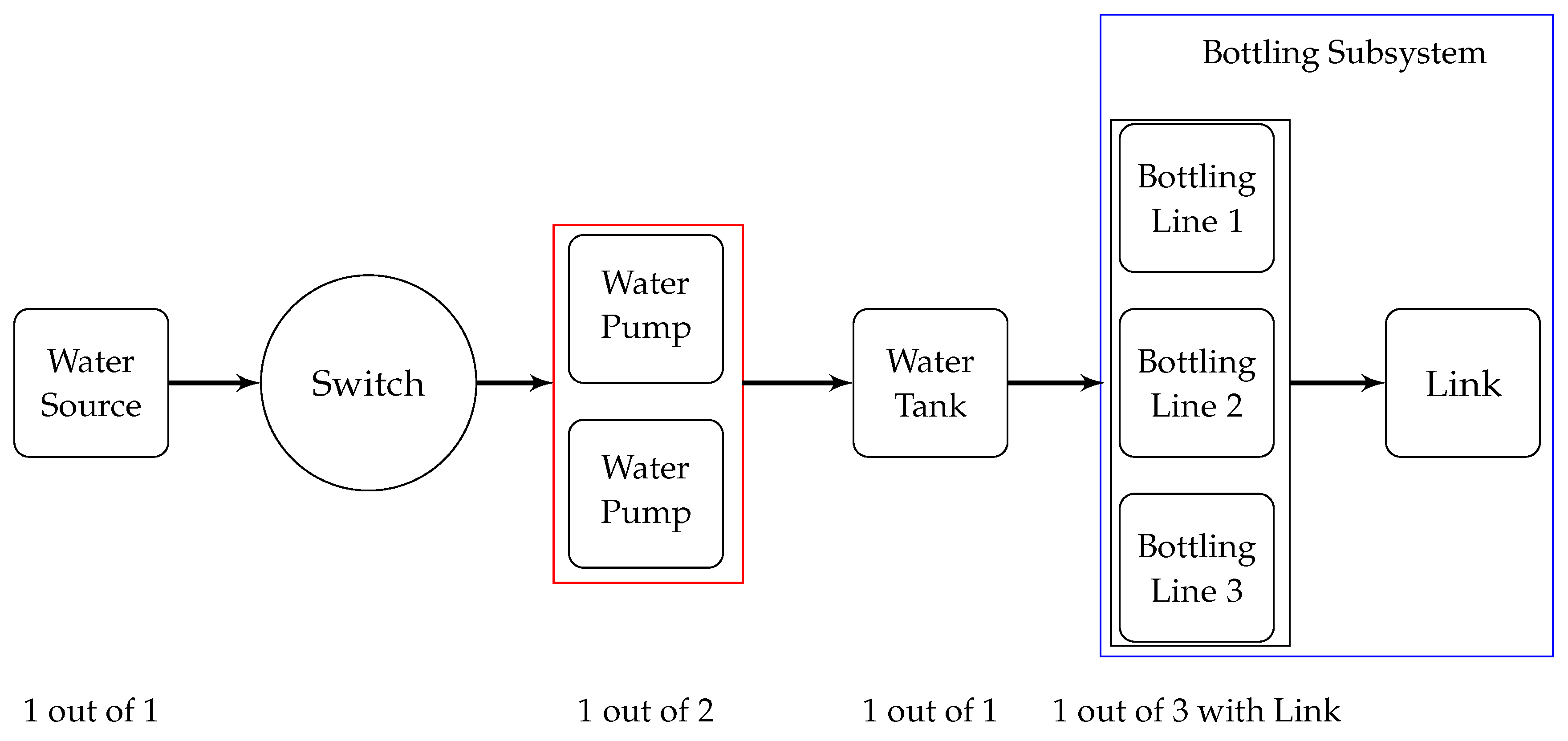
• The system consists of four series-parallel subsystems, as illustrated in Figure 1. In Subsystem 1 (water source), there is a single unit operating in a 1-out-of-1 configuration. Subsystem 2 (water pump) contains two identical units that work in a 1-out-of-2 setup. Subsystem 3 (water tank) has a single unit operating as 1-out-of-1 configuration. Three identical components are stacked in a 1-out-of-3 configuration to form Subsystem 4 (bottling line). Furthermore, failure of the link unit within Subsystem 4 will cause the entire system to become inoperative.
• The system contains a switching device that may be unreliable, and if the switch fails, the system will immediately fail.
• Failures occur at a steady rate throughout time, and this rate is governed by an exponential distribution.
• The Gumbel–Hougard family copula is used to fully restore failed states, whereas the general distribution is used to repair states that have experienced partial failure.
• There have been no reports of damage following the system repair.
• After the repair, the system performs as reliably and efficiently as a new model.

2.3. Notation

t / s: The time parameter that is displayed on a timeline/Representation of each term utilizing the variable associated with the Laplace transform.

${\sigma }_1$/${\sigma }_2$: Failure rates of every unit in Subsystem 1/Subsystem 2

${\sigma }_3$/${\sigma }_4$: Failure rates for Subsystem 3/Subsystem 4

${\sigma }_5$/${\sigma }_{sw}$: Failure rate for the link unit/switch failure rate

$\zeta \left(x\right)$: The repair rates corresponding to the partially failed states of Subsystems 1, 2, 3, and 4

$P_i\left(t\right)$: The possibility of changing from one position or status to another in a particular context.

$\stackrel{*}{P}\left(s\right)$: The Laplace transform is a useful tool for analyzing the probability of transitions between states within a system throughout time.

$P_i(y,t)$: The probability that, at time t, the model will be in a specific state $S_i$ while being influenced by repair procedures determined by the repair parameters y.

$C_1$/$C_2$: Revenue/The cost associated with running the system.

$E_p\left(t\right)$: The expected profit gain from the system’s functioning during the $[0,t]$ interval.

$\nu \left(x\right)$: An expression expressing the joint probability of transitioning from a failed state $S_j$ to a successful state $S_0$, where $j=3,5,6,7,8,9$.

3. The Solution and Model in Mathematics

By examining the observed data or patterns shown in Figure 2, a set of equations was developed. The Markov process concepts were then used to create this system of first-order partial differential equations (see Appendix A for the detailed derivation).

$$\begin{array}{c}\hfill \left[{\displaystyle \frac{d}{dt}}+{\sigma }_1+2{\sigma }_2+{\sigma }_3+3{\sigma }_4+{\sigma }_5+{\sigma }_{sw}\right]P_0\left(t\right)={\int }_0^{\infty }\zeta \left(x\right)P_1(x,t)dx+{\int }_0^{\infty }\zeta \left(y\right)P_4(y,t)dy\\ \hfill +{\int }_0^{\infty }\nu \left(x\right)P_3(x,t)dx+{\int }_0^{\infty }\nu \left(y\right)P_5(y,t)dy+{\int }_0^{\infty }\nu \left(k\right)P_6(k,t)dk+{\int }_0^{\infty }\nu \left(z\right)P_7(z,t)dz\\ \hfill +{\int }_0^{\infty }\nu \left(m\right)P_8(m,t)dm+{\int }_0^{\infty }\nu \left(n\right)P_9(n,t)dn\end{array}$$

(1)

$$\left[{\displaystyle \frac{\mathsf{\partial }}{\mathsf{\partial }t}}+{\displaystyle \frac{\mathsf{\partial }}{\mathsf{\partial }x}}+{\sigma }_1+{\sigma }_3+2{\sigma }_4+{\sigma }_5+{\sigma }_{sw}+\zeta \left(x\right)\right]P_1(x,t)=0$$

(2)

$$\left[{\displaystyle \frac{\mathsf{\partial }}{\mathsf{\partial }t}}+{\displaystyle \frac{\mathsf{\partial }}{\mathsf{\partial }x}}+{\sigma }_1+{\sigma }_3+{\sigma }_4+{\sigma }_5+{\sigma }_{sw}+\zeta \left(x\right)\right]P_2(x,t)=0$$

(3)

$$\left[{\displaystyle \frac{\mathsf{\partial }}{\mathsf{\partial }t}}+{\displaystyle \frac{\mathsf{\partial }}{\mathsf{\partial }x}}+\nu \left(x\right)\right]P_3(x,t)=0$$

(4)

$$\left[{\displaystyle \frac{\mathsf{\partial }}{\mathsf{\partial }t}}+{\displaystyle \frac{\mathsf{\partial }}{\mathsf{\partial }y}}+{\sigma }_1+{\sigma }_2+{\sigma }_3+{\sigma }_5+{\sigma }_{sw}+\zeta \left(y\right)\right]P_4(y,t)=0$$

(5)

$$\left[{\displaystyle \frac{\mathsf{\partial }}{\mathsf{\partial }t}}+{\displaystyle \frac{\mathsf{\partial }}{\mathsf{\partial }y}}+\nu \left(y\right)\right]P_5(y,t)=0$$

(6)

$$\left[{\displaystyle \frac{\mathsf{\partial }}{\mathsf{\partial }t}}+{\displaystyle \frac{\mathsf{\partial }}{\mathsf{\partial }k}}+\nu \left(k\right)\right]P_6(k,t)=0$$

(7)

$$\left[{\displaystyle \frac{\mathsf{\partial }}{\mathsf{\partial }t}}+{\displaystyle \frac{\mathsf{\partial }}{\mathsf{\partial }z}}+\nu \left(z\right)\right]P_7(z,t)=0$$

(8)

$$\left[{\displaystyle \frac{\mathsf{\partial }}{\mathsf{\partial }t}}+{\displaystyle \frac{\mathsf{\partial }}{\mathsf{\partial }m}}+\nu \left(m\right)\right]P_8(m,t)=0$$

(9)

$$\left[{\displaystyle \frac{\mathsf{\partial }}{\mathsf{\partial }t}}+{\displaystyle \frac{\mathsf{\partial }}{\mathsf{\partial }n}}+\nu \left(n\right)\right]P_9(n,t)=0$$

(10)

Boundary conditions:

$$P_1(0,t)=3{\sigma }_4{P}_0\left(t\right)+{\int }_0^{\infty }\zeta \left(x\right)P_2(x,t)dx$$

(11)

$$P_2(0,t)=2{\sigma }_4{P}_1(0,t)$$

(12)

$$P_3(0,t)={\sigma }_4{P}_2(0,t)$$

(13)

$$P_4(0,t)=2{\sigma }_2{P}_0\left(t\right)$$

(14)

$$P_5(0,t)={\sigma }_2{P}_4(0,t)$$

(15)

$$P_6(0,t)={\sigma }_1\left[P_0\left(t\right)+P_i(0,t)\right],i=1,2,4$$

(16)

$$P_7(0,t)={\sigma }_{sw}\left[P_0\left(t\right)+P_i(0,t)\right],i=1,2,4$$

(17)

$$P_8(0,t)={\sigma }_3\left[P_0\left(t\right)+P_i(0,t)\right],i=1,2,4$$

(18)

$$P_9(0,t)={\sigma }_5\left[P_0\left(t\right)+P_i(0,t)\right],i=1,2,4$$

(19)

The initial condition $P_0\left(0\right)=1$, all other transition probabilities are zeros at $t=0$. Equations (1) through (19) are applied to the Laplace transformation, using the boundary conditions, and then solved to yield the Laplace transform of the state transition probabilities.

$$\stackrel{*}{P_0}\left(s\right)={\displaystyle \frac{1}{A\left[s\right]}}$$

(20)

$$\stackrel{*}{P_1}\left(s\right)={\displaystyle \frac{B(1-\stackrel{*}{S_{\zeta }}(s+{\sigma }_1+{\sigma }_3+2{\sigma }_4+{\sigma }_5+{\sigma }_{sw}))}{A\left[s\right](s+{\sigma }_1+{\sigma }_3+2{\sigma }_4+{\sigma }_5+{\sigma }_{sw})}}$$

(21)

$$\stackrel{*}{P_2}\left(s\right)={\displaystyle \frac{2{\sigma }_{4}B(1-\stackrel{*}{S_{\zeta }}(s+{\sigma }_1+{\sigma }_3+{\sigma }_4+{\sigma }_5+{\sigma }_{sw}))}{A\left[s\right](s+{\sigma }_1+{\sigma }_3+{\sigma }_4+{\sigma }_5+{\sigma }_{sw})}}$$

(22)

$$\stackrel{*}{P_3}\left(s\right)={\displaystyle \frac{2{\sigma }_4^{2}B(1-\stackrel{*}{S_{\nu }}\left(s\right))}{\left(s\right)A\left[s\right]}}$$

(23)

$$\stackrel{*}{P_4}\left(s\right)={\displaystyle \frac{2{\sigma }_2(1-\stackrel{*}{S_{\zeta }}(s+{\sigma }_1+{\sigma }_2+{\sigma }_3+{\sigma }_5+{\sigma }_{sw}))}{A\left[s\right](s+{\sigma }_1+{\sigma }_2+{\sigma }_3+{\sigma }_5+{\sigma }_{sw})}}$$

(24)

$$\stackrel{*}{P_5}\left(s\right)={\displaystyle \frac{2{\sigma }_2^2(1-\stackrel{*}{S_{\nu }}\left(s\right))}{\left(s\right)A\left[s\right]}}$$

(25)

$$\stackrel{*}{P_6}\left(s\right)={\displaystyle \frac{{\sigma }_1(1-\stackrel{*}{S_{\nu }}\left(s\right))}{\left(s\right)A\left[s\right]}}\left[1+2{\sigma }_2+B(1+2{\sigma }_4)\right]$$

(26)

$$\stackrel{*}{P_7}\left(s\right)={\displaystyle \frac{{\sigma }_{sw}(1-\stackrel{*}{S_{\nu }}\left(s\right))}{\left(s\right)A\left[s\right]}}\left[1+2{\sigma }_2+B(1+2{\sigma }_4)\right]$$

(27)

$$\stackrel{*}{P_8}\left(s\right)={\displaystyle \frac{{\sigma }_3(1-\stackrel{*}{S_{\nu }}\left(s\right))}{\left(s\right)A\left[s\right]}}\left[1+2{\sigma }_2+B(1+2{\sigma }_4)\right]$$

(28)

$$\stackrel{*}{P_9}\left(s\right)={\displaystyle \frac{{\sigma }_5(1-\stackrel{*}{S_{\nu }}\left(s\right))}{\left(s\right)A\left[s\right]}}\left[1+2{\sigma }_2+B(1+2{\sigma }_4)\right]$$

(29)

where

$$B={\displaystyle \frac{3{\sigma }_4}{1-2{\sigma }_4\left(\stackrel{*}{S_{\zeta }}(s+{\sigma }_1+{\sigma }_3+{\sigma }_4+{\sigma }_5+{\sigma }_{sw})\right)}},$$

(30)

$$\begin{array}{c}A\left[s\right]=s[1+{\displaystyle \frac{(2{\sigma }_4^{2}B+2{\sigma }_2^2)(1-\stackrel{*}{S_{\nu }}\left(s\right))}{s}}+{\displaystyle \frac{2{\sigma }_2(1-\stackrel{*}{S_{\zeta }}(s+{\sigma }_1+{\sigma }_2+{\sigma }_3+{\sigma }_5+{\sigma }_{sw}))}{(s+{\sigma }_1+{\sigma }_2+{\sigma }_3+{\sigma }_5+{\sigma }_{sw})}}\\ +B\left[{\displaystyle \frac{(1-\stackrel{*}{S_{\zeta }}(s+{\sigma }_1+{\sigma }_3+2{\sigma }_4+{\sigma }_5+{\sigma }_{sw}))}{(s+{\sigma }_1+{\sigma }_3+2{\sigma }_4+{\sigma }_5+{\sigma }_{sw})}}+{\displaystyle \frac{2{\sigma }_4(1-\stackrel{*}{S_{\zeta }}(s+{\sigma }_1+{\sigma }_3+{\sigma }_4+{\sigma }_5+{\sigma }_{sw}))}{(s+{\sigma }_1+{\sigma }_3+{\sigma }_4+{\sigma }_5+{\sigma }_{sw})}}\right]\\ +({\sigma }_1+{\sigma }_3+{\sigma }_5+{\sigma }_{sw})\left[1+2{\sigma }_2+B(1+2{\sigma }_4)\right]\left[{\displaystyle \frac{(1-\stackrel{*}{S_{\nu }}\left(s\right))}{s}}\right]]\end{array}$$

(31)

The Laplace transforms below describe the possibilities of system failure and reliable functioning over time:

$${\stackrel{*}{P}}_{up}\left(s\right)=\stackrel{*}{P_0}\left(s\right)+\stackrel{*}{P_1}\left(s\right)+\stackrel{*}{P_2}\left(s\right)+\stackrel{*}{P_4}\left(s\right)$$

(32)

$${\stackrel{*}{P}}_{down}\left(s\right)=1-{\stackrel{*}{P}}_{up}\left(s\right)$$

(33)

4. Analysis of the Model

4.1. Formulating and Analyzing System Availability

Case I: The analysis of availability for the Gumbel–Hougaard family Copula distribution is as follows:

Establish the rates of repair:

$${\stackrel{*}{S}}_{\nu }\left(s\right)={\displaystyle \frac{exp{[x^{\psi }+{\left\{log\zeta \left(x\right)\right\}}^{\psi }]}^{\frac{1}{\psi }}}{s+exp{[x^{\psi }+{\left\{log\zeta \left(x\right)\right\}}^{\psi }]}^{\frac{1}{\psi }}}},{\stackrel{*}{S}}_{\zeta }\left(s\right)={\displaystyle \frac{\zeta }{s+\zeta }},$$

By regarding the various values of the failure as well as repair rate parameter as ${\sigma }_1=0.04,{\sigma }_2=0.05,{\sigma }_3=0.06,{\sigma }_4=0.07,{\sigma }_5=0.08,{\sigma }_{sw}=0.09,\psi =\zeta =x=1$ and $\zeta \left(x\right)=1$ in Equation (32), and subsequently, using the inverse Laplace transform, one can obtain

$$\begin{array}{c}{\stackrel{*}{P}}_{up}\left(t\right)=0.90143+0.133852e^{-3.1624t}-0.0321405e^{-1.56936t}-0.0018855e^{-1.37015t}\\ -0.00125579e^{-1.25446t}-1.35994\left({10}^{-13}\right)e^{-0.41t}+3.55021\left({10}^{-13}\right)e^{-0.34t}\\ -1.80586\left({10}^{-13}\right)e^{-0.32t}\end{array}$$

(34)

Case II: System availability in light of general repair tasks.

General distributions provide a framework for estimating repair rates:

$${\stackrel{*}{S}}_{\nu }\left(s\right)={\displaystyle \frac{\nu }{s+\nu }},{\stackrel{*}{S}}_{\zeta }\left(s\right)={\displaystyle \frac{\zeta }{s+\zeta }}$$

The availability can be calculated as follows by giving the failure and repair rates certain numerical values, shown in Equation (32):

$$\begin{array}{c}{\stackrel{*}{P}}_{up}\left(t\right)=0.770866+0.146155e^{-1.86638t}+0.00517569e^{-1.38095t}+0.00938698e^{-1.26715t}\\ +0.0684161e^{-1.12362t}+1.33004\left({10}^{-13}\right)e^{-0.41t}-1.13835\left({10}^{-13}\right)e^{-0.34t}\\ +1.43186\left({10}^{-13}\right)e^{-0.32t}\end{array}$$

(35)

Case III: Reduction Technique

To adjust the failure rates for the various components, a factor $\rho$ is added, where $0<\rho <1$, and we can increase the model’s availability. This adjustment, compared to the original configuration, results in increased system availability.

$$\begin{array}{c}{\stackrel{*}{P}}_{up}\left(t\right)=0.980367+0.0214923e^{-2.77807t}-0.00171694e^{-1.1228t}-0.0000706093e^{-1.07417t}\\ -0.0000718854e^{-1.05005t}+1.92335\left({10}^{-14}\right)e^{-0.082t}-1.77033\left({10}^{-14}\right)e^{-0.068t}\\ +7.53971\left({10}^{-16}\right)e^{-0.064t}\end{array}$$

(36)

By varying the time variable t from $t=0$ to $t=10$, in Equations (35)–(37), we create the relevant plot in Figure 3 and the data displayed in

Table 2. Comparing the availability of the system in various situations.

Time	Case I	Case II	Case III
0	1	1	1
1	0.899566	0.819661	0.961529
2	0.900053	0.782666	0.960475
3	0.90109	0.77405	0.960756
4	0.901353	0.771794	0.960872
5	0.901413	0.77115	0.960908
6	0.901426	0.770955	0.960918
7	0.901429	0.770895	0.960921
8	0.901429	0.770875	0.960922
9	0.901429	0.770869	0.960923
10	0.90143	0.770867	0.960923

. These findings show how availability changed during the three different scenarios previously discussed.

4.2. Formulating and Analyzing System Reliability

One essential parameter for evaluating the effectiveness of non-repairable systems is reliability. Assuming that the repair rates in Equation (32) are zero. Following this, the result is transformed using the inverse Laplace method.

Case I: The failure fee values listed in Section 4.1 serve as the primary basis for the system’s reliability. This strategy considers equal possibilities and adheres to the same methodology as availability. In essence, we are examining the system’s dependability from a different perspective.

$$R\left(t\right)=-0.74241e^{-0.58t}+1.23529e^{-0.41t}+0.1225e^{-0.34t}+0.384615e^{-0.32t}$$

(37)

Case II: It is anticipated that the failure rates of the system’s additives will drop by a factor of $\rho$, in (0,1), if the reduction approach is implemented. By entering the parameter values from Section 4.1 into Equation (32) and seeing the inverse Laplace transform, this may be demonstrated.

$$R\left(t\right)=-0.64441e^{-0.116t}+1.23529e^{-0.082t}+0.0245e^{-0.068t}+0.384615e^{-0.064t}$$

(38)

As seen in

Table 3. Reliability varies over time in different situations.

Time	Case I	Case II
0	1	1
1	0.770609	0.947872
2	0.576193	0.897254
3	0.422199	0.848292
4	0.305042	0.801091
5	0.218207	0.755726
6	0.154981	0.71224
7	0.109517	0.670657
8	0.0771142	0.630978
9	0.0541674	0.59319
10	0.0379904	0.557266

and the related Figure 4, the reliability values, denoted by R(t), exhibit fluctuation when calculated with Equations (37)–(38).

4.3. Assessment and Formulating Mean Time to Failure

Putting the overall number of repairs to zero and calculating the limit as s approaches zero in Equation (32) will yield the system’s mean time to failure ($MTTF$).

$$MTTF=\underset{s\to 0}{lim}{\stackrel{*}{P}}_{up}\left(s\right)$$

Taking the limit as s approaches zero, and assuming each repair in Equation (32) are insignificant, will yield the formula for $MTTF$.

$$\begin{array}{c}MTTF={\displaystyle \frac{1}{{\sigma }_1+2{\sigma }_2+{\sigma }_3+3{\sigma }_4+{\sigma }_5+{\sigma }_{sw}}}[1+{\displaystyle \frac{2{\sigma }_2}{{\sigma }_1+{\sigma }_2+{\sigma }_3+{\sigma }_5+{\sigma }_{sw}}}\hfill \\ \hfill +3{\sigma }_4\left({\displaystyle \frac{2{\sigma }_4}{{\sigma }_1+{\sigma }_3+{\sigma }_4+{\sigma }_{sw}}}+{\displaystyle \frac{1}{{\sigma }_1+{\sigma }_3+2{\sigma }_4+{\sigma }_5+{\sigma }_{sw}}}\right)]\end{array}$$

(39)

We are analyzing the effect of different parameter values (${\sigma }_1=0.04$, ${\sigma }_2=0.05$, ${\sigma }_3=0.06$, ${\sigma }_4=0.07$, ${\sigma }_5=0.08$, and ${\sigma }_{sw}=0.09$) on the mean time to failure ($MTTF$) by independently varying every parameter. In particular, we are adjusting ${\sigma }_1$, ${\sigma }_2$, ${\sigma }_3$, ${\sigma }_4$, ${\sigma }_5$, and ${\sigma }_{sw}$ across a range from 0.01 to 0.10, as described in Equation (39).

Table 4. Changes in the failure rate significantly impact $MTTF$.

Failure Rates	MTTF (${\mathit{\sigma }}_1$)	MTTF (${\mathit{\sigma }}_2$)	MTTF (${\mathit{\sigma }}_3$)	MTTF (${\mathit{\sigma }}_4$)	MTTF (${\mathit{\sigma }}_5$)	MTTF (${\mathit{\sigma }}_{\mathit{sw}}$)
0.01	3.62236	3.34019	3.87752	4.27994	4.16968	5.93178
0.02	3.50655	3.33961	3.74576	4.23984	4.01849	5.63712
0.03	3.39767	3.33086	3.62236	4.17902	3.87752	5.36959
0.04	3.29511	3.31559	3.50655	4.10749	3.74576	5.1256
0.05	3.19836	3.29511	3.39767	4.03123	3.62236	4.90216
0.06	3.10693	3.2705	3.29511	3.95385	3.50655	4.6968
0.07	3.0204	3.24263	3.19836	3.87752	3.39767	4.50741
0.08	2.93841	3.2122	3.10693	3.80348	3.29511	4.33221
0.09	2.8606	3.1798	3.0204	3.73245	3.19836	4.16968

summarizes the changes in $MTTF$ corresponding to these variances in failure rates, while Figure 5 depicts the same.

4.4. Sensitivity Analysis of the $MTTF$

The partial derivatives of the $MTTF$ with recognize to the failure rates suggest the diploma of sensitivity of the model. Computing the partial derivatives of Equation (39) and replace the values ${\sigma }_1=0.04$, ${\sigma }_2=0.05$, ${\sigma }_3=0.06$, ${\sigma }_4=0.07$, ${\sigma }_5=0.08$, and ${\sigma }_{sw}=0.09$, we obtain the corresponding sensitivity values, which are illustrated in Figure 6 and presented in

Table 5. Variance in sensitivity to shifts in failure rates.

Failure Rates	$\frac{\mathit{\partial }\left(\mathit{MTTF}\right)}{\mathit{\partial }{\mathit{\sigma }}_1}$	$\frac{\mathit{\partial }\left(\mathit{MTTF}\right)}{\mathit{\partial }{\mathit{\sigma }}_2}$	$\frac{\mathit{\partial }\left(\mathit{MTTF}\right)}{\mathit{\partial }{\mathit{\sigma }}_3}$	$\frac{\mathit{\partial }\left(\mathit{MTTF}\right)}{\mathit{\partial }{\mathit{\sigma }}_4}$	$\frac{\mathit{\partial }\left(\mathit{MTTF}\right)}{\mathit{\partial }{\mathit{\sigma }}_5}$	$\frac{\mathit{\partial }\left(\mathit{MTTF}\right)}{\mathit{\partial }{\mathit{\sigma }}_{\mathit{sw}}}$
0.01	−11.9484	0.414756	−13.6212	−1.45843	−15.6658	−16.8632
0.02	−11.224	−0.496713	−12.7443	−3.10996	−14.5905	−15.6658
0.03	−10.5627	−1.22542	−11.9484	−4.0822	−13.6212	−14.5905
0.04	−9.95734	−1.8072	−11.224	−4.6198	−12.7443	−13.6212
0.05	−9.40188	−2.27033	−10.5627	−4.87727	−11.9484	−12.7443
0.06	−8.89097	−2.63722	−9.95734	−4.95397	−11.224	−11.9484
0.07	−8.41999	−2.92577	−9.40188	−4.91468	−10.5627	−11.224
0.08	−7.98492	−3.15037	−8.89097	−4.80215	−9.95734	−10.5627
0.09	−7.58221	−3.32262	−8.41999	−4.64478	−9.40188	−9.95734

.

4.5. Cost Analysis

We can evaluate the expected benefit of the system during the period [0, t) assuming that the service facility remains continuously operational by using the following computation approach:

$$E_p\left(t\right)=C_1{\int }_0^t{P}_{up}\left(t\right)dt-C_{2}t$$

(40)

Case I: If we define $C_1$ as the revenue gained and $C_2$ as the service cost, and we also apply the equivalent parameter values which were used in Equations (34) and (40) from Case I of Section 4.1, then the results will align with those derived in Equation (41). The expected profit values can be shown in

Table 6. Profit expected when the repair adheres to cupola distribution.

Time	${\mathit{C}}_2=0.5$	${\mathit{C}}_2=0.4$	${\mathit{C}}_2=0.3$	${\mathit{C}}_2=0.2$	${\mathit{C}}_2=0.1$
0	0	0	0	0	0
1	0.424006	0.524006	0.624006	0.724006	0.824006
2	0.82331	1.02331	1.22331	1.42331	1.62331
3	1.22398	1.52398	1.82398	2.12398	2.42398
4	1.62524	2.02524	2.42524	2.82524	3.22524
5	2.02663	2.52663	3.02663	3.52663	4.02663
6	2.42805	3.02805	3.62805	4.22805	4.82805
7	2.82948	3.52948	4.22948	4.92948	5.62948
8	3.23091	4.03091	4.83091	5.63091	6.43091
9	3.63233	4.53233	5.43233	6.33233	7.23233
10	4.03376	5.03376	6.03376	7.03376	8.03376

, with a graphical illustration provided in Figure 7.

$$\begin{array}{c}{E}_p\left(t\right)=(0.019469-0.0423261e^{-3.1624t}+0.02048e^{-1.56936t}+0.00137612e^{-1.37015t}\\ +0.00100106e^{-1.25446t}+3.31692\left({10}^{-13}\right)e^{-0.41t}-1.04418\left({10}^{-12}\right)e^{-0.34t}\\ +5.64331\left({10}^{-13}\right)e^{-0.32t}+0.90143t)C_1-C_{2}t\end{array}$$

(41)

Case II: Analyzing costs using a general distribution

Using the equivalent conditions detailed in Section 4.1, Case II, in addition to Equations (35) and (40), the following Equation (42) can be derived. The corresponding expected profit outcomes are summarized in

Table 7. Expected profit assuming a general distribution the repairs.

Time	${\mathit{C}}_2=0.5$	${\mathit{C}}_2=0.4$	${\mathit{C}}_2=0.3$	${\mathit{C}}_2=0.2$	${\mathit{C}}_2=0.1$
0	0	0	0	0	0
1	0.386284	0.486284	0.586284	0.686284	0.786284
2	0.682954	0.882954	1.08295	1.28295	1.48295
3	0.960347	1.26035	1.56035	1.86035	2.16035
4	1.23303	1.63303	2.03303	2.43303	2.83303
5	1.50444	2.00444	2.50444	3.00444	3.50444
6	1.77548	2.37548	2.97548	3.57548	4.17548
7	2.04639	2.74639	3.44639	4.14639	4.84639
8	2.31728	3.11728	3.91728	4.71728	5.51728
9	2.58815	3.48815	4.38815	5.28815	6.18815
10	2.85902	3.85902	4.85902	5.85902	6.85902

, while Figure 8 provides a graphical representation of the data.

$$\begin{array}{c}{E}_p\left(t\right)=(0.150354-0.0783093e^{-1.86638t}-0.00374793e^{-1.38095t}-0.00740793e^{-1.26715t}\\ -0.0608891e^{-1.12362t}-3.24399\left({10}^{-13}\right)e^{-0.41t}+3.34808\left({10}^{-13}\right)e^{-0.34t}\\ -4.47455\left({10}^{-13}\right)e^{-0.32t}+0.770866t)C_1-C_{2}t\end{array}$$

(42)

Case III: Cost analysis with the reduction method

Using the same conditions detailed in Section 4.1, Case III, in addition to Equations (36) and (40), the following Equation (43) can be derived. The corresponding expected profit outcomes are summarized in Table 7, while Figure 8 provides a graphical representation of the data.

$$\begin{array}{c}{E}_p\left(t\right)=(0.960923+0.0461491e^{-2.85061t}-0.00652292e^{-1.24236t}-0.000284645e^{-1.14831t}\\ -0.000264197e^{-1.10053t}-2.05405\left({10}^{-14}\right)e^{-0.164t}+1.21849\left({10}^{-13}\right)e^{-0.136t}\\ -7.11511\left({10}^{-14}\right)e^{-0.128t})C_1-C_{2}t\end{array}$$

(43)

The system’s performance enhanced through the reduction technique, as demonstrated in

Table 8. Expected profit of comparison of three cases.

Time	Origin (${\mathit{C}}_2=0.5$)	General (${\mathit{C}}_2=0.5$)	$\mathit{\rho }=0.4$ (${\mathit{C}}_2=0.5$)
0	0	0	0
1	0.424006	0.386284	0.472112
2	0.82331	0.682954	0.932731
3	1.22398	0.960347	1.39336
4	1.62524	1.23303	1.85418
5	2.02663	1.50444	2.31508
6	2.42805	1.77548	2.77599
7	2.82948	2.04639	3.23691
8	3.23091	2.31728	3.69783
9	3.63233	2.58815	4.15875
10	4.03376	2.85902	4.61968

and Figure 9, for the following values of $C_1=1$; $C_2=0.1$ to $0.5$, throughout a period of time from 0 to 10.

5. Conclusions

This analysis examines the performance metrics of a repairable device consisting of four subsystems connected in collection, where every subsystem contains various numbers of components arranged in parallel. The study, bolstered by way of supplementary variables, shows that adopting copula repair as a restore method proves to be comparatively efficient and powerful. The evaluation supplied in this paper facilitates the identity of a couple of selection-making possibilities. Taking into account varying failure rates, Table 2 and Figure 3 demonstrate how the availability of the system changes with the copula and general repair distribution. They also demonstrate the impact of the reduction method on overall system availability. The data clearly show a decline in the availability of the system over time in all cases. However, it is evident that employing copula repair leads to a relatively higher availability. In Case III, the reduction strategy involves decreasing the system’s unit failure rates via a factor of $\rho$ (with $0<\rho <1$). This targeted reduction aims to increase the system’s overall availability. The assessment of a system’s reliability parallels its availability evaluation in both cases. When time passes, the initial system’s reliability declines due to deliberate adjustments to the failure rates in Case I as well as Case II. Implementing a reduction method with a factor $\rho$ decreases the failure rate per unit, thereby enhancing the system’s overall reliability. Applying this reduction technique greatly increases the original system’s reliability, as seen in Table 3 and Figure 4, especially when comparing Case I and Case II. Figure 5 shows how changes in ${\sigma }_1$, ${\sigma }_2$, ${\sigma }_3$, ${\sigma }_4$, ${\sigma }_5$, and ${\sigma }_{sw}$ impact the system’s ($MTTF$) while all other parameters stay constant. According to the trend found in $MTTF$ across different failure rates, increasing the value of a parameter incrementally reduces the repairable system’s $MTTF$. Table 5 and Figure 6 illustrate that the sensitivity increases with higher failure rate levels. It is vital to recognize that the model becomes more responsive as the failure rate increases. Figure 7 and Figure 8 demonstrate that the expected profit increases over time, with copula repair expected to be more profitable than general repair. This unambiguously indicates that copula repair produces greater profitability through the running of repairable systems while also improving system availability. In Case III, the reduction strategy focuses on lowering the system’s unit failure rates by a factor of $\rho$ (where $0<\rho <1$). This specific reduction aims to enhance the system’s expected profit, as demonstrated in Table 8 and Figure 9. Finally, when service costs rise, profits fall. Researchers may also create a novel model for investigating reliability indicators. Further innovative combinations of series and parallel arrangements may be investigated under improved configuration. This arrangement is used in the majority of industrial and communication systems, and it has promising applications in realistic systems.

References

1. Maihulla, A.S.; Yusuf, I.; Bala, S.I. Performance Evaluation of a Complex Reverse Osmosis Machine System in Water Purification using Reliability, Availability, Maintainability and Dependability Analysis. Reliab. Theory Appl. 2021, 16, 115–131. [Google Scholar]
2. Sadri, S.; Khoshkhoo, R.H.; Ameri, M. Multi objective optimization of reverse osmosis desalination plant with energy approach. J. Mech. Sci. Technol. 2016, 30, 4807–4814. [Google Scholar] [CrossRef]
3. Lee, Y.G.; Lee, Y.S.; Jeon, J.J.; Lee, S.; Yang, D.R. Artificial neural network model for optimizing operation of a seawater reverse osmosis desalination plant. Desalination 2009, 247, 180–189. [Google Scholar] [CrossRef]
4. Ezugbe, E.O.; Rathilal, S. Membrane technologies in wastewater treatment. Membranes 2020, 5, 89. [Google Scholar] [CrossRef]
5. Shalana, L.B.; Kathleen, M.L.; Sherri, L.M. Evaluation of Ozone Pretreatment on Flux Parameters of Reverse Osmosis for Surface Water Treatment. Ozone Sci. Eng. 2008, 30, 152–164. [Google Scholar] [CrossRef]
6. Gulati, J.; Singh, V.V.; Rawal, D.K.; Goel, C.K. Performance analysis of complex system in series configuration under different failure and repair discipline using copula. Int. J. Reliab. Qual. Saf. Eng. 2016, 23, 812–832. [Google Scholar]
7. Yusuf, I.; Hussaini, N. A comparative analysis of three redundant unit systems with three types of failures. Arab. J. Sci. Eng. 2014, 39, 3337–3349. [Google Scholar] [CrossRef]
8. Yusuf, I.; Yusuf, B.; Bala, S.I. Meantime to system failure analysis of a linear consecutive 3-out-of-5 warm standby system in the presence of common cause failure. J. Math. Comput. Sci. 2014, 4, 58–66. [Google Scholar]
9. Gokdere, G.; Keung, H.; Tony, N. Time-dependent reliability analysis for repairable consecutive k-out-of-n: F system. Stat. Theory Rel. Fields 2021, 6, 139–147. [Google Scholar] [CrossRef]
10. Elshoubary, E.E. Effect of reduction method on the performance a software defined network system using Gumbel Hougaard family copula distribution. J. N Soc. Phys. Sci. 2023, 5, 1402. [Google Scholar] [CrossRef]
11. Elshoubary, E.E.; Radwan, T. Studying the Efficiency of the Apache Kafka System Using the Reduction Method, and Its Effectiveness in Terms of Reliability Metrics Subject to a Copula Approach. Appl. Sci. 2024, 14, 6758. [Google Scholar] [CrossRef]
12. Ram, M.; Kumar, A. Performability analysis of a system under 1-out-of-2: G scheme with perfect reworking. J. Braj. Soc. Mech. Sci. Eng. 2015, 37, 1029–1038. [Google Scholar] [CrossRef]
13. Temraz, N. Availability and reliability of a parallel system under imperfect repair and replacement: Analysis and cost optimization. Int. J. Syst. Assur. Eng. Manag. 2019, 10, 1002–1009. [Google Scholar] [CrossRef]
14. Singh, V.V.; Gahlot, M. Reliability analysis of (n) clients system under startopology and copula linguistic approach. Int. J. Comput. Syst. Eng. 2021, 6, 123–133. [Google Scholar] [CrossRef]
15. Anas, S.M.; Yusuf, I. Reliability modeling and performance analysis of reverse osmosis machine in water purification using Gumbel–Hougaard family copula. Life Cycle Reliab. Saf. Eng. 2022, 12, 11–22. [Google Scholar] [CrossRef]
Figure 1. System block design for water bottling.
Axioms 14 00163 g001
Figure 2. Transition flow model.
Axioms 14 00163 g002
Figure 3. Comparison of the availability across three cases.
Axioms 14 00163 g003
Figure 4. Comparison of both cases’ reliability.
Axioms 14 00163 g004
Figure 5. M T T F differences in relation to failure rates.
Axioms 14 00163 g005
Figure 6. System sensitivity study in relation to failure rate.
Axioms 14 00163 g006
Figure 7. Expected profit gains via copula family.
Axioms 14 00163 g007
Figure 8. Expected profit gains via a general repair strategy.
Axioms 14 00163 g008
Figure 9. Expected profit in a variety of cases.
Axioms 14 00163 g009