Influence of a Given Field of Temperature on the Blood Pressure Variation: Variational Analysis, Numerical Algorithms and Simulations

Abstract

This article presents a fluid–elastic structure interaction (FSI) problem when the temperature variation of the two media is also taken into account. We introduced the mathematical description of this interaction in a recent article. Our model includes the coupling between the fluid and the elastic medium equations and, in addition, the coupling with the temperature equations. The novelty of this approach is that we succeed in analyzing a complicated double-coupled problem that allows us to describe more complex physical phenomena both from the theoretical and numerical points of view. Since the main goal of this article is to analyze the influence of an exterior field of temperature on fluid pressure variations, the theoretical results obtained in our previous article are completed with qualitative properties concerning the fluid pressure, such as existence, regularity and uniqueness. Our study continues with approximation schemes: in order to improve the unknowns regularity, we introduce the pressure approximation by a sequence of viscoelastic pressure functions and we prove the weak convergence of this sequence to the pressure; then, we present a numerical approximation scheme with stability and convergence results and Uzawa’s algorithm. The last part of the article is devoted to numerical simulations that rely on the numerical schemes introduced and studied before and highlight some physical phenomena related to the considered problem.

1. Introduction

Fluid–elastic structure interaction is a phenomenon that appears in biology, aerodynamics and other fields of real life and represents a coupled multiphasic problem. Mathematical and numerical analysis of the coupled fluid–elastic structure interaction problem have been topics of interest in the last years. The works presented below have been selected to highlight different approaches from mathematical and numerical points of view regarding FSI problems. In [1,2] existence results are obtained, Refs. [3,4] present an asymptotic analysis, Refs. [5,6] analyze optimal control problems, Refs. [7,8] deal with numerical methods and algorithms, while [9] gives a mathematical introduction to modeling, analysis and simulation techniques for FSI problems.

Our work represents a mathematical and numerical study associated with a simplified model of blood flow through the circulatory system. We consider a thermal FSI problem, which means that in addition to the two coupled models—the incompressible Navier–Stokes system for the fluid and the linear elasticity equations for the elastic structure—we also consider the temperature variation in the two media. Temperature is a physical parameter that plays an important role in many real-life applications. To support this claim, we give two examples of very recent articles dealing with this parameter: [10,11]. So, considering temperature as an additional unknown of the problem on the one hand leads to a mathematical model closer to a physical phenomenon, but, on the other hand, it greatly complicates the mathematical study.

Theoretical studies of FSI problems involving temperature have been published, as far as we know, rarely and only in the last few years (see [12,13,14]). In [12] only the fluid is heat-conducting; the structure does not conduct heat; in [13] a nonlinear interaction problem between a thermoelastic shell and a heat-conducting fluid is considered; the model introduced in [14] deals with a weakly coupled thermal FSI problem; the stationary Navier–Stokes equations for the fluid domain; the convection-diffusion problem for the whole domain and the linear thermoelasticity system in the elastic domain are solved separately. The novelty of our approach is that, unlike the problem studied in [14], we succeed in analyzing, both from mathematical and numerical viewpoints, a fully coupled system with nonlinear equations and nonhomogeneous boundary conditions. In our model the fluid motion is described by the incompressible Navier–Stokes system in the Boussinesq approximation; the behavior of the elastic medium is modeled by the linear thermoelasticity equation and, in addition, the variation in the temperature is given by a convection-diffusion equation corresponding to each medium (nonlinear in the fluid domain). The coupling conditions on the interface between the two media are the continuity of velocities and temperatures, and the continuity of normal stresses, and of heat fluxes.

We introduced this model in [15] where we presented the variational formulation for the thermal FSI model, the approximation results and numerical schemes. The present article represents the second part of our approach to the thermal FSI problem. Since the main purpose of this article is to analyze how the changes in the exterior temperature influence blood pressure variations according to our model, we begin by establishing qualitative properties for the fluid pressure such as existence, regularity and uniqueness.

In order to improve the unknowns regularity, we approximate the variational problem with pressure with a sequence of viscoelastic problems and we prove the weak convergence of the sequence of viscoelastic pressure functions to the pressure.

The next step of the theoretical study is to introduce a suitable numerical approximation scheme and to prove its stability and convergence.

Uzawa’s algorithm allows us to solve the finite-dimensional problem studied before by replacing a functional space with restrictions with a space without restrictions.

The last part of the article is devoted to numerical simulations chosen in order to emphasize physical phenomena related to the considered problem. These simulations rely on the numerical schemes presented before and highlight the following aspects:

• The way in which the changes in the exterior temperature influence the blood pressure variations. For example, Ref. [16] says that high ambient temperatures are associated with lower blood pressure; more specifically systolic blood pressure decreases by 5 mm Hg as the exterior medium temperature increases by 10 °C. Another article, Ref. [17], analyzes in more detail the variation in blood pressure with the variation in exterior temperature. So, when the exterior temperature is between 10 °C and 27 °C, the pressure decreases as the temperature increases, but if the temperature is higher than 27 °C, the pressure increases. Another study, Ref. [18], shows a significant influence of temperature in a closed space on blood pressure variation.
• A comparison between the thermal FSI and FSI models. These simulations highlight the fact that taking into account temperature variations in the two media determines major changes, for example, regarding the longitudinal velocity profile in the fluid.
• The influence of the forces acting in the elastic domain on the fluid longitudinal velocity. This study is of practical interest for the blood flow through vessels, representing one of the most important applications of the FSI. We give two examples that support this assertion. The first example concerns blood flow in venous insufficiency. The blood flow through a leg vein has an anti-gravity sense; when the vein loses its elasticity, this sense is modified, determining the reflux of the blood, which leads to medical complications. These complications are reduced by using elastic stockings. A mathematical analysis of how the compression exerted by the elastic stocking influences blood reflux can be found in [6]. The second example is related to blood flow in stenotic coronary arteries. In [19] the influence of the stenotic coronary arterial wall compliance on the arterial blood flow is analyzed.

2. Presentation of the Mathematical Model

The purpose of this section is to present the mathematical model associated with the thermal FSI problem introduced in [15] and some results and notation from [15], necessary in what follows. The mathematical model describing the FSI consists of the system of equations

$${\displaystyle \left\{\begin{array}{cc}\begin{array}{c}{\rho }_0{\overrightarrow{v}}^{\prime }+{\rho }_0(\overrightarrow{v}·\nabla )\overrightarrow{v}-2\nu \mathrm{div}\left(D\left(\overrightarrow{v}\right)\right)+{\rho }_0{\alpha }_f(T_f-T_{f_0})\overrightarrow{g}+\nabla p={\rho }_0\overrightarrow{g}\hfill \\ \mathrm{div}\overrightarrow{v}=0\hfill \end{array}\hfill & \mathrm{in}{\Omega }_f\times (0,\tau ),\hfill \\ {\rho }_s{\overrightarrow{u}}^{″}-{\displaystyle \sum _{i,j=1}^n}\frac{\partial }{\partial x_i}\left(A_{ij}\frac{\partial \overrightarrow{u}}{\partial x_j}\right)+k{\alpha }_s\nabla (T_s-T_{s_0})={\overrightarrow{f}}_s\hfill & \mathrm{in}{\Omega }_s\times (0,\tau ),\hfill \\ {\rho }_0{c}_f{T}_f^{\prime }+{\rho }_0{c}_f\overrightarrow{v}·\nabla T_f-k_f\Delta T_f=Q_f\hfill & \mathrm{in}{\Omega }_f\times (0,\tau ),\hfill \\ {\rho }_s{c}_s{T}_s^{\prime }+k{\alpha }_s{T}_{s_0}\left(\mathrm{div}{\overrightarrow{u}}^{\prime }\right)-k_s\Delta T_s=Q_s\hfill & \mathrm{in}{\Omega }_s\times (0,\tau ),\hfill \end{array}\right.}$$

(1)

with boundary conditions,

$$\left\{\begin{array}{cc}\overrightarrow{v}=\overrightarrow{0}\hfill & \mathrm{on}{\Gamma }_f\times (0,\tau ),\hfill \\ \overrightarrow{u}=\overrightarrow{0}\hfill & \mathrm{on}{\Gamma }_s\times (0,\tau ),\hfill \\ {\displaystyle \frac{\partial T_f}{\partial n}=0}\hfill & \mathrm{on}{\Gamma }_f\times (0,\tau ),\hfill \\ {\displaystyle \frac{\partial T_s}{\partial n}=0}\hfill & \mathrm{on}{\Gamma }_s^1\times (0,\tau ),\hfill \\ T_s=T_g\hfill & \mathrm{on}{\Gamma }_s^2\times (0,\tau ),\hfill \end{array}\right.$$

(2)

junction conditions,

$$\left\{\begin{array}{c}{\displaystyle \overrightarrow{v}={\overrightarrow{u}}^{\prime }}\hfill \\ {\displaystyle -p\overrightarrow{n}+2\nu D\left(\overrightarrow{v}\right)\overrightarrow{n}={\displaystyle \sum _{i,j=1}^n}{A}_{ij}\frac{\partial \overrightarrow{u}}{\partial x_j}{n}_i-k{\alpha }_s(T_s-T_{s_0})\overrightarrow{n}}\hfill \\ T_f=T_s\hfill \\ {\displaystyle k_f\frac{\partial T_f}{\partial n}=k_s\frac{\partial T_s}{\partial n}}\hfill \end{array}\right.\mathrm{on}\Gamma \times (0,\tau ),$$

(3)

and initial conditions

$$\left\{\begin{array}{cc}\overrightarrow{v}\left(0\right)={\overrightarrow{v}}_0\hfill & \mathrm{in}{\Omega }_f,\hfill \\ \overrightarrow{u}\left(0\right)={\overrightarrow{u}}^{\prime }\left(0\right)=\overrightarrow{0}\hfill & \mathrm{in}{\Omega }_s,\hfill \\ T\left(0\right)=T_0\hfill & \mathrm{in}\Omega .\hfill \end{array}\right.$$

(4)

The unknowns of system (1)–(4) are $\overrightarrow{v}$, p, $T_f$, $\overrightarrow{u}$, $T_s$, representing the fluid velocity, the fluid pressure, the fluid temperature, the displacement and the temperature of the elastic medium, respectively.

The data of the problem are as follows:

• The geometric data: ${\Omega }_f$ (the fluid domain), ${\Omega }_s$ (the solid domain), $\Omega$ (the union of the previous two domains), ${\Gamma }_f$ (the fluid boundary), ${\Gamma }_s$ (the solid boundary), $\Gamma$ (the interface between the two media);
• the positive constants: $\tau$ (which gives the time interval), ${\alpha }_f$, ${\alpha }_s$ (the thermal expansion coefficients corresponding to the two phases), $k_f$, $k_s$ (the thermal conductivities), $c_f$, $c_s$ (the specific heats), ${\rho }_0$, ${\rho }_s$ (the densities), $\nu$ (the fluid viscosity), $k=(3\lambda +2\mu )/3$ (the bulk modulus), where $\lambda$, $\mu$ are the Lamé coefficients;
• the matrix-valued elasticity coefficients $A_{ij}={\left(a_{ij}^{kl}\right)}_{1\le k,l\le n}$, i, $j=1,\dots ,n$ with the following:

  $${\displaystyle a_{ij}^{kl}=\frac{E}{2(1+\sigma )}\left(\frac{2\sigma }{1-2\sigma }{\delta }_{ij}{\delta }_{kl}+{\delta }_{il}{\delta }_{jk}\right),}$$

  where E is a positive constant representing Young’s modulus and ${\displaystyle \sigma \in \left(-1,\frac{1}{2}\right)}$ is a constant representing Poisson’s coefficient. The Lamé constants are linked to the elasticity modulus E and the Poisson ratio $\sigma$ by

  $${\displaystyle \mu =\frac{E}{2(1+\sigma )},\lambda =\frac{E\sigma }{(1+\sigma )(1-2\sigma )};}$$
• $\overrightarrow{g}$ (the gravitational acceleration);
• the functions ${\overrightarrow{v}}_0$ (the initial velocity), $T_0$ (the initial temperature), with $T_{f_0}=T_0{|}_{{\Omega }_f}$, $T_{s_0}=T_0{|}_{{\Omega }_s}$, $Q_f$, $Q_s$ (the internal heat sources), ${\overrightarrow{f}}_s$ (the force in ${\Omega }_s$) and $T_g$ (a given temperature on a part of the elastic domain boundary).

The elements of the elasticity coefficients $A_{ij}$ have the well-known properties

$$\left\{\begin{array}{c}{\displaystyle a_{ij}^{kl}=a_{kj}^{il}=a_{ji}^{lk},\forall i,j,k,l\in \{1,\dots ,n\},}\hfill \\ {\displaystyle \exists \kappa >0\mathrm{s}.\mathrm{t}.{\displaystyle \sum _{i,j,k,l=1}^n}{a}_{ij}^{kl}{\eta }_j^l{\eta }_i^k\ge \kappa {\displaystyle \sum _{j,l=1}^n}{\left({\eta }_j^l\right)}^2,\forall \eta ={\left({\eta }_j^l\right)}_{1\le j,ł\le n},{\eta }_j^l={\eta }_l^j.}\hfill \end{array}\right.$$

Of all the data, the most important role in our problem is played by $T_g$ that appears in ${\left(2\right)}_5$ and represents an exterior field of temperature that acts on a part of the boundary of the coupled domain.

To reduce the number of unknowns of the problem we introduced the functions $\overrightarrow{w}:\overline{\Omega }\times [0,\tau ]\to {\mathbb{R}}^n$ and $T:\overline{\Omega }\times [0,\tau ]\to \mathbb{R}$,

$$\overrightarrow{w}(x,t)=\left\{\begin{array}{cc}\overrightarrow{v}(x,t)\hfill & \mathrm{if}(x,t)\in {\overline{\Omega }}_f\times [0,\tau ],\\ {\overrightarrow{u}}^{\prime }(x,t)\hfill & \mathrm{if}(x,t)\in {\overline{\Omega }}_s\times [0,\tau ],\end{array}\right.$$

(5)

$$T(x,t)=\left\{\begin{array}{cc}{T}_f(x,t)\hfill & \mathrm{if}(x,t)\in {\overline{\Omega }}_f\times [0,\tau ],\\ T_s(x,t)\hfill & \mathrm{if}(x,t)\in {\overline{\Omega }}_s\times [0,\tau ]\end{array}\right.$$

(6)

and then we defined $\overrightarrow{\omega }:\overline{\Omega }\times [0,\tau ]\to {\mathbb{R}}^n$ and $S:\overline{\Omega }\times [0,\tau ]\to \mathbb{R}$:

$$\left\{\begin{array}{c}\overrightarrow{\omega }(x,t)=\overrightarrow{w}(x,t)-{\overrightarrow{w}}_0\left(x\right)\mathrm{in}\overline{\Omega }\times [0,\tau ],\hfill \\ S(x,t)=T(x,t)-{\tilde{T}}_g(x,t)\mathrm{in}\overline{\Omega }\times [0,\tau ],\hfill \end{array}\right.$$

(7)

where ${\tilde{T}}_g:{\Gamma }_s^2\times (0,\tau )\to \mathbb{R}$ represents an extension on $\Omega$ of $T_g$ and has the following properties:

$$\left\{\begin{array}{c}{\tilde{T}}_g\in H^1(0,\tau ;H^1(\Omega ))\cap H^2(0,\tau ;L^2(\Omega )),\hfill \\ {\tilde{T}}_g=T_g\mathrm{on}{\Gamma }_s^2\times (0,\tau ),\hfill \\ {\tilde{T}}_g\left(0\right)=T_0\mathrm{in}\Omega .\hfill \end{array}\right.$$

(8)

The functional spaces necessary for the study of the variational problem considered in [15] are presented below

$$\left\{\begin{array}{c}{\displaystyle \mathcal{W}=\{\overrightarrow{\phi }\in {\left(H_0^1(\Omega )\right)}^n|\mathrm{div}\overrightarrow{\phi }=0\mathrm{in}{\Omega }_f\},}\hfill \\ {\displaystyle \mathcal{H}={\overline{\mathcal{W}}}^{{\parallel ·\parallel }_{{\left(L^2(\Omega )\right)}^n}},}\hfill \\ {\displaystyle {\mathcal{W}}^s=\{\overrightarrow{\phi }\in {\left(H^1\left({\Omega }_s\right)\right)}^n|\overrightarrow{\phi }=\overrightarrow{0}\mathrm{on}{\Gamma }_s\},}\hfill \\ {\displaystyle \mathcal{T}=\{\eta \in H^1(\Omega )|\eta =0\mathrm{on}{\Gamma }_s^2\},}\hfill \\ {\displaystyle H_{\mathcal{W}}=\{\overrightarrow{w}\in L^2(0,\tau ;\mathcal{W})|{\overrightarrow{w}}^{\prime }\in L^2(0,\tau ;{\left(L^2(\Omega )\right)}^n)\},}\hfill \\ {\displaystyle H_{{\mathcal{W}}^s}=\{\overrightarrow{u}\in H^1(0,\tau ;{\mathcal{W}}^s)|{\overrightarrow{u}}^{″}\in L^2(0,\tau ;{\left(L^2\left({\Omega }_s\right)\right)}^n)\},}\hfill \\ {\displaystyle H_{\mathcal{T}}=\{T\in L^2(0,\tau ;\mathcal{T})|T^{\prime }\in L^2(\Omega \times (0,\tau ))\}.}\hfill \end{array}\right.$$

(9)

The units of the variables or constant expressions that appear in (1)–(4) are as follows: m (for ${\overrightarrow{u}}_0$, $\overrightarrow{u}$), m/s (for ${\overrightarrow{v}}_0$, $\overrightarrow{v}$), K (for $T_0$, $T_g$, $T_f$, $T_s$), kg· K⁻¹· m/s³ (for $k_f$, $k_s$), kg/(m· s³) (for $Q_f$, $Q_s$), kg· m/s² (for ${\overrightarrow{f}}_s$), s (for $\tau$), kg/(m·s) (for $\nu$), K⁻¹· m²/s² (for $c_f$, $c_s$), kg/m³ (for ${\rho }_s$, ${\rho }_0$), K⁻¹ (for ${\alpha }_f$, ${\alpha }_s$), kg/(m· s²) (for $A_{ij}$, k, p), m/s² (for $\overrightarrow{g}$).

The variational formulation that follows is written in dimensionless variables, defined as follows: ${\displaystyle {\overrightarrow{x}}^{*}=\frac{\overrightarrow{x}}{L_c}}$, ${\displaystyle t^{*}=\frac{t}{L_c/v_c}}$, ${\displaystyle {\overrightarrow{v}}^{*}=\frac{\overrightarrow{v}}{v_c}}$, ${\displaystyle p^{*}=\frac{p}{{\rho }_0{v}_c^2}}$, ${\displaystyle T^{*}=\frac{T}{T_c}}$, ${\displaystyle {\overrightarrow{g}}^{*}=\frac{\overrightarrow{g}}{v_c^2/L_c}}$, ${\displaystyle {\alpha }_f^{*}=T_c{\alpha }_f}$, ${\displaystyle {\overrightarrow{u}}^{*}=\frac{\overrightarrow{u}}{L_c}}$, ${\displaystyle {\alpha }_s^{*}=T_c{\alpha }_s}$, ${\displaystyle A_{ij}^{*}=\frac{A_{ij}}{{\rho }_s{v}_c^2}}$, ${\displaystyle k^{*}=\frac{k}{{\rho }_s{v}_c^2}}$.

Let us introduce the notation:

$$\left\{\begin{array}{c}{\displaystyle {\chi }_1=\chi \left({\Omega }_f\right)+\frac{{\rho }_s}{{\rho }_0}\chi \left({\Omega }_s\right),}\hfill \\ {\displaystyle {\chi }_2=\chi \left({\Omega }_f\right)+\frac{c_s}{c_f}\frac{{\rho }_s}{{\rho }_0}\chi \left({\Omega }_s\right),}\hfill \\ {\displaystyle {\chi }_3=\frac{1}{\mathrm{Re}{\mathrm{Pr}}_f}\chi \left({\Omega }_f\right)+\frac{c_s}{c_f}\frac{{\rho }_s}{{\rho }_0}\frac{1}{\mathrm{Re}{\mathrm{Pr}}_s}\chi \left({\Omega }_s\right),}\hfill \\ {\displaystyle \overrightarrow{K}\left(t\right)=\chi \left({\Omega }_f\right)\left(\overrightarrow{g}-({\overrightarrow{w}}_0·\nabla ){\overrightarrow{w}}_0+\frac{1}{\mathrm{Re}}\Delta {\overrightarrow{w}}_0-{\alpha }_f({\tilde{T}}_g\left(t\right)-T_0)\overrightarrow{g}\right)}\hfill \\ {\displaystyle +\frac{{\rho }_s}{{\rho }_0}\chi \left({\Omega }_s\right){\overrightarrow{f}}_s\left(t\right)-k{\alpha }_s\frac{{\rho }_s}{{\rho }_0}\nabla ({\tilde{T}}_g\left(t\right)-T_0),}\hfill \\ {\displaystyle {\overrightarrow{K}}_f\left(t\right)=\overrightarrow{g}-({\overrightarrow{w}}_0·\nabla ){\overrightarrow{w}}_0+\frac{1}{\mathrm{Re}}\Delta {\overrightarrow{w}}_0-{\alpha }_f({\tilde{T}}_g\left(t\right)-T_0)\overrightarrow{g}-k{\alpha }_s\frac{{\rho }_s}{{\rho }_0}\nabla ({\tilde{T}}_g-T_0),}\hfill \\ {\displaystyle {\overrightarrow{K}}_s\left(t\right)={\overrightarrow{f}}_s-k{\alpha }_s\nabla ({\tilde{T}}_g-T_0),}\hfill \\ {\displaystyle G\left(t\right)=\chi \left({\Omega }_f\right)Q_f\left(t\right)-{\overrightarrow{w}}_0·\nabla {\tilde{T}}_g\left(t\right)+\frac{c_s}{c_f}\frac{{\rho }_s}{{\rho }_0}\chi \left({\Omega }_s\right)Q_s\left(t\right)-{\chi }_2{\tilde{T}}_g^{\prime }\left(t\right),}\hfill \\ \overrightarrow{F}\left(t\right)={\chi }_3\nabla {\tilde{T}}_g,\hfill \end{array}\right.$$

(10)

where $\chi \left(A\right)$ is the characteristic function of the set A.

The variational problem presented below

$${\displaystyle {\displaystyle \begin{array}{c}\mathrm{Find}(\overrightarrow{\omega },S)\in H_{\mathcal{W}}\times H_{\mathcal{T}}\mathrm{such}\mathrm{that}:\hfill \\ {\int }_{\Omega }{\chi }_1{\overrightarrow{\omega }}^{\prime }\left(t\right)·\overrightarrow{\phi }+{\int }_{{\Omega }_f}(\overrightarrow{\omega }\left(t\right)·\nabla ){\overrightarrow{w}}_0·\overrightarrow{\phi }+{\int }_{{\Omega }_f}({\overrightarrow{w}}_0·\nabla )\overrightarrow{\omega }\left(t\right)·\overrightarrow{\phi }\hfill \\ +\frac{2}{\mathrm{Re}}{\int }_{{\Omega }_f}D\left(\overrightarrow{\omega }\left(t\right)\right):D\left(\overrightarrow{\phi }\right)+{\alpha }_f{\int }_{{\Omega }_f}S\left(t\right)\overrightarrow{g}·\overrightarrow{\phi }+k{\alpha }_s\frac{{\rho }_s}{{\rho }_0}{\int }_{\Omega }\nabla S\left(t\right)·\overrightarrow{\phi }\hfill \\ +\frac{{\rho }_s}{{\rho }_0}{\displaystyle \sum _{i,j=1}^n}{\int }_{{\Omega }_s}{A}_{ij}\frac{\partial }{\partial x_j}\left({\int }_0^t\overrightarrow{\omega }\left(s\right)\mathrm{d}s\right)·\frac{\partial \overrightarrow{\phi }}{\partial x_i}={\int }_{\Omega }\overrightarrow{K}\left(t\right)·\overrightarrow{\phi },\forall \overrightarrow{\phi }\in \mathcal{W}\mathrm{a}.\mathrm{e}.\mathrm{in}(0,\tau ),\hfill \\ {\int }_{\Omega }{\chi }_2{S}^{\prime }\left(t\right)\eta +{\int }_{{\Omega }_f}\eta \overrightarrow{\omega }\left(t\right)·\nabla T_0+{\int }_{{\Omega }_f}\eta {\overrightarrow{w}}_0·\nabla S\left(t\right)+{\int }_{\Omega }{\chi }_3\nabla S\left(t\right)·\nabla \eta \hfill \\ -\frac{c_s}{c_f}\frac{{\rho }_s}{{\rho }_0}\mathrm{E}\mathrm{c}k{\alpha }_s{\int }_{\Omega }\nabla \left(T_0\eta \right)·\overrightarrow{\omega }\left(t\right)={\int }_{\Omega }G\left(t\right)\eta -{\int }_{\Omega }\overrightarrow{F}\left(t\right)·\nabla \eta ,\forall \eta \in \mathcal{T}\mathrm{a}.\mathrm{e}.\mathrm{in}(0,\tau ),\hfill \\ \overrightarrow{\omega }\left(0\right)=\overrightarrow{0}\mathrm{in}\mathcal{H};S\left(0\right)=0\mathrm{in}{L}^2(\Omega ).\hfill \end{array}}}$$

(11)

was studied in [15].

For obtaining more regularity for the function $\overrightarrow{\omega }$, as explained in [15], we considered the family of viscoelastic problems depending on a small parameter $\epsilon >0$

$${\displaystyle \begin{array}{c}\mathrm{Find}({\overrightarrow{\omega }}_{\epsilon },{\overrightarrow{u}}_{\epsilon },S_{\epsilon })\in H_{\mathcal{W}}\times H_{{\mathcal{W}}^s}\times H_{\mathcal{T}}\mathrm{such}\mathrm{that}:\hfill \\ {\int }_{\Omega }{\chi }_1{\overrightarrow{\omega }}_{\epsilon }^{\prime }\left(t\right)·\overrightarrow{\phi }+{\int }_{{\Omega }_f}({\overrightarrow{\omega }}_{\epsilon }\left(t\right)·\nabla ){\overrightarrow{w}}_0·\overrightarrow{\phi }+{\int }_{{\Omega }_f}({\overrightarrow{w}}_0·\nabla ){\overrightarrow{\omega }}_{\epsilon }\left(t\right)·\overrightarrow{\phi }+\frac{2}{\mathrm{Re}}{\int }_{{\Omega }_f}D\left({\overrightarrow{\omega }}_{\epsilon }\left(t\right)\right):D\left(\overrightarrow{\phi }\right)\hfill \\ +{\alpha }_f{\int }_{{\Omega }_f}{S}_{\epsilon }\left(t\right)\overrightarrow{g}·\overrightarrow{\phi }+\frac{{\rho }_s}{{\rho }_0}{\displaystyle \sum _{i,j=1}^n}{\int }_{{\Omega }_s}{A}_{ij}\frac{\partial {\overrightarrow{u}}_{\epsilon }\left(t\right)}{\partial x_j}·\frac{\partial \overrightarrow{\phi }}{\partial x_i}+\epsilon \frac{{\rho }_s}{{\rho }_0}{\displaystyle \sum _{i,j=1}^n}{\int }_{{\Omega }_s}{B}_{ij}\frac{\partial {\overrightarrow{\omega }}_{\epsilon }\left(t\right)}{\partial x_j}·\frac{\partial \overrightarrow{\phi }}{\partial x_i}\hfill \\ +k{\alpha }_s\frac{{\rho }_s}{{\rho }_0}{\int }_{\Omega }\nabla S_{\epsilon }\left(t\right)·\overrightarrow{\phi }={\int }_{\Omega }\overrightarrow{K}\left(t\right)·\overrightarrow{\phi }\forall \overrightarrow{\phi }\in \mathcal{W}\mathrm{a}.\mathrm{e}.\mathrm{in}(0,\tau ),\hfill \\ {\displaystyle \sum _{i,j=1}^n}{\int }_{{\Omega }_s}{A}_{ij}\frac{\partial {\overrightarrow{u}}_{\epsilon }^{\prime }\left(t\right)}{\partial x_j}·\frac{\partial \overrightarrow{\psi }}{\partial x_i}={\displaystyle \sum _{i,j=1}^n}{\int }_{{\Omega }_s}{A}_{ij}\frac{\partial {\overrightarrow{\omega }}_{\epsilon }\left(t\right)}{\partial x_j}·\frac{\partial \overrightarrow{\psi }}{\partial x_i}\forall \overrightarrow{\psi }\in {\mathcal{W}}^s\mathrm{a}.\mathrm{e}.\mathrm{in}(0,\tau ),\hfill \\ {\int }_{\Omega }{\chi }_2{S}_{\epsilon }^{\prime }\left(t\right)\eta +{\int }_{{\Omega }_f}\eta {\overrightarrow{\omega }}_{\epsilon }\left(t\right)·\nabla T_0+{\int }_{{\Omega }_f}\eta {\overrightarrow{w}}_0·\nabla S_{\epsilon }\left(t\right)+{\int }_{\Omega }{\chi }_3\nabla S_{\epsilon }\left(t\right)·\nabla \eta \hfill \\ -\frac{c_s}{c_f}\frac{{\rho }_s}{{\rho }_0}\mathrm{E}\mathrm{c}k{\alpha }_s{\int }_{\Omega }\nabla \left(T_0\eta \right)·{\overrightarrow{\omega }}_{\epsilon }\left(t\right)={\int }_{\Omega }G\left(t\right)\eta -{\int }_{\Omega }\overrightarrow{F}\left(t\right)·\nabla \eta \forall \eta \in \mathcal{T}\mathrm{a}.\mathrm{e}.\mathrm{in}(0,\tau ),\hfill \\ {\overrightarrow{\omega }}_{\epsilon }\left(0\right)=\overrightarrow{0}\mathrm{in}\mathcal{H};{\overrightarrow{u}}_{\epsilon }\left(0\right)=\overrightarrow{0}\mathrm{in}{\mathcal{W}}^s;S_{\epsilon }\left(0\right)=0\mathrm{in}{L}^2(\Omega ).\hfill \end{array}}$$

(12)

In the remainder of this section, we present the elements of the numerical schemes introduced and studied in [15], which are necessary in what follows.

$$\begin{array}{c}{\displaystyle {\mathcal{W}}_h=\left\{{\overrightarrow{\alpha }}_h\in W_h|{\int }_{\mathcal{S}}\mathrm{div}{\overrightarrow{\alpha }}_h\mathrm{d}x=0,\forall \mathcal{S}\in {\mathcal{S}}_h^f\right\},}\hfill \\ {\displaystyle W_h^s=\{{\overrightarrow{\phi }}_h:{\overline{\Omega }}_s\to {\mathbb{R}}^2|{\overrightarrow{\phi }}_h=\overrightarrow{0}\mathrm{on}{\Gamma }_s,{\overrightarrow{\phi }}_h\in {\left(C^0\left({\overline{\Omega }}_s\right)\right)}^2,}\hfill \\ {\displaystyle {\left({\phi }_h\right)}_i{|}_{\mathcal{S}}\mathrm{are}\mathrm{polynomials}\mathrm{of}\mathrm{degree}\le 2,\forall \mathcal{S}\in {\mathcal{S}}_h^s,i=1,2\},}\hfill \\ {\displaystyle {\mathcal{T}}_h=\{{\eta }_h:\overline{\Omega }\to \mathbb{R}|{\eta }_h=0\mathrm{on}{\Gamma }_s^2,{\eta }_h\in C^0\left(\overline{\Omega }\right),}\hfill \\ {\displaystyle {\eta }_h{|}_{\mathcal{S}}\mathrm{is}\mathrm{a}\mathrm{polynomial}\mathrm{of}\mathrm{degree}\le 2,\forall \mathcal{S}\in {\mathcal{S}}_h\},}\hfill \\ {\displaystyle W_h=\{{\overrightarrow{\phi }}_h:\overline{\Omega }\to {\mathbb{R}}^2|{\overrightarrow{\phi }}_h=\overrightarrow{0}\mathrm{on}\partial \Omega ,{\overrightarrow{\phi }}_h\in {\left(C^0\left(\overline{\Omega }\right)\right)}^2,}\hfill \\ {\displaystyle {\left({\phi }_h\right)}_i{|}_{\mathcal{S}}\mathrm{are}\mathrm{polynomials}\mathrm{of}\mathrm{degree}\le 2,\forall \mathcal{S}\in {\mathcal{S}}_h,i=1,2\}}\hfill \end{array}$$

(13)

Consider $N\in {\mathbb{N}}^{*}$, a great parameter and divide the time interval in N intervals of equal length ${\displaystyle \frac{\tau }{N}}$. Let X be a Banach space. We associate to any function $f:[0,\tau ]\to X$, the approximations $f_N^m\in X$, defined by

$$f_N^m=\left\{\begin{array}{cc}{\displaystyle f\left(m\frac{\tau }{N}\right)}\hfill & {\displaystyle \mathrm{if}f\in C^0([0,\tau ];X),}\hfill \\ {\displaystyle \frac{1}{\tau /N}{\int }_{(m-1)\frac{\tau }{N}}^{m\frac{\tau }{N}}f\left(t\right)\mathrm{d}t}\hfill & {\displaystyle \mathrm{if}f\in L^2(0,\tau ;X).}\hfill \end{array}\right.$$

(14)

For a fixed value of $\epsilon$, we associate to the viscoelastic problem (12) the following numerical scheme

$${\displaystyle {\displaystyle \begin{array}{c}\mathrm{For}{\overrightarrow{\omega }}_{h,N}^0,\dots ,{\overrightarrow{\omega }}_{h,N}^{m-1}\in {\mathcal{W}}_h;{\overrightarrow{u}}_{h,N}^0,\dots ,{\overrightarrow{u}}_{h,N}^{m-1}\in W_h^s;S_{h,N}^0,\dots ,S_{h,N}^{m-1}\in {\mathcal{T}}_h\mathrm{given},\hfill \\ {\displaystyle ({\overrightarrow{\omega }}_{h,N}^0,{\overrightarrow{u}}_{h,N}^0,S_{h,N}^0)=(\overrightarrow{0},\overrightarrow{0},0),\mathrm{find}({\overrightarrow{\omega }}_{h,N}^m,{\overrightarrow{u}}_{h,N}^m,S_{h,N}^m)\in {\mathcal{W}}_h\times W_h^s\times {\mathcal{T}}_h\mathrm{s}.\mathrm{t}.}\hfill \\ \frac{1}{\tau /N}{\int }_{\Omega }{\chi }_1{\overrightarrow{\omega }}_{h,N}^m·{\overrightarrow{\phi }}_h+{\int }_{{\Omega }_f}({\overrightarrow{\omega }}_{h,N}^m·\nabla ){\overrightarrow{w}}_0·{\overrightarrow{\phi }}_h+{\int }_{{\Omega }_f}({\overrightarrow{w}}_0·\nabla ){\overrightarrow{\omega }}_{h,N}^m·{\overrightarrow{\phi }}_h\hfill \\ +\frac{2}{\mathrm{Re}}{\int }_{{\Omega }_f}D\left({\overrightarrow{\omega }}_{h,N}^m\right):D\left({\overrightarrow{\phi }}_h\right)+{\alpha }_f{\int }_{{\Omega }_f}{S}_{h,N}^m\overrightarrow{g}·{\overrightarrow{\phi }}_h\hfill \\ +\frac{{\rho }_s}{{\rho }_0}{\displaystyle \sum _{i,j=1}^2}{\int }_{{\Omega }_s}{A}_{ij}\frac{\partial {\overrightarrow{u}}_{h,N}^m}{\partial x_j}·\frac{\partial {\overrightarrow{\phi }}_h}{\partial x_i}+\epsilon \frac{{\rho }_s}{{\rho }_0}{\displaystyle \sum _{i,j=1}^2}{\int }_{{\Omega }_s}{B}_{ij}\frac{\partial {\overrightarrow{\omega }}_{h,N}^m}{\partial x_j}·\frac{\partial {\overrightarrow{\phi }}_h}{\partial x_i}\hfill \\ +k{\alpha }_s\frac{{\rho }_s}{{\rho }_0}{\int }_{\Omega }\nabla S_{h,N}^m·{\overrightarrow{\phi }}_h=\frac{1}{\tau /N}{\int }_{\Omega }{\chi }_1{\overrightarrow{\omega }}_{h,N}^{m-1}·{\overrightarrow{\phi }}_h+{\int }_{\Omega }{\overrightarrow{K}}_N^m·{\overrightarrow{\phi }}_h\forall {\overrightarrow{\phi }}_h\in {\mathcal{W}}_h,\hfill \\ \frac{1}{\tau /N}{\displaystyle \sum _{i,j=1}^2}{\int }_{{\Omega }_s}{A}_{ij}\frac{\partial {\overrightarrow{u}}_{h,N}^m}{\partial x_j}·\frac{\partial {\overrightarrow{\psi }}_h}{\partial x_i}-{\displaystyle \sum _{i,j=1}^2}{\int }_{{\Omega }_s}{A}_{ij}\frac{\partial {\overrightarrow{\omega }}_{h,N}^m}{\partial x_j}·\frac{\partial {\overrightarrow{\psi }}_h}{\partial x_i}\hfill \\ =\frac{1}{\tau /N}{\displaystyle \sum _{i,j=1}^2}{\int }_{{\Omega }_s}{A}_{ij}\frac{\partial {\overrightarrow{u}}_{h,N}^{m-1}}{\partial x_j}·\frac{\partial {\overrightarrow{\psi }}_h}{\partial x_i}\forall {\overrightarrow{\psi }}_h\in W_h^s,\hfill \\ \frac{1}{\tau /N}{\int }_{\Omega }{\chi }_2{S}_{h,N}^m{\eta }_h+{\int }_{{\Omega }_f}({\overrightarrow{\omega }}_{h,N}^m·\nabla T_0){\eta }_h+{\int }_{{\Omega }_f}({\overrightarrow{w}}_0·\nabla S_{h,N}^m){\eta }_h\hfill \\ +{\int }_{\Omega }{\chi }_3\nabla S_{h,N}^m·\nabla {\eta }_h-\frac{c_s}{c_f}\frac{{\rho }_s}{{\rho }_0}\mathrm{E}\mathrm{c}k{\alpha }_s{\int }_{\Omega }\nabla \left(T_0{\eta }_h\right)·{\overrightarrow{\omega }}_{h,N}^m\hfill \\ =\frac{1}{\tau /N}{\int }_{\Omega }{\chi }_2{S}_{h,N}^{m-1}{\eta }_h+{\int }_{\Omega }{G}_N^m{\eta }_h-{\int }_{\Omega }{\overrightarrow{F}}_N^m·\nabla {\eta }_h\forall {\eta }_h\in {\mathcal{T}}_h.\hfill \end{array}}}$$

(15)

where

$$\left\{\begin{array}{c}{\displaystyle {\overrightarrow{\omega }}_{h,N}\in L^2(0,\tau ;{\mathcal{W}}_h),}\hfill \\ {\displaystyle {\overrightarrow{\omega }}_{h,N}\left(t\right)={\overrightarrow{\omega }}_{h,N}^m\mathrm{if}t\in \left[(m-1)\frac{\tau }{N},m\frac{\tau }{N}\right),m=\overline{1,N},}\hfill \end{array}\right.$$

(16)

$$\left\{\begin{array}{c}{\displaystyle {\overrightarrow{u}}_{h,N}\in L^2(0,\tau ;W_h^s),}\hfill \\ {\displaystyle {\overrightarrow{u}}_{h,N}\left(t\right)={\overrightarrow{u}}_{h,N}^m\mathrm{if}t\in \left[(m-1)\frac{\tau }{N},m\frac{\tau }{N}\right),m=\overline{1,N},}\hfill \end{array}\right.$$

(17)

$$\left\{\begin{array}{c}{\displaystyle S_{h,N}\in L^2(0,\tau ;{\mathcal{T}}_h),}\hfill \\ {\displaystyle S_{h,N}\left(t\right)=S_{h,N}^m\mathrm{if}t\in \left[(m-1)\frac{\tau }{N},m\frac{\tau }{N}\right),m=\overline{1,N},}\hfill \end{array}\right.$$

(18)

and

$$\left\{\begin{array}{c}{\displaystyle {\overrightarrow{w}}_{h,N}\in C^0([0,\tau ];{\mathcal{W}}_h),}\hfill \\ {\displaystyle {\overrightarrow{w}}_{h,N}\left(t\right)=({\overrightarrow{\omega }}_{h,N}^m-{\overrightarrow{\omega }}_{h,N}^{m-1})\left(\frac{t}{\tau /N}-m\right)+{\overrightarrow{\omega }}_{h,N}^m,t\in \left[(m-1)\frac{\tau }{N},m\frac{\tau }{N}\right),m=\overline{1,N},}\hfill \end{array}\right.$$

(19)

$$\left\{\begin{array}{c}{\displaystyle {\overrightarrow{\xi }}_{h,N}\in C^0([0,\tau ];W_h^s),}\hfill \\ {\displaystyle {\overrightarrow{\xi }}_{h,N}\left(t\right)=({\overrightarrow{u}}_{h,N}^m-{\overrightarrow{u}}_{h,N}^{m-1})\left(\frac{t}{\tau /N}-m\right)+{\overrightarrow{u}}_{h,N}^m,t\in \left[(m-1)\frac{\tau }{N},m\frac{\tau }{N}\right),m=\overline{1,N},}\hfill \end{array}\right.$$

(20)

$$\left\{\begin{array}{c}{\displaystyle {\sigma }_{h,N}\in C^0([0,\tau ];{\mathcal{T}}_h),}\hfill \\ {\displaystyle {\sigma }_{h,N}\left(t\right)=(S_{h,N}^m-S_{h,N}^{m-1})\left(\frac{t}{\tau /N}-m\right)+S_{h,N}^m,t\in \left[(m-1)\frac{\tau }{N},m\frac{\tau }{N}\right),m=\overline{1,N}.}\hfill \end{array}\right.$$

(21)

Define the following functions:

$$\left\{\begin{array}{c}{\displaystyle {\overrightarrow{\tilde{K}}}_N\in L^2(0,\tau ;{\left(L^2(\Omega )\right)}^2),}\hfill \\ {\displaystyle {\overrightarrow{\tilde{K}}}_N\left(t\right)={\overrightarrow{K}}_N^m\mathrm{for}t\in \left[(m-1)\frac{\tau }{N},m\frac{\tau }{N}\right),m=\overline{1,N},}\hfill \\ {\displaystyle {\tilde{G}}_N\in L^2(0,\tau ;L^2(\Omega )),}\hfill \\ {\displaystyle {\tilde{G}}_N\left(t\right)=G_N^m\mathrm{for}t\in \left[(m-1)\frac{\tau }{N},m\frac{\tau }{N}\right),m=\overline{1,N},}\hfill \\ {\displaystyle {\overrightarrow{\tilde{F}}}_N\in L^2(0,\tau ;{\left(L^2(\Omega )\right)}^2),}\hfill \\ {\displaystyle {\overrightarrow{\tilde{F}}}_N\left(t\right)={\overrightarrow{F}}_N^m\mathrm{for}t\in \left[(m-1)\frac{\tau }{N},m\frac{\tau }{N}\right),m=\overline{1,N}.}\hfill \end{array}\right.$$

(22)

Define the following sets:

$$\left\{\begin{array}{c}{\displaystyle {\mathcal{E}}_{\omega }=\{{\overrightarrow{\omega }}_{h,N},h>0,N\in {\mathbb{N}}^{*},N\ge \widehat{N}\},}\hfill \\ {\displaystyle {\mathcal{E}}_u=\{{\overrightarrow{u}}_{h,N},h>0,N\in {\mathbb{N}}^{*},N\ge \widehat{N}\},}\hfill \\ {\displaystyle {\mathcal{E}}_S=\{S_{h,N},h>0,N\in {\mathbb{N}}^{*},N\ge \widehat{N}\}.}\hfill \end{array}\right.$$

(23)

3. The Variational Problem with Pressure

As can be seen, the variational problem (11), studied in [15], does not contain the fluid pressure. The aim of this section is to introduce fluid pressure and to study its properties. Unlike in the case of Navier–Stokes problems, when the pressure is unique up to an additive constant/function of t, we will prove that in our case the pressure is unique.

In addition to the spaces given by (9) we also define the space

$${\displaystyle \tilde{H}=\{\overrightarrow{\phi }\in L^2(0,\tau ;{\left(H_0^1(\Omega )\right)}^n)|{\overrightarrow{\phi }}^{\prime }\in L^2(0,\tau ;{\left(L^2(\Omega )\right)}^n)\}.}$$

(24)

Theorem 1.

The pair $(\overrightarrow{\omega },S)$ is the unique solution of problem (11) if and only if there exists a unique function $p\in L^2({\Omega }_f\times (0,\tau ))$ such that $(\overrightarrow{\omega },p,S)$ is the solution to the problem:

$${\displaystyle {\displaystyle \begin{array}{c}\mathit{Find}(\overrightarrow{\omega },p,S)\in \tilde{H}\times L^2({\Omega }_f\times (0,\tau ))\times H_{\mathcal{T}}\mathit{such}\mathit{that}:\hfill \\ {\displaystyle {\int }_{\Omega }{\chi }_1{\overrightarrow{\omega }}^{\prime }·\overrightarrow{\phi }+{\int }_{{\Omega }_f}(\overrightarrow{\omega }·\nabla ){\overrightarrow{w}}_0·\overrightarrow{\phi }+{\int }_{{\Omega }_f}({\overrightarrow{w}}_0·\nabla )\overrightarrow{\omega }·\overrightarrow{\phi }+\frac{2}{\mathit{Re}}{\int }_{{\Omega }_f}D\left(\overrightarrow{\omega }\right):D\left(\overrightarrow{\phi }\right)}\hfill \\ {\displaystyle +{\alpha }_f{\int }_{{\Omega }_f}S\overrightarrow{g}·\overrightarrow{\phi }+\frac{{\rho }_s}{{\rho }_0}{\displaystyle \sum _{i,j=1}^n}{\int }_{{\Omega }_s}{A}_{ij}\frac{\partial }{\partial x_j}\left({\int }_0^t\overrightarrow{\omega }\left(s\right)\mathit{ds}\right)·\frac{\partial \overrightarrow{\phi }}{\partial x_i}}\hfill \\ {\displaystyle +k{\alpha }_s\frac{{\rho }_s}{{\rho }_0}{\int }_{\Omega }\nabla S·\overrightarrow{\phi }+k{\alpha }_s\frac{{\rho }_s}{{\rho }_0}{\int }_{{\Omega }_f}\mathit{Sdiv}\overrightarrow{\phi }-{\int }_{{\Omega }_f}\mathit{pdiv}\overrightarrow{\phi }={\int }_{\Omega }\overrightarrow{K}·\overrightarrow{\phi }}\hfill \\ {\displaystyle -k{\alpha }_s\frac{{\rho }_s}{{\rho }_0}{\int }_{{\Omega }_f}({\tilde{T}}_g-T_0)\mathit{div}\overrightarrow{\phi },\forall \overrightarrow{\phi }\in {\left(H_0^1(\Omega )\right)}^{n}a.e.\mathit{in}(0,\tau ),}\hfill \\ {\int }_{\Omega }{\chi }_2{S}^{\prime }\eta +{\int }_{{\Omega }_f}\eta \overrightarrow{\omega }·\nabla T_0+{\int }_{{\Omega }_f}\eta {\overrightarrow{w}}_0·\nabla S+{\int }_{\Omega }{\chi }_3\nabla S·\nabla \eta \hfill \\ -\frac{c_s}{c_f}\frac{{\rho }_s}{{\rho }_0}\mathit{Ec}k{\alpha }_s{\int }_{\Omega }\nabla \left(T_0\eta \right)·\overrightarrow{\omega }={\int }_{\Omega }G\eta -{\int }_{\Omega }\overrightarrow{F}·\nabla \eta ,\forall \eta \in \mathcal{T}a.e.\mathit{in}(0,\tau ),\hfill \\ {\int }_{{\Omega }_f}\mathit{qdiv}\overrightarrow{\omega }=0,\forall q\in L^2\left({\Omega }_f\right)a.e.\mathit{in}(0,\tau ),\hfill \\ \overrightarrow{\omega }\left(0\right)=\overrightarrow{0}\mathit{in}\mathcal{H};S\left(0\right)=0\mathit{in}{L}^2(\Omega ).\hfill \end{array}}}$$

(25)

Proof. 

1. If we take in (25) a test function $\overrightarrow{\phi }\in \mathcal{W}$, we obtain that $(\overrightarrow{\omega },S)$ is the solution for (11).

2. Suppose next that $(\overrightarrow{\omega },S)$ is the unique solution for (25).

Considering the space

$$\mathcal{V}=\left\{\overrightarrow{\psi }\in {\left(\mathcal{D}\left({\Omega }_f\right)\right)}^n|\mathrm{div}\overrightarrow{\psi }=0\right\}$$

(26)

we notice that for all $\overrightarrow{\psi }\in \mathcal{V}$, the function $\overrightarrow{\phi }=\overrightarrow{\psi }$ in ${\overline{\Omega }}_f$, $\overrightarrow{\phi }=\overrightarrow{0}$ in ${\overline{\Omega }}_s$ is a test function for ${\left(11\right)}_2$, which means that

$$\begin{array}{c}{\displaystyle {\int }_{\Omega }{\overrightarrow{\omega }}^{\prime }·\overrightarrow{\psi }+{\int }_{{\Omega }_f}(\overrightarrow{\omega }·\nabla ){\overrightarrow{w}}_0·\overrightarrow{\psi }+{\int }_{{\Omega }_f}({\overrightarrow{w}}_0·\nabla )\overrightarrow{\omega }·\overrightarrow{\psi }+\frac{2}{\mathrm{Re}}{\int }_{{\Omega }_f}D\left(\overrightarrow{\omega }\right):D\left(\overrightarrow{\psi }\right)}\\ {\displaystyle +{\alpha }_f{\int }_{{\Omega }_f}S\overrightarrow{g}·\overrightarrow{\psi }+k{\alpha }_s\frac{{\rho }_s}{{\rho }_0}{\int }_{{\Omega }_f}\nabla S·\overrightarrow{\psi }={\int }_{{\Omega }_f}{\overrightarrow{K}}_f·\overrightarrow{\psi },\forall \overrightarrow{\psi }\in \mathcal{V}\mathrm{in}{L}^2(0,\tau ).}\end{array}$$

(27)

Denoting

$${\displaystyle \overrightarrow{F}={\overrightarrow{\omega }}^{\prime }+(\overrightarrow{\omega }·\nabla ){\overrightarrow{w}}_0+({\overrightarrow{w}}_0·\nabla )\overrightarrow{\omega }-\frac{2}{\mathrm{Re}}\mathrm{div}\left(D\left(\overrightarrow{\omega }\right)\right)+{\alpha }_{f}S\overrightarrow{g}-{\overrightarrow{K}}_f}$$

(28)

and taking into account the regularity of the terms from the right-hand side of (28), it follows that

$${\displaystyle \overrightarrow{F}\in L^2(0,\tau ;{\left(H^{-1}\left({\Omega }_f\right)\right)}^n).}$$

(29)

Integrating by parts the fourth and the sixth terms in (27) and using (29), (27) becomes

$${\displaystyle {\langle \overrightarrow{F}\left(t\right),\overrightarrow{\psi }\rangle }_{{\mathcal{V}}^{\prime },\mathcal{V}}=0,\forall \overrightarrow{\psi }\in \mathcal{V}\mathrm{a}.\mathrm{e}.\mathrm{i}\mathrm{n}(0,\tau ).}$$

(30)

Using Prop. 1.1 and Prop. 1.2 of [20], Chap. 1, we introduce a distribution q such that

$${\displaystyle \overrightarrow{F}=-\nabla q\mathrm{in}{L}^2(0,\tau ;{\left(H^{-1}\left({\Omega }_f\right)\right)}^n)}$$

(31)

and

$${\displaystyle q\in L^2({\Omega }_f\times (0,\tau )).}$$

(32)

Supposing that there are two functions $q_1$, $q_2$, $q_1\ne q_2$ that verify (31) and (32) it follows that

$${\displaystyle q_1-q_2=\alpha \mathrm{in}{L}^2(0,\tau ).}$$

(33)

Relation (31) may be written as

$${\langle \overrightarrow{F}\left(t\right)+\nabla q\left(t\right),\zeta \rangle }_{{\left(H^{-1}\left({\Omega }_f\right)\right)}^n,{\left(H_0^1\left({\Omega }_f\right)\right)}^n}=0,\forall \zeta \in {\left(H_0^1\left({\Omega }_f\right)\right)}^n\mathrm{a}.\mathrm{e}.\mathrm{i}\mathrm{n}(0,\tau ).$$

(34)

Using the density of ${\left(H_0^1\left({\Omega }_f\right)\right)}^n$ in ${\left(L^2\left({\Omega }_f\right)\right)}^n$ we can extend the functional $\overrightarrow{F}\left(t\right)+\nabla q\left(t\right)$ from ${\left(H_0^1\left({\Omega }_f\right)\right)}^n$ to ${\left(L^2\left({\Omega }_f\right)\right)}^n$ and hence for a.e. $t\in (0,\tau )$

$${\displaystyle {\langle \overrightarrow{F}\left(t\right)+\nabla q\left(t\right),\zeta \rangle }_{{\left(H^{-1}\left({\Omega }_f\right)\right)}^n,{\left(H_0^1\left({\Omega }_f\right)\right)}^n}={\int }_{{\Omega }_f}(\overrightarrow{F}\left(t\right)+\nabla q\left(t\right))·\overrightarrow{\zeta },\forall \overrightarrow{\zeta }\in {\left(H_0^1(\Omega )\right)}^n.}$$

(35)

From (34) and (35) and using again the density of ${\left(H_0^1\left({\Omega }_f\right)\right)}^n$ in ${\left(L^2\left({\Omega }_f\right)\right)}^n$ we obtain

$${\displaystyle {\int }_{{\Omega }_f}(\overrightarrow{F}\left(t\right)+\nabla q\left(t\right))·\overrightarrow{\zeta }=0,\forall \overrightarrow{\zeta }\in {\left(L^2\left({\Omega }_f\right)\right)}^n.}$$

(36)

Let us define

$${\displaystyle {\mathcal{V}}^f=\left\{\overrightarrow{\rho }\in {\left(H^1\left({\Omega }_f\right)\right)}^n|\overrightarrow{\rho }=\overrightarrow{0}\mathrm{on}{\Gamma }_f\right\}.}$$

(37)

Since ${\mathcal{V}}^f\subset {\left(L^2\left({\Omega }_f\right)\right)}^n$, we can take in (36) $\overrightarrow{\zeta }\in {\mathcal{V}}^f$, that yields

$${\displaystyle {\int }_{{\Omega }_f}(\overrightarrow{F}\left(t\right)+\nabla q\left(t\right))·\overrightarrow{\zeta }=0,\forall \overrightarrow{\zeta }\in {\mathcal{V}}^f.}$$

(38)

Let $\Omega \subset {\mathbb{R}}^n$ open, bounded with $\partial \Omega$ Lipschitz. Denote

$${\displaystyle T(\Omega )=\left\{\mathcal{S}\in {\left(L^2(\Omega )\right)}^{n\times n}|\mathrm{div}\mathcal{S}\in {\left(L^2(\Omega )\right)}^n\right\},}$$

(39)

the trace operator

$${\displaystyle {\gamma }_0:{\left(H^1(\Omega )\right)}^n\to {\left(H^{1/2}(\partial \Omega )\right)}^n}$$

(40)

and

$${\displaystyle {\gamma }_{\nu }:T(\Omega )\to {\left(H^{-1/2}(\partial \Omega )\right)}^n,{\gamma }_{\nu }\mathcal{S}=\mathcal{S}\overrightarrow{n}.}$$

(41)

For calculating ${\displaystyle {\int }_{{\Omega }_f}\mathrm{div}\left(\frac{2}{\mathrm{Re}}D\left(\overrightarrow{\omega }\left(t\right)\right)-q\left(t\right)I\right)·\overrightarrow{\rho }}$ for $\overrightarrow{\rho }\in {\mathcal{V}}^f$ we will use the following generalized Stokes formula:

$$\begin{array}{c}{\displaystyle {\int }_{\Omega }\left(\mathcal{S}:\nabla \overrightarrow{\phi }+\overrightarrow{\phi }·\mathrm{div}\mathcal{S}\right)={\langle {\gamma }_{\nu }\mathcal{S},{\gamma }_0\overrightarrow{\phi }\rangle }_{{\left(H^{-1/2}(\partial \Omega )\right)}^n,{\left(H^{1/2}(\partial \Omega )\right)}^n}}\\ {\displaystyle \forall \overrightarrow{\phi }\in {\left(H^1(\Omega )\right)}^n,\forall \mathcal{S}\in T(\Omega ).}\end{array}$$

(42)

Relation (31) can also be written as

$${\displaystyle {\overrightarrow{\omega }}^{\prime }+(\overrightarrow{\omega }·\nabla ){\overrightarrow{w}}_0+({\overrightarrow{w}}_0·\nabla )\overrightarrow{\omega }+{\alpha }_{f}S\overrightarrow{g}-{\overrightarrow{K}}_f=\mathrm{div}\left(\frac{2}{\mathrm{Re}}-qI\right)\mathrm{in}{L}^2(0,\tau ;{\left(H^{-1}(\Omega )\right)}^n)}$$

and, taking into account the regularity of the left-hand, it follows that

$${\displaystyle \mathrm{div}\left(\frac{2}{\mathrm{Re}}D\left(\overrightarrow{\omega }\right)-qI\right)\in L^2(0,\tau ;{\left(L^2\left({\Omega }_f\right)\right)}^n).}$$

(43)

Applying next (42) for ${\displaystyle \mathcal{S}=\frac{2}{\mathrm{Re}}D\left(\overrightarrow{\omega }\left(t\right)\right)-q\left(t\right)I}$, $\overrightarrow{\phi }=\overrightarrow{\rho }\in {\mathcal{V}}^f$ we obtain a.e. in $(0,\tau )$

$$\begin{array}{c}{\displaystyle {〈\mathrm{div}\left(q\left(t\right)I-\frac{2}{\mathrm{Re}}D\left(\overrightarrow{\omega }\left(t\right)\right)\right),\overrightarrow{\rho }〉}_{{\left({\mathcal{V}}^f\right)}^{\prime },{\mathcal{V}}^f}}\\ {\displaystyle ={\int }_{{\Omega }_f}\overrightarrow{\rho }·\mathrm{div}\left(q\left(t\right)I-\frac{2}{\mathrm{Re}}D\left(\overrightarrow{\omega }\left(t\right)\right)\right)=\frac{2}{\mathrm{Re}}{\int }_{{\Omega }_f}D\left(\overrightarrow{\omega }\left(t\right)\right):D\left(\overrightarrow{\rho }\right)}\\ {\displaystyle -{\int }_{{\Omega }_f}q\left(t\right)\mathrm{div}\overrightarrow{\rho }+{〈q\left(t\right)\overrightarrow{n}-\frac{2}{\mathrm{Re}}D\left(\overrightarrow{\omega }\left(t\right)\right)\overrightarrow{n},\overrightarrow{\rho }〉}_{{\left(H^{-1/2}(\Gamma )\right)}^n,{\left(H^{-1/2}(\Gamma )\right)}^n}\forall \overrightarrow{\rho }\in {\mathcal{V}}^f.}\end{array}$$

(44)

Using the previous relation, (27) becomes

$$\begin{array}{c}{\displaystyle {\int }_{{\Omega }_f}{\overrightarrow{\omega }}^{\prime }·\overrightarrow{\rho }+{\int }_{{\Omega }_f}(\overrightarrow{\omega }·\nabla ){\overrightarrow{w}}_0·\overrightarrow{\rho }+{\int }_{{\Omega }_f}({\overrightarrow{w}}_0·\nabla )\overrightarrow{\omega }·\overrightarrow{\rho }+{\alpha }_f{\int }_{{\Omega }_f}S\overrightarrow{g}·\overrightarrow{\rho }}\\ {\displaystyle -{\int }_{{\Omega }_f}{\overrightarrow{K}}_f·\overrightarrow{\rho }+\frac{2}{\mathrm{Re}}{\int }_{{\Omega }_f}D\left(\overrightarrow{\omega }\right):D\left(\overrightarrow{\rho }\right)-{\int }_{{\Omega }_f}q\left(t\right)\mathrm{div}\overrightarrow{\rho }}\\ {\displaystyle +{〈q\left(t\right)\overrightarrow{n}-\frac{2}{\mathrm{Re}}D\left(\overrightarrow{\omega }\left(t\right)\right)\overrightarrow{n},\overrightarrow{\rho }〉}_{{\left(H^{-1/2}(\Gamma )\right)}^n,{\left(H^{-1/2}(\Gamma )\right)}^n}=0,\forall \overrightarrow{\rho }\in {\mathcal{V}}^f\mathrm{in}{L}^2(0,\tau ).}\end{array}$$

(45)

Proceeding in the same way for ${\Omega }_s$ we obtain a.e. in $(0,\tau )$

$$\begin{array}{c}{\displaystyle \frac{{\rho }_s}{{\rho }_0}{\int }_{{\Omega }_s}{\overrightarrow{\omega }}^{\prime }·\overrightarrow{\rho }+\frac{{\rho }_s}{{\rho }_0}{\displaystyle \sum _{i,j=1}^n}{\int }_{{\Omega }_s}{A}_{ij}\frac{\partial }{\partial x_j}\left({\int }_0^t\overrightarrow{\omega }\left(s\right)\mathrm{d}s\right)·\frac{\partial \overrightarrow{\rho }}{\partial x_i}}\\ {\displaystyle +\frac{{\rho }_s}{{\rho }_0}{〈{\displaystyle \sum _{i,j=1}^n}{A}_{ij}\frac{\partial }{\partial x_j}\left({\int }_0^t\overrightarrow{\omega }\left(s\right)\mathrm{d}s\right)n_i,\overrightarrow{\rho }〉}_{{\left(H^{-1/2}(\Gamma )\right)}^n,{\left(H^{1/2}(\Gamma )\right)}^n}}\\ {\displaystyle +k{\alpha }_s\frac{{\rho }_s}{{\rho }_0}{\int }_{{\Omega }_s}\nabla S\left(t\right)·\overrightarrow{\rho }=\frac{{\rho }_s}{{\rho }_0}{\int }_{{\Omega }_s}{\overrightarrow{K}}_s\left(t\right)·\overrightarrow{\rho },\forall \overrightarrow{\rho }\in {\mathcal{V}}^s\mathrm{in}{L}^2(0,\tau )}\end{array}$$

(46)

with

$${\displaystyle {\mathcal{V}}^s=\{\overrightarrow{\rho }\in {\left(H^1\left({\Omega }_s\right)\right)}^n|\overrightarrow{\rho }=\overrightarrow{0}\mathrm{on}{\Gamma }_s\}.}$$

(47)

Consider $\overrightarrow{\phi }\in {\left(H_0^1(\Omega )\right)}^n$. Taking as a test function $\overrightarrow{\phi }{|}_{{\Omega }_f}$ in (45) and $\overrightarrow{\phi }{|}_{{\Omega }_s}$ in (46) and adding the two relations we obtain a.e. in $(0,\tau )$

$$\begin{array}{c}{\displaystyle {\int }_{\Omega }{\chi }_1{\overrightarrow{\omega }}^{\prime }\left(t\right)·\overrightarrow{\phi }+{\int }_{{\Omega }_f}(\overrightarrow{\omega }\left(t\right)·\nabla ){\overrightarrow{w}}_0·\overrightarrow{\phi }+{\int }_{{\Omega }_f}({\overrightarrow{w}}_0·\nabla )\overrightarrow{\omega }\left(t\right)·\overrightarrow{\phi }}\\ {\displaystyle +\frac{2}{\mathrm{Re}}{\int }_{{\Omega }_f}D\left(\overrightarrow{\omega }\left(t\right)\right):D\left(\overrightarrow{\phi }\right)+{\alpha }_f{\int }_{{\Omega }_f}S\left(t\right)\overrightarrow{g}·\overrightarrow{\phi }-{\int }_{{\Omega }_f}q\left(t\right)\mathrm{div}\overrightarrow{\phi }}\\ {\displaystyle +k{\alpha }_s\frac{{\rho }_s}{{\rho }_0}{\int }_{{\Omega }_s}\nabla S\left(t\right)·\overrightarrow{\phi }+\frac{{\rho }_s}{{\rho }_0}{\displaystyle \sum _{i,j=1}^n}{\int }_{{\Omega }_s}{A}_{ij}\frac{\partial }{\partial x_j}\left({\int }_0^t\overrightarrow{\omega }\left(s\right)\mathrm{d}s\right)·\frac{\partial \overrightarrow{\phi }}{\partial x_i}}\\ {\displaystyle +{〈q\left(t\right)\overrightarrow{n}-\frac{2}{\mathrm{Re}}D\left(\overrightarrow{\omega }\left(t\right)\right)\overrightarrow{n},\overrightarrow{\phi }〉}_{{\left(H^{-1/2}(\Gamma )\right)}^n,{\left(H^{-1/2}(\Gamma )\right)}^n}}\\ {\displaystyle +\frac{{\rho }_s}{{\rho }_0}{〈{\displaystyle \sum _{i,j=1}^n}{A}_{ij}\frac{\partial }{\partial x_j}\left({\int }_0^t\overrightarrow{\omega }\left(s\right)\mathrm{d}s\right)n_i,\overrightarrow{\phi }〉}_{{\left(H^{-1/2}(\Gamma )\right)}^n,{\left(H^{1/2}(\Gamma )\right)}^n}}\\ {\displaystyle ={\int }_{\Omega }\left(\chi \left({\Omega }_f\right){\overrightarrow{K}}_f\left(t\right)+\frac{{\rho }_s}{{\rho }_0}\chi \left({\Omega }_s\right){\overrightarrow{K}}_s\left(t\right)\right)·\overrightarrow{\phi },\forall \overrightarrow{\phi }\in {\left(H_0^1(\Omega )\right)}^n\mathrm{in}{L}^2(0,\tau ).}\end{array}$$

(48)

An easy calculation gives

$$\begin{array}{c}{\displaystyle k{\alpha }_s\frac{{\rho }_s}{{\rho }_0}{\int }_{{\Omega }_s}\nabla S\left(t\right)·\overrightarrow{\phi }=k{\alpha }_s\frac{{\rho }_s}{{\rho }_0}{\int }_{\Omega }\nabla S\left(t\right)·\overrightarrow{\phi }+k{\alpha }_s\frac{{\rho }_s}{{\rho }_0}{\int }_{{\Omega }_f}S\left(t\right)\mathrm{div}\overrightarrow{\phi }}\\ {\displaystyle -k{\alpha }_s\frac{{\rho }_s}{{\rho }_0}{\langle S\left(t\right)\overrightarrow{n},\overrightarrow{\phi }\rangle }_{{\left(H^{-1/2}(\Gamma )\right)}^n,{\left(H^{1/2}(\Gamma )\right)}^n}.}\end{array}$$

(49)

Taking into account the Expression ${\left(10\right)}_{4–6}$, the right-hand side of (48) may be written as

$$\begin{array}{c}{\displaystyle {\int }_{\Omega }\left(\chi \left({\Omega }_f\right){\overrightarrow{K}}_f\left(t\right)+\frac{{\rho }_s}{{\rho }_0}\chi \left({\Omega }_s\right){\overrightarrow{K}}_s\left(t\right)\right)·\overrightarrow{\phi }={\int }_{\Omega }\overrightarrow{K}\left(t\right)·\overrightarrow{\phi }}\\ {\displaystyle -k{\alpha }_s\frac{{\rho }_s}{{\rho }_0}{\int }_{{\Omega }_f}({\tilde{T}}_g\left(t\right)-T_0)\mathrm{div}\overrightarrow{\phi }+k{\alpha }_s\frac{{\rho }_s}{{\rho }_0}{\langle ({\tilde{T}}_g\left(t\right)-T_0)\overrightarrow{n},\overrightarrow{\phi }\rangle }_{{\left(H^{-1/2}(\Gamma )\right)}^n,{\left(H^{1/2}(\Gamma )\right)}^n}.}\end{array}$$

(50)

Notice that the normal that appears in (48)–(50) is exterior to ${\Omega }_f$.

Introducing (49) and (50) in (48) and using ${\left(11\right)}_2$ we obtain

$$\begin{array}{c}{\displaystyle {〈q\left(t\right)\overrightarrow{n}-\frac{2}{\mathrm{Re}}D\left(\overrightarrow{\omega }\left(t\right)\right)\overrightarrow{n},\overrightarrow{\phi }〉}_{{\left(H^{-1/2}(\partial {\Omega }_f)\right)}^n,{\left(H^{1/2}(\partial {\Omega }_f)\right)}^n}}\\ {\displaystyle +\frac{{\rho }_s}{{\rho }_0}\langle {\displaystyle \sum _{i,j=1}^n}{A}_{ij}\frac{\partial }{\partial x_j}\left({\int }_0^t\overrightarrow{\omega }\left(s\right)\mathrm{d}s\right)n_i}\\ {\displaystyle -k{\alpha }_s(S\left(t\right)+{\tilde{T}}_g\left(t\right)-T_0)\overrightarrow{n},\overrightarrow{\phi }{\rangle }_{{\left(H^{-1/2}(\partial {\Omega }_s)\right)}^n,{\left(H^{1/2}(\partial {\Omega }_s)\right)}^n}=0,\forall \overrightarrow{\phi }\in \mathcal{W}\mathrm{a}.\mathrm{e}.(0,\tau ).}\end{array}$$

(51)

Let us define the spaces

$$\left\{\begin{array}{c}{\displaystyle H_f=\{\overrightarrow{\psi }\in {\left(H^{1/2}(\partial {\Omega }_f)\right)}^n|\overrightarrow{\psi }=\overrightarrow{0}\mathrm{on}\partial {\Omega }_f\setminus \Gamma ={\Gamma }_f\},}\hfill \\ {\displaystyle H_s=\{\overrightarrow{\psi }\in {\left(H^{1/2}(\partial {\Omega }_s)\right)}^n|\overrightarrow{\psi }=\overrightarrow{0}\mathrm{on}\partial {\Omega }_s\setminus \Gamma ={\Gamma }_s\},}\hfill \\ {\displaystyle \widehat{H}=\{\overrightarrow{\psi }:\partial {\Omega }_f\cup \partial {\Omega }_s\to {\mathbb{R}}^n|\overrightarrow{\psi }{|}_{\partial {\Omega }_f}\in H_f,\overrightarrow{\psi }{|}_{\partial {\Omega }_s}\in H_s\},}\hfill \\ {\displaystyle {\widehat{H}}_0=\left\{\overrightarrow{\psi }\in \widehat{H}|{\int }_{\Gamma }\overrightarrow{\psi }·\overrightarrow{n}\mathrm{d}s=0\right\}.}\hfill \end{array}\right.$$

(52)

We construct in what follows a function $\overrightarrow{\phi }$ such that

$${\displaystyle \forall \overrightarrow{\psi }\in {\widehat{H}}_0\mathrm{there}\mathrm{exists}\overrightarrow{\phi }\in \mathcal{W}\mathrm{with}\overrightarrow{\phi }{|}_{\Gamma }=\overrightarrow{\psi }.}$$

(53)

Let $\overrightarrow{\psi }\in {\widehat{H}}_0$. We consider the problem

$$\left\{\begin{array}{c}{\displaystyle \mathrm{Find}\overrightarrow{\rho }\in {\left(H^1\left({\Omega }_f\right)\right)}^n\mathrm{such}\mathrm{that}}\hfill \\ {\displaystyle \mathrm{div}\overrightarrow{\rho }=0\mathrm{in}{\Omega }_f,}\hfill \\ {\displaystyle \overrightarrow{\rho }=\overrightarrow{\psi }{|}_{\partial {\Omega }_f}\mathrm{on}\partial {\Omega }_f.}\hfill \end{array}\right.$$

(54)

The compatibility condition being fulfilled, problem (54) has at least a solution.

Since the operator ${\gamma }_s:{\left(H^1\left({\Omega }_s\right)\right)}^n\to {\left(H^{1/2}(\partial {\Omega }_s)\right)}^n$ is surjective, there exists $\overrightarrow{\theta }\in {\left(H^1\left({\Omega }_s\right)\right)}^n$ such that ${\gamma }_s\left(\overrightarrow{\theta }\right)=\overrightarrow{\psi }{|}_{\partial {\Omega }_s}$.

We define $\overrightarrow{\phi }:\Omega \to {\mathbb{R}}^n$ by

$$\overrightarrow{\phi }\left(x\right)=\left\{\begin{array}{cc}\overrightarrow{\rho }\left(x\right)\hfill & \mathrm{if}x\in {\Omega }_f,\hfill \\ \overrightarrow{\theta }\left(x\right)\hfill & \mathrm{if}x\in {\Omega }_s\hfill \end{array}\right.$$

(55)

and it is easy to show that $\overrightarrow{\phi }\in \mathcal{W}$, which means that we have proven (53).

Let $\overrightarrow{\psi }\in {\widehat{H}}_0$ be an arbitrary element and let ${\overrightarrow{\phi }}_{\overrightarrow{\psi }}$ be an element given by (53). Taking $\overrightarrow{\phi }={\overrightarrow{\phi }}_{\overrightarrow{\psi }}$ in (51) we obtain

$$\begin{array}{c}{\displaystyle {〈q\left(t\right)\overrightarrow{n}-\frac{2}{\mathrm{Re}}D\left(\overrightarrow{\omega }\left(t\right)\right)\overrightarrow{n},\overrightarrow{\psi }〉}_{{\left(H^{-1/2}(\partial {\Omega }_f)\right)}^n,{\left(H^{1/2}(\partial {\Omega }_f)\right)}^n}}\\ {\displaystyle +\frac{{\rho }_s}{{\rho }_0}\langle {\displaystyle \sum _{i,j=1}^n}{A}_{ij}\frac{\partial }{\partial x_j}\left({\int }_0^t\overrightarrow{\omega }\left(s\right)\mathrm{d}s\right)n_i}\\ {\displaystyle -k{\alpha }_s(S\left(t\right)+{\tilde{T}}_g\left(t\right)-T_0)\overrightarrow{n},\overrightarrow{\psi }{\rangle }_{{\left(H^{-1/2}(\partial {\Omega }_s)\right)}^n,{\left(H^{1/2}(\partial {\Omega }_s)\right)}^n}=0,\forall \overrightarrow{\psi }\in {\widehat{H}}_0\mathrm{a}.\mathrm{e}.(0,\tau ).}\end{array}$$

(56)

We define $\overrightarrow{\mathcal{F}}:\widehat{H}\to \mathbb{R}$

$$\begin{array}{c}{\displaystyle {\langle \overrightarrow{\mathcal{F}},\overrightarrow{\psi }\rangle }_{{\widehat{H}}^{\prime },\widehat{H}}={〈q\left(t\right)\overrightarrow{n}-\frac{2}{\mathrm{Re}}D\left(\overrightarrow{\omega }\left(t\right)\right)\overrightarrow{n},\overrightarrow{\psi }{|}_{\partial {\Omega }_f}〉}_{{\left(H^{-1/2}(\partial {\Omega }_f)\right)}^n,{\left(H^{1/2}(\partial {\Omega }_f)\right)}^n}}\\ {\displaystyle +\frac{{\rho }_s}{{\rho }_0}\langle {\displaystyle \sum _{i,j=1}^n}{A}_{ij}\frac{\partial }{\partial x_j}\left({\int }_0^t\overrightarrow{\omega }\left(s\right)\mathrm{d}s\right)n_i}\\ {\displaystyle -k{\alpha }_s(S\left(t\right)+{\tilde{T}}_g\left(t\right)-T_0)\overrightarrow{n},\overrightarrow{\psi }{|}_{\partial {\Omega }_s}{\rangle }_{{\left(H^{-1/2}(\partial {\Omega }_s)\right)}^n,{\left(H^{1/2}(\partial {\Omega }_s)\right)}^n}}\end{array}$$

(57)

and we notice that $\overrightarrow{\mathcal{F}}\left(t\right)$ is a linear and continuous functional on $\widehat{H}$ that vanishes on ${\widehat{H}}_0$. Using a linear algebra theorem, there is a Lagrange’s multiplier $\lambda \left(t\right)\in \mathbb{R}$ such that

$${\displaystyle {\langle \overrightarrow{\mathcal{F}}\left(t\right),\overrightarrow{\psi }\rangle }_{{\widehat{H}}^{\prime },\widehat{H}}-\lambda \left(t\right){\int }_{\Gamma }\overrightarrow{\psi }·\overrightarrow{n}\mathrm{d}s=0,\forall \overrightarrow{\psi }\in \widehat{H}\mathrm{a}.\mathrm{e}.\mathrm{in}(0,\tau ).}$$

(58)

Consider $\overrightarrow{\phi }\in {\left(H_0^1(\Omega )\right)}^n$ and define ${\overrightarrow{\psi }}_{\overrightarrow{\phi }}:\partial {\Omega }_f\cup \partial {\Omega }_s\to {\mathbb{R}}^n$

$${\overrightarrow{\psi }}_{\overrightarrow{\phi }}\left(x\right)=\left\{\begin{array}{cc}\overrightarrow{\phi }{|}_{\partial {\Omega }_f}\left(x\right)\hfill & \mathrm{if}x\in \partial {\Omega }_f,\hfill \\ \overrightarrow{\phi }{|}_{\partial {\Omega }_s}\left(x\right)\hfill & \mathrm{if}x\in \partial {\Omega }_s.\hfill \end{array}\right.$$

(59)

From (59) and ${\left(52\right)}_3$ it follows that ${\displaystyle {\overrightarrow{\psi }}_{\overrightarrow{\phi }}\in \widehat{H}}$. So we can take in (58) $\overrightarrow{\psi }={\overrightarrow{\psi }}_{\overrightarrow{\phi }}$ and (51) becomes the following:

$$\begin{array}{c}{\displaystyle {\int }_{\Omega }{\chi }_1{\overrightarrow{\omega }}^{\prime }\left(t\right)·\overrightarrow{\phi }+{\int }_{{\Omega }_f}(\overrightarrow{\omega }\left(t\right)·\nabla ){\overrightarrow{w}}_0·\overrightarrow{\phi }+{\int }_{{\Omega }_f}({\overrightarrow{w}}_0·\nabla )\overrightarrow{\omega }\left(t\right)·\overrightarrow{\phi }+\frac{2}{\mathrm{Re}}{\int }_{{\Omega }_f}D\left(\overrightarrow{\omega }\left(t\right)\right):D\left(\overrightarrow{\phi }\right)}\\ {\displaystyle +{\alpha }_f{\int }_{{\Omega }_f}S\left(t\right)\overrightarrow{g}·\overrightarrow{\phi }+k{\alpha }_s\frac{{\rho }_s}{{\rho }_0}{\int }_{{\Omega }_s}\nabla S\left(t\right)·\overrightarrow{\phi }+k{\alpha }_s\frac{{\rho }_s}{{\rho }_0}{\int }_{{\Omega }_s}S\left(t\right)\mathrm{div}\overrightarrow{\phi }-{\int }_{{\Omega }_f}q\left(t\right)\mathrm{div}\overrightarrow{\phi }}\\ {\displaystyle +\frac{{\rho }_s}{{\rho }_0}{\displaystyle \sum _{i,j=1}^n}{\int }_{{\Omega }_s}{A}_{ij}\frac{\partial }{\partial x_j}\left({\int }_0^t\overrightarrow{\omega }\left(s\right)\mathrm{d}s\right)·\frac{\partial \overrightarrow{\phi }}{\partial x_i}+\lambda \left(t\right){\int }_{\Gamma }\overrightarrow{\phi }·\overrightarrow{n}\mathrm{d}s}\\ {\displaystyle ={\int }_{\Omega }\overrightarrow{K}\left(t\right)·\overrightarrow{\phi }-k{\alpha }_s\frac{{\rho }_s}{{\rho }_0}{\int }_{{\Omega }_f}({\tilde{T}}_g\left(t\right)-T_0)\mathrm{div}\overrightarrow{\phi },\forall \overrightarrow{\phi }\in {\left(H_0^1(\Omega )\right)}^n\mathrm{a}.\mathrm{e}.(0,\tau ).}\end{array}$$

(60)

In addition, the regularity $\lambda \in L^2(0,\tau )$ follows from (58). We define a new function

$$p=q-\lambda ,$$

(61)

that has the regularity

$$p\in L^2({\Omega }_f\times (0,\tau )).$$

(62)

From (36) and (61) it follows that

$${\displaystyle \overrightarrow{F}\left(t\right)+\nabla p\left(t\right)=0\mathrm{in}{L}^2(0,\tau ;{\left(L^2\left({\Omega }_f\right)\right)}^n)}$$

(63)

or

$$\begin{array}{c}{\displaystyle {\overrightarrow{\omega }}^{\prime }+(\overrightarrow{\omega }·\nabla ){\overrightarrow{w}}_0+({\overrightarrow{w}}_0·\nabla )\overrightarrow{\omega }-\frac{2}{\mathrm{Re}}\mathrm{div}\left(D\left(\overrightarrow{\omega }\right)\right)+{\alpha }_{f}S\overrightarrow{g}+\nabla p}\\ {\displaystyle ={\overrightarrow{K}}_f\mathrm{in}{L}^2(0,\tau ;{\left(L^2\left({\Omega }_f\right)\right)}^n).}\end{array}$$

(64)

The corresponding equation for ${\Omega }_s$ is

$${\displaystyle {\overrightarrow{\omega }}^{\prime }-{\displaystyle \sum _{i,j=1}^n}\frac{\partial }{\partial x_i}\left(A_{ij}\frac{\partial }{\partial x_j}\left({\int }_0^t\overrightarrow{\omega }\left(s\right)\mathrm{d}s\right)\right)+k{\alpha }_s\nabla S={\overrightarrow{K}}_s\mathrm{in}{L}^2(0,\tau ;{\left(L^2\left({\Omega }_s\right)\right)}^n).}$$

(65)

Let $\overrightarrow{\phi }\in {\left(H_0^1(\Omega )\right)}^n$. We calculate ${\displaystyle {\int }_{{\Omega }_f}\left(64\right)·\overrightarrow{\phi }{|}_{{\Omega }_f}+\frac{{\rho }_s}{{\rho }_0}{\int }_{{\Omega }_s}\left(65\right)·\overrightarrow{\phi }{|}_{{\Omega }_s}}$ that gives

$${\displaystyle {\int }_{\Omega }{\chi }_1{\overrightarrow{\omega }}^{\prime }·\overrightarrow{\phi }+{\int }_{{\Omega }_f}(\overrightarrow{\omega }·\nabla ){\overrightarrow{w}}_0·\overrightarrow{\phi }+{\int }_{{\Omega }_f}({\overrightarrow{w}}_0·\nabla )\overrightarrow{\omega }·\overrightarrow{\phi }+{\int }_{\Omega }\left(-\frac{2}{\mathrm{Re}}\mathrm{div}\left(D\left(\overrightarrow{\omega }\right)\right)+\nabla p\right)·\overrightarrow{\phi }}$$

$${\displaystyle +{\alpha }_f{\int }_{{\Omega }_f}S\overrightarrow{g}·\overrightarrow{\phi }-\frac{{\rho }_s}{{\rho }_0}{\displaystyle \sum _{i,j=1}^n}{\int }_{{\Omega }_s}\frac{\partial }{\partial x_i}\left(A_{ij}\frac{\partial }{\partial x_j}\left({\int }_0^t\overrightarrow{\omega }\left(s\right)\mathrm{d}s\right)\right)·\overrightarrow{\phi }+k{\alpha }_s\frac{{\rho }_s}{{\rho }_0}{\int }_{{\Omega }_s}\nabla S·\overrightarrow{\phi }}$$

$${\displaystyle ={\int }_{\Omega }\left(\chi \left({\Omega }_f\right){\overrightarrow{K}}_f+\frac{{\rho }_s}{{\rho }_0}\chi \left({\Omega }_s\right){\overrightarrow{K}}_s\right)·\overrightarrow{\phi },\forall \overrightarrow{\phi }\in {\left(H_0^1\left({\Omega }_f\right)\right)}^n.}$$

Denote

$${\displaystyle A={\int }_{{\Omega }_f}\left(-\frac{2}{\mathrm{Re}}\mathrm{div}\left(D\left(\overrightarrow{\omega }\right)\right)+\nabla p\right)·\overrightarrow{\phi }-\frac{{\rho }_s}{{\rho }_0}{\displaystyle \sum _{i,j=1}^n}{\int }_{{\Omega }_s}\frac{\partial }{\partial x_i}\left(A_{ij}\frac{\partial }{\partial x_j}\left({\int }_0^t\overrightarrow{\omega }\left(s\right)\mathrm{d}s\right)\right)·\overrightarrow{\phi }}$$

$${\displaystyle +k{\alpha }_s\frac{{\rho }_s}{{\rho }_0}{\int }_{{\Omega }_s}\nabla S·\overrightarrow{\phi }=\frac{2}{\mathrm{Re}}{\int }_{{\Omega }_f}D\left(\overrightarrow{\omega }\right):D\left(\overrightarrow{\phi }\right)-\frac{2}{\mathrm{Re}}{\int }_{\Gamma }D\left(\overrightarrow{\omega }\right)\overrightarrow{n}·\overrightarrow{\phi }}$$

$${\displaystyle -{\int }_{{\Omega }_f}p\mathrm{div}\overrightarrow{\phi }+{\int }_{\Gamma }p\overrightarrow{\phi }·\overrightarrow{n}+\frac{{\rho }_s}{{\rho }_0}{\displaystyle \sum _{i,j=1}^n}{\int }_{{\Omega }_s}{A}_{ij}\frac{\partial }{\partial x_j}\left({\int }_0^t\overrightarrow{\omega }\left(s\right)\mathrm{d}s\right)·\frac{\partial \overrightarrow{\phi }}{\partial x_i}}$$

$${\displaystyle -\frac{{\rho }_s}{{\rho }_0}{\displaystyle \sum _{i,j=1}^n}{\int }_{\Gamma }{A}_{ij}\frac{\partial }{\partial x_j}\left({\int }_0^t\overrightarrow{\omega }\left(s\right)\mathrm{d}s\right)n_i·\overrightarrow{\phi }+k{\alpha }_s\frac{{\rho }_s}{{\rho }_0}{\int }_{\Omega }\nabla S·\overrightarrow{\phi }-k{\alpha }_s\frac{{\rho }_s}{{\rho }_0}{\int }_{{\Omega }_f}\nabla S·\overrightarrow{\phi }.}$$

The integration by parts gives

$$\begin{array}{c}{\displaystyle A=\frac{2}{\mathrm{Re}}{\int }_{{\Omega }_f}D\left(\overrightarrow{\omega }\right):D\left(\overrightarrow{\phi }\right)-{\int }_{{\Omega }_f}p\mathrm{div}\overrightarrow{\phi }+\frac{{\rho }_s}{{\rho }_0}{\displaystyle \sum _{i,j=1}^n}{\int }_{{\Omega }_s}{A}_{ij}\frac{\partial }{\partial x_j}\left({\int }_0^t\overrightarrow{\omega }\left(s\right)\mathrm{d}s\right)·\frac{\partial \overrightarrow{\phi }}{\partial x_i}}\\ {\displaystyle +k{\alpha }_s\frac{{\rho }_s}{{\rho }_0}{\int }_{\Omega }\nabla S·\overrightarrow{\phi }+k{\alpha }_s\frac{{\rho }_s}{{\rho }_0}{\int }_{{\Omega }_f}S\mathrm{div}\overrightarrow{\phi }}\\ {\displaystyle -{\int }_{\Gamma }\left(-p\overrightarrow{n}+\frac{2}{\mathrm{Re}}D\left(\overrightarrow{\omega }\right)\overrightarrow{n}-\frac{{\rho }_s}{{\rho }_0}{\displaystyle \sum _{i,j=1}^n}{A}_{ij}\frac{\partial }{\partial x_j}\left({\int }_0^t\overrightarrow{\omega }\left(s\right)\mathrm{d}s\right)n_i+k{\alpha }_s\frac{{\rho }_s}{{\rho }_0}S\overrightarrow{n}\right)·\overrightarrow{\phi }}\end{array}$$

(66)

and using the coupling condition on $\Gamma$ for $(\overrightarrow{\omega },S)$, we obtain

$$\begin{array}{c}{\displaystyle A=\frac{2}{\mathrm{Re}}{\int }_{{\Omega }_f}D\left(\overrightarrow{\omega }\right):D\left(\overrightarrow{\phi }\right)-{\int }_{{\Omega }_f}p\mathrm{div}\overrightarrow{\phi }+\frac{{\rho }_s}{{\rho }_0}{\displaystyle \sum _{i,j=1}^n}{\int }_{{\Omega }_s}{A}_{ij}\frac{\partial }{\partial x_j}\left({\int }_0^t\overrightarrow{\omega }\left(s\right)\mathrm{d}s\right)·\frac{\partial \overrightarrow{\phi }}{\partial x_i}}\\ {\displaystyle +k{\alpha }_s\frac{{\rho }_s}{{\rho }_0}{\int }_{\Omega }\nabla S·\overrightarrow{\phi }+k{\alpha }_s\frac{{\rho }_s}{{\rho }_0}{\int }_{{\Omega }_f}S\mathrm{div}\overrightarrow{\phi }+k{\alpha }_s\frac{{\rho }_s}{{\rho }_0}{\int }_{\Gamma }({\tilde{T}}_g-T_0)\overrightarrow{n}·\overrightarrow{\phi }.}\end{array}$$

(67)

So ${\displaystyle {\int }_{{\Omega }_f}\left(64\right)·\overrightarrow{\phi }{|}_{{\Omega }_f}+\frac{{\rho }_s}{{\rho }_0}{\int }_{{\Omega }_s}\left(65\right)·\overrightarrow{\phi }{|}_{{\Omega }_s}}$ leads us to

$$\begin{array}{c}{\displaystyle {\int }_{\Omega }{\chi }_1{\overrightarrow{\omega }}^{\prime }·\overrightarrow{\phi }+{\int }_{{\Omega }_f}(\overrightarrow{\omega }·\nabla ){\overrightarrow{w}}_0·\overrightarrow{\phi }+{\int }_{{\Omega }_f}({\overrightarrow{w}}_0·\nabla )\overrightarrow{\omega }·\overrightarrow{\phi }}\\ {\displaystyle +\frac{2}{\mathrm{Re}}{\int }_{{\Omega }_f}D\left(\overrightarrow{\omega }\right):D\left(\overrightarrow{\phi }\right)-{\int }_{{\Omega }_f}p\mathrm{div}\overrightarrow{\phi }+{\alpha }_f{\int }_{{\Omega }_f}S\overrightarrow{g}·\overrightarrow{\phi }}\\ {\displaystyle +\frac{{\rho }_s}{{\rho }_0}{\displaystyle \sum _{i,j=1}^n}{A}_{ij}\frac{\partial }{\partial x_j}\left({\int }_0^t\overrightarrow{\omega }\left(s\right)\mathrm{d}s\right)·\frac{\partial \overrightarrow{\phi }}{\partial x_i}+k{\alpha }_s\frac{{\rho }_s}{{\rho }_0}{\int }_{\Omega }\nabla S·\overrightarrow{\phi }+k{\alpha }_s\frac{{\rho }_s}{{\rho }_0}{\int }_{{\Omega }_f}S\mathrm{div}\overrightarrow{\phi }}\\ {\displaystyle ={\int }_{{\Omega }_f}\left(\overrightarrow{g}-({\overrightarrow{w}}_0·\nabla ){\overrightarrow{w}}_0+\frac{2}{\mathrm{Re}}\mathrm{div}\left(D\left({\overrightarrow{w}}_0\right)\right)-{\alpha }_f\overrightarrow{g}({\tilde{T}}_g-T_0)\right)·\overrightarrow{\phi }}\\ {\displaystyle -k{\alpha }_s\frac{{\rho }_s}{{\rho }_0}{\int }_{{\Omega }_f}({\tilde{T}}_g-T_0)\mathrm{div}\overrightarrow{\phi }-k{\alpha }_s\frac{{\rho }_s}{{\rho }_0}{\int }_{{\Omega }_f}\nabla ({\tilde{T}}_g-T_0)·\overrightarrow{\phi }}\\ {\displaystyle +\frac{{\rho }_s}{{\rho }_0}{\int }_{{\Omega }_s}\left({\overrightarrow{f}}_s-k{\alpha }_s\nabla ({\tilde{T}}_g-T_0)\right)·\overrightarrow{\phi },\forall \overrightarrow{\phi }\in {\left(H_0^1(\Omega )\right)}^n,}\end{array}$$

(68)

that represents ${\left(25\right)}_2$.

To achieve the proof it remains to show the uniqueness of the pressure. Let us suppose that $\left(25\right)$ has two solutions $(\overrightarrow{\omega },p_i,S)$, $i=1,2$. From (33) and (61) it follows that

$$p_1-p_2=\beta \mathrm{in}{L}^2(0,\tau ).$$

(69)

Writing ${\left(25\right)}_2$ for the two solutions and subtracting them we obtain

$${\displaystyle \beta \left(t\right){\int }_{{\Omega }_f}\mathrm{div}\overrightarrow{\phi }=0,\forall \overrightarrow{\phi }\in {\left(H_0^1(\Omega )\right)}^n\mathrm{in}{L}^2(0,\tau ),}$$

(70)

which means $\beta \equiv 0$, that achieves the proof. □

4. The Viscoelastic Variational Problem with Pressure

In this section we introduce the viscoelastic problem with pressure, following the ideas of [15] and we prove that the sequence of viscoelastic pressure functions is weakly convergent to the fluid pressure. To this aim, we consider first the variational problem:

$${\displaystyle {\displaystyle \begin{array}{c}\mathrm{Find}(\overrightarrow{\omega },\overrightarrow{u},p,S)\in \tilde{H}\times H_{{\mathcal{W}}^s}\times L^2({\Omega }_f\times (0,\tau ))\times H_{\mathcal{T}}\mathrm{such}\mathrm{that}:\hfill \\ {\int }_{\Omega }{\chi }_1{\overrightarrow{\omega }}^{\prime }·\overrightarrow{\phi }+{\int }_{{\Omega }_f}(\overrightarrow{\omega }·\nabla ){\overrightarrow{w}}_0·\overrightarrow{\phi }+{\int }_{{\Omega }_f}({\overrightarrow{w}}_0·\nabla )\overrightarrow{\omega }·\overrightarrow{\phi }+\frac{2}{\mathrm{Re}}{\int }_{{\Omega }_f}D\left(\overrightarrow{\omega }\right):D\left(\overrightarrow{\phi }\right)\hfill \\ -{\int }_{{\Omega }_f}p\mathrm{div}\overrightarrow{\phi }+{\alpha }_f{\int }_{{\Omega }_f}S\overrightarrow{g}·\overrightarrow{\phi }+\frac{{\rho }_s}{{\rho }_0}{\displaystyle \sum _{i,j=1}^n}{\int }_{{\Omega }_s}{A}_{ij}\frac{\partial \overrightarrow{u}}{\partial x_j}·\frac{\partial \overrightarrow{\phi }}{\partial x_i}\hfill \\ +k{\alpha }_s\frac{{\rho }_s}{{\rho }_0}{\int }_{\Omega }\nabla S·\overrightarrow{\phi }+k{\alpha }_s\frac{{\rho }_s}{{\rho }_0}{\int }_{{\Omega }_f}S\mathrm{div}\overrightarrow{\phi }={\int }_{\Omega }\overrightarrow{K}·\overrightarrow{\phi }\hfill \\ -k{\alpha }_s\frac{{\rho }_s}{{\rho }_0}{\int }_{{\Omega }_f}({\tilde{T}}_g-T_0)\mathrm{div}\overrightarrow{\phi },\forall \overrightarrow{\phi }\in {\left(H_0^1(\Omega )\right)}^n\mathrm{in}{L}^2(0,\tau ),\hfill \\ {\displaystyle \sum _{i,j=1}^n}{\int }_{{\Omega }_s}{A}_{ij}\frac{\partial {\overrightarrow{u}}^{\prime }}{\partial x_j}·\frac{\partial \overrightarrow{\psi }}{\partial x_i}={\displaystyle \sum _{i,j=1}^n}{\int }_{{\Omega }_s}{A}_{ij}\frac{\partial \overrightarrow{\omega }}{\partial x_j}·\frac{\partial \overrightarrow{\psi }}{\partial x_i},\forall \overrightarrow{\psi }\in {\mathcal{W}}^s\mathrm{in}{L}^2(0,\tau ),\hfill \\ {\int }_{\Omega }{\chi }_2{S}^{\prime }\eta +{\int }_{{\Omega }_f}\eta \overrightarrow{\omega }·\nabla T_0+{\int }_{{\Omega }_f}\eta {\overrightarrow{w}}_0·\nabla S+{\int }_{\Omega }{\chi }_3\nabla S·\nabla \eta \hfill \\ -\frac{c_s}{c_f}\frac{{\rho }_s}{{\rho }_0}\mathrm{E}\mathrm{c}k{\alpha }_s{\int }_{\Omega }\nabla \left(T_0\eta \right)·\overrightarrow{\omega }={\int }_{\Omega }G\eta -{\int }_{\Omega }\overrightarrow{F}·\nabla \eta ,\forall \eta \in \mathcal{T}\mathrm{in}{L}^2(0,\tau ),\hfill \\ {\int }_{{\Omega }_f}q\mathrm{div}\overrightarrow{\omega }=0,\forall q\in L^2\left({\Omega }_f\right)\mathrm{in}{L}^2(0,\tau ),\hfill \\ \overrightarrow{\omega }\left(0\right)=\overrightarrow{0}\mathrm{in}\mathcal{H};\overrightarrow{u}\left(0\right)=\overrightarrow{0}\mathrm{in}{\mathcal{W}}^s;S\left(0\right)=0\mathrm{in}{L}^2(\Omega ).\hfill \end{array}}}$$

(71)

As in [15] we prove

Theorem 2.

$(\overrightarrow{\omega },p,S)$ is solution for (25) if and only if $(\overrightarrow{\omega },\overrightarrow{u},p,S)$ is solution for (71).

We associate the viscoelastic solution $({\overrightarrow{\omega }}_{\epsilon },{\overrightarrow{u}}_{\epsilon },S_{\epsilon })$ introduced in [15] with the viscoelastic pressure and we have a result similar to Theorem 1:

Theorem 3.

Let $({\overrightarrow{\omega }}_{\epsilon },{\overrightarrow{u}}_{\epsilon },S_{\epsilon })$ be the unique solution of the viscoelastic problem (12). Then there exists a unique $p_{\epsilon }\in L^2({\Omega }_f\times (0,\tau ))$ such that $({\overrightarrow{\omega }}_{\epsilon },{\overrightarrow{u}}_{\epsilon },p_{\epsilon },S_{\epsilon })$ verifies

$${\displaystyle {\displaystyle \begin{array}{c}({\overrightarrow{\omega }}_{\epsilon },{\overrightarrow{u}}_{\epsilon },p_{\epsilon },S_{\epsilon })\in \tilde{H}\times H_{{\mathcal{W}}^s}\times L^2({\Omega }_f\times (0,\tau ))\times H_{\mathcal{T}}\hfill \\ {\int }_{\Omega }{\chi }_1{\overrightarrow{\omega }}_{\epsilon }^{\prime }·\overrightarrow{\phi }+{\int }_{{\Omega }_f}({\overrightarrow{\omega }}_{\epsilon }·\nabla ){\overrightarrow{w}}_0·\overrightarrow{\phi }+{\int }_{{\Omega }_f}({\overrightarrow{w}}_0·\nabla ){\overrightarrow{\omega }}_{\epsilon }·\overrightarrow{\phi }+\frac{2}{\mathit{Re}}{\int }_{{\Omega }_f}D\left({\overrightarrow{\omega }}_{\epsilon }\right):D\left(\overrightarrow{\phi }\right)\hfill \\ -{\int }_{{\Omega }_f}{p}_{\epsilon }\mathit{div}\overrightarrow{\phi }+{\alpha }_f{\int }_{{\Omega }_f}{S}_{\epsilon }\overrightarrow{g}·\overrightarrow{\phi }+\frac{{\rho }_s}{{\rho }_0}{\displaystyle \sum _{i,j=1}^n}{\int }_{{\Omega }_s}{A}_{ij}\frac{\partial {\overrightarrow{u}}_{\epsilon }}{\partial x_j}·\frac{\partial \overrightarrow{\phi }}{\partial x_i}\hfill \\ +\epsilon \frac{{\rho }_s}{{\rho }_0}{\displaystyle \sum _{i,j=1}^n}{\int }_{{\Omega }_s}{B}_{ij}\frac{\partial {\overrightarrow{\omega }}_{\epsilon }}{\partial x_j}·\frac{\partial \overrightarrow{\phi }}{\partial x_i}+k{\alpha }_s\frac{{\rho }_s}{{\rho }_0}{\int }_{\Omega }\nabla S_{\epsilon }\left(t\right)·\overrightarrow{\phi }+k{\alpha }_s\frac{{\rho }_s}{{\rho }_0}{\int }_{{\Omega }_f}{S}_{\epsilon }\mathit{div}\overrightarrow{\phi }\hfill \\ ={\int }_{\Omega }\overrightarrow{K}·\overrightarrow{\phi }-k{\alpha }_s\frac{{\rho }_s}{{\rho }_0}{\int }_{{\Omega }_f}({\tilde{T}}_g-T_0)\mathit{div}\overrightarrow{\phi },\forall \overrightarrow{\phi }\in {\left(H_0^1(\Omega )\right)}^n\mathit{in}{L}^2(0,\tau ),\hfill \\ {\displaystyle \sum _{i,j=1}^n}{\int }_{{\Omega }_s}{A}_{ij}\frac{\partial {\overrightarrow{u}}_{\epsilon }^{\prime }}{\partial x_j}·\frac{\partial \overrightarrow{\psi }}{\partial x_i}={\displaystyle \sum _{i,j=1}^n}{\int }_{{\Omega }_s}{A}_{ij}\frac{\partial {\overrightarrow{\omega }}_{\epsilon }}{\partial x_j}·\frac{\partial \overrightarrow{\psi }}{\partial x_i},\forall \overrightarrow{\psi }\in {\mathcal{W}}^s\mathit{in}{L}^2(0,\tau ),\hfill \\ {\int }_{\Omega }{\chi }_2{S}_{\epsilon }^{\prime }\eta +{\int }_{{\Omega }_f}\eta {\overrightarrow{\omega }}_{\epsilon }\left(t\right)·\nabla T_0+{\int }_{{\Omega }_f}\eta {\overrightarrow{w}}_0·\nabla S_{\epsilon }+{\int }_{\Omega }{\chi }_3\nabla S_{\epsilon }·\nabla \eta \hfill \\ -\frac{c_s}{c_f}\frac{{\rho }_s}{{\rho }_0}\mathit{Ec}k{\alpha }_s{\int }_{\Omega }\nabla \left(T_0\eta \right)·{\overrightarrow{\omega }}_{\epsilon }={\int }_{\Omega }G\eta -{\int }_{\Omega }\overrightarrow{F}·\nabla \eta ,\forall \eta \in \mathcal{T}\mathit{in}{L}^2(0,\tau ),\hfill \\ {\int }_{{\Omega }_f}q\mathit{div}{\overrightarrow{\omega }}_{\epsilon }=0,\forall q\in L^2\left({\Omega }_f\right),\mathit{in}{L}^2(0,\tau ),\hfill \\ {\overrightarrow{\omega }}_{\epsilon }\left(0\right)=\overrightarrow{0}\mathit{in}\mathcal{H};{\overrightarrow{u}}_{\epsilon }\left(0\right)=\overrightarrow{0}\mathit{in}{\mathcal{W}}^s;S_{\epsilon }\left(0\right)=0\mathit{in}{L}^2(\Omega ).\hfill \end{array}}}$$

(72)

The main purpose of this section is to give a sense of the approximation of the unique function p introduced in Theorem 3 by the sequence of viscoelastic pressure functions ${\left\{p_{\epsilon }\right\}}_{\epsilon }$. To this aim, we prove some auxiliary results.

Proposition 1.

$${\displaystyle {\overrightarrow{\omega }}_{\epsilon }^{\prime }\rightharpoonup {\overrightarrow{\omega }}^{\prime }\mathit{weakly}\mathit{in}{L}^2(0,\tau ;{\left(L^2(\Omega )\right)}^n).}$$

(73)

Proof. 

In our previous article, Ref. [15], we have obtained

$$\parallel {\overrightarrow{\omega }}_{\epsilon }^{\prime }{\parallel }_{L^{\infty }(0,\tau ;{\left(L^2(\Omega )\right)}^n)}\le C$$

(74)

and

$${\displaystyle \parallel {\overrightarrow{\omega }}_{\epsilon }-\overrightarrow{\omega }{\parallel }_{L^{\infty }(0,\tau ;{\left(L^2(\Omega )\right)}^n)}\le C{\epsilon }^{1/4}.}$$

(75)

The convergence (73) follows by combining the previous two results. □

Proposition 2.

Let $p\in L^2({\Omega }_f\times (0,\tau ))$ be an arbitrary element. Then, there is $\overrightarrow{\psi }\in L^2(0,\tau ;{\left(H_0^1(\Omega )\right)}^n)$ that verifies

$$\left\{\begin{array}{c}{\displaystyle \mathit{div}\overrightarrow{\psi }=p\mathit{in}{L}^2({\Omega }_f\times (0,\tau )),}\hfill \\ {\displaystyle \mathit{div}\overrightarrow{\psi }=-\frac{1}{|{\Omega }_s|}{\int }_{{\Omega }_f}p\mathit{in}{L}^2({\Omega }_s\times (0,\tau )),}\hfill \\ {\displaystyle \parallel \overrightarrow{\psi }{\parallel }_{L^2(0,\tau ;{\left(H_0^1(\Omega )\right)}^n)}\le c{\parallel p\parallel }_{L^2({\Omega }_f\times (0,\tau ))}.}\hfill \end{array}\right.$$

(76)

Proof. 

We verify first the compatibility condition associated with the problem (76), namely

$${\displaystyle {\int }_{\Omega }\mathrm{div}\overrightarrow{\psi }\left(t\right)={\int }_{\partial \Omega }\overrightarrow{\psi }\left(t\right)·\overrightarrow{n}\mathrm{d}s\mathrm{a}.\mathrm{e}.\mathrm{i}\mathrm{n}(0,\tau ).}$$

We have

$${\displaystyle {\int }_{\Omega }\mathrm{div}\overrightarrow{\psi }\left(t\right)={\int }_{{\Omega }_f}p\left(t\right)+{\int }_{{\Omega }_s}\left(-\frac{1}{|{\Omega }_s|}{\int }_{{\Omega }_f}p\left(t\right)\right)=0={\int }_{\partial \Omega }\overrightarrow{\psi }\left(t\right)·\overrightarrow{n}\mathrm{d}s.}$$

The assertion of this proposition follows using a result of [21], Chap. III.3. □

Proposition 3.

Let $({\overrightarrow{\omega }}_{\epsilon },{\overrightarrow{u}}_{\epsilon },p_{\epsilon },S_{\epsilon })$ be the unique solution to the problem (72). Then

$${\displaystyle \parallel p_{\epsilon }{\parallel }_{L^2({\Omega }_f\times (0,\tau ))}\le C,}$$

(77)

with C independent of ε.

Proof. 

We write ${\left(72\right)}_2$ for $t\in (0,\tau )$ fixed, we choose as a test function $\overrightarrow{\phi }={\overrightarrow{\psi }}_{\epsilon }\left(t\right)$ with ${\overrightarrow{\psi }}_{\epsilon }$ the unique solution of problem (76) corresponding to $p=p_{\epsilon }$ and we integrate from 0 to $\tau$; this yields

$$\begin{array}{c}{\displaystyle {\int }_0^{\tau }{\int }_{{\Omega }_f}{p}_{\epsilon }^2={\int }_0^{\tau }{\int }_{\Omega }{\chi }_1{\overrightarrow{\omega }}_{\epsilon }^{\prime }·{\overrightarrow{\psi }}_{\epsilon }+{\int }_0^{\tau }{\int }_{{\Omega }_f}({\overrightarrow{\omega }}_{\epsilon }·\nabla ){\overrightarrow{w}}_0·{\overrightarrow{\psi }}_{\epsilon }+{\int }_0^{\tau }{\int }_{{\Omega }_f}({\overrightarrow{w}}_0·\nabla ){\overrightarrow{\omega }}_{\epsilon }·{\overrightarrow{\psi }}_{\epsilon }}\\ {\displaystyle +\frac{2}{\mathrm{Re}}{\int }_0^{\tau }{\int }_{{\Omega }_f}D\left({\overrightarrow{\omega }}_{\epsilon }\right):D\left({\overrightarrow{\psi }}_{\epsilon }\right)+{\alpha }_f{\int }_0^{\tau }{\int }_{{\Omega }_f}{S}_{\epsilon }\overrightarrow{g}·{\overrightarrow{\psi }}_{\epsilon }+\frac{{\rho }_s}{{\rho }_0}{\displaystyle \sum _{i,j=1}^n}{\int }_0^{\tau }{\int }_{{\Omega }_s}{A}_{ij}\frac{\partial {\overrightarrow{u}}_{\epsilon }}{\partial x_j}·\frac{\partial {\overrightarrow{\psi }}_{\epsilon }}{\partial x_i}}\\ {\displaystyle +\epsilon \frac{{\rho }_s}{{\rho }_0}{\displaystyle \sum _{i,j=1}^n}{\int }_0^{\tau }{\int }_{{\Omega }_s}{B}_{ij}\frac{\partial {\overrightarrow{\omega }}_{\epsilon }}{\partial x_j}·\frac{\partial {\overrightarrow{\psi }}_{\epsilon }}{\partial x_i}+k{\alpha }_s\frac{{\rho }_s}{{\rho }_0}{\int }_0^{\tau }{\int }_{\Omega }\nabla S_{\epsilon }·{\overrightarrow{\psi }}_{\epsilon }+k{\alpha }_s\frac{{\rho }_s}{{\rho }_0}{\int }_0^{\tau }{\int }_{{\Omega }_f}{S}_{\epsilon }{p}_{\epsilon }}\\ {\displaystyle -{\int }_0^{\tau }{\int }_{\Omega }\overrightarrow{K}·{\overrightarrow{\psi }}_{\epsilon }+k{\alpha }_s\frac{{\rho }_s}{{\rho }_0}{\int }_0^{\tau }{\int }_{{\Omega }_f}({\tilde{T}}_g-T_0)p_{\epsilon }.}\end{array}$$

(78)

To obtain (77) we estimate each term from the right-hand side of (78), denoted $T_1,\dots ,T_{11}$.

For $T_1$ we use (72) and (76)₃ and we obtain

$${\displaystyle {\int }_0^{\tau }{\int }_{\Omega }{\chi }_1{\overrightarrow{\omega }}_{\epsilon }^{\prime }·{\overrightarrow{\psi }}_{\epsilon }\le C_1{\parallel p_{\epsilon }\parallel }_{L^2({\Omega }_f\times (0,\tau ))},}$$

(79)

with $C_1$ independent of $\epsilon$.

Using the boundedness of the sequence ${\left\{{\overrightarrow{\omega }}_{\epsilon }\right\}}_{\epsilon }$ in $L^2(0,\tau ;{\left(H_0^1(\Omega )\right)}^n)$ established in [15] and (76)₃ we obtain for $T_2$, $T_3$

$${\displaystyle T_i\le C_i{\parallel p_{\epsilon }\parallel }_{L^2({\Omega }_f\times (0,\tau ))},i=2,3,}$$

(80)

with $C_2,C_3$ depending on ${\overrightarrow{w}}_0$ and independent of $\epsilon$.

We continue in the same way for the remaining terms using the boundedness of the sequences ${\left\{{\overrightarrow{\omega }}_{\epsilon }\right\}}_{\epsilon }$, ${\left\{{\overrightarrow{u}}_{\epsilon }\right\}}_{\epsilon }$, ${\left\{S_{\epsilon }\right\}}_{\epsilon }$ established in [15] and ${\left(76\right)}_3$ and we obtain estimates of the same type as (79), (80) with constants independent of $\epsilon$. Introducing all these estimates in (78) we obtain

$${\displaystyle \parallel p_{\epsilon }{\parallel }_{L^2({\Omega }_f\times (0,\tau ))}^2\le C{\parallel p_{\epsilon }\parallel }_{L^2({\Omega }_f\times (0,\tau ))},}$$

which represents (77). □

The main result of this section is given by

Theorem 4.

Let $(\overrightarrow{\omega },\overrightarrow{u},p,S)$ be the unique solution of problem (71) and $({\overrightarrow{\omega }}_{\epsilon },{\overrightarrow{u}}_{\epsilon },p_{\epsilon },S_{\epsilon })$ the unique solution of (72). Then

$${\displaystyle p_{\epsilon }\rightharpoonup p\mathit{weakly}\mathit{in}{L}^2({\Omega }_f\times (0,\tau ))\mathit{when}\epsilon \to 0.}$$

(81)

Proof. 

From (77) on a subsequence we have

$${\displaystyle p_{{\epsilon }^{\prime }}\rightharpoonup p^{*}\mathrm{weakly}\mathrm{in}{L}^2({\Omega }_f\times (0,\tau ))\mathrm{when}{\epsilon }^{\prime }\to 0.}$$

(82)

We write the relations (72)_2,3,4,5 corresponding to subsequences ${\left\{{•}_{{\epsilon }^{\prime }}\right\}}_{{\epsilon }^{\prime }}$ for a fixed $t\in (0,\tau )$, we take the test function $\overrightarrow{\phi }=\overrightarrow{\psi }\left(t\right)$ with $\overrightarrow{\psi }\in L^2(0,\tau ;{\left(H_0^1(\Omega )\right)}^n)$, $\overrightarrow{\zeta }=\theta \left(t\right)$ with $\theta \in L^2(0,\tau ;{\mathcal{W}}^s)$, $\eta =\nu \left(t\right)$ with $\nu \in L^2(0,\tau ;\mathcal{T})$ and $q=r\left(t\right)$ with $r\in L^2({\Omega }_f\times (0,\tau ))$ and we integrate from 0 to $\tau$

$${\displaystyle \begin{array}{c}{\displaystyle {\int }_0^{\tau }{\int }_{\Omega }{\chi }_1{\overrightarrow{\omega }}_{{\epsilon }^{\prime }}^{\prime }·\overrightarrow{\psi }+{\int }_0^{\tau }{\int }_{{\Omega }_f}({\overrightarrow{\omega }}_{{\epsilon }^{\prime }}·\nabla ){\overrightarrow{w}}_0·\overrightarrow{\psi }+{\int }_0^{\tau }{\int }_{{\Omega }_f}({\overrightarrow{w}}_0·\nabla ){\overrightarrow{\omega }}_{{\epsilon }^{\prime }}·\overrightarrow{\psi }}\hfill \\ {\displaystyle +\frac{2}{\mathrm{Re}}{\int }_0^{\tau }{\int }_{{\Omega }_f}D\left({\overrightarrow{\omega }}_{{\epsilon }^{\prime }}\right):D\left(\overrightarrow{\psi }\right)-{\int }_0^{\tau }{\int }_{{\Omega }_f}{p}_{{\epsilon }^{\prime }}\mathrm{div}\overrightarrow{\psi }+{\alpha }_f{\int }_0^{\tau }{\int }_{{\Omega }_f}{S}_{{\epsilon }^{\prime }}\overrightarrow{g}·\overrightarrow{\psi }}\hfill \\ {\displaystyle +\frac{{\rho }_s}{{\rho }_0}{\displaystyle \sum _{i,j=1}^n}{\int }_0^{\tau }{\int }_{{\Omega }_s}{A}_{ij}\frac{\partial {\overrightarrow{u}}_{{\epsilon }^{\prime }}}{\partial x_j}·\frac{\partial \overrightarrow{\psi }}{\partial x_i}+{\epsilon }^{\prime }\frac{{\rho }_s}{{\rho }_0}{\displaystyle \sum _{i,j=1}^n}{\int }_0^{\tau }{\int }_{{\Omega }_s}{B}_{ij}\frac{\partial {\overrightarrow{\omega }}_{{\epsilon }^{\prime }}}{\partial x_j}·\frac{\partial \overrightarrow{\psi }}{\partial x_i}}\hfill \\ {\displaystyle +k{\alpha }_s\frac{{\rho }_s}{{\rho }_0}{\int }_0^{\tau }{\int }_{\Omega }\nabla S_{{\epsilon }^{\prime }}·\overrightarrow{\psi }+k{\alpha }_s\frac{{\rho }_s}{{\rho }_0}{\int }_0^{\tau }{\int }_{{\Omega }_f}{S}_{{\epsilon }^{\prime }}\mathrm{div}\overrightarrow{\psi }}\hfill \\ {\displaystyle ={\int }_0^{\tau }{\int }_{\Omega }\overrightarrow{K}·\overrightarrow{\psi }-k{\alpha }_s\frac{{\rho }_s}{{\rho }_0}{\int }_0^{\tau }{\int }_{{\Omega }_f}({\tilde{T}}_g-T_0)\mathrm{div}\overrightarrow{\psi },\forall \overrightarrow{\psi }\in L^2(0,\tau ;{\left(H_0^1(\Omega )\right)}^n),}\hfill \\ {\displaystyle \sum _{i,j=1}^n}{\int }_0^{\tau }{\int }_{{\Omega }_s}{A}_{ij}\frac{\partial {\overrightarrow{u}}_{{\epsilon }^{\prime }}^{\prime }}{\partial x_j}·\frac{\partial \overrightarrow{\theta }}{\partial x_i}={\displaystyle \sum _{i,j=1}^n}{\int }_0^{\tau }{\int }_{{\Omega }_s}{A}_{ij}\frac{\partial {\overrightarrow{\omega }}_{{\epsilon }^{\prime }}}{\partial x_j}·\frac{\partial \overrightarrow{\theta }}{\partial x_i},\forall \overrightarrow{\theta }\in L^2(0,\tau ;{\mathcal{W}}^s),\hfill \\ {\int }_0^{\tau }{\int }_{\Omega }{\chi }_2{S}_{{\epsilon }^{\prime }}\nu +{\int }_0^{\tau }{\int }_{{\Omega }_f}\nu {\overrightarrow{\omega }}_{{\epsilon }^{\prime }}\left(t\right)·\nabla T_0+{\int }_0^{\tau }{\int }_{{\Omega }_f}\nu {\overrightarrow{w}}_0·\nabla S_{{\epsilon }^{\prime }}+{\int }_0^{\tau }{\int }_{\Omega }{\chi }_3\nabla S_{{\epsilon }^{\prime }}·\nabla \nu \hfill \\ -\frac{c_s}{c_f}\frac{{\rho }_s}{{\rho }_0}\mathrm{E}\mathrm{c}k{\alpha }_s{\int }_0^{\tau }{\int }_{\Omega }\nabla \left(T_0\nu \right)·{\overrightarrow{\omega }}_{{\epsilon }^{\prime }}={\int }_0^{\tau }{\int }_{\Omega }G\nu -{\int }_0^{\tau }{\int }_{\Omega }\overrightarrow{F}·\nabla \nu ,\forall \nu \in L^2(0,\tau ;\mathcal{T}),\hfill \\ {\int }_0^{\tau }{\int }_{{\Omega }_f}r\mathrm{div}{\overrightarrow{\omega }}_{{\epsilon }^{\prime }}=0,\forall r\in L^2({\Omega }_f\times (0,\tau )).\hfill \end{array}}$$

(83)

Passing to the limit with ${\epsilon }^{\prime }\to 0$ in ${\left(83\right)}_1$ and using the estimates from [15] and (82) we obtain

$$\begin{array}{c}{\displaystyle {\int }_0^{\tau }{\int }_{\Omega }{\chi }_1{\overrightarrow{\omega }}^{\prime }·\overrightarrow{\psi }+{\int }_0^{\tau }{\int }_{{\Omega }_f}(\overrightarrow{\omega }·\nabla ){\overrightarrow{w}}_0·\overrightarrow{\psi }+{\int }_0^{\tau }{\int }_{{\Omega }_f}({\overrightarrow{w}}_0·\nabla )\overrightarrow{\omega }·\overrightarrow{\psi }+\frac{2}{\mathrm{Re}}{\int }_0^{\tau }{\int }_{{\Omega }_f}D\left(\overrightarrow{\omega }\right):D\left(\overrightarrow{\psi }\right)}\hfill \\ {\displaystyle -{\int }_0^{\tau }{\int }_{{\Omega }_f}{p}^{*}\mathrm{div}\overrightarrow{\psi }+{\alpha }_f{\int }_0^{\tau }{\int }_{{\Omega }_f}S\overrightarrow{g}·\overrightarrow{\psi }+\frac{{\rho }_s}{{\rho }_0}{\displaystyle \sum _{i,j=1}^n}{\int }_0^{\tau }{\int }_{{\Omega }_s}{A}_{ij}\frac{\partial \overrightarrow{u}}{\partial x_j}·\frac{\partial \overrightarrow{\psi }}{\partial x_i}}\hfill \\ {\displaystyle +k{\alpha }_s\frac{{\rho }_s}{{\rho }_0}{\int }_0^{\tau }{\int }_{\Omega }\nabla S·\overrightarrow{\psi }+k{\alpha }_s\frac{{\rho }_s}{{\rho }_0}{\int }_0^{\tau }{\int }_{{\Omega }_f}S\mathrm{div}\overrightarrow{\psi }={\int }_0^{\tau }{\int }_{\Omega }\overrightarrow{K}·\overrightarrow{\psi }}\hfill \\ {\displaystyle -k{\alpha }_s\frac{{\rho }_s}{{\rho }_0}{\int }_0^{\tau }{\int }_{{\Omega }_f}({\tilde{T}}_g-T_0)\mathrm{div}\overrightarrow{\psi },\forall \overrightarrow{\psi }\in L^2(0,\tau ;{\left(H_0^1(\Omega )\right)}^n).}\hfill \end{array}$$

(84)

We choose in (84) $\overrightarrow{\psi }=\rho \left(t\right)\overrightarrow{\phi }\left(x\right)$ with $\rho \in L^2(0,\tau )$; $\overrightarrow{\phi }\in {\left(H_0^1(\Omega )\right)}^n$ arbitrary functions, which leads to

$$\begin{array}{c}{\displaystyle {\int }_{\Omega }{\chi }_1{\overrightarrow{\omega }}^{\prime }\left(t\right)·\overrightarrow{\phi }+{\int }_{{\Omega }_f}(\overrightarrow{\omega }\left(t\right)·\nabla ){\overrightarrow{w}}_0·\overrightarrow{\phi }+{\int }_{{\Omega }_f}({\overrightarrow{w}}_0·\nabla )\overrightarrow{\omega }\left(t\right)·\overrightarrow{\phi }}\hfill \\ {\displaystyle +\frac{2}{\mathrm{Re}}{\int }_{{\Omega }_f}D\left(\overrightarrow{\omega }\left(t\right)\right):D\left(\overrightarrow{\phi }\right)-{\int }_{{\Omega }_f}{p}^{*}\left(t\right)\mathrm{div}\overrightarrow{\phi }+{\alpha }_f{\int }_{{\Omega }_f}S\left(t\right)\overrightarrow{g}·\overrightarrow{\phi }}\hfill \\ {\displaystyle +\frac{{\rho }_s}{{\rho }_0}{\displaystyle \sum _{i,j=1}^n}{\int }_{{\Omega }_s}{A}_{ij}\frac{\partial \overrightarrow{u}\left(t\right)}{\partial x_j}·\frac{\partial \overrightarrow{\phi }}{\partial x_i}+k{\alpha }_s\frac{{\rho }_s}{{\rho }_0}{\int }_{\Omega }\nabla S\left(t\right)·\nabla \overrightarrow{\phi }+k{\alpha }_s\frac{{\rho }_s}{{\rho }_0}{\int }_{{\Omega }_f}S\left(t\right)\mathrm{div}\overrightarrow{\phi }}\hfill \\ {\displaystyle ={\int }_{\Omega }\overrightarrow{K}\left(t\right)·\overrightarrow{\phi }-k{\alpha }_s\frac{{\rho }_s}{{\rho }_0}{\int }_{{\Omega }_f}({\tilde{T}}_g\left(t\right)-T_0)\mathrm{div}\overrightarrow{\phi },\forall \overrightarrow{\phi }\in {\left(H_0^1(\Omega )\right)}^n\mathrm{in}{L}^2(0,\tau ).}\hfill \end{array}$$

(85)

From (85)–(71)₂ it follows that

$${\displaystyle {\int }_{{\Omega }_f}(p\left(t\right)-p^{*}\left(t\right))\mathrm{div}\overrightarrow{\phi }=0,\forall \overrightarrow{\phi }\in {\left(H_0^1(\Omega )\right)}^n\mathrm{in}{L}^2(0,\tau ).}$$

(86)

Taking in (86) as a test function $\overrightarrow{\phi }\in {\left(H_0^1\left({\Omega }_f\right)\right)}^n\subset {\left(H_0^1(\Omega )\right)}^n$ we obtain

$$\nabla (p-p^{*})=\overrightarrow{0}\mathrm{in}{L}^2(0,\tau ;{\left(H^{-1}\left({\Omega }_f\right)\right)}^n),$$

(87)

which means

$$p-p^{*}=\alpha \left(t\right)\mathrm{in}{L}^2({\Omega }_f\times (0,\tau )),$$

(88)

$\alpha$ being a function that depends only on t. Introducing (88) in (86) we obtain

$${\displaystyle \alpha \left(t\right){\int }_{{\Omega }_f}\mathrm{div}\overrightarrow{\phi }=0,\forall \overrightarrow{\phi }\in {\left(H_0^1(\Omega )\right)}^n}$$

and hence

$$p^{*}=p\mathrm{in}{L}^2({\Omega }_f\times (0,\tau )).$$

(89)

So, any weak limit point of the sequence ${\left\{p_{\epsilon }\right\}}_{\epsilon >0}$ is equal to p, which means (81) and the proof is achieved. □

5. The Numerical Approximation Scheme with Pressure

In Section 7.3 we presented the numerical scheme associated with the viscoelastic problem (12). Below we introduce a more convenient numerical scheme associated with the same problem

$${\displaystyle {\displaystyle \begin{array}{c}\mathrm{For}{\overrightarrow{\omega }}_{h,N}^0,..,{\overrightarrow{\omega }}_{h,N}^{m-1}\in {\mathcal{W}}_h;{\overrightarrow{u}}_{h,N}^0,..,{\overrightarrow{u}}_{h,N}^{m-1}\in W_h^s;S_{h,N}^0,..,S_{h,N}^{m-1}\in {\mathcal{T}}_h\mathrm{given},\hfill \\ {\displaystyle ({\overrightarrow{\omega }}_{h,N}^0,{\overrightarrow{u}}_{h,N}^0,S_{h,N}^0)=(\overrightarrow{0},\overrightarrow{0},0),\mathrm{find}({\overrightarrow{\omega }}_{h,N}^m,{\overrightarrow{u}}_{h,N}^m,S_{h,N}^m)\in {\mathcal{W}}_h\times W_h^s\times {\mathcal{T}}_h\mathrm{s}.\mathrm{t}.}\hfill \\ \frac{1}{\tau /N}{\int }_{\Omega }{\chi }_1{\overrightarrow{\omega }}_{h,N}^m·{\overrightarrow{\phi }}_h+{\int }_{{\Omega }_f}({\overrightarrow{\omega }}_{h,N}^m·\nabla ){\overrightarrow{w}}_0·{\overrightarrow{\phi }}_h+{\int }_{{\Omega }_f}({\overrightarrow{w}}_0·\nabla ){\overrightarrow{\omega }}_{h,N}^m·{\overrightarrow{\phi }}_h\hfill \\ +\frac{2}{\mathrm{Re}}{\int }_{{\Omega }_f}D\left({\overrightarrow{\omega }}_{h,N}^m\right):D\left({\overrightarrow{\phi }}_h\right)+{\alpha }_f{\int }_{{\Omega }_f}{S}_{h,N}^m\overrightarrow{g}·{\overrightarrow{\phi }}_h+k{\alpha }_s\frac{{\rho }_s}{{\rho }_0}{\int }_{{\Omega }_f}{S}_{h,N}^m\mathrm{div}{\overrightarrow{\phi }}_h\hfill \\ +\frac{{\rho }_s}{{\rho }_0}{\displaystyle \sum _{i,j=1}^2}{\int }_{{\Omega }_s}{A}_{ij}\frac{\partial {\overrightarrow{u}}_{h,N}^m}{\partial x_j}·\frac{\partial {\overrightarrow{\phi }}_h}{\partial x_i}+\epsilon \frac{{\rho }_s}{{\rho }_0}{\displaystyle \sum _{i,j=1}^2}{\int }_{{\Omega }_s}{B}_{ij}\frac{\partial {\overrightarrow{\omega }}_{h,N}^m}{\partial x_j}·\frac{\partial {\overrightarrow{\phi }}_h}{\partial x_i}+k{\alpha }_s\frac{{\rho }_s}{{\rho }_0}{\int }_{\Omega }\nabla S_{h,N}^m·{\overrightarrow{\phi }}_h\hfill \\ =\frac{1}{\tau /N}{\int }_{\Omega }{\chi }_1{\overrightarrow{\omega }}_{h,N}^{m-1}·{\overrightarrow{\phi }}_h+{\int }_{\Omega }{\overrightarrow{K}}_N^m·{\overrightarrow{\phi }}_h-k{\alpha }_s\frac{{\rho }_s}{{\rho }_0}{\int }_{{\Omega }_f}({\left({\tilde{T}}_g\right)}_N^m-T_0)\mathrm{div}{\overrightarrow{\phi }}_h,\forall {\overrightarrow{\phi }}_h\in {\mathcal{W}}_h,\hfill \\ \frac{1}{\tau /N}{\displaystyle \sum _{i,j=1}^2}{\int }_{{\Omega }_s}{A}_{ij}\frac{\partial {\overrightarrow{u}}_{h,N}^m}{\partial x_j}·\frac{\partial {\overrightarrow{\psi }}_h}{\partial x_i}-{\displaystyle \sum _{i,j=1}^2}{\int }_{{\Omega }_s}{A}_{ij}\frac{\partial {\overrightarrow{\omega }}_{h,N}^m}{\partial x_j}·\frac{\partial {\overrightarrow{\psi }}_h}{\partial x_i}=\frac{1}{\tau /N}{\displaystyle \sum _{i,j=1}^2}{\int }_{{\Omega }_s}{A}_{ij}\frac{\partial {\overrightarrow{u}}_{h,N}^{m-1}}{\partial x_j}·\frac{\partial {\overrightarrow{\psi }}_h}{\partial x_i}\forall {\overrightarrow{\psi }}_h\in W_h^s,\hfill \\ \frac{1}{\tau /N}{\int }_{\Omega }{\chi }_2{S}_{h,N}^m{\eta }_h+{\int }_{{\Omega }_f}{\eta }_h{\overrightarrow{\omega }}_{h,N}^m·\nabla T_0+{\int }_{{\Omega }_f}{\eta }_h{\overrightarrow{w}}_0·\nabla S_{h,N}^m+{\int }_{\Omega }{\chi }_3\nabla S_{h,N}^m·\nabla {\eta }_h\hfill \\ -\frac{c_s}{c_f}\frac{{\rho }_s}{{\rho }_0}\mathrm{E}\mathrm{c}k{\alpha }_s{\int }_{\Omega }\nabla \left(T_0{\eta }_h\right)·{\overrightarrow{\omega }}_{h,N}^m=\frac{1}{\tau /N}{\int }_{\Omega }{\chi }_2{S}_{h,N}^{m-1}{\eta }_h+{\int }_{\Omega }{G}_N^m{\eta }_h-{\int }_{\Omega }{\overrightarrow{F}}_N^m·\nabla {\eta }_h\forall {\eta }_h\in {\mathcal{T}}_h.\hfill \end{array}}}$$

(90)

The spaces ${\mathcal{W}}_h$, $W_h^s$, ${\mathcal{T}}_h$ are defined by (13) and the functions ${\overrightarrow{K}}_N^m$, $G_N^m$, ${\overrightarrow{F}}_N^m$ are given by (14).

In our previous article, Ref. [15], we associated problem (12) with a different numerical scheme, namely (15). In (90) we add two terms containing the expression $\mathrm{div}{\overrightarrow{\phi }}_h$ in order to obtain a numerical scheme of the same type as (72). We will analyze these terms separately when we prove the convergence result.

In addition to the spaces introduced by (13), we define the step functions space

$${\displaystyle X_h=\left\{{\pi }_h=\sum _{\mathcal{S}\in {\mathcal{S}}_h^f}{\eta }_{\mathcal{S}}\chi \left(\mathcal{S}\right),{\eta }_{\mathcal{S}}\in \mathbb{R}\right\},}$$

(91)

with $\chi \left(\mathcal{S}\right)$ the characteristic function of the set $\mathcal{S}$. So

$${\displaystyle {\pi }_h\left(x\right)={\eta }_{\mathcal{S}},\forall x\in \mathcal{S},}$$

(92)

which means that the elements of $X_h$ have the property that ${\pi }_h{|}_{\mathcal{S}}=\mathrm{const}\left(\mathcal{S}\right)$,$\forall \mathcal{S}\in {\mathcal{S}}_h^f$.

The next theorem introduces the pressure approximation and establishes its properties.

Theorem 5.

Let $({\overrightarrow{\omega }}_{h,N}^m,{\overrightarrow{u}}_{h,N}^m,S_{h,N}^m)\in {\mathcal{W}}_h\times W_h^s\times {\mathcal{T}}_h$ be the unique solution of the problem (90). Then, there is a unique element ${\pi }_{h,N}^m\in X_h$ such that

$${\displaystyle {\displaystyle \begin{array}{c}{\displaystyle \frac{1}{\tau /N}{\int }_{\Omega }{\chi }_1{\overrightarrow{\omega }}_{h,N}^m·{\overrightarrow{\phi }}_h+{\int }_{{\Omega }_f}({\overrightarrow{\omega }}_{h,N}^m·\nabla ){\overrightarrow{w}}_0·{\overrightarrow{\phi }}_h+{\int }_{{\Omega }_f}({\overrightarrow{w}}_0·\nabla ){\overrightarrow{\omega }}_{h,N}^m·{\overrightarrow{\phi }}_h}\hfill \\ {\displaystyle +\frac{2}{\mathit{Re}}{\int }_{{\Omega }_f}D\left({\overrightarrow{\omega }}_{h,N}^m\right):D\left({\overrightarrow{\phi }}_h\right)+{\alpha }_f{\int }_{{\Omega }_f}{S}_{h,N}^m\overrightarrow{g}·{\overrightarrow{\phi }}_h-{\int }_{{\Omega }_f}{\pi }_{h,N}^m{D}_h{\overrightarrow{\phi }}_h}\hfill \\ {\displaystyle +k{\alpha }_s\frac{{\rho }_s}{{\rho }_0}{\int }_{{\Omega }_f}{S}_{h,N}^m\mathit{div}{\overrightarrow{\phi }}_h+\frac{{\rho }_s}{{\rho }_0}{\displaystyle \sum _{i,j=1}^2}{\int }_{{\Omega }_s}{A}_{ij}\frac{\partial {\overrightarrow{u}}_{h,N}^m}{\partial x_j}·\frac{\partial {\overrightarrow{\phi }}_h}{\partial x_i}}\hfill \\ {\displaystyle +\epsilon \frac{{\rho }_s}{{\rho }_0}{\displaystyle \sum _{i,j=1}^2}{\int }_{{\Omega }_s}{B}_{ij}\frac{\partial {\overrightarrow{\omega }}_{h,N}^m}{\partial x_j}·\frac{\partial {\overrightarrow{\phi }}_h}{\partial x_i}+k{\alpha }_s\frac{{\rho }_s}{{\rho }_0}{\int }_{\Omega }\nabla S_{h,N}^m·{\overrightarrow{\phi }}_h=\frac{1}{\tau /N}{\int }_{\Omega }{\chi }_1{\overrightarrow{\omega }}_{h,N}^{m-1}·{\overrightarrow{\phi }}_h}\hfill \\ {\displaystyle +{\int }_{\Omega }{\overrightarrow{K}}_N^m·{\overrightarrow{\phi }}_h-k{\alpha }_s\frac{{\rho }_s}{{\rho }_0}{\int }_{{\Omega }_f}({\left({\tilde{T}}_g\right)}_N^m-T_0)\mathit{div}{\overrightarrow{\phi }}_h,\forall {\overrightarrow{\phi }}_h\in W_h,}\hfill \\ \frac{1}{\tau /N}{\displaystyle \sum _{i,j=1}^2}{\int }_{{\Omega }_s}{A}_{ij}\frac{\partial {\overrightarrow{u}}_{h,N}^m}{\partial x_j}·\frac{\partial {\overrightarrow{\psi }}_h}{\partial x_i}-{\displaystyle \sum _{i,j=1}^2}{\int }_{{\Omega }_s}{A}_{ij}\frac{\partial {\overrightarrow{\omega }}_{h,N}^m}{\partial x_j}·\frac{\partial {\overrightarrow{\psi }}_h}{\partial x_i}=\frac{1}{\tau /N}{\displaystyle \sum _{i,j=1}^2}{\int }_{{\Omega }_s}{A}_{ij}\frac{\partial {\overrightarrow{u}}_{h,N}^{m-1}}{\partial x_j}·\frac{\partial {\overrightarrow{\psi }}_h}{\partial x_i}\forall {\overrightarrow{\psi }}_h\in W_h^s,\hfill \\ \frac{1}{\tau /N}{\int }_{\Omega }{\chi }_2{S}_{h,N}^m{\eta }_h+{\int }_{{\Omega }_f}{\eta }_h{\overrightarrow{\omega }}_{h,N}^m·\nabla T_0+{\int }_{{\Omega }_f}{\eta }_h{\overrightarrow{w}}_0·\nabla S_{h,N}^m+{\int }_{\Omega }{\chi }_3\nabla S_{h,N}^m·\nabla {\eta }_h\hfill \\ -\frac{c_s}{c_f}\frac{{\rho }_s}{{\rho }_0}\mathit{Ec}k{\alpha }_s{\int }_{\Omega }\nabla \left(T_0{\eta }_h\right)·{\overrightarrow{\omega }}_{h,N}^m=\frac{1}{\tau /N}{\int }_{\Omega }{\chi }_2{S}_{h,N}^{m-1}{\eta }_h+{\int }_{\Omega }{G}_N^m{\eta }_h-{\int }_{\Omega }{\overrightarrow{F}}_N^m·\nabla {\eta }_h\forall {\eta }_h\in {\mathcal{T}}_h.\hfill \end{array}}}$$

(93)

Proof. 

The differences between problems (90) and (93) are the additional term ${\displaystyle -{\int }_{{\Omega }_f}{\pi }_{h,N}^m{D}_h{\overrightarrow{\phi }}_h}$ with

$${\displaystyle D_h{\overrightarrow{\alpha }}_h=\sum _{\mathcal{S}\in {\mathcal{S}}_h^f}\frac{1}{\left|\mathcal{S}\right|}\left({\int }_{\mathcal{S}}\mathrm{div}{\overrightarrow{\alpha }}_h\mathrm{d}x\right)\chi \left(\mathcal{S}\right),\forall \overrightarrow{{\alpha }_h}\in W_h}$$

(94)

and the fact that the space for the test function ${\overrightarrow{\phi }}_h$ is different.

We define the functional $T_{h,N}^m:W_h\to \mathbb{R}$ by

$$\begin{array}{cc}{T}_{h,N}^m\left({\overrightarrow{\phi }}_h\right)=\hfill & {\displaystyle \frac{1}{\tau /N}{\int }_{\Omega }{\chi }_1{\overrightarrow{\omega }}_{h,N}^m·{\overrightarrow{\phi }}_h+{\int }_{{\Omega }_f}({\overrightarrow{\omega }}_{h,N}^m·\nabla ){\overrightarrow{w}}_0·{\overrightarrow{\phi }}_h}\hfill \\ \hfill & {\displaystyle +{\int }_{{\Omega }_f}({\overrightarrow{w}}_0·\nabla ){\overrightarrow{\omega }}_{h,N}^m·{\overrightarrow{\phi }}_h+\frac{2}{\mathrm{Re}}{\int }_{{\Omega }_f}D\left({\overrightarrow{\omega }}_{h,N}^m\right):D\left({\overrightarrow{\phi }}_h\right)}\hfill \\ \hfill & {\displaystyle +{\alpha }_f{\int }_{{\Omega }_f}{S}_{h,N}^m\overrightarrow{g}·{\overrightarrow{\phi }}_h+k{\alpha }_s\frac{{\rho }_s}{{\rho }_0}{\int }_{{\Omega }_f}{S}_{h,N}^m\mathrm{div}{\overrightarrow{\phi }}_h}\hfill \\ \hfill & {\displaystyle +\frac{{\rho }_s}{{\rho }_0}{\displaystyle \sum _{i,j=1}^2}{\int }_{{\Omega }_s}{A}_{ij}\frac{\partial {\overrightarrow{u}}_{h,N}^m}{\partial x_j}·\frac{\partial {\overrightarrow{\phi }}_h}{\partial x_i}+\epsilon \frac{{\rho }_s}{{\rho }_0}{\displaystyle \sum _{i,j=1}^2}{\int }_{{\Omega }_s}{B}_{ij}\frac{\partial {\overrightarrow{\omega }}_{h,N}^m}{\partial x_j}·\frac{\partial {\overrightarrow{\phi }}_h}{\partial x_i}}\hfill \\ \hfill & {\displaystyle +k{\alpha }_s\frac{{\rho }_s}{{\rho }_0}{\int }_{\Omega }\nabla S_{h,N}^m·{\overrightarrow{\phi }}_h-\frac{1}{\tau /N}{\int }_{\Omega }{\chi }_1{\overrightarrow{\omega }}_{h,N}^{m-1}·{\overrightarrow{\phi }}_h-{\int }_{\Omega }{\overrightarrow{K}}_N^m·{\overrightarrow{\phi }}_h}\hfill \\ \hfill & {\displaystyle -k{\alpha }_s\frac{{\rho }_s}{{\rho }_0}{\int }_{{\Omega }_f}({\left({\tilde{T}}_g\right)}_N^m-T_0)\mathrm{div}{\overrightarrow{\phi }}_h.}\hfill \end{array}$$

(95)

Using ${\left(90\right)}_2$ it follows that

$$T_{h,N}^m\left({\overrightarrow{\phi }}_h\right)=0,\forall {\overrightarrow{\phi }}_h\in {\mathcal{W}}_h,$$

(96)

which means that the functional $T_{h,N}^m$ is a linear functional on $W_h$ that vanishes on ${\mathcal{W}}_h$. Hence, using a linear algebra theorem it follows that

$$\begin{array}{c}{T}_{h,N}^m\mathrm{vanishes}\mathrm{on}{\mathcal{W}}_h\mathrm{if}\mathrm{and}\mathrm{only}\mathrm{if}\mathrm{there}\mathrm{exists}{\left\{{\left({\lambda }_{h,N}^m\right)}_{\mathcal{S}}\right\}}_{\mathcal{S}\in {\mathcal{S}}_h^f}\subset \mathbb{R}\mathrm{s}.\mathrm{t}.\\ {\displaystyle T_{h,N}^m\left({\overrightarrow{\phi }}_h\right)-\sum _{\mathcal{S}\in {\mathcal{S}}_h^f}{\left({\lambda }_{h,N}^m\right)}_{\mathcal{S}}{\int }_{\mathcal{S}}\mathrm{div}{\overrightarrow{\phi }}_h\mathrm{d}x=0,\forall {\overrightarrow{\phi }}_h\in W_h.}\end{array}$$

(97)

We define ${\pi }_{h,N}^m:{\Omega }_f\to \mathbb{R}$ by

$${\pi }_{h,N}^m{|}_{\mathcal{S}}={\left({\lambda }_{h,N}^m\right)}_{\mathcal{S}},\forall \mathcal{S}\in {\mathcal{S}}_h^f$$

(98)

or

$${\displaystyle {\pi }_{h,N}^m=\sum _{\mathcal{S}\in {\mathcal{S}}_h^f}{\left({\lambda }_{h,N}^m\right)}_{\mathcal{S}}\chi \left(\mathcal{S}\right)\in X_h.}$$

(99)

Using the regularity of the functions ${\pi }_{h,N}^m$ given by (99) and the equality

$${\displaystyle \sum _{\mathcal{S}\in {\mathcal{S}}_h^f}{\left({\lambda }_{h,N}^m\right)}_{\mathcal{S}}{\int }_{\mathcal{S}}\mathrm{div}{\overrightarrow{\phi }}_h\mathrm{d}x={\int }_{{\Omega }_f}{\pi }_{h,N}^m{D}_h{\overrightarrow{\phi }}_h\mathrm{d}x,\forall {\overrightarrow{\phi }}_h\in W_h,}$$

we obtain

$${\displaystyle \exists {\pi }_{h,N}^m\in X_h\mathrm{s}.\mathrm{t}.\sum _{\mathcal{S}\in {\mathcal{S}}_h^f}{\left({\lambda }_{h,N}^m\right)}_{\mathcal{S}}{\int }_{\mathcal{S}}\mathrm{div}{\overrightarrow{\phi }}_h\mathrm{d}x={\int }_{{\Omega }_f}{\pi }_{h,N}^m{D}_h{\overrightarrow{\phi }}_h\mathrm{d}x,\forall {\overrightarrow{\phi }}_h\in W_h,}$$

(100)

which achieves the proof of the existence result.

• Uniqueness

We suppose that ${\pi }_{h,N}^m$ is not unique. Then, there exists ${\left({\pi }_{h,N}^m\right)}_i\in X_h$ such that $({\overrightarrow{\omega }}_{h,N}^m,{\overrightarrow{u}}_{h,N}^m,{\left({\pi }_{h,N}^m\right)}_i,S_{h,N}^m)$ verifies (93), $i=1,2$. Defining ${\pi }_{h,N}^m={\left({\pi }_{h,N}^m\right)}_1-{\left({\pi }_{h,N}^m\right)}_2$ and subtracting relations ${\left(93\right)}_1$ corresponding to $i=1,2$ we obtain

$${\displaystyle {\int }_{{\Omega }_f}{\pi }_{h,N}^m{D}_h{\overrightarrow{\phi }}_h=0,\forall {\overrightarrow{\phi }}_h\in W_h,}$$

(101)

or, using the previous computation and (98)

$${\displaystyle {\int }_{{\Omega }_f}{\pi }_{h,N}^m\mathrm{div}{\overrightarrow{\phi }}_h\mathrm{d}x=0,\forall {\overrightarrow{\phi }}_h\in W_h.}$$

(102)

Let us define the spaces

$$\left\{\begin{array}{c}{\displaystyle Y_h=\left\{{\pi }_h=\sum _{\mathcal{S}\in {\mathcal{S}}_h}{\eta }_{\mathcal{S}}\chi \left(\mathcal{S}\right),{\eta }_{\mathcal{S}}\in \mathbb{R}\right\},}\hfill \\ {\displaystyle L_0^2(\Omega )=\left\{\rho \in L^2(\Omega )|{\int }_{\Omega }\rho \left(x\right)\mathrm{d}x=0\right\},}\hfill \\ {\displaystyle M_{h,\Omega }=Y_h\cap L_0^2(\Omega ).}\hfill \end{array}\right.$$

(103)

and the function $r_{h,N}^m:\Omega \to \mathbb{R}$ by

$$r_{h,N}^m\left(x\right)=\left\{\begin{array}{cc}{\pi }_{h,N}^m\left(x\right),\hfill & \mathrm{if}x\in {\Omega }_f,\hfill \\ {\displaystyle -\frac{1}{|{\Omega }_s|}{\int }_{{\Omega }_f}{\pi }_{h,N}^m\left(s\right)\mathrm{d}s,}\hfill & \mathrm{if}x\in {\Omega }_s.\hfill \end{array}\right.$$

(104)

Standard calculations give

$$r_{h,N}^m\in M_{h,\Omega }.$$

(105)

We are now in a position to apply a result from [22], Chap. II and so, for any $r_{h,N}^m$ there exists ${\overrightarrow{\psi }}_{h,N}^m\in W_h$ such that

$$\left\{\begin{array}{c}{\displaystyle {\int }_{\mathcal{S}}(\mathrm{div}{\overrightarrow{\psi }}_{h,N}^m-r_{h,N}^m)\mathrm{d}x=0,\forall \mathcal{S}\in {\mathcal{S}}_h,}\hfill \\ {\displaystyle {\int }_{\mathcal{S}}(\mathrm{div}{\overrightarrow{\psi }}_{h,N}^m-r_{h,N}^m)s_h\mathrm{d}x=0,\forall s_h\in M_{h,\Omega },}\hfill \\ {\displaystyle \parallel {\overrightarrow{\psi }}_{h,N}^m{\parallel }_{{\left(H_0^1(\Omega )\right)}^n}\le C{\parallel r_{h,N}^m\parallel }_{L^2(\Omega )}.}\hfill \end{array}\right.$$

(106)

Since ${\overrightarrow{\psi }}_{h,N}^m\in W_h$, we can take in (102) ${\overrightarrow{\phi }}_h={\overrightarrow{\psi }}_{h,N}^m$ and we obtain

$${\int }_{{\Omega }_f}{\pi }_{h,N}^m\mathrm{div}{\overrightarrow{\psi }}_{h,N}^m=0.$$

(107)

Taking in (106)₂ $s_h=r_{h,N}^m\in M_{h,\Omega }$ it follows that

$${\displaystyle 0={\int }_{{\Omega }_f}(\mathrm{div}{\overrightarrow{\psi }}_{h,N}^m-r_{h,N}^m)r_{h,N}^m+{\int }_{{\Omega }_s}(\mathrm{div}{\overrightarrow{\psi }}_{h,N}^m-r_{h,N}^m)r_{h,N}^m={\int }_{{\Omega }_f}(\mathrm{div}{\overrightarrow{\psi }}_{h,N}^m-{\pi }_{h,N}^m){\pi }_{h,N}^m}$$

$${\displaystyle -\frac{1}{|{\Omega }_s|}\left({\int }_{{\Omega }_f}{\pi }_{h,N}^m\mathrm{d}x\right)·{\int }_{{\Omega }_s}(\mathrm{div}{\overrightarrow{\psi }}_{h,N}^m-r_{h,N}^m)={\int }_{{\Omega }_f}(\mathrm{div}{\overrightarrow{\psi }}_{h,N}^m-{\pi }_{h,N}^m){\pi }_{h,N}^m.}$$

So

$${\displaystyle {\int }_{{\Omega }_f}{\left({\pi }_{h,N}^m\right)}^2={\int }_{{\Omega }_f}{\pi }_{h,N}^m\mathrm{div}{\overrightarrow{\psi }}_{h,N}^m,}$$

and, using (107), the uniqueness of ${\pi }_{h,N}^m$ follows.

We establish a stability theorem for the pressure approximations. To this aim, we define the functions

$$\left\{\begin{array}{c}{\displaystyle {\pi }_{h,N}:[0,\tau ]\to X_h,}\hfill \\ {\displaystyle {\pi }_{h,N}\left(t\right)={\pi }_{h,N}^m\mathrm{if}t\in \left[(m-1)\frac{\tau }{N},m\frac{\tau }{N}\right),}\hfill \end{array}\right.$$

(108)

and the set

$${\mathcal{E}}_{\pi }=\left\{{\pi }_{h,N}|h>0,N\in {\mathbb{N}}^{*},N\ge \widehat{N}\right\},$$

(109)

where ${\displaystyle \widehat{N}=max\{N_0,N_1\}}$, with $N_0,N_1$ defined in [15]. □

We prove

Theorem 6.

The set ${\mathcal{E}}_{\pi }$ is $L^2({\Omega }_f\times (0,\tau ))$ stable.

Proof. 

The relation ${\left(93\right)}_1$ may be written as

$$\begin{array}{c}{\displaystyle {\int }_{{\Omega }_f}{\pi }_{h,N}^m\mathrm{div}{\overrightarrow{\phi }}_h=\frac{1}{\tau /N}{\int }_{\Omega }{\chi }_1\frac{{\overrightarrow{\omega }}_{h,N}^m-{\overrightarrow{\omega }}_{h,N}^{m-1}}{\tau /N}·{\overrightarrow{\phi }}_h+{\int }_{{\Omega }_f}({\overrightarrow{\omega }}_{h,N}^m·\nabla ){\overrightarrow{w}}_0·{\overrightarrow{\phi }}_h}\hfill \\ {\displaystyle +{\int }_{{\Omega }_f}({\overrightarrow{w}}_0·\nabla ){\overrightarrow{\omega }}_{h,N}^m·{\overrightarrow{\phi }}_h+\frac{2}{\mathrm{Re}}{\int }_{{\Omega }_f}D\left({\overrightarrow{\omega }}_{h,N}^m\right):D\left({\overrightarrow{\phi }}_h\right)+{\alpha }_f{\int }_{{\Omega }_f}{S}_{h,N}^m\overrightarrow{g}·{\overrightarrow{\phi }}_h}\hfill \\ {\displaystyle +k{\alpha }_s\frac{{\rho }_s}{{\rho }_0}{\int }_{{\Omega }_f}{S}_{h,N}^m\mathrm{div}{\overrightarrow{\phi }}_h+\frac{{\rho }_s}{{\rho }_0}{\displaystyle \sum _{i,j=1}^2}{\int }_{{\Omega }_s}{A}_{ij}\frac{\partial {\overrightarrow{u}}_{h,N}^m}{\partial x_j}·\frac{\partial {\overrightarrow{\phi }}_h}{\partial x_i}+\epsilon \frac{{\rho }_s}{{\rho }_0}{\displaystyle \sum _{i,j=1}^2}{\int }_{{\Omega }_s}{B}_{ij}\frac{\partial {\overrightarrow{\omega }}_{h,N}^m}{\partial x_j}·\frac{\partial {\overrightarrow{\phi }}_h}{\partial x_i}}\hfill \\ {\displaystyle +k{\alpha }_s\frac{{\rho }_s}{{\rho }_0}{\int }_{\Omega }\nabla S_{h,N}^m·{\overrightarrow{\phi }}_h-{\int }_{\Omega }{\overrightarrow{K}}_N^m·{\overrightarrow{\phi }}_h+k{\alpha }_s\frac{{\rho }_s}{{\rho }_0}{\int }_{{\Omega }_f}({\left({\tilde{T}}_g\right)}_N^m-T_0)\mathrm{div}{\overrightarrow{\phi }}_h,\forall {\overrightarrow{\phi }}_h\in W_h,}\hfill \end{array}$$

(110)

since

$${\displaystyle {\int }_{{\Omega }_f}{\pi }_h^m{D}_h{\overrightarrow{\phi }}_h={\int }_{{\Omega }_f}{\pi }_h^m\mathrm{div}{\overrightarrow{\phi }}_h,\forall {\pi }_h\in X_h,\forall {\overrightarrow{\phi }}_h\in W_h.}$$

(111)

Using (104) we obtain the following estimate

$${\displaystyle \parallel r_{h,N}^m{\parallel }_{L^2(\Omega )}\le {\left(1+\frac{|{\Omega }_f|}{|{\Omega }_s|}\right)}^{1/2}{\parallel {\pi }_{h,N}^m\parallel }_{L^2\left({\Omega }_f\right)}.}$$

(112)

We estimate each term from right-hand side of (110) written for ${\overrightarrow{\phi }}_h={\overrightarrow{\psi }}_{h,N}^m$ using (106) and (112). We present below some examples of these calculations:

$${\displaystyle T_1=\frac{1}{\tau /N}{\int }_{\Omega }{\chi }_1\frac{{\overrightarrow{\omega }}_{h,N}^m-{\overrightarrow{\omega }}_{h,N}^{m-1}}{\tau /N}·{\overrightarrow{\psi }}_{h,N}^m\le C_1{∥\frac{{\overrightarrow{\omega }}_{h,N}^m-{\overrightarrow{\omega }}_{h,N}^{m-1}}{\tau /N}∥}_{{\left(L^2(\Omega )\right)}^2}{\parallel {\pi }_{h,N}^m\parallel }_{L^2\left({\Omega }_f\right)},}$$

$${\displaystyle T_6=k{\alpha }_s\frac{{\rho }_s}{{\rho }_0}{\int }_{{\Omega }_f}{S}_{h,N}^m\mathrm{div}{\overrightarrow{\psi }}_{h,N}^m\le C_6\parallel S_{h,N}^m{\parallel }_{L^2(\Omega )}{\parallel {\pi }_{h,N}^m\parallel }_{L^2\left({\Omega }_f\right)},}$$

$${\displaystyle T_8=\epsilon \frac{{\rho }_s}{{\rho }_0}{\displaystyle \sum _{i,j=1}^2}{\int }_{{\Omega }_s}{B}_{ij}\frac{\partial {\overrightarrow{\omega }}_{h,N}^m}{\partial x_j}·\frac{\partial {\overrightarrow{\psi }}_{h,N}^m}{\partial x_i}\le \epsilon C_8\parallel \mathcal{E}\left({\overrightarrow{\omega }}_{h,N}^m\right){\parallel }_{{\left(L^2\left({\Omega }_s\right)\right)}^{2\times 2}}{\parallel {\pi }_{h,N}^m\parallel }_{L^2\left({\Omega }_f\right)}.}$$

All the constants introduced by the previous estimates are independent of h,m,N,$\epsilon$. Introducing these calculations in (110) we obtain

$$\begin{array}{c}{\displaystyle \parallel {\pi }_{h,N}{\parallel }_{L^2\left({\Omega }_f\right)\times (0,\tau )}^2\le C(\frac{\tau }{N}{\displaystyle \sum _{m=1}^N}{∥\frac{{\overrightarrow{\omega }}_{h,N}^m-{\overrightarrow{\omega }}_{h,N}^{m-1}}{\tau /N}∥}_{{\left(L^2(\Omega )\right)}^2}^2}\\ {\displaystyle +\frac{\tau }{N}{\displaystyle \sum _{m=1}^N}\parallel {\overrightarrow{\omega }}_{h,N}^m{\parallel }_{{\left(L^2(\Omega )\right)}^2}^2+\frac{\tau }{N}{\displaystyle \sum _{m=1}^N}\parallel D\left({\overrightarrow{\omega }}_{h,N}^m\right){\parallel }_{{\left(L^2\left({\Omega }_f\right)\right)}^{2\times 2}}^2+\frac{\tau }{N}{\displaystyle \sum _{m=1}^N}{\parallel S_{h,N}^m\parallel }_{L^2(\Omega )}^2}\\ {\displaystyle +\frac{\tau }{N}{\displaystyle \sum _{m=1}^N}\parallel \mathcal{E}\left({\overrightarrow{u}}_{h,N}^m\right){\parallel }_{{\left(L^2\left({\Omega }_s\right)\right)}^{2\times 2}}^2+\frac{\tau }{N}{\displaystyle \sum _{m=1}^N}{\parallel \mathcal{E}\left({\overrightarrow{\omega }}_{h,N}^m\right)\parallel }_{{\left(L^2\left({\Omega }_s\right)\right)}^{2\times 2}}^2}\\ {\displaystyle +\frac{\tau }{N}{\displaystyle \sum _{m=1}^N}\parallel \nabla S_{h,N}^m{\parallel }_{{\left(L^2(\Omega )\right)}^2}^2+\frac{\tau }{N}{\displaystyle \sum _{m=1}^N}\parallel {\overrightarrow{K}}_N^m{\parallel }_{{\left(L^2(\Omega )\right)}^2}^2+\frac{\tau }{N}{\displaystyle \sum _{m=1}^N}{\parallel {\left({\tilde{T}}_g\right)}_N^m-T_0\parallel }_{L^2(\Omega )}^2),}\end{array}$$

(113)

since

$${\displaystyle \frac{\tau }{N}\parallel {\pi }_{h,N}^m{\parallel }_{L^2\left({\Omega }_f\right)}^2={\parallel {\pi }_{h,N}\parallel }_{L^2\left({\Omega }_f\right)\times (0,\tau )}^2.}$$

(114)

We estimate the nine terms from the right-hand side of (113), denoted $T_1,\dots ,T_9$. The calculations for

$${\displaystyle T_1=\frac{\tau }{N}{\displaystyle \sum _{m=1}^N}{∥\frac{{\overrightarrow{\omega }}_{h,N}^m-{\overrightarrow{\omega }}_{h,N}^{m-1}}{\tau /N}∥}_{{\left(L^2(\Omega )\right)}^n}^2}$$

are given in Appendix A.

For $T_2,\dots ,T_9$ we apply either Theorem 6.2 from [15] or Proposition A1 and, introducing all these estimates in (113), we finally obtain

$${\displaystyle \parallel {\pi }_{h,N}{\parallel }_{L^2({\Omega }_f\times (0,\tau ))}\le \widehat{a},}$$

(115)

with $\widehat{a}$ independent of h, N and the proof is achieved. □

From (93), independent of time, we will build the equivalent problem that depends on time. We have the functions ${\overrightarrow{\omega }}_{h,N}$, ${\overrightarrow{u}}_{h,N}$, $S_{h,N}$, ${\pi }_{h,N}$ defined by (16)–(18) and (108), respectively, ${\overrightarrow{w}}_{h,N}$, ${\overrightarrow{\xi }}_{h,N}$, ${\sigma }_{h,N}$, ${\overrightarrow{\tilde{K}}}_N$, ${\tilde{G}}_N$, ${\overrightarrow{\tilde{F}}}_N$ defined by (19)–(22). We also have

$$\left\{\begin{array}{c}{\displaystyle \tilde{{\left({\tilde{T}}_g\right)}_N}\in L^2(\Omega \times (0,\tau )),}\hfill \\ {\displaystyle \tilde{{\left({\tilde{T}}_g\right)}_N}\left(t\right)={\left({\tilde{T}}_g\right)}_N^m\mathrm{for}t\in \left[(m-1)\frac{\tau }{N},m\frac{\tau }{N}\right),m\in \{1,\dots ,N\}.}\hfill \end{array}\right.$$

(116)

Let the functions ${\overrightarrow{\omega }}_{h,N}$, ${\overrightarrow{u}}_{h,N}$, $S_{h,N},$${\overrightarrow{w}}_{h,N}$, ${\overrightarrow{\xi }}_{h,N}$, ${\sigma }_{h,N}$, ${\overrightarrow{\tilde{K}}}_N$, ${\tilde{G}}_N$, ${\overrightarrow{\tilde{F}}}_N$ and ${\pi }_{h,N}$ be given by (16)–(22) and (108), respectively. We associate to problem (93), independent of time, a time-dependent system and we prove the following obvious result:

Proposition 4.

$({\overrightarrow{\omega }}_{h,N}^m,{\overrightarrow{u}}_{h,N}^m,{\pi }_{h,N}^m,S_{h,N}^m)$ is a solution for (93) if and only if ${\overrightarrow{\omega }}_{h,N}$, ${\overrightarrow{u}}_{h,N}$, ${\pi }_{h,N}$, $S_{h,N}$; ${\overrightarrow{w}}_{h,N}$, ${\overrightarrow{\xi }}_{h,N}$, ${\sigma }_{h,N}$ verify the problem

$${\displaystyle \left\{{\displaystyle \begin{array}{c}{\displaystyle {\int }_{\Omega }{\chi }_1{\overrightarrow{w}}_{h,N}^{\prime }\left(t\right)·{\overrightarrow{\phi }}_h+{\int }_{{\Omega }_f}({\overrightarrow{\omega }}_{h,N}\left(t\right)·\nabla ){\overrightarrow{w}}_0·{\overrightarrow{\phi }}_h+{\int }_{{\Omega }_f}({\overrightarrow{w}}_0·\nabla ){\overrightarrow{\omega }}_{h,N}\left(t\right)·{\overrightarrow{\phi }}_h}\hfill \\ {\displaystyle +\frac{2}{\mathit{Re}}{\int }_{{\Omega }_f}D\left({\overrightarrow{\omega }}_{h,N}\left(t\right)\right):D\left({\overrightarrow{\phi }}_h\right)+{\alpha }_f{\int }_{{\Omega }_f}{S}_{h,N}\left(t\right)\overrightarrow{g}·{\overrightarrow{\phi }}_h-{\int }_{{\Omega }_f}{\pi }_{h,N}\left(t\right)D_h{\overrightarrow{\phi }}_h}\hfill \\ {\displaystyle +k{\alpha }_s\frac{{\rho }_s}{{\rho }_0}{\int }_{{\Omega }_f}{S}_{h,N}\left(t\right)\mathit{div}{\overrightarrow{\phi }}_h+\frac{{\rho }_s}{{\rho }_0}{\displaystyle \sum _{i,j=1}^2}{\int }_{{\Omega }_s}{A}_{ij}\frac{\partial {\overrightarrow{u}}_{h,N}\left(t\right)}{\partial x_j}·\frac{\partial {\overrightarrow{\phi }}_h}{\partial x_i}}\hfill \\ {\displaystyle +\epsilon \frac{{\rho }_s}{{\rho }_0}{\displaystyle \sum _{i,j=1}^2}{\int }_{{\Omega }_s}{B}_{ij}\frac{\partial {\overrightarrow{\omega }}_{h,N}\left(t\right)}{\partial x_j}·\frac{\partial {\overrightarrow{\phi }}_h}{\partial x_i}+k{\alpha }_s\frac{{\rho }_s}{{\rho }_0}{\int }_{\Omega }\nabla S_{h,N}\left(t\right)·{\overrightarrow{\phi }}_h}\hfill \\ {\displaystyle ={\int }_{\Omega }{\overrightarrow{\tilde{K}}}_N\left(t\right)·{\overrightarrow{\phi }}_h+k{\alpha }_s\frac{{\rho }_s}{{\rho }_0}{\int }_{{\Omega }_f}(T_0-\tilde{{\left({\tilde{T}}_g\right)}_N})\mathit{div}{\overrightarrow{\phi }}_h\forall {\overrightarrow{\phi }}_h\in W_h\mathit{in}{L}^2(0,\tau ),}\hfill \\ {\displaystyle \sum _{i,j=1}^2}{\int }_{{\Omega }_s}{A}_{ij}\frac{\partial {\overrightarrow{\xi }}_{h,N}^{\prime }\left(t\right)}{\partial x_j}·\frac{\partial {\overrightarrow{\psi }}_h}{\partial x_i}={\displaystyle \sum _{i,j=1}^2}{\int }_{{\Omega }_s}{A}_{ij}\frac{\partial {\overrightarrow{\omega }}_{h,N}\left(t\right)}{\partial x_j}·\frac{\partial {\overrightarrow{\psi }}_h}{\partial x_i}\forall {\overrightarrow{\psi }}_h\in W_h^s\mathit{in}{L}^2(0,\tau ),\hfill \\ {\int }_{\Omega }{\chi }_2{\sigma }_{h,N}^{\prime }\left(t\right){\eta }_h+{\int }_{{\Omega }_f}{\eta }_h{\overrightarrow{\omega }}_{h,N}\left(t\right)·\nabla T_0+{\int }_{{\Omega }_f}{\eta }_h{\overrightarrow{w}}_0·\nabla S_{h,N}\left(t\right)\hfill \\ +{\int }_{\Omega }{\chi }_3\nabla S_{h,N}\left(t\right)·\nabla {\eta }_h-\frac{c_s}{c_f}\frac{{\rho }_s}{{\rho }_0}\mathit{Ec}k{\alpha }_s{\int }_{\Omega }\nabla \left(T_0{\eta }_h\right)·{\overrightarrow{\omega }}_{h,N}\left(t\right)\hfill \\ ={\int }_{\Omega }{\tilde{G}}_N\left(t\right){\eta }_h-{\int }_{\Omega }{\overrightarrow{\tilde{F}}}_N\left(t\right)·\nabla {\eta }_h\forall {\eta }_h\in {\mathcal{T}}_h\mathit{in}{L}^2(0,\tau ).\hfill \end{array}}\right.}$$

(117)

The following theorem gives the convergence of the scheme (117) to the problem (72).

Theorem 7.

Let $h>0$, $N\in {\mathbb{N}}^{*}$, $N\ge \widehat{N}$. For all $m\in \{1,\dots ,N\}$ let $({\overrightarrow{\omega }}_{h,N}^m,{\overrightarrow{u}}_{h,N}^m,{\pi }_{h,N}^m,S_{h,N}^m)$ be the unique solution of problem (93) and the functions ${\overrightarrow{\omega }}_{h,N}$, ${\overrightarrow{u}}_{h,N}$, $S_{h,N}$, ${\overrightarrow{w}}_{h,N}$, ${\overrightarrow{\xi }}_{h,N}$, ${\sigma }_{h,N}$, ${\pi }_{h,N}$ be defined by (16)–(22) and (108), respectively. Let $({\overrightarrow{\omega }}_{\epsilon },{\overrightarrow{u}}_{\epsilon },p_{\epsilon },S_{\epsilon })$ be the unique solution of the problem (72). Then, this solution represents the only weak limit point of the sequence ${\left\{({\overrightarrow{\omega }}_{h,N},{\overrightarrow{u}}_{h,N},{\pi }_{h,N},S_{h,N})\right\}}_{h,N}$ when $h\to 0$, $N\to \infty$ with respect to the weak convergence in the sets for which the stability of the sets ${\mathcal{E}}_{\omega }$, ${\mathcal{E}}_u$, ${\mathcal{E}}_{\pi }$, ${\mathcal{E}}_S$ holds.

Proof. 

Let us begin with the comparison between problems (117) and (72). The last one has an additional equation, ${\left(72\right)}_5$, that does not appear in (117). This additional equation appears since in problem (72) the divergence-free condition for ${\overrightarrow{\omega }}_{\epsilon }$ is not included in the space and this property is obtained from ${\left(72\right)}_5$. Unlike in (72), in problem (117) we have a weaker condition for divergence.

Using the estimate (115) it follows that there exists a subsequence ${\left\{{\pi }_{h^{\prime },N^{\prime }}\right\}}_{h^{\prime },N^{\prime }}\subset {\left\{{\pi }_{h,N}\right\}}_{h,N}$ such that

$${\displaystyle {\pi }_{h^{\prime },N^{\prime }}\rightharpoonup {\tilde{p}}_{\epsilon }\mathrm{weakly}\mathrm{in}{L}^2({\Omega }_f\times (0,\tau ))\mathrm{when}{h}^{\prime }\to 0,N^{\prime }\to \infty .}$$

(118)

Let us consider $r_h^{{\mathcal{W}}^s}:{\mathcal{W}}^s\to W_h^s$, $r_h^{\mathcal{T}}:\mathcal{T}\to {\mathcal{T}}_h$.

In a similar way, we define the restriction operator

$$r_h^F:{\left(H_0^1(\Omega )\right)}^2\to W_h,$$

(119)

with $F={\left(H_0^1(\Omega )\right)}^2$ and $W_h$ given by ${\left(13\right)}_4$. Since $W_h$ represent a convergent internal approximation of ${\left(H_0^1(\Omega )\right)}^2$, it follows that

$$r_h^F\left(\overrightarrow{\phi }\right)\to \overrightarrow{\phi }\mathrm{strongly}\mathrm{in}{\left(H_0^1(\Omega )\right)}^2\forall \overrightarrow{\phi }\in {\left(H_0^1(\Omega )\right)}^2,h\to 0.$$

(120)

Consider $\theta \in C^1\left([0,\tau ]\right)$ with $\theta \left(\tau \right)=0$. For any fixed value $t\in (0,\tau )$ we multiply problem (117) corresponding to the subsequence $h^{\prime }$, $N^{\prime }$ by $\theta \left(t\right)$, we integrate from 0 to $\tau$, integrating by parts the terms with ${\overrightarrow{w}}_{h^{\prime },N^{\prime }}^{\prime }$, ${\overrightarrow{\xi }}_{h^{\prime },N^{\prime }}^{\prime }$, ${\sigma }_{h^{\prime },N^{\prime }}^{\prime }$ and finally, we choose as a test function $({\overrightarrow{\phi }}_{h^{\prime }},{\overrightarrow{\zeta }}_{h^{\prime }},{\eta }_{h^{\prime }})=(r_{h^{\prime }}^F\left(\overrightarrow{\phi }\right),r_{h^{\prime }}^{{\mathcal{W}}^s}\left(\overrightarrow{\zeta }\right),r_{h^{\prime }}^{\mathcal{T}}\left(\eta \right))$.

Using $M=\{\theta \in C^1\left([0,\tau ]\right)|\theta \left(\tau \right)=0\}$ dense in $L^2(0,\tau )$, (118) and the calculations from the convergence theorem in [15], we obtain, passing to the limit, that $({\overrightarrow{\omega }}_{\epsilon },{\overrightarrow{u}}_{\epsilon },{\tilde{p}}_{\epsilon },S_{\epsilon })$ is a solution for (72) and from the pressure uniqueness, we have

$${\tilde{p}}_{\epsilon }=p_{\epsilon }\mathrm{in}{L}^2({\Omega }_f\times (0,\tau )).$$

(121)

So

$${\pi }_{h,N}\rightharpoonup p_{\epsilon }\mathrm{weakly}\mathrm{in}{L}^2({\Omega }_f\times (0,\tau )),h\to 0,N\to \infty ,$$

(122)

that achieves the proof. □

Remark 1.

Details concerning the convergence of the terms that do not contain the pressure can be found in Theorem 6.4 from [15].

6. Uzawa’s Algorithm

Solving the finite-dimensional problem (93) means determining $({\overrightarrow{\omega }}_{h,N}^m,{\overrightarrow{u}}_{h,N}^m,S_{h,N}^m,{\pi }_{h,N}^m)\in {\mathcal{W}}_h\times W_h^s\times {\mathcal{T}}_h\times X_h$ and verifying the relations of the system (93). Taking into account the definition of the space ${\mathcal{W}}_h$, namely (13)₁, it follows that the first component of the unknown, ${\overrightarrow{\omega }}_{h,N}^m$, is subject to the constraint of the space. In order to overcome this difficulty, we consider the problem presented below:

For $({\overrightarrow{\omega }}_{h,N}^0,{\overrightarrow{u}}_{h,N}^0,{\pi }_{h,N}^{1,0},S_{h,N}^0)=(\overrightarrow{0},\overrightarrow{0},0,0)$, find, for all $m\in \{1,\dots ,N\}$ and for all $r\in \mathbb{N}$, $({\overrightarrow{\omega }}_{h,N}^{m,r+1},{\overrightarrow{u}}_{h,N}^{m,r+1},{\pi }_{h,N}^{m,r+1},S_{h,N}^{m,r+1})\in W_h\times W_h^s\times X_h\times {\mathcal{T}}_h$ such that

$${\displaystyle {\displaystyle \begin{array}{c}{\displaystyle \frac{1}{\tau /N}{\int }_{\Omega }{\chi }_1{\overrightarrow{\omega }}_{h,N}^{m,r+1}·{\overrightarrow{\phi }}_h+{\int }_{{\Omega }_f}({\overrightarrow{\omega }}_{h,N}^{m,r+1}·\nabla ){\overrightarrow{w}}_0·{\overrightarrow{\phi }}_h+{\int }_{{\Omega }_f}({\overrightarrow{w}}_0·\nabla ){\overrightarrow{\omega }}_{h,N}^{m,r+1}·{\overrightarrow{\phi }}_h}\hfill \\ {\displaystyle +\frac{2}{\mathrm{Re}}{\int }_{{\Omega }_f}D\left({\overrightarrow{\omega }}_{h,N}^{m,r+1}\right):D\left({\overrightarrow{\phi }}_h\right)+{\alpha }_f{\int }_{{\Omega }_f}{S}_{h,N}^{m,r+1}\overrightarrow{g}·{\overrightarrow{\phi }}_h-{\int }_{{\Omega }_f}{\pi }_{h,N}^{m,r}{D}_h{\overrightarrow{\phi }}_h}\hfill \\ {\displaystyle +k{\alpha }_s\frac{{\rho }_s}{{\rho }_0}{\int }_{{\Omega }_f}{S}_{h,N}^{m,r+1}\mathrm{div}{\overrightarrow{\phi }}_h+\frac{{\rho }_s}{{\rho }_0}{\displaystyle \sum _{i,j=1}^2}{\int }_{{\Omega }_s}{A}_{ij}\frac{\partial {\overrightarrow{u}}_{h,N}^{m,r+1}}{\partial x_j}·\frac{\partial {\overrightarrow{\phi }}_h}{\partial x_i}}\hfill \\ {\displaystyle +\epsilon \frac{{\rho }_s}{{\rho }_0}{\displaystyle \sum _{i,j=1}^2}{\int }_{{\Omega }_s}{B}_{ij}\frac{\partial {\overrightarrow{\omega }}_{h,N}^{m,r+1}}{\partial x_j}·\frac{\partial {\overrightarrow{\phi }}_h}{\partial x_i}+k{\alpha }_s\frac{{\rho }_s}{{\rho }_0}{\int }_{\Omega }\nabla S_{h,N}^{m,r+1}·{\overrightarrow{\phi }}_h=\frac{1}{\tau /N}{\int }_{\Omega }{\chi }_1{\overrightarrow{\omega }}_{h,N}^{m-1}·{\overrightarrow{\phi }}_h}\hfill \\ {\displaystyle +{\int }_{\Omega }{\overrightarrow{K}}_N^m·{\overrightarrow{\phi }}_h-k{\alpha }_s\frac{{\rho }_s}{{\rho }_0}{\int }_{{\Omega }_f}({\left({\tilde{T}}_g\right)}_N^m-T_0)\mathrm{div}{\overrightarrow{\phi }}_h,\forall {\overrightarrow{\phi }}_h\in W_h,}\hfill \\ \frac{1}{\tau /N}{\displaystyle \sum _{i,j=1}^2}{\int }_{{\Omega }_s}{A}_{ij}\frac{\partial {\overrightarrow{u}}_{h,N}^{m,r+1}}{\partial x_j}·\frac{\partial {\overrightarrow{\psi }}_h}{\partial x_i}-{\displaystyle \sum _{i,j=1}^2}{\int }_{{\Omega }_s}{A}_{ij}\frac{\partial {\overrightarrow{\omega }}_{h,N}^{m,r+1}}{\partial x_j}·\frac{\partial {\overrightarrow{\psi }}_h}{\partial x_i}\hfill \\ =\frac{1}{\tau /N}{\displaystyle \sum _{i,j=1}^2}{\int }_{{\Omega }_s}{A}_{ij}\frac{\partial {\overrightarrow{u}}_{h,N}^{m-1}}{\partial x_j}·\frac{\partial {\overrightarrow{\psi }}_h}{\partial x_i},\forall {\overrightarrow{\psi }}_h\in {\mathcal{W}}_h^s,\hfill \\ \frac{1}{\tau /N}{\int }_{\Omega }{\chi }_2{S}_{h,N}^{m,r+1}{\eta }_h+{\int }_{{\Omega }_f}{\eta }_h{\overrightarrow{\omega }}_{h,N}^{m,r+1}·\nabla T_0+{\int }_{{\Omega }_f}{\eta }_h{\overrightarrow{w}}_0·\nabla S_{h,N}^{m,r+1}+{\int }_{\Omega }{\chi }_3\nabla S_{h,N}^{m,r+1}·\nabla {\eta }_h\hfill \\ -\frac{c_s}{c_f}\frac{{\rho }_s}{{\rho }_0}\mathrm{E}\mathrm{c}k{\alpha }_s{\int }_{\Omega }\nabla \left(T_0{\eta }_h\right)·{\overrightarrow{\omega }}_{h,N}^{m,r+1}=\frac{1}{\tau /N}{\int }_{\Omega }{\chi }_2{S}_{h,N}^{m-1}{\eta }_h+{\int }_{\Omega }{G}_N^m{\eta }_h-{\int }_{\Omega }{\overrightarrow{F}}_N^m·\nabla {\eta }_h\forall {\eta }_h\in {\mathcal{T}}_h,\hfill \\ {\int }_{{\Omega }_f}{\pi }_{h,N}^{m,r+1}{q}_h+\rho {\int }_{{\Omega }_f}{D}_h{\overrightarrow{\omega }}_{h,N}^{m,r+1}{q}_h={\int }_{{\Omega }_f}{\pi }_{h,N}^{m,r}{q}_h,\forall q_h\in X_h.\hfill \end{array}}}$$

(123)

The unknown of the previous problem is $({\overrightarrow{\omega }}_{h,N}^{m,r+1},{\overrightarrow{u}}_{h,N}^{m,r+1},{\pi }_{h,N}^{m,r+1},S_{h,N}^{m,r+1})\in W_h\times W_h^s\times X_h\times {\mathcal{T}}_h$. We notice that, unlike ${\overrightarrow{\omega }}_{h,N}^m$, which is subject to the constraint of the space ${\mathcal{W}}_h$, the first component of the solution to (123) belongs to the space without constraint $W_h$.

So, Uzawa’s algorithm represents the iterative process of approximating a function subject to restrictions by a sequence of functions without restrictions. This leads to the approximation of $({\overrightarrow{\omega }}_{h,N}^m,{\overrightarrow{u}}_{h,N}^m,S_{h,N}^m,{\pi }_{h,N}^m)$ by the sequence ${\left\{({\overrightarrow{\omega }}_{h,N}^{m,r},{\overrightarrow{u}}_{h,N}^{m,r},{\pi }_{h,N}^{m,r},S_{h,N}^{m,r})\right\}}_{r\in \mathbb{N}}$.

The following theorem gives the existence and uniqueness of the solution of problem (123).

Theorem 8.

For all $h>0$, $N\in {\mathbb{N}}^{*}$, $N\ge \widehat{N}$, $m\in \{1,\dots ,N\}$ and $r\in \mathbb{N}$, the problem (123) has a unique solution $({\overrightarrow{\omega }}_{h,N}^{m,r+1},{\overrightarrow{u}}_{h,N}^{m,r+1},{\pi }_{h,N}^{m,r+1},S_{h,N}^{m,r+1})$.

Proof. 

The problem (123) is divided into three problems

Problem 1 (for $({\overrightarrow{\omega }}_{h,N}^{m,r+1},S_{h,N}^{m,r+1})$)

$$\left\{{\displaystyle \begin{array}{c}{\displaystyle \mathrm{For}({\overrightarrow{\omega }}_{h,N}^{m-1},{\overrightarrow{u}}_{h,N}^{m-1},S_{h,N}^{m-1})\in W_h\times W_h^s\times {\mathcal{T}}_h\mathrm{and}{\pi }_{h,N}^{m,r}\in X_h\mathrm{given}}\hfill \\ {\displaystyle \mathrm{find}({\overrightarrow{\omega }}_{h,N}^{m,r+1},S_{h,N}^{m,r+1})\in W_h\times {\mathcal{T}}_h\mathrm{such}\mathrm{that}:}\hfill \\ {\displaystyle \frac{1}{\tau /N}{\int }_{\Omega }{\chi }_1{\overrightarrow{\omega }}_{h,N}^{m,r+1}·{\overrightarrow{\phi }}_h+{\int }_{{\Omega }_f}({\overrightarrow{\omega }}_{h,N}^{m,r+1}·\nabla ){\overrightarrow{w}}_0·{\overrightarrow{\phi }}_h+{\int }_{{\Omega }_f}({\overrightarrow{w}}_0·\nabla ){\overrightarrow{\omega }}_{h,N}^{m,r+1}·{\overrightarrow{\phi }}_h}\hfill \\ {\displaystyle +\frac{2}{\mathrm{Re}}{\int }_{{\Omega }_f}D\left({\overrightarrow{\omega }}_{h,N}^{m,r+1}\right):D\left({\overrightarrow{\phi }}_h\right)+{\alpha }_f{\int }_{{\Omega }_f}{S}_{h,N}^{m,r+1}\overrightarrow{g}·{\overrightarrow{\phi }}_h+k{\alpha }_s\frac{{\rho }_s}{{\rho }_0}{\int }_{{\Omega }_f}{S}_{h,N}^{m,r+1}\mathrm{div}{\overrightarrow{\phi }}_h}\hfill \\ {\displaystyle +\frac{{\rho }_s}{{\rho }_0}\frac{\tau }{N}{\displaystyle \sum _{i,j=1}^2}{\int }_{{\Omega }_s}{A}_{ij}\frac{\partial {\overrightarrow{\omega }}_{h,N}^{m,r+1}}{\partial x_j}·\frac{\partial {\overrightarrow{\phi }}_h}{\partial x_i}+\epsilon \frac{{\rho }_s}{{\rho }_0}{\displaystyle \sum _{i,j=1}^2}{\int }_{{\Omega }_s}{B}_{ij}\frac{\partial {\overrightarrow{\omega }}_{h,N}^{m,r+1}}{\partial x_j}·\frac{\partial {\overrightarrow{\phi }}_h}{\partial x_i}}\hfill \\ {\displaystyle +k{\alpha }_s\frac{{\rho }_s}{{\rho }_0}{\int }_{\Omega }\nabla S_{h,N}^{m,r+1}·{\overrightarrow{\phi }}_h={\int }_{{\Omega }_f}{\pi }_{h,N}^{m,r}{D}_h{\overrightarrow{\phi }}_h-\frac{{\rho }_s}{{\rho }_0}{\displaystyle \sum _{i,j=1}^n}{\int }_{{\Omega }_s}{A}_{ij}\frac{\partial {\overrightarrow{u}}_{h,N}^{m-1}}{\partial x_j}·\frac{\partial {\overrightarrow{\phi }}_h}{\partial x_i}}\hfill \\ {\displaystyle +\frac{1}{\tau /N}{\int }_{\Omega }{\chi }_1{\overrightarrow{\omega }}_{h,N}^{m-1}·{\overrightarrow{\phi }}_h+{\int }_{\Omega }{\overrightarrow{K}}_N^m·{\overrightarrow{\phi }}_h-k{\alpha }_s\frac{{\rho }_s}{{\rho }_0}{\int }_{{\Omega }_f}({\left({\tilde{T}}_g\right)}_N^m-T_0)\mathrm{div}{\overrightarrow{\phi }}_h,\forall {\overrightarrow{\phi }}_h\in W_h,}\hfill \\ \frac{1}{\tau /N}{\int }_{\Omega }{\chi }_2{S}_{h,N}^{m,r+1}{\eta }_h+{\int }_{{\Omega }_f}{\eta }_h{\overrightarrow{\omega }}_{h,N}^{m,r+1}·\nabla T_0+{\int }_{{\Omega }_f}{\eta }_h{\overrightarrow{w}}_0·\nabla S_{h,N}^{m,r+1}\hfill \\ +{\int }_{\Omega }{\chi }_3\nabla S_{h,N}^{m,r+1}·\nabla {\eta }_h-\frac{c_s}{c_f}\frac{{\rho }_s}{{\rho }_0}\mathrm{E}\mathrm{c}k{\alpha }_s{\int }_{\Omega }\nabla \left(T_0{\eta }_h\right)·{\overrightarrow{\omega }}_{h,N}^{m,r+1}\hfill \\ =\frac{1}{\tau /N}{\int }_{\Omega }{\chi }_2{S}_{h,N}^{m-1}{\eta }_h+{\int }_{\Omega }{G}_N^m{\eta }_h-{\int }_{\Omega }{\overrightarrow{F}}_N^m·\nabla {\eta }_h,\forall {\eta }_h\in {\mathcal{T}}_h.\hfill \end{array}}\right.$$

(124)

Problem 2 (for ${\overrightarrow{u}}_{h,N}^{m,r+1}$)

$$\left\{\begin{array}{c}{\displaystyle \mathrm{For}{\overrightarrow{u}}_{h,N}^{m-1}\in W_h^s\mathrm{given}\mathrm{we}\mathrm{have}}\hfill \\ {\displaystyle {\overrightarrow{u}}_{h,N}^{m,r+1}={\overrightarrow{u}}_{h,N}^{m-1}+\frac{\tau }{N}{\overrightarrow{\omega }}_{h,N}^{m,r+1}\mathrm{in}{W}_h^s.}\hfill \end{array}\right.$$

(125)

Problem 3 (for ${\pi }_{h,N}^{m,r+1}$)

$$\left\{\begin{array}{c}{\displaystyle \mathrm{For}{\pi }_{h,N}^{m,r}\in X_h\mathrm{given}\mathrm{we}\mathrm{have}}\hfill \\ {\displaystyle {\pi }_{h,N}^{m,r+1}={\pi }_{h,N}^{m,r}-\rho D_h{\overrightarrow{\omega }}_{h,N}^{m,r+1}\mathrm{in}{X}_h.}\hfill \end{array}\right.$$

(126)

Remark 2.

Because ${\overrightarrow{u}}_{h,N}^{m,r+1}$ and ${\pi }_{h,N}^{m,r+1}$ are uniquely determined by ${\left(125\right)}_2$ and ${\left(126\right)}_2$, respectively, everything we need to prove is the existence and uniqueness for $\left(124\right)$.

Define $b_{h,N}:{(W_h\times {\mathcal{T}}_h)}^2\to \mathbb{R}$, ${\mathcal{L}}_{h,N}^m:W_h\times {\mathcal{T}}_h\to \mathbb{R}$ by

$$\begin{array}{c}{\displaystyle b_{h,N}(({\overrightarrow{\omega }}_h,S_h),({\overrightarrow{\phi }}_h,{\eta }_h))=\frac{1}{\tau /N}{\int }_{\Omega }{\chi }_1{\overrightarrow{\omega }}_h·{\overrightarrow{\phi }}_h+{\int }_{{\Omega }_f}({\overrightarrow{\omega }}_h·\nabla ){\overrightarrow{w}}_0·{\overrightarrow{\phi }}_h}\hfill \\ {\displaystyle +{\int }_{{\Omega }_f}({\overrightarrow{w}}_0·\nabla ){\overrightarrow{\omega }}_h·{\overrightarrow{\phi }}_h+\frac{2}{\mathrm{Re}}{\int }_{{\Omega }_f}D\left({\overrightarrow{\omega }}_h\right):D\left({\overrightarrow{\phi }}_h\right)+{\alpha }_f{\int }_{{\Omega }_f}{S}_h\overrightarrow{g}·{\overrightarrow{\phi }}_h}\hfill \\ {\displaystyle +k{\alpha }_s\frac{{\rho }_s}{{\rho }_0}{\int }_{{\Omega }_f}{S}_h\mathrm{div}{\overrightarrow{\phi }}_h+\frac{{\rho }_s}{{\rho }_0}\frac{\tau }{N}{\displaystyle \sum _{i,j=1}^2}{\int }_{{\Omega }_s}{A}_{ij}\frac{\partial {\overrightarrow{\omega }}_h}{\partial x_j}·\frac{\partial {\overrightarrow{\phi }}_h}{\partial x_i}}\hfill \\ {\displaystyle +\epsilon \frac{{\rho }_s}{{\rho }_0}{\displaystyle \sum _{i,j=1}^2}{\int }_{{\Omega }_s}{B}_{ij}\frac{\partial {\overrightarrow{\omega }}_h}{\partial x_j}·\frac{\partial {\overrightarrow{\phi }}_h}{\partial x_i}+k{\alpha }_s\frac{{\rho }_s}{{\rho }_0}{\int }_{\Omega }\nabla S_h·{\overrightarrow{\phi }}_h+\frac{1}{\tau /N}{\int }_{\Omega }{\chi }_2{S}_h{\eta }_h}\hfill \\ {\displaystyle +{\int }_{{\Omega }_f}{\eta }_h{\overrightarrow{\omega }}_{h,N}^{m,r+1}·\nabla T_0+{\int }_{{\Omega }_f}{\eta }_h{\overrightarrow{w}}_0·\nabla S_h}\hfill \\ {\displaystyle +{\int }_{\Omega }{\chi }_3\nabla S_h·\nabla {\eta }_h-\frac{c_s}{c_f}\frac{{\rho }_s}{{\rho }_0}\mathrm{E}\mathrm{c}k{\alpha }_s{\int }_{\Omega }{\overrightarrow{\omega }}_h·\nabla \left(T_0{\eta }_h\right)}\hfill \end{array}$$

(127)

and

$$\begin{array}{c}{\displaystyle {\mathcal{L}}_{h,N}^m({\overrightarrow{\phi }}_h,{\eta }_h)={\int }_{{\Omega }_f}{\pi }_{h,N}^{m,r}{D}_h{\overrightarrow{\phi }}_h-\frac{{\rho }_s}{{\rho }_0}{\displaystyle \sum _{i,j=1}^n}{\int }_{{\Omega }_s}{A}_{ij}\frac{\partial {\overrightarrow{u}}_{h,N}^{m-1}}{\partial x_j}·\frac{\partial {\overrightarrow{\phi }}_h}{\partial x_i}}\hfill \\ {\displaystyle +\frac{1}{\tau /N}{\int }_{\Omega }{\chi }_1{\overrightarrow{\omega }}_{h,N}^{m-1}·{\overrightarrow{\phi }}_h+{\int }_{\Omega }{\overrightarrow{K}}_N^m·{\overrightarrow{\phi }}_h-k{\alpha }_s\frac{{\rho }_s}{{\rho }_0}{\int }_{{\Omega }_f}({\left({\tilde{T}}_g\right)}_N^m-T_0)\mathrm{div}{\overrightarrow{\phi }}_h}\hfill \\ {\displaystyle +\frac{1}{\tau /N}{\int }_{\Omega }{\chi }_2{S}_{h,N}^{m-1}{\eta }_h+{\int }_{\Omega }{G}_N^m{\eta }_h-{\int }_{\Omega }{\overrightarrow{F}}_N^m·\nabla {\eta }_h.}\hfill \end{array}$$

(128)

We notice that

$$\left\{\begin{array}{c}{\displaystyle b_{h,N}(({\overrightarrow{\omega }}_h,S_h),({\overrightarrow{\phi }}_h,{\eta }_h))=a_{h,N}(({\overrightarrow{\omega }}_h,S_h),({\overrightarrow{\phi }}_h,{\eta }_h))+k{\alpha }_s\frac{{\rho }_s}{{\rho }_0}{\int }_{{\Omega }_f}{S}_h\mathrm{div}{\overrightarrow{\phi }}_h,}\hfill \\ {\displaystyle {\mathcal{L}}_{h,N}^m({\overrightarrow{\phi }}_h,{\eta }_h)=L_{h,N}^m({\overrightarrow{\phi }}_h,{\eta }_h)+{\int }_{{\Omega }_f}{\pi }_{h,N}^{m,r}{D}_h{\overrightarrow{\phi }}_h-k{\alpha }_s\frac{{\rho }_s}{{\rho }_0}{\int }_{{\Omega }_f}({\left({\tilde{T}}_g\right)}_N^m-T_0)\mathrm{div}{\overrightarrow{\phi }}_h,}\hfill \end{array}\right.$$

(129)

where $a_{h,N}:{({\mathcal{W}}_h\times {\mathcal{T}}_h)}^2\to \mathbb{R}$ and $L_{h,N}^m:{\mathcal{W}}_h\times {\mathcal{T}}_h\to \mathbb{R}$ were defined in [15] by

$$\begin{array}{c}{\displaystyle a_{h,N}(({\overrightarrow{\omega }}_h,S_h),({\overrightarrow{\phi }}_h,{\eta }_h))=\frac{1}{\tau /N}{\int }_{\Omega }{\chi }_1{\overrightarrow{\omega }}_h·{\overrightarrow{\phi }}_h+{\int }_{{\Omega }_f}({\overrightarrow{\omega }}_h·\nabla ){\overrightarrow{w}}_0·{\overrightarrow{\phi }}_h}\hfill \\ {\displaystyle +{\int }_{{\Omega }_f}({\overrightarrow{w}}_0·\nabla ){\overrightarrow{\omega }}_h·{\overrightarrow{\phi }}_h+\frac{2}{\mathrm{Re}}{\int }_{{\Omega }_f}D\left({\overrightarrow{\omega }}_h\right):D\left({\overrightarrow{\phi }}_h\right)+{\alpha }_f{\int }_{{\Omega }_f}{S}_h\overrightarrow{g}·{\overrightarrow{\phi }}_h}\hfill \\ {\displaystyle +\frac{\tau }{N}\frac{{\rho }_s}{{\rho }_0}{\displaystyle \sum _{i,j=1}^2}{\int }_{{\Omega }_s}{A}_{ij}\frac{\partial {\overrightarrow{\omega }}_h}{\partial x_j}·\frac{\partial {\overrightarrow{\phi }}_h}{\partial x_i}+k{\alpha }_s\frac{{\rho }_s}{{\rho }_0}{\int }_{\Omega }\nabla S_h·{\overrightarrow{\phi }}_h}\hfill \\ {\displaystyle +\epsilon \frac{{\rho }_s}{{\rho }_0}{\displaystyle \sum _{i,j=1}^2}{\int }_{{\Omega }_s}{B}_{ij}\frac{\partial {\overrightarrow{\omega }}_h}{\partial x_j}·\frac{\partial {\overrightarrow{\phi }}_h}{\partial x_i}+\frac{1}{\tau /N}{\int }_{\Omega }{\chi }_2{S}_h{\eta }_h+{\int }_{{\Omega }_f}({\overrightarrow{\omega }}_h·\nabla T_0){\eta }_h}\hfill \\ {\displaystyle +{\int }_{{\Omega }_f}({\overrightarrow{w}}_0·\nabla S_h){\eta }_h+{\int }_{\Omega }{\chi }_3\nabla S_h·\nabla {\eta }_h-\frac{c_s}{c_f}\frac{{\rho }_s}{{\rho }_0}\mathrm{E}\mathrm{c}k{\alpha }_s{\int }_{\Omega }\nabla \left(T_0{\eta }_h\right)·{\overrightarrow{\omega }}_h,}\hfill \end{array}$$

$$\begin{array}{c}{\displaystyle L_{h,N}^m({\overrightarrow{\phi }}_h,{\eta }_h)=\frac{1}{\tau /N}{\int }_{\Omega }{\chi }_1{\overrightarrow{\omega }}_{h,N}^{m-1}·{\overrightarrow{\phi }}_h-\frac{{\rho }_s}{{\rho }_0}{\displaystyle \sum _{i,j=1}^2}{\int }_{{\Omega }_s}{A}_{ij}\frac{\partial {\overrightarrow{u}}_{h,N}^{m-1}}{\partial x_j}·\frac{\partial {\overrightarrow{\phi }}_h}{\partial x_i}}\hfill \\ {\displaystyle +{\int }_{\Omega }{\overrightarrow{K}}_N^m·{\overrightarrow{\phi }}_h+\frac{1}{\tau /N}{\int }_{\Omega }{\chi }_2{S}_{h,N}^{m-1}{\eta }_h+{\int }_{\Omega }{G}_N^m{\eta }_h-{\int }_{\Omega }{\overrightarrow{F}}_N^m·\nabla {\eta }_h.}\hfill \end{array}$$

Starting with the corresponding properties for $a_{h,N}$ and $L_{h,N}^m$, it is easy to prove that $b_{h,N}$ is bounded and coercive and ${\mathcal{L}}_{h,N}^m$ is bounded; hence, the existence and uniqueness of $({\overrightarrow{\omega }}_{h,N}^{m,r+1},S_{h,N}^{m,r+1})$ follows by means of the Lax-Milgram theorem and the proof is completed. □

We prove next the convergence of the Uzawa’s algorithm.

Theorem 9.

Let $h>0$, $N\in {\mathbb{N}}^{*}$ with $N\ge \widehat{N}$, $m\in \{1,\dots ,N\}$ and $r\in \mathbb{N}$. We suppose that ρ satisfies:

$${\displaystyle 0<\rho <\frac{1}{2\mathit{Re}}.}$$

(130)

Then, for fixed values of h, N, m, we have the following convergences when $r\to \infty$:

$$\left\{\begin{array}{c}{\displaystyle {\overrightarrow{\omega }}_{h,N}^{m,r}\to {\overrightarrow{\omega }}_{h,N}^m\mathit{strongly}\mathit{in}{W}_h,}\hfill \\ {\displaystyle {\pi }_{h,N}^{m,r}\to {\pi }_{h,N}^m\mathit{strongly}\mathit{in}{L}^2\left({\Omega }_f\right),}\hfill \\ {\displaystyle {\overrightarrow{u}}_{h,N}^{m,r}\to {\overrightarrow{u}}_{h,N}^m\mathit{strongly}\mathit{in}{W}_h^s,}\hfill \\ {\displaystyle S_{h,N}^{m,r}\to S_{h,N}^m\mathit{strongly}\mathit{in}{\mathcal{T}}_h.}\hfill \end{array}\right.$$

(131)

Proof. 

Since h, N, m are fixed, denote

$$\left\{\begin{array}{c}{\displaystyle {\overrightarrow{\omega }}^r={\overrightarrow{\omega }}_{h,N}^{m,r}-{\overrightarrow{\omega }}_{h,N}^m,}\hfill \\ {\displaystyle {\overrightarrow{u}}^r={\overrightarrow{u}}_{h,N}^{m,r}-{\overrightarrow{u}}_{h,N}^m,}\hfill \\ {\displaystyle {\pi }^r={\pi }_{h,N}^{m,r}-{\pi }_{h,N}^m,}\hfill \\ {\displaystyle S^r=S_{h,N}^{m,r}-S_{h,N}^m.}\hfill \end{array}\right.$$

(132)

The calculation ${\left(123\right)}_{2,3,4}$–(93) gives the following:

$${\displaystyle {\displaystyle \begin{array}{c}{\displaystyle \frac{1}{\tau /N}{\int }_{\Omega }{\chi }_1{\overrightarrow{\omega }}^{r+1}·{\overrightarrow{\phi }}_h+{\int }_{{\Omega }_f}({\overrightarrow{\omega }}^{r+1}·\nabla ){\overrightarrow{w}}_0·{\overrightarrow{\phi }}_h+{\int }_{{\Omega }_f}({\overrightarrow{w}}_0·\nabla ){\overrightarrow{\omega }}^{r+1}·{\overrightarrow{\phi }}_h}\hfill \\ {\displaystyle +\frac{2}{\mathrm{Re}}{\int }_{{\Omega }_f}D\left({\overrightarrow{\omega }}^{r+1}\right):D\left({\overrightarrow{\phi }}_h\right)+{\alpha }_f{\int }_{{\Omega }_f}{S}^{r+1}\overrightarrow{g}·{\overrightarrow{\phi }}_h+k{\alpha }_s\frac{{\rho }_s}{{\rho }_0}{\int }_{{\Omega }_f}{S}^{r+1}\mathrm{div}{\overrightarrow{\phi }}_h}\hfill \\ {\displaystyle +\frac{{\rho }_s}{{\rho }_0}{\displaystyle \sum _{i,j=1}^2}{\int }_{{\Omega }_s}{A}_{ij}\frac{\partial {\overrightarrow{u}}^{r+1}}{\partial x_j}·\frac{\partial {\overrightarrow{\phi }}_h}{\partial x_i}+\epsilon \frac{{\rho }_s}{{\rho }_0}{\displaystyle \sum _{i,j=1}^2}{\int }_{{\Omega }_s}{B}_{ij}\frac{\partial {\overrightarrow{\omega }}^{r+1}}{\partial x_j}·\frac{\partial {\overrightarrow{\phi }}_h}{\partial x_i}}\hfill \\ {\displaystyle +k{\alpha }_s\frac{{\rho }_s}{{\rho }_0}{\int }_{\Omega }\nabla S^{r+1}·{\overrightarrow{\phi }}_h={\int }_{{\Omega }_f}{\pi }^r{D}_h{\overrightarrow{\phi }}_h,\forall {\overrightarrow{\phi }}_h\in W_h,}\hfill \\ \frac{1}{\tau /N}{\displaystyle \sum _{i,j=1}^2}{\int }_{{\Omega }_s}{A}_{ij}\frac{\partial {\overrightarrow{u}}^{r+1}}{\partial x_j}·\frac{\partial {\overrightarrow{\psi }}_h}{\partial x_i}-{\displaystyle \sum _{i,j=1}^2}{\int }_{{\Omega }_s}{A}_{ij}\frac{\partial {\overrightarrow{\omega }}^{r+1}}{\partial x_j}·\frac{\partial {\overrightarrow{\psi }}_h}{\partial x_i}=0,\forall {\overrightarrow{\psi }}_h\in {\mathcal{W}}_h^s,\hfill \\ \frac{1}{\tau /N}{\int }_{\Omega }{\chi }_2{S}^{r+1}{\eta }_h+{\int }_{{\Omega }_f}({\overrightarrow{\omega }}^{r+1}·\nabla T_0){\eta }_h+{\int }_{{\Omega }_f}({\overrightarrow{w}}_0·\nabla S^{r+1}){\eta }_h\hfill \\ +{\int }_{\Omega }{\chi }_3\nabla S^{r+1}·\nabla {\eta }_h-\frac{c_s}{c_f}\frac{{\rho }_s}{{\rho }_0}\mathrm{E}\mathrm{c}k{\alpha }_s{\int }_{\Omega }\nabla \left(T_0{\eta }_h\right)·{\overrightarrow{\omega }}^{r+1}=0,\forall {\eta }_h\in {\mathcal{T}}_h.\hfill \end{array}}}$$

(133)

Eliminating ${\overrightarrow{u}}^{r+1}$ between ${\left(133\right)}_{1,2}$, choosing as a test function $({\overrightarrow{\phi }}_h,{\eta }_h)=({\overrightarrow{w}}^{r+1},S^{r+1})$ and adding the equations, it follows that

$$\begin{array}{c}{\displaystyle \frac{1}{\tau /N}{\int }_{\Omega }{\chi }_1{\left({\overrightarrow{\omega }}^{r+1}\right)}^2+{\int }_{{\Omega }_f}({\overrightarrow{\omega }}^{r+1}·\nabla ){\overrightarrow{w}}_0·{\overrightarrow{\omega }}^{r+1}+{\int }_{{\Omega }_f}({\overrightarrow{w}}_0·\nabla ){\overrightarrow{\omega }}^{r+1}·{\overrightarrow{\omega }}^{r+1}}\hfill \\ {\displaystyle +\frac{2}{\mathrm{Re}}{\int }_{{\Omega }_f}{\left(D\left({\overrightarrow{\omega }}^{r+1}\right)\right)}^2+{\alpha }_f{\int }_{{\Omega }_f}{S}^{r+1}\overrightarrow{g}·{\overrightarrow{\omega }}^{r+1}+k{\alpha }_s\frac{{\rho }_s}{{\rho }_0}{\int }_{{\Omega }_f}{S}^{r+1}\mathrm{div}{\overrightarrow{\omega }}^{r+1}}\hfill \\ {\displaystyle +\frac{{\rho }_s}{{\rho }_0}\frac{\tau }{N}{\displaystyle \sum _{i,j=1}^2}{\int }_{{\Omega }_s}{A}_{ij}\frac{\partial {\overrightarrow{\omega }}^{r+1}}{\partial x_j}·\frac{\partial {\overrightarrow{\omega }}^{r+1}}{\partial x_i}+\epsilon \frac{{\rho }_s}{{\rho }_0}{\displaystyle \sum _{i,j=1}^2}{\int }_{{\Omega }_s}{B}_{ij}\frac{\partial {\overrightarrow{\omega }}^{r+1}}{\partial x_j}·\frac{\partial {\overrightarrow{\omega }}^{r+1}}{\partial x_i}}\hfill \\ {\displaystyle +k{\alpha }_s\frac{{\rho }_s}{{\rho }_0}{\int }_{\Omega }\nabla S^{r+1}·{\overrightarrow{\omega }}^{r+1}+\frac{1}{\tau /N}{\int }_{\Omega }{\chi }_2{\left(S^{r+1}\right)}^2}\hfill \\ {\displaystyle +{\int }_{{\Omega }_f}{S}^{r+1}({\overrightarrow{\omega }}^{r+1}·\nabla T_0)+{\int }_{{\Omega }_f}({\overrightarrow{w}}_0·\nabla S^{r+1})S^{r+1}+{\int }_{\Omega }{\chi }_3{(\nabla S^{r+1})}^2}\hfill \\ {\displaystyle -\frac{c_s}{c_f}\frac{{\rho }_s}{{\rho }_0}\mathrm{E}\mathrm{c}k{\alpha }_s{\int }_{\Omega }\nabla \left(T_0{S}^{r+1}\right)·{\overrightarrow{\omega }}^{r+1}={\int }_{{\Omega }_f}{\pi }^r{D}_h{\overrightarrow{\omega }}^{r+1}.}\hfill \end{array}$$

(134)

We estimate next the terms of the left-hand side of the previous equality, denoted $T_1,\dots ,T_{14}$. We give below a few examples of these calculations:

$${\displaystyle T_2={\int }_{{\Omega }_f}({\overrightarrow{\omega }}^{r+1}·\nabla ){\overrightarrow{w}}_0·{\overrightarrow{\omega }}^{r+1}\ge -\parallel \nabla {\overrightarrow{w}}_0{\parallel }_{{\left(L^{\infty }\left({\Omega }_f\right)\right)}^2}^2{\parallel {\overrightarrow{\omega }}^{r+1}\parallel }_{{\left(L^2(\Omega )\right)}^2}^2,}$$

$${\displaystyle T_6=k{\alpha }_s\frac{{\rho }_s}{{\rho }_0}{\int }_{{\Omega }_f}{S}^{r+1}\mathrm{div}{\overrightarrow{\omega }}^{r+1}\ge -k{\alpha }_s\frac{{\rho }_s}{{\rho }_0}\parallel S^{r+1}{\parallel }_{L^2(\Omega )}{\parallel \mathrm{div}{\overrightarrow{\omega }}^{r+1}\parallel }_{L^2\left({\Omega }_f\right)}}$$

$${\displaystyle \ge -\frac{1}{\mathrm{Re}}\parallel D\left({\overrightarrow{\omega }}^{r+1}\right){\parallel }_{{\left(L^2\left({\Omega }_f\right)\right)}^{2\times 2}}^2-2\mathrm{Re}{\left(k{\alpha }_s\frac{{\rho }_s}{{\rho }_0}\right)}^2{\parallel S^{r+1}\parallel }_{L^2(\Omega )}^2,}$$

$${\displaystyle T_8=\epsilon \frac{{\rho }_s}{{\rho }_0}{\displaystyle \sum _{i,j=1}^2}{\int }_{{\Omega }_s}{B}_{ij}\frac{\partial {\overrightarrow{\omega }}^{r+1}}{\partial x_j}·\frac{\partial {\overrightarrow{\omega }}^{r+1}}{\partial x_i}\ge \epsilon \frac{{\rho }_s}{{\rho }_0}{\chi }_B{\parallel \mathcal{E}\left({\overrightarrow{\omega }}^{r+1}\right)\parallel }_{{\left(L^2\left({\Omega }_s\right)\right)}^{2\times 2}}^2,}$$

$${\displaystyle T_{11}={\int }_{{\Omega }_f}{S}^{r+1}({\overrightarrow{\omega }}^{r+1}·\nabla T_0)\ge -{\parallel \nabla T_0\parallel }_{{\left(L^{\infty }\left({\Omega }_f\right)\right)}^2}\left(\parallel {\overrightarrow{\omega }}^{r+1}{\parallel }_{{\left(L^2(\Omega )\right)}^2}^2+{\parallel S^{r+1}\parallel }_{L^2(\Omega )}^2\right),}$$

$${\displaystyle T_{14}=-\frac{c_s}{c_f}\frac{{\rho }_s}{{\rho }_0}\mathrm{E}\mathrm{c}k{\alpha }_s{\int }_{\Omega }(S^{r+1}\nabla T_0+T_0\nabla S^{r+1})·{\overrightarrow{\omega }}^{r+1}}$$

$${\displaystyle \ge -\frac{c_s}{c_f}\frac{{\rho }_s}{{\rho }_0}\mathrm{E}\mathrm{c}k{\alpha }_s{\parallel \nabla T_0\parallel }_{{\left(L^{\infty }(\Omega )\right)}^2}\left(\parallel S^{r+1}{\parallel }_{L^2(\Omega )}^2+{\parallel {\overrightarrow{\omega }}^{r+1}\parallel }_{{\left(L^2(\Omega )\right)}^2}^2\right)}$$

$${\displaystyle -\frac{1}{4\mathrm{Re}}min\left\{\frac{1}{{\mathrm{Pr}}_f};\frac{c_s}{c_f}\frac{{\rho }_s}{{\rho }_0}\frac{1}{{\mathrm{Pr}}_s}\right\}{\parallel \nabla S^{r+1}\parallel }_{{\left(L^2(\Omega )\right)}^2}^2}$$

$${\displaystyle -\frac{{\displaystyle 4\mathrm{Re}}}{{\displaystyle min\left\{\frac{1}{{\mathrm{Pr}}_f};\frac{c_s}{c_f}\frac{{\rho }_s}{{\rho }_0}\frac{1}{{\mathrm{Pr}}_s}\right\}}}{\left(\frac{c_s}{c_f}\frac{{\rho }_s}{{\rho }_0}\mathrm{E}\mathrm{c}k{\alpha }_s\right)}^2\parallel T_0{\parallel }_{L^{\infty }(\Omega )}^2{\parallel {\overrightarrow{\omega }}^{r+1}\parallel }_{{\left(L^2(\Omega )\right)}^2}^2.}$$

Introducing all these calculations in (134) we obtain

$$\begin{array}{c}{\displaystyle (min\left\{1,\frac{{\rho }_s}{{\rho }_0}\right\}\frac{1}{\tau /N}-\parallel \nabla {\overrightarrow{w}}_0{\parallel }_{{\left(L^{\infty }\left({\Omega }_f\right)\right)}^2}^2-{\alpha }_f\left|\overrightarrow{g}\right|}\\ {\displaystyle -\frac{{\displaystyle 4\mathrm{Re}}}{{\displaystyle min\left\{\frac{1}{{\mathrm{Pr}}_f};\frac{c_s}{c_f}\frac{{\rho }_s}{{\rho }_0}\frac{1}{{\mathrm{Pr}}_s}\right\}}}{\left(k{\alpha }_s\frac{{\rho }_s}{{\rho }_0}\right)}^2-\parallel \nabla T_0{\parallel }_{{\left(L^{\infty }\left({\Omega }_f\right)\right)}^2}-\frac{c_s}{c_f}\frac{{\rho }_s}{{\rho }_0}\mathrm{E}\mathrm{c}k{\alpha }_s{\parallel \nabla T_0\parallel }_{{\left(L^{\infty }(\Omega )\right)}^2}}\\ {\displaystyle -\frac{{\displaystyle 4\mathrm{Re}}}{{\displaystyle min\left\{\frac{1}{{\mathrm{Pr}}_f};\frac{c_s}{c_f}\frac{{\rho }_s}{{\rho }_0}\frac{1}{{\mathrm{Pr}}_s}\right\}}}{\left(\frac{c_s}{c_f}\frac{{\rho }_s}{{\rho }_0}\mathrm{E}\mathrm{c}k{\alpha }_s\right)}^2\parallel T_0{\parallel }_{L^{\infty }}^2){\parallel {\overrightarrow{\omega }}^{r+1}\parallel }_{{\left(L^2(\Omega )\right)}^2}^2}\\ {\displaystyle +(min\left\{1,\frac{c_s}{c_f}\frac{{\rho }_s}{{\rho }_0}\right\}\frac{1}{\tau /N}-{\alpha }_f|\overrightarrow{g}|-2\mathrm{Re}{\left(k{\alpha }_s\frac{{\rho }_s}{{\rho }_0}\right)}^2-{\parallel \nabla T_0\parallel }_{{\left(L^{\infty }\left({\Omega }_f\right)\right)}^2}}\\ {\displaystyle -\frac{c_s}{c_f}\frac{{\rho }_s}{{\rho }_0}\mathrm{E}\mathrm{c}k{\alpha }_s\parallel \nabla T_0{\parallel }_{{\left(L^{\infty }(\Omega )\right)}^2}){\parallel S^{r+1}\parallel }_{L^2(\Omega )}^2}\\ {\displaystyle +\frac{1}{\mathrm{Re}}\parallel D\left({\overrightarrow{\omega }}^{r+1}\right){\parallel }_{{\left(L^2\left({\Omega }_f\right)\right)}^{2\times 2}}^2+\frac{{\rho }_s}{{\rho }_0}\left(\frac{\tau }{N}\chi +\epsilon {\chi }_B\right){\parallel \mathcal{E}\left({\overrightarrow{\omega }}^{r+1}\right)\parallel }_{{\left(L^2\left({\Omega }_s\right)\right)}^{2\times 2}}^2}\\ {\displaystyle +\frac{1}{2\mathrm{Re}}min\left\{\frac{1}{{\mathrm{Pr}}_f};\frac{c_s}{c_f}\frac{{\rho }_s}{{\rho }_0}\frac{1}{{\mathrm{Pr}}_s}\right\}{\parallel \nabla S^{r+1}\parallel }_{{\left(L^2(\Omega )\right)}^2}^2\le {\int }_{\Omega }{\pi }^r{D}_h{\overrightarrow{\omega }}^{r+1}.}\end{array}$$

(135)

Taking into account the expressions of the coefficients of $\parallel {\overrightarrow{\omega }}^{r+1}{\parallel }_{{\left(L^2(\Omega )\right)}^2}^2$ and $\parallel S^{r+1}{\parallel }_{L^2(\Omega )}^2$ it is obvious that there is $\tilde{N}\in {\mathbb{N}}^{*}$ such that

$$\begin{array}{c}{\displaystyle \frac{1}{2}min\left\{1,\frac{{\rho }_s}{{\rho }_0}\right\}\parallel {\overrightarrow{\omega }}^{r+1}{\parallel }_{{\left(L^2(\Omega )\right)}^2}^2+\frac{1}{2}min\left\{1,\frac{c_s}{c_f}\frac{{\rho }_s}{{\rho }_0}\right\}{\parallel S^{r+1}\parallel }_{L^2(\Omega )}^2}\\ {\displaystyle +\frac{1}{\mathrm{Re}}\frac{\tau }{N}\parallel D\left({\overrightarrow{\omega }}^{r+1}\right){\parallel }_{{\left(L^2\left({\Omega }_f\right)\right)}^{2\times 2}}^2+\frac{{\rho }_s}{{\rho }_0}\left(\chi \frac{\tau }{N}+\epsilon {\chi }_B\right)\frac{\tau }{N}{\parallel \mathcal{E}\left({\overrightarrow{\omega }}^{r+1}\right)\parallel }_{{\left(L^2\left({\Omega }_s\right)\right)}^{2\times 2}}^2}\\ {\displaystyle +\frac{1}{\mathrm{Re}}min\left\{\frac{1}{{\mathrm{Pr}}_f};\frac{c_s}{c_f}\frac{{\rho }_s}{{\rho }_0}\frac{1}{{\mathrm{Pr}}_s}\right\}\frac{\tau }{N}{\parallel \nabla S^{r+1}\parallel }_{{\left(L^2(\Omega )\right)}^2}^2\le \frac{\tau }{N}{\int }_{{\Omega }_f}{\pi }^r{D}_h{\overrightarrow{\omega }}^{r+1}\forall N\ge \tilde{N}.}\end{array}$$

(136)

Using the notation (132) and the property ${\overrightarrow{\omega }}_{h,N}^m\in {\mathcal{W}}_h$, the relation ${\left(123\right)}_5$ may be written as

$${\displaystyle {\int }_{{\Omega }_f}({\pi }^{r+1}-{\pi }^r)q_h=-\rho {\int }_{{\Omega }_f}{D}_h{\overrightarrow{\omega }}^{r+1}{q}_h,\forall q_h\in X_h.}$$

(137)

Choosing $q_h={\pi }^{r+1}$ in (137) we obtain

$$\begin{array}{c}{\displaystyle {\int }_{{\Omega }_f}\left({\left({\pi }^{r+1}\right)}^2-{\left({\pi }^r\right)}^2\right)+{\int }_{{\Omega }_f}{({\pi }^{r+1}-{\pi }^r)}^2}\\ {\displaystyle =-2\rho {\int }_{{\Omega }_f}({\pi }^{r+1}-{\pi }^r)D_h{\overrightarrow{\omega }}^{r+1}-2\rho {\int }_{{\Omega }_f}{\pi }^r{D}_h{\overrightarrow{\omega }}^{r+1}.}\end{array}$$

(138)

Using the estimate

$$\begin{array}{c}{\displaystyle \left|{\int }_{{\Omega }_f}{\pi }_h{D}_h{\overrightarrow{\omega }}_h\right|=\left|{\int }_{{\Omega }_f}{\pi }_h\mathrm{div}{\overrightarrow{\omega }}_h\right|}\\ {\displaystyle \le \sqrt{2}\parallel {\pi }_h{\parallel }_{L^2\left({\Omega }_f\right)}{\parallel D\left({\overrightarrow{\omega }}_h\right)\parallel }_{{\left(L^2\left({\Omega }_f\right)\right)}^{2\times 2}},\forall {\pi }_h\in X_h,{\overrightarrow{\omega }}_h\in W_h}\end{array}$$

(139)

for the right-hand side of (138) we obtain

$$\begin{array}{c}{\displaystyle {\int }_{{\Omega }_f}\left({\left({\pi }^{r+1}\right)}^2-{\left({\pi }^r\right)}^2\right)+\parallel {\pi }^{r+1}-{\pi }^r{\parallel }_{L^2\left({\Omega }_f\right)}^2\le \delta {\parallel {\pi }^{r+1}-{\pi }^r\parallel }_{L^2\left({\Omega }_f\right)}^2}\\ {\displaystyle +\frac{2{\rho }^2}{\delta }{\parallel D\left({\overrightarrow{\omega }}^{r+1}\right)\parallel }_{{\left(L^2\left({\Omega }_f\right)\right)}^{2\times 2}}^2-2\rho {\int }_{{\Omega }_f}{\pi }^r{D}_h{\overrightarrow{\omega }}^{r+1}.}\end{array}$$

(140)

Calculating next ${\displaystyle 2\rho \left(136\right)+\frac{\tau }{N}\left(140\right)}$ we obtain

$$\begin{array}{c}{\displaystyle \rho min\left\{1,\frac{{\rho }_s}{{\rho }_0}\right\}\parallel {\overrightarrow{\omega }}^{r+1}{\parallel }_{{\left(L^2(\Omega )\right)}^2}^2+\rho min\left\{1,\frac{c_s}{c_f}\frac{{\rho }_s}{{\rho }_0}\right\}{\parallel S^{r+1}\parallel }_{L^2(\Omega )}^2}\\ {\displaystyle +2\rho \left(\frac{1}{\mathrm{Re}}-\frac{\rho }{\delta }\right)\frac{\tau }{N}\parallel D\left({\overrightarrow{\omega }}^{r+1}\right){\parallel }_{{\left(L^2\left({\Omega }_f\right)\right)}^{2\times 2}}^2+2\rho \frac{{\rho }_s}{{\rho }_0}\left(\frac{\tau }{N}\chi +\epsilon {\chi }_B\right)\frac{\tau }{N}{\parallel \mathcal{E}\left({\overrightarrow{\omega }}^{r+1}\right)\parallel }_{{\left(L^2\left({\Omega }_s\right)\right)}^{2\times 2}}^2}\\ {\displaystyle +\frac{\rho }{\mathrm{Re}}min\left\{\frac{1}{{\mathrm{Pr}}_f};\frac{c_s}{c_f}\frac{{\rho }_s}{{\rho }_0}\frac{1}{{\mathrm{Pr}}_s}\right\}\frac{\tau }{N}{\parallel \nabla S^{r+1}\parallel }_{{\left(L^2(\Omega )\right)}^2}^2}\\ {\displaystyle +\frac{\tau }{N}\left(\parallel {\pi }^{r+1}{\parallel }_{L^2(\Omega )}^2-{\parallel {\pi }^r\parallel }_{L^2\left({\Omega }_f\right)}^2\right)+\frac{\tau }{N}(1-\delta ){\parallel {\pi }^{r+1}-{\pi }^r\parallel }_{L^2\left({\Omega }_f\right)}^2\le 0.}\end{array}$$

(141)

Writing (141) for ${\displaystyle \delta =\frac{1}{2}}$, ${\displaystyle \rho <\frac{1}{2\mathrm{Re}}}$ and adding the relations for $r=0,1,\dots ,v$, $v\in \mathbb{N}$ it follows that

$$\begin{array}{c}{\displaystyle \rho min\left\{1,\frac{{\rho }_s}{{\rho }_0}\right\}{\displaystyle \sum _{r=0}^v}\parallel {\overrightarrow{\omega }}^{r+1}{\parallel }_{{\left(L^2(\Omega )\right)}^2}^2+\rho min\left\{1,\frac{c_s}{c_f}\frac{{\rho }_s}{{\rho }_0}\right\}{\displaystyle \sum _{r=0}^v}{\parallel S^{r+1}\parallel }_{L^2(\Omega )}^2}\\ {\displaystyle +2\rho \left(\frac{1}{\mathrm{Re}}-\frac{\rho }{\delta }\right)\frac{\tau }{N}{\displaystyle \sum _{r=0}^v}{\parallel D\left({\overrightarrow{\omega }}^{r+1}\right)\parallel }_{{\left(L^2\left({\Omega }_f\right)\right)}^{2\times 2}}^2}\\ {\displaystyle +2\rho \frac{{\rho }_s}{{\rho }_0}\left(\frac{\tau }{N}\chi +\epsilon {\chi }_B\right)\frac{\tau }{N}{\displaystyle \sum _{r=0}^v}{\parallel \mathcal{E}\left({\overrightarrow{\omega }}^{r+1}\right)\parallel }_{{\left(L^2\left({\Omega }_s\right)\right)}^{2\times 2}}^2}\\ {\displaystyle +\frac{\rho }{\mathrm{Re}}min\left\{\frac{1}{{\mathrm{Pr}}_f};\frac{c_s}{c_f}\frac{{\rho }_s}{{\rho }_0}\frac{1}{{\mathrm{Pr}}_s}\right\}\frac{\tau }{N}{\displaystyle \sum _{r=0}^v}{\parallel \nabla S^{r+1}\parallel }_{{\left(L^2(\Omega )\right)}^2}^2}\\ {\displaystyle +\frac{\tau }{N}\parallel {\pi }^{v+1}{\parallel }_{L^2\left({\Omega }_f\right)}^2+\frac{1}{2}\frac{\tau }{N}{\displaystyle \sum _{r=0}^v}\parallel {\pi }^{r+1}-{\pi }^r{\parallel }_{L^2\left({\Omega }_f\right)}^2\le \frac{\tau }{N}{\parallel {\pi }^0\parallel }_{L^2\left({\Omega }_f\right)}^2.}\end{array}$$

(142)

The inequality (142) shows that the series ${\displaystyle {\displaystyle \sum _{r=0}^{\infty }}{\parallel {\overrightarrow{\omega }}^{r+1}\parallel }_{{\left(L^2(\Omega )\right)}^2}^2}$, ${\displaystyle {\displaystyle \sum _{r=0}^{\infty }}{\parallel D\left({\overrightarrow{\omega }}^{r+1}\right)\parallel }_{{\left(L^2\left({\Omega }_f\right)\right)}^{2\times 2}}^2}$, ${\displaystyle {\displaystyle \sum _{r=0}^{\infty }}{\parallel \mathcal{E}\left({\overrightarrow{\omega }}^{r+1}\right)\parallel }_{{\left(L^2\left({\Omega }_s\right)\right)}^{2\times 2}}^2}$; ${\displaystyle {\displaystyle \sum _{r=0}^{\infty }}{\parallel S^{r+1}\parallel }_{L^2(\Omega )}^2}$, ${\displaystyle {\displaystyle \sum _{r=0}^{\infty }}{\parallel \nabla S^{r+1}\parallel }_{{\left(L^2(\Omega )\right)}^2}^2}$; ${\displaystyle {\displaystyle \sum _{r=0}^{\infty }}{\parallel {\pi }^{r+1}-{\pi }^r\parallel }_{L^2\left({\Omega }_f\right)}^2}$ are convergent; this gives using Korn’s inequality

$${\displaystyle {\overrightarrow{\omega }}^{r+1}\to 0\mathrm{in}{\left(H^1(\Omega )\right)}^2\mathrm{when}r\to \infty ,}$$

(143)

or, using the fact that the norm on $W_h$ is the one induced by ${\left(H_0^1(\Omega )\right)}^2$,

$${\displaystyle {\overrightarrow{\omega }}^{r+1}\to 0\mathrm{in}{W}_h\mathrm{when}r\to \infty ,}$$

(144)

namely ${\left(131\right)}_1$. In the same way, we obtain

$${\displaystyle S^{r+1}\to 0\mathrm{in}{\mathcal{T}}_h\mathrm{when}r\to \infty ,}$$

(145)

namely ${\left(131\right)}_4$.

Relation ${\left(133\right)}_2$ for ${\displaystyle {\overrightarrow{\psi }}_h=\frac{1}{\tau /N}{\overrightarrow{u}}^{r+1}-{\overrightarrow{\omega }}^{r+1}}$ becomes

$${\displaystyle {\displaystyle \sum _{i,j=1}^2}{\int }_{{\Omega }_s}{A}_{ij}\frac{\partial }{\partial x_j}\left(\frac{1}{\tau /N}{\overrightarrow{u}}^{r+1}-{\overrightarrow{\omega }}^{r+1}\right)·\frac{\partial }{\partial x_i}\left(\frac{1}{\tau /N}{\overrightarrow{u}}^{r+1}-{\overrightarrow{\omega }}^{r+1}\right)=0.}$$

(146)

Using the properties of the matrices $A_{ij}$ we obtain

$${\displaystyle \frac{1}{\tau /N}{\overrightarrow{u}}^{r+1}={\overrightarrow{\omega }}^{r+1}\mathrm{in}{W}_h^s}$$

(147)

and, hence

$${\overrightarrow{u}}^{r+1}\to 0\mathrm{in}{W}_h^s\mathrm{when}r\to \infty$$

(148)

which is ${\left(131\right)}_3$.

It remains to prove ${\left(131\right)}_2$. The estimate (142) shows that ${\left\{{\pi }^{r+1}\right\}}_{r\in \mathbb{N}}$ is bounded in $L^2\left({\Omega }_f\right)$ and thus it contains a weakly convergent subsequence in $X_h$, i.e., there exists ${\pi }^{*}$ such that

$${\displaystyle {\pi }^{r_k}\rightharpoonup {\pi }^{*}\mathrm{weakly}\mathrm{in}{L}^2\left({\Omega }_f\right)\mathrm{when}k\to \infty .}$$

(149)

On the other hand, the same estimate gives the convergence of ${\displaystyle {\displaystyle \sum _{r=0}^{\infty }}{\parallel {\pi }^{r+1}-{\pi }^r\parallel }_{L^2\left({\Omega }_f\right)}^2}$ which shows that ${\left\{{\pi }^r\right\}}_r$ is a Cauchy sequence in the strong topology from $L^2\left({\Omega }_f\right)$.

Combining these two properties we obtain

$${\displaystyle {\pi }^r\to {\pi }^{*}\mathrm{strongly}\mathrm{in}{L}^2\left({\Omega }_f\right)\mathrm{when}r\to \infty .}$$

(150)

It remains to prove that ${\pi }^{*}=0$ in $L^2\left({\Omega }_f\right)$. Passing to the limit with $r\to \infty$ in ${\left(133\right)}_1$ we obtain

$${\displaystyle {\int }_{{\Omega }_f}{\pi }^{*}{D}_h{\overrightarrow{\phi }}_h=0,\forall {\overrightarrow{\phi }}_h\in W_h}$$

(151)

and, since ${\left\{{\pi }^r\right\}}_{r\in \mathbb{N}}\subset X_h$ with $X_h$ a closed subspace in $L^2\left({\Omega }_f\right)$ it follows that ${\pi }^{*}\in X_h$.

Using next (94) and (91), (151) may be written as

$${\displaystyle {\int }_{{\Omega }_f}{\pi }^{*}\mathrm{div}{\overrightarrow{\phi }}_h=0,\forall {\overrightarrow{\phi }}_h\in W_h.}$$

(152)

We define the function

$$r^{*}=\left\{\begin{array}{cc}{\pi }^{*},\hfill & \mathrm{in}{\Omega }_f,\hfill \\ {\displaystyle -\frac{1}{|{\Omega }_s|}{\int }_{{\Omega }_f}{\pi }^{*},}\hfill & \mathrm{in}{\Omega }_s.\hfill \end{array}\right.$$

(153)

and, with the same technique as in Theorem 5, it follows that there exists a function ${\overrightarrow{\psi }}^{*}$ such that

$$\left\{\begin{array}{c}{\displaystyle {\overrightarrow{\psi }}^{*}\in W_h,}\hfill \\ {\displaystyle {\int }_{\mathcal{S}}(\mathrm{div}{\overrightarrow{\psi }}^{*}-r^{*})\mathrm{d}x=0,\forall \mathcal{S}\in {\mathcal{S}}_h,}\hfill \\ {\displaystyle {\int }_{\Omega }(\mathrm{div}{\overrightarrow{\psi }}^{*}-r^{*})s_h\mathrm{d}x=0,\forall s_h\in M_{h,\Omega }.}\hfill \end{array}\right.$$

(154)

Taking ${\overrightarrow{\phi }}_h={\overrightarrow{\psi }}^{*}$ in (152) and $s_h=r^{*}$ in ${\left(154\right)}_3$ and using (153), ${\left(154\right)}_3$ we obtain

$${\displaystyle 0={\int }_{{\Omega }_f}(\mathrm{div}{\overrightarrow{\psi }}^{*}-r^{*})r^{*}+{\int }_{{\Omega }_s}(\mathrm{div}{\overrightarrow{\psi }}^{*}-r^{*})\left(-\frac{1}{|{\Omega }_s|}{\int }_{{\Omega }_f}{r}^{*}\right)}$$

$${\displaystyle ={\int }_{{\Omega }_f}(\mathrm{div}{\overrightarrow{\psi }}^{*}-{\pi }^{*}){\pi }^{*}-\frac{1}{|{\Omega }_s|}\left({\int }_{{\Omega }_f}{\pi }^{*}\right){\int }_{{\Omega }_s}(\mathrm{div}{\overrightarrow{\psi }}^{*}-r^{*})={\int }_{{\Omega }_f}(\mathrm{div}{\overrightarrow{\psi }}^{*}-{\pi }^{*}){\pi }^{*}}$$

and hence

$${\displaystyle {\int }_{{\Omega }_f}{\left({\pi }^{*}\right)}^2={\int }_{{\Omega }_f}{\pi }^{*}\mathrm{div}{\overrightarrow{\psi }}^{*}=0.}$$

(155)

This means

$${\pi }^{*}=0\mathrm{in}{L}^2\left({\Omega }_f\right),$$

(156)

which gives the convergence ${\left(131\right)}_2$. □

7. Numerical Simulations

The FSI problems appear in many real-life examples that can be found in the literature. A lot of aspects from numerical and mathematical points of view have been studied in the last few years in the case where the temperature is constant; therefore, it does not influence the characteristics of the model. In everyday life, the fluid–structure interactions depend on temperature and we want to show that the temperature influences the motion. The following numerical simulations emphasize the role of temperature in actual life phenomena.

In all examples presented below, we considered a simplified domain, namely $[0,4]\times [0,12]$, representing the cross-section of a blood vessel, which means that the central domain is the domain occupied by the viscous fluid surrounded by two strips that represent the elastic domain.

The approximation schemes used for the simulations are associated with the viscoelastic problems. We use a finite difference method for time and a finite element method for space. Then, we use Uzawa’s algorithm. The small parameter $\epsilon$ introduced with the family of viscoelastic problems, which is a fixed parameter in the numerical schemes, must be higher than ${\displaystyle \max \left\{\frac{\tau }{N},\mathrm{d}xf,\mathrm{d}xs,\mathrm{d}y\right\}}$, where ${\displaystyle \frac{\tau }{N}}$ is the time step and $\mathrm{d}xf,\mathrm{d}xs,\mathrm{d}y$ are the space steps on $Ox$ and $Oy$ axes, respectively. We have chosen different space and time steps in order to obtain optimum convergence.

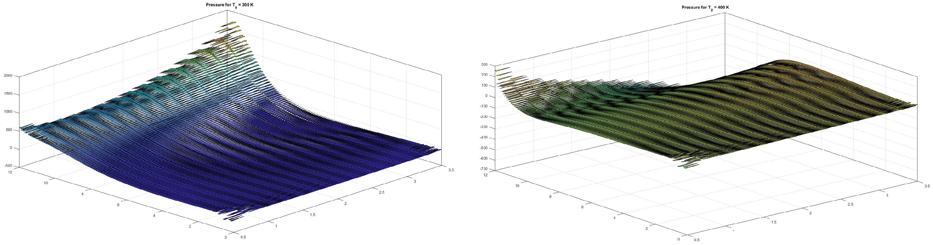
7.1. Pressure Dynamics When Changing the Temperature

In Figure 1 we present two numerical simulations that give the influence of an exterior known field of temperature on the blood pressure variations. They are in agreement with real-life examples: [16] says that high ambient temperatures are associated with lower blood pressure, more specifically the systolic blood pressure decreases with 5 mm Hg as the exterior medium temperature increases with 10 °C. Another article, Ref. [17], analyzes in more detail the variation in blood pressure with the variation in exterior temperature. So, when the exterior temperature is between 10 °C and 27 °C, the pressure decreases as the temperature increases, but if the temperature is higher than 27 °C, the pressure increases. Another study, Ref. [18], shows a significant influence of temperature in a closed space on blood pressure variation. As we can see in the figures below, if we increase the temperature (400 K), we obtain lower pressure values and if we decrease the temperature (300 K) we have higher pressure values.

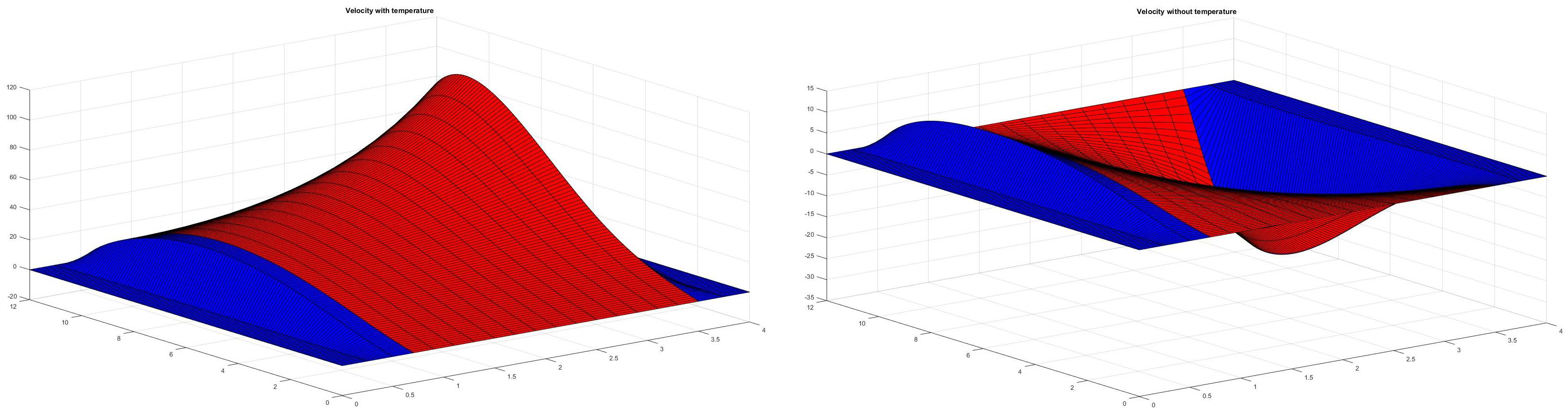
7.2. Temperature Influence on the Fluid–Structure Coupling

In real life, there are many situations in which the interaction between a fluid and an elastic medium is strongly influenced by temperature variations. As an example of the important role played by the temperature we mention the connection between the ambient temperature and the variation in velocity in these two articles [23,24]. In the simulations presented in Figure 2 it can be seen how the velocity profile has important differences if we take into account or not the temperature variations.

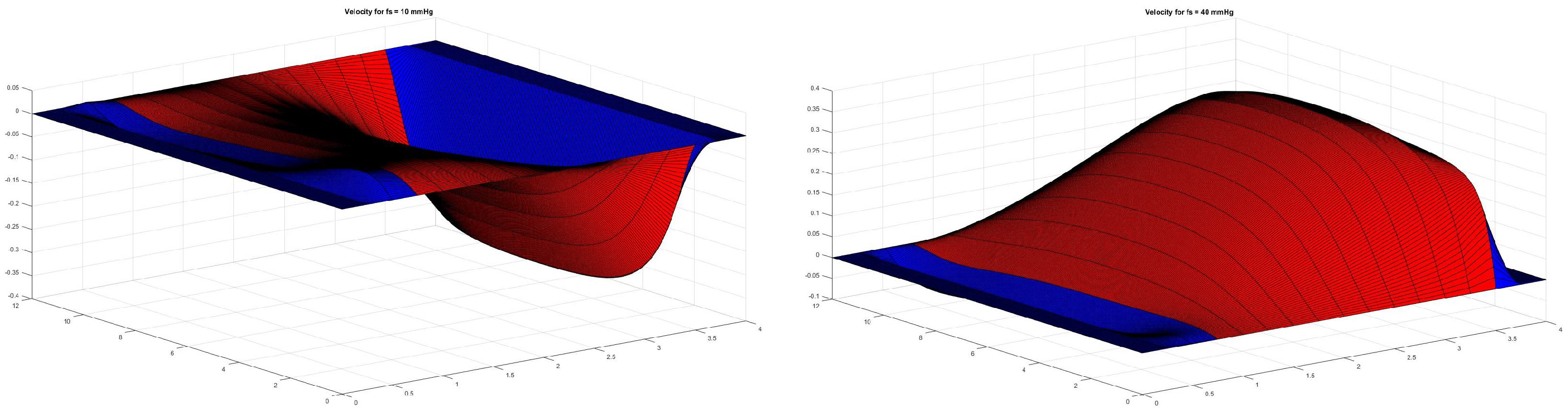
7.3. Velocity Dynamics When Changing the Forces

Among many other examples, the FSI model describes the interaction between the blood and the blood vessel walls. The blood flow through a leg vessel has an anti-gravity sense and this sense is modified when the vein loses its elasticity. When the vein has less elasticity, stagnation and recirculation of the blood might occur. The negative consequences of the lack of vein elasticity can be prevented by exterior compression applied on the blood vessel walls to diminish the blood recirculation phenomena. We have many examples that illustrate what we want to show in our study [25,26,27].

The compression forces act on the $x_1$-axis. As we will see in Figure 3, lower force values (10 mm Hg) lead to predominant negative values of the velocity and higher force (40 mm Hg) values to predominant positive values.

7.4. Convergence

Data used

Section 7.1 $dxs=0.25$, $dxf=0.2$, $dy=0.1$, $T_0=300K$, $T_1=300K$, ${\alpha }_f=303e^{-6}$, ${\alpha }_s=80e^{-6}$, $k_f=0.52$, $k_s=0.46$, $c_f=c_s=1$, ${\rho }_s={\rho }_0=1000$, $g=-9.81$, $\sigma =0.35$, $\tau =1$, $N=25$, $\epsilon =0.5$, ${\overrightarrow{f}}_s=1000$, $\rho =0.005$, $E=$1,000,000.

Section 7.2  $dxs=0.25$, $dxf=0.25$, $dy=0.05$, $T_0=300K$, $T_1=300K$, ${\alpha }_f=303e^{-6}$, ${\alpha }_s=80e^{-6}$, $k_f=0.52$, $k_s=0.46$, $\mu =0.003$, $c_f=3210$, $c_s=3617$, ${\rho }_s=960$, ${\rho }_0=900$, $g=-9.81$, $\sigma =0.3$, $\tau =1$, $N=400$, $\epsilon =0.5$, ${\overrightarrow{f}}_s=750,000$, $\rho =0.005$, $E=$500,000.

Section 7.3  $dxs=0.25$, $dxf=0.2$, $dy=0.1$, $T_0=300K$, $T_1=300K$, ${\alpha }_f=303e^{-6}$, ${\alpha }_s=80e^{-6}$, $k_f=0.52$, $k_s=0.46$, $c_f=c_s=1$, ${\rho }_s={\rho }_0=1000$, $g=-9.81$, $\sigma =0.35$, $\tau =1$, $N=25$, $\epsilon =0.5$, ${\overrightarrow{f}}_s=1000$, $\rho =0.005$, $E=$500,000.

The convergence has been reached in most cases for $N=4$, $N=5$. It can be said that the present numerical method has successfully demonstrated the applicability of the scheme in analyzing the fluid–structure interaction problem.

8. Conclusions

The present article represents the second part of a complete theoretical and numerical approach for an FSI problem when the temperature variations are also taken into account. The mathematical model describing this double-coupled problem (fluid/elastic medium/temperature variation) was introduced in [15] and it represents a challenging topic both from the mathematical and from the numerical viewpoints. In this article, we succeed in obtaining qualitative properties for the fluid pressure by means of variational techniques and proposing suitable approximation schemes, establishing stability and convergence results. Relying on these approximation schemes, we perform numerical simulations that show that our mathematical model faithfully describes real-life physical phenomena. We summarize step by step the proposed approximations, which establish the connection between the calculated solution and the exact solution of the problem. As the following scheme shows, we have proven the calculated solution converges by means of Uzawa’s algorithm to the solution of (123), solution equivalent to the solution of (117). This solution converges to the viscoelastic solution that converges to the exact solution when $\epsilon \to 0$.

$$\begin{array}{c}({\overrightarrow{\omega }}_{h,N}^{m,r},{\overrightarrow{u}}_{h,N}^{m,r},{\pi }_{h,N}^{m,r},S_{h,N}^{m,r})\\ \mathrm{solution}\mathrm{of}\left(123\right)\left(\mathrm{calculated}\mathrm{solution}\right)\end{array}{\displaystyle \underset{r\to \infty }{\overset{{\mathrm{Uzawa}}^{\prime }\mathrm{s}\mathrm{algorithm}}{\to }}}\begin{array}{c}({\overrightarrow{\omega }}_{h,N}^m,{\overrightarrow{u}}_{h,N}^m,{\pi }_{h,N}^m,S_{h,N}^m)\\ \mathrm{solution}\mathrm{of}\left(93\right)\end{array}$$

$$⟷\begin{array}{c}({\overrightarrow{\omega }}_{h,N},{\overrightarrow{u}}_{h,N},{\pi }_{h,N},S_{h,N})\\ \mathrm{solution}\mathrm{of}\left(117\right)\end{array}{\displaystyle \underset{N\to \infty }{\overset{h\to 0}{\to }}}\begin{array}{c}({\overrightarrow{\omega }}_{\epsilon },{\overrightarrow{u}}_{\epsilon },p_{\epsilon },S_{\epsilon })\\ \mathrm{solution}\mathrm{of}\left(72\right)\left(\mathrm{viscoelastic}\mathrm{solution}\right)\end{array}$$

$$\stackrel{\epsilon \to 0}{\to }\begin{array}{c}(\overrightarrow{\omega },\overrightarrow{u},p,S)\\ \mathrm{solution}\mathrm{of}\left(71\right)\left(\mathrm{exact}\mathrm{solution}\right)\end{array}$$

The novelty of this article is represented by the complex model considered since, as far as we know, there are no similar models in the literature (except for a simplified one in [14], in which the problems are decoupled so the study is much simpler) and the methods proposed for overcoming all the difficulties determined by the double-coupling, the nonlinearity and the nonhomogeneity of the problem. Since our work represents a mathematical and numerical study associated with a simplified model of blood flow through the circulatory system, some directions of future research could be to consider a more realistic geometry of the problem or a model closer to reality for modeling blood flow.

References

1. Grandmont, C.; Vergnet, F. Existence for a Quasi-Static Interaction Problem Between a Viscous Fluid and an Active Structure. J. Math. Fluid Mech. 2021, 23, 45. [Google Scholar] [CrossRef]
2. Bociu, L.; Čanić, S.; Muha, B.; Webster, J.T. Multilayered Poroelasticity Interacting with Stokes Flow. SIAM J. Math. Anal. 2021, 53, 6243–6279. [Google Scholar] [CrossRef]
3. Panasenko, G.P.; Stavre, R. Viscous Fluid–Thin Elastic Plate Interaction: Asymptotic Analysis with Respect to the Rigidity and Density of the Plate. Appl. Math. Optimiz. 2020, 81, 141–194. [Google Scholar] [CrossRef]
4. Panasenko, G.P.; Stavre, R. Three Dimensional Asymptotic Analysis of an Axisymmetric Flow in a Thin Tube with Thin Stiff Elastic Wall. J. Math. Fluid Mech. 2020, 22, 20. [Google Scholar] [CrossRef]
5. Stavre, R. Optimization of the blood pressure with the control in coefficients. Evol. Equ. Control. Theory 2020, 9, 131–151. [Google Scholar] [CrossRef]
6. Stavre, R. A boundary control problem for the blood flow in venous insufficiency. The general case. Nonlinear Anal. Real World Appl. 2016, 29, 98–116. [Google Scholar] [CrossRef]
7. Crosetto, P.; Reymond, P.; Deparis, S.; Kontaxakis, D.; Stergiopulos, N.; Quarteroni, A. Fluid–structure interaction simulation of aortic blood flow. Comput. Fluids 2011, 43, 46–57. [Google Scholar] [CrossRef]
8. Deparis, S.; Discacciati, M.; Fourestey, G.; Quarteroni, A. Fluid–structure algorithms based on Steklov–Poincaré operators. Comput. Methods Appl. Mech. Eng. 2006, 195, 5797–5812. [Google Scholar] [CrossRef]
9. Richter, T. Fluid-structure Interactions, Models, Analysis and Finite Elements. In Lecture Notes in Computational Science and Engineering; Barth, T.J., Griebel, M., Keyes, D.E., Nieminen, R.M., Roose, D., Schlick, T., Eds.; Springer: Berlin/Heidelberg, Germany, 2017; Volume 118. [Google Scholar] [CrossRef]
10. Diwate, M.; Tawade, J.V.; Janthe, P.G.; Garayev, M.; El-Meligy, M.; Kulkarni, N.; Gupta, M.; Khan, M.I. Numerical solutions for unsteady laminar boundary layer flow and heat transfer over a horizontal sheet with radiation and nonuniform heat Source/Sink. J. Radiat. Res. Appl. Sci. 2024, 17, 101196. [Google Scholar] [CrossRef]
11. Kulkarni, N.; Al-Dossari, M.; Tawade, J.; Alqahtani, A.; Khan, M.I.; Abdullaeva, B.; Waqas, M.; Khedher, N.B. Thermoelectric energy harvesting from geothermal micro-seepage. Int. J. Hydrogen Energy 2024, 93, 925–936. [Google Scholar] [CrossRef]
12. Maity, D.; Takahashi, T. Existence and uniqueness of strong solutions for the system of interaction between a compressible Navier-Stokes-Fourier fluid and a damped plate equation. Nonlinear Anal. Real World Appl. 2021, 59, 103267. [Google Scholar] [CrossRef]
13. Mácha, V.; Muha, B.; Šárka Nečasová, Š.; Roy, A.; Trifunović, S. Existence of a weak solution to a nonlinear fluid-structure interaction problem with heat exchange. Commun. Partial. Differ. Equ. 2022, 47, 1591–1635. [Google Scholar] [CrossRef]
14. Feppon, F.; Allaire, G.; Bordeu, F.; Cortial, J.; Dapegny, C. Shape optimization of a coupled thermal fluid-structure problem in a level set mesh evolution framework. Bol. Soc. Esp. Mat. Apl. 2019, 76, 413–458. [Google Scholar] [CrossRef]
15. Ciorogar, A.; Stavre, R. A Thermal Fluid–Structure Interaction Problem: Modeling, Variational and Numerical Analysis. J. Math. Fluid Mech. 2023, 25, 37. [Google Scholar] [CrossRef]
16. Kunutsor, S.K.; Powles, J.W. The effect of ambient temperature on blood pressure in a rural West African adult population: A cross-sectional study. Cardiovasc. J. Afr. 2010, 21, 17–20. [Google Scholar] [PubMed]
17. Xu, D.; Zhang, Y.; Wang, B.; Yang, H.; Ban, J.; Liu, F.; Li, T. Acute effects of temperature exposure on blood pressure: An hourly level panel study. Environ. Int. 2019, 124, 493–500. [Google Scholar] [CrossRef] [PubMed]
18. Hayashi, Y.; Ikaga, T.; Hoshi, T.; Ando, S. Effects of Indoor Air Temperature on Blood Pressure among Nursing Home Residents in Japan. In Proceedings of the 7th International Conference on Energy and Environment of Residential Buildings, Brisbane, Australia, 20–24 November 2016. [Google Scholar]
19. Carvalho, V.; Lopes, D.; Silva, J.; Puga, H.; Lima, R.A.; Teixeira, J.C.; Teixeira, S. Comparison of CFD and FSI simulations of blood flow in stenotic coronary arteries. In Applications of Computational Fluid Dynamics Simulation and Modeling; IntechOpen: London, UK, 2022. [Google Scholar] [CrossRef]
20. Temam, R. Navier-Stokes Equations; North-Holland: Amsterdam, The Netherlands, 1984. [Google Scholar]
21. Galdi, G.P. An Introduction to the Mathematical Theory of Navier–Stokes Equations; Springer-Verlag: New York, NY, USA, 1994. [Google Scholar]
22. Girault, V.; Raviart, P.A. Finite element approximation of the Navier-Stokes equations. In Lecture Notes in Mathematics; Dold, A., Eckmann, B., Eds.; Springer-Verlag: New York, NY, USA, 1979; 749p. [Google Scholar]
23. Abdalla, A.; Khanafer, K.; Vafai, K. Fluid-Structure Interactions in a Tissue During Hyperthermia. Numer. Heat Transf. Part Appl. 2014, 66, 1–6. [Google Scholar] [CrossRef]
24. Zhang, Z.; Yang, Z.; Nie, H.; Xu, L.; Yue, J.; Huang, Y. A thermal stress analysis of fluid–structure interaction applied to boiler water wall. Asia-Pac. J. Chem. Eng. 2020, 15, e2537. [Google Scholar] [CrossRef]
25. Baksamawi, H.A.; Mostapha, A.; Brill, A.; Vigolo, D.; Alexiadis, A. Modelling Particle Agglomeration on Through Elastic Valves Under Flow. ChemEngineering 2021, 5, 40. [Google Scholar] [CrossRef]
26. Gataulin, Y.A.; Yukhnev, A.D.; Rosukhovskiy, D.A. Fluid–structure interactions modeling the venous valve. J. Phys. Conf. Ser. 2018, 1128, 012009. [Google Scholar] [CrossRef]
27. Hajati, Z.; Moghanlou, F.S.; Vajdi, M.; Razavi, S.E.; Matin, S. Fluid-structure interaction of blood flow around a vein valve. Bioimpacts 2020, 10, 169–175. [Google Scholar] [CrossRef] [PubMed]
Figure 1. The pressure profiles for different exterior temperature values, T g = 300 K (left), T g = 400 K (right).
Axioms 14 00088 g001
Figure 2. The velocity with and without temperature.
Axioms 14 00088 g002
Figure 3. The velocity profiles for different force values, f s = 10 mm Hg (left), f s = 40 mm Hg (right).
Axioms 14 00088 g003
Disclaimer/Publisher’s Note: The statements, opinions and data contained in all publications are solely those of the individual author(s) and contributor(s) and not of MDPI and/or the editor(s). MDPI and/or the editor(s) disclaim responsibility for any injury to people or property resulting from any ideas, methods, instructions or products referred to in the content.