Convergence-Enhanced and ANN-Accelerated Solvers for Absolute Value Problems

Abstract

Absolute value problems of the form $Ax-\left|x\right|=b$, where $x\in {\mathbb{R}}^n$ is the unknown vector, $b\in {\mathbb{R}}^n$ is a given vector, and $A\in {\mathbb{R}}^{n\times n}$ is a matrix, arise in a wide range of scientific and engineering applications. Their solution is challenging due to the non-differentiability of the absolute value operator and the possible existence of multiple solutions. Classical iterative techniques often suffer from slow convergence, strong sensitivity to the choice of initial vectors, and limited global convergence guarantees. In this study, we introduce a novel two-step iterative scheme that incorporates an adaptive initialization strategy enhanced by artificial neural networks (ANNs). The proposed method attains global linear convergence and local third-order convergence, thereby combining robustness with high accuracy. Numerical experiments on a range of benchmark problems—including cases with both unique and multiple solutions—demonstrate that the ANN-assisted initialization substantially accelerates convergence. In particular, it reduces the number of iterations, computational time, and residual errors across multiple norms, including both the Euclidean and infinity norms. These findings demonstrate that coupling a high-order two-step solver with ANN-based adaptive initialization yields a reliable and efficient framework for solving absolute value problems in both theoretical analysis and practical large-scale applications.

1. Introduction

Absolute Value Equations (AVEs) of the form

$$Ax-\left|x\right|=b,A\in {\mathbb{R}}^{n\times n},x,b\in {\mathbb{R}}^n,$$

(1)

where $\left|x\right|$ denotes the componentwise absolute value of x, have emerged as a central class of problems in applied mathematics, computer science, and engineering. AVEs unify several nonlinear structures and are closely related to linear complementarity problems (LCPs), variational inequalities (VIs), piecewise-linear systems, and various optimization models [1,2]. Their study has attracted considerable attention both for their wide range of applications and for the mathematical challenges posed by their inherent nonsmoothness.

The significance of AVEs lies in their ability to model diverse real-world phenomena across different disciplines. In operations research, they arise as reformulations of optimization problems with complementarity constraints  [3]. In control theory, they represent switching systems and piecewise-linear controllers [4]. In structural engineering and mechanics, they naturally capture contact problems and frictional forces, with the absolute value function modeling transitions between compression and tension. In biomedical engineering, AVEs describe threshold-driven dynamics such as glucose–insulin regulation, cardiac electrophysiology, and biomechanical load–response systems [5,6]. In computer science and machine learning, they appear in sparsity-inducing regularizations, signal recovery, and robust regression models [7]. Because of this breadth, efficient solution methods for AVEs are not only of mathematical interest but also crucial for handling larger systems where absolute value operators introduce discontinuities and nonsmooth behavior.

Early approaches to solving AVEs were based on exact transformations, but they suffer from several fundamental limitations. The piecewise-linear structure of the absolute value function allows reformulation into up to $2^n$ linear systems [8], yet this quickly becomes infeasible as n increases. Reformulations into linear complementarity problems (LCPs) and variational inequalities (VIs) [9] permit the use of established algorithms but at the cost of increased dimensionality and complexity. Symbolic and perturbation methods [10] provide valuable theoretical insight into existence, uniqueness, and sensitivity, but they do not scale to large systems. Overall, these approaches are limited in their applicability to high-dimensional or sparse problems and offer little practical utility for real-world computations.

Because of these drawbacks, iterative solvers have become indispensable. Methods such as semi-smooth Newton approaches [11,12], SOR schemes [13], and projection algorithms [14] are widely used for their scalability, simplicity, and ability to exploit sparsity in large-scale AVEs. For engineering problems with tens of thousands of variables, iterative methods are often the only viable option, owing to their adaptability and parallelizability [15]. Many existing iterative schemes stem from quadrature-based integral reformulations [16], but these approaches suffer from well-known drawbacks:

• Stability: Quadrature-based schemes are highly sensitive to discretization parameters, often leading to unstable convergence.
• Convergence Rate: Most quadrature-derived methods achieve at best linear or quadratic convergence [17].
• Robustness: Their performance depends on accurate numerical integration, which becomes problematic for the nonsmooth functions inherent in AVEs.
• Computational Cost: In multidimensional problems, quadrature rules require evaluating a large number of integrand points, leading to significant overhead.

These limitations underscore the necessity of developing iterative methods that avoid reliance on quadrature rules and instead exploit the intrinsic algebraic and numerical properties of AVEs. Over the past two decades, research in this direction has accelerated considerably. Rohn [18] and Mangasarian [19] established foundational existence and uniqueness results, which motivated the development of semi-smooth Newton methods, while projection and splitting strategies such as Picard iteration and successive approximation schemes have also been studied extensively [20,21]. More recent research has focused on enhancements including preconditioning [22], extrapolation techniques [23], adaptive step strategies [24], and acceleration via artificial neural networks (ANNs) [25]. Nevertheless, most existing methods remain constrained by low convergence order, stability concerns, and the absence of global convergence guarantees, while ANN-based hybridizations are still in an early stage of development.

Despite the breadth of existing techniques, a closer examination reveals several unresolved limitations that motivate the present work. Classical iterative strategies for AVEs—including semi-smooth Newton methods [26], projection–splitting techniques [27], and quadrature-based updates [28]—often exhibit either a low order of convergence or a strong sensitivity to the nonsmooth regions of the solution space. When absolute-value nonlinearities induce switching, discontinuities, or ill-conditioning, even methods with higher local convergence rates typically depend on structural assumptions that restrict their robustness. Recent ANN-based enhancements [29] improve the prediction of descent directions or step sizes, yet such hybrid approaches seldom integrate the network output directly into the algebraic structure of the update, limiting both their stability and theoretical guarantees. These gaps highlight the need for algorithms that (i) retain the simplicity and low computational cost of classical two-step schemes, (ii) achieve higher practical efficiency without compromising stability, and (iii) incorporate ANN-generated corrections in a mathematically controlled manner. Motivated by these challenges, we modify an existing locally third-order two-step method and embed an ANN-driven correction term into its iterative map, producing a hybrid scheme that improves global behavior while preserving provable local convergence properties [30].

In this work, we refine a classical two-step method for AVEs that possesses local third-order and global linear convergence, with the aim of improving its stability and enlarging its region of convergence. We further introduce a hybrid ANN strategy in which network-predicted correction terms are embedded directly into the update, thereby accelerating convergence without altering the method’s underlying theoretical framework. Both the local analysis and extensive numerical experiments indicate that the ANN-enhanced scheme achieves higher efficiency, greater robustness with respect to difficult initial guesses, and superior performance on large-scale and nonsmooth AVEs.

1.1. Main Contributions

The main contributions of this paper can be summarized as follows:

• A two-step iterative method is developed, achieving global linear convergence and local quartic convergence.
• Integration of ANN-based acceleration.
• A comprehensive computational analysis evaluating convergence behavior, runtime efficiency, and memory utilization.
• Extensive numerical validation is carried out on benchmark AVEs, large-scale systems, initial/boundary value AVEs, and biomechanical applications.
• A conceptual bridge is established between deterministic iterative theory and AI-based accelerators.

1.2. Structure of the Paper

• Section 2: Construction of the proposed scheme and analysis of its convergence properties.
• Section 3: Numerical methodology, implementation details, and ANN-based acceleration strategy.
• Section 4: Numerical results for four categories:
  • benchmark AVEs,
  • large-scale systems,
  • initial and boundary value AVEs,
  • biomechanical applications.
• Section 5: Conclusions and future research directions.

2. Construction and Convergence Analysis of the Proposed Scheme

We introduce the notation and background required for the analysis of AVEs. Let e denote a unit vector and I the identity matrix of appropriate dimension. The Euclidean norm of a vector x is defined as $\parallel x\parallel =\sqrt{x^{T}x}$. The function $\mathrm{sign}\left(x\right)$ represents a vector whose components take the values 1, 0, or $-1$ depending on whether the corresponding entry of x is positive, zero, or negative, respectively. Furthermore, $\mathrm{diag}\left(\mathrm{sign}\right(x\left)\right)$ denotes the diagonal matrix with the components of $\mathrm{sign}\left(x\right)$ on its diagonal. A generalized Jacobian of the absolute value function $\left|x\right|$ at x can then be expressed as $D\left(x\right)=\mathrm{diag}\left(\mathrm{sign}\right(x\left)\right)$.

Based on these definitions, we consider the nonlinear function

$$f\left(x\right)=Ax-\left|x\right|-b,$$

(2)

where $A\in {\mathbb{R}}^{n\times n}$ and $b\in {\mathbb{R}}^n$. The generalized Jacobian of $f\left(x\right)$ at x is given by

$$f^{\prime }\left(x\right)=A-D\left(x\right),D\left(x\right)=\mathrm{diag}\left(\mathrm{sign}\left(x\right)\right).$$

(3)

To solve absolute value equations (AVEs) of the form $Ax-\left|x\right|=b$, the classical generalized Newton-type iteration is commonly employed [31]:

$$x^{[k+1]}={\left(A-D\left(x^{\left[k\right]}\right)\right)}^{-1}b,k=0,1,2,\dots ,$$

(4)

where $D\left(x^{\left[k\right]}\right)=\mathrm{diag}\left(\mathrm{sign}\left(x^{\left[k\right]}\right)\right)$. This iteration serves as the foundation for several higher-order and accelerated schemes.

A higher-order variant, based on a two-step Trube-type method [32], is defined as

$$\left\{\begin{array}{c}{y}^{\left[k\right]}=x^{\left[k\right]}-{\left(A-D\left(x^{\left[k\right]}\right)\right)}^{-1}f\left(x^{\left[k\right]}\right),\hfill \\ x^{[k+1]}=x^{\left[k\right]}-{\left(A-D\left(x^{\left[k\right]}\right)\right)}^{-1}\left(f\left(y^{\left[k\right]}\right)+f\left(x^{\left[k\right]}\right)\right),\hfill \end{array}\right.$$

(5)

where $f\left(x\right)=Ax-\left|x\right|-b$. This two-step scheme achieves global linear convergence and local quadratic convergence, requiring at each iteration the solution of two linear systems and one LU factorization (or Jacobian evaluation). We refer to this method as TAV.

Another two-step method was proposed in ref. [33], formulated as

$$\left\{\begin{array}{c}{y}^{\left[k\right]}=x^{\left[k\right]}-{\left(A-D\left(x^{\left[k\right]}\right)\right)}^{-1}f\left(x^{\left[k\right]}\right),\hfill \\ x^{[k+1]}=y^{\left[k\right]}-{\left(A-D\left(x^{\left[k\right]}\right)\right)}^{-1}f\left(y^{\left[k\right]}\right),\hfill \end{array}\right.$$

(6)

which attains global linear and local quadratic convergence with computational requirements similar to the previous scheme.

In addition, predictor–corrector strategies employing quadrature-based acceleration have been proposed. For instance, Khan et al. [34] combine the classical Newton predictor with Simpson’s rule as a corrector:

$$\left\{\begin{array}{c}{y}^{\left[k\right]}=x^{\left[k\right]}-{\left(A-D\left(x^{\left[k\right]}\right)\right)}^{-1}f\left(x^{\left[k\right]}\right),\hfill \\ x^{[k+1]}=x^{\left[k\right]}-6{\left(f^{\prime \left[k\right]}+4f^{\prime }\left({\displaystyle \frac{x^{\left[k\right]}+y^{\left[k\right]}}{2}}\right)+f^{\prime \left[k\right]}\right)}^{-1}f\left(x^{\left[k\right]}\right),\hfill \end{array}\right.$$

(7)

which achieves global linear and local quadratic convergence. This method, abbreviated as AEV, requires one nonlinear function evaluation and three Jacobian or LU factorizations per iteration.

Similarly, Rahpeymaii et al. [35] employ the Simpson 3/8 rule:

$$\left\{\begin{array}{c}{y}^{\left[k\right]}=x^{\left[k\right]}-{\left(A-D\left(x^{\left[k\right]}\right)\right)}^{-1}f\left(x^{\left[k\right]}\right),\hfill \\ x^{[k+1]}=x^{\left[k\right]}-8{\left(f^{\prime \left[k\right]}+3f^{\prime }\left({\displaystyle \frac{2x^{\left[k\right]}+y^{\left[k\right]}}{3}}\right)+3f^{\prime }\left({\displaystyle \frac{x^{\left[k\right]}+2y^{\left[k\right]}}{3}}\right)+f^{\prime \left[k\right]}\right)}^{-1}f\left(x^{\left[k\right]}\right),\hfill \end{array}\right.$$

(8)

which likewise achieves global linear and local quadratic convergence. Each iteration requires two linear system solves and four Jacobian evaluations or LU factorizations, and we denote this method by HAV.

Finally, a three-step method [36] is given by

$$\left\{\begin{array}{c}{y}^{\left[k\right]}=x^{\left[k\right]}-{\left(A-D\left(x^{\left[k\right]}\right)\right)}^{-1}f\left(x^{\left[k\right]}\right),\hfill \\ z^{\left[k\right]}=y^{\left[k\right]}-{\displaystyle \frac{{\left(A-D\left(x^{\left[k\right]}\right)\right)}^{-1}+{\left(A-D\left(y^{\left[k\right]}\right)\right)}^{-1}}{2}}f\left(y^{\left[k\right]}\right),\hfill \\ x^{[k+1]}=z^{\left[k\right]}-{\left(A-D\left(z^{\left[k\right]}\right)\right)}^{-1}f\left(z^{\left[k\right]}\right),\hfill \end{array}\right.$$

(9)

which attains global linear and local quadratic convergence, with two linear system solves and three Jacobian/LU factorizations per iteration. We denote this scheme by FAV.

2.1. Development and Analysis of Numerical Schemes for Solving AVEs

We build on the third-order method proposed in [37] for solving nonlinear equations, which is defined by

$$\left\{\begin{array}{c}{y}^{\left[k\right]}=x^{\left[k\right]}-{\displaystyle \frac{f\left(x^{\left[k\right]}\right)}{f^{\prime }\left(x^{\left[k\right]}\right)}},\hfill \\ x^{[k+1]}=x^{\left[k\right]}-{\displaystyle \frac{2f\left(y^{\left[k\right]}\right)}{3f^{\prime }\left(y^{\left[k\right]}\right)-f^{\prime }\left(x^{\left[k\right]}\right)}}{\displaystyle \frac{f\left(x^{\left[k\right]}\right)}{f^{\prime }\left(x^{\left[k\right]}\right)}}.\hfill \end{array}\right.$$

(10)

where the errors are given by $e^{\left[k\right]}=x^{\left[k\right]}-\xi$ and $e^{[k+1]}=x^{[k+1]}-\xi$. The associated local error equation is

$$e^{[k+1]}=\frac{1}{2}\left(-2d_2^2+d_3\right){\left(e^{\left[k\right]}\right)}^3+\mathcal{O}\left({\left(e^{\left[k\right]}\right)}^4\right),d_j={\displaystyle \frac{f^{\left(j\right)}\left(\xi \right)}{j!f^{\prime }\left(\xi \right)}},j\ge 2.$$

To extend this approach to absolute value equations (AVEs), the method is generalized to the following form, referred to as the SMV method:

$$\left\{\begin{array}{cc}\hfill y^{\left[k\right]}& =x^{\left[k\right]}-{(A-D\left(x^{\left[k\right]}\right))}^{-1}f\left(x^{\left[k\right]}\right),\hfill \\ \hfill x^{[k+1]}& =x^{\left[k\right]}-{\displaystyle \frac{2f\left(y^{\left[k\right]}\right)}{3f^{\prime }\left(y^{\left[k\right]}\right)-f^{\prime }\left(x^{\left[k\right]}\right)}}{\displaystyle \frac{f\left(x^{\left[k\right]}\right)}{f^{\prime }\left(x^{\left[k\right]}\right)}}.\hfill \end{array}\right.$$

(11)

2.1.1. Convergence Analysis

We present a rigorous convergence analysis of the proposed iterative method. First, we show that each iteration is well defined; next, we establish the boundedness of the generated sequence; finally, we prove the main convergence theorem.

Well-Definedness of the Scheme

We recall that the generalized Newton method (Lemma 2, [38]) can be employed as a predictor step:

$$y^{\left[k\right]}=x^{\left[k\right]}-{\left(A-D\left(x^{\left[k\right]}\right)\right)}^{-1}f\left(x^{\left[k\right]}\right).$$

(12)

Based on (12), the proposed scheme is written as

$$x^{[k+1]}=x^{\left[k\right]}-2f^{\prime }\left(y^{\left[k\right]}\right)M_2^{-1}{u}^{\left[k\right]},$$

(13)

where

$$M_2=3f^{\prime }\left(y^{\left[k\right]}\right)-f^{\prime }\left(x^{\left[k\right]}\right),u^{\left[k\right]}={\displaystyle \frac{f\left(x^{\left[k\right]}\right)}{f^{\prime }\left(x^{\left[k\right]}\right)}}.$$

To ensure that the sequence $\left\{x^{\left[k\right]}\right\}$ is well defined, we observe that the predictor step (12) is already established as bounded (see ref. [39]). It therefore remains to verify the nonsingularity of

$$\begin{array}{ccc}\hfill 3f^{\prime }\left(y^{\left[k\right]}\right)-f^{\prime }\left(x^{\left[k\right]}\right)& =& 3A-3D\left(y^{\left[k\right]}\right)-A+D\left(x^{\left[k\right]}\right)\hfill \\ & =& 2A-3D\left(y^{\left[k\right]}\right)+D\left(x^{\left[k\right]}\right).\hfill \end{array}$$

(14)

Lemma 1. 

If the singular values of $A\in {\mathbb{R}}^{n\times n}$ satisfy ${\sigma }_{min}\left(A\right)>1$, then the diagonal matrix

$${\left(2A-3D\left(y^{\left[k\right]}\right)+D\left(x^{\left[k\right]}\right)\right)}^{-1}$$

exists for all diagonal matrices $D\left(x^{\left[k\right]}\right)$, $D\left(y^{\left[k\right]}\right)$ with entries in $\{-1,0,1\}$.

Proof. 

Assume, for contradiction, that $M_2$ is singular. Then there exists a nonzero vector $v\ne 0$ such that

$$M_{2}v=0.$$

(15)

Taking norms, we obtain

$$\begin{array}{ccc}\hfill v^{T}v& <& v^T{A}^{T}Av\hfill \\ & <& v^T{\left(2A-3D\left(y^{\left[k\right]}\right)+D\left(x^{\left[k\right]}\right)\right)}^T\left(2A-3D\left(y^{\left[k\right]}\right)+D\left(x^{\left[k\right]}\right)\right)v.\hfill \end{array}$$

(16)

Expanding the diagonal contributions gives

$$v^T{A}^{T}Av=v^T\left(4A^{T}A+9D\left(y^{\left[k\right]}\right)D\left(y^{\left[k\right]}\right)+D\left(x^{\left[k\right]}\right)D\left(x^{\left[k\right]}\right)+\mathrm{cross}\mathrm{terms}\right)v.$$

(17)

Since for any diagonal matrix with entries in $\{-1,0,1\}$ it holds that $\parallel D(·)\parallel \le 1$, we deduce

$$v^T{A}^{T}Av\ge 4v^{T}v.$$

(18)

This yields the contradiction

$$v^{T}v<\frac{1}{4}{v}^T{A}^{T}Av<v^{T}v,$$

(19)

which is impossible whenever ${\sigma }_{min}\left(A\right)>1$. Therefore, $M_2$ is nonsingular.    □

2.2. Boundedness of the Sequence

We now establish the boundedness of the sequence $\left\{x^{\left[k\right]}\right\}$. The corrector step can be expressed as

$$x^{[k+1]}=x^{\left[k\right]}-2f^{\prime }\left(y^{\left[k\right]}\right){\left(3f^{\prime }\left(y^{\left[k\right]}\right)-f^{\prime }\left(x^{\left[k\right]}\right)\right)}^{-1}{u}^{\left[k\right]},$$

(20)

or, equivalently,

$$x^{[k+1]}=x^{\left[k\right]}-N^{\left[k\right]}{\left(M_2\right)}^{-1}f\left(x^{\left[k\right]}\right),$$

(21)

where

$$N^{\left[k\right]}={\displaystyle \frac{2f^{\prime }\left(y^{\left[k\right]}\right)}{f^{\prime }\left(x^{\left[k\right]}\right)}}.$$

Hence,

$$\begin{array}{ccc}\hfill M_2{x}^{[k+1]}& =& M_2{x}^{\left[k\right]}-N^{\left[k\right]}f\left(x^{\left[k\right]}\right)\hfill \\ & =& M_2\left(2A-3D\left(y^{\left[k\right]}\right)+D\left(x^{\left[k\right]}\right)\right)-N^{\left[k\right]}\left(A{x}^{\left[k\right]}-\left|x^{\left[k\right]}\right|-b\right).\hfill \end{array}$$

The right-hand side is a linear combination of $x^{\left[k\right]}$, b, and the diagonal matrices $D\left(x^{\left[k\right]}\right)$ and $D\left(y^{\left[k\right]}\right)$. Since the entries of these diagonal matrices are bounded in absolute value by 1, it follows that the sequence $\left\{x^{\left[k\right]}\right\}$ remains bounded (see Proposition 3 in ref. [40]).

2.3. Main Convergence Result

We now present the principal convergence theorem.

Theorem 1. 

  If

$$∥2A-3D\left(y^{\left[k\right]}\right)+D\left(x^{\left[k\right]}\right)∥<\frac{1}{4},$$

(22)

for any diagonal matrix with entries from $\{-1,0,1\}$, then the sequence generated by the scheme converges to the solution ζ of the AVE.

Proof. 

Let $e^{\left[k\right]}=x^{\left[k\right]}-\zeta$ denote the error at the kth iteration, where $\zeta$ is the exact solution of the AVE. Since $\zeta$ satisfies

$$\begin{array}{ccc}\hfill f\left(\zeta \right)& =& A\zeta -\left|\zeta \right|-b\hfill \\ & =& 0,\hfill \end{array}$$

(23)

we can express the iteration error as

$$x^{[k+1]}-\zeta =x^{\left[k\right]}-\zeta -N_1^{\left[k\right]}{M}_2^{-1}{u}^{\left[k\right]}.$$

(24)

Multiplying both sides by $M_2$ yields

$$M_2(x^{[k+1]}-\zeta )=M_2(x^{\left[k\right]}-\zeta )-N_1^{\left[k\right]}f\left(x^{\left[k\right]}\right).$$

(25)

By definition of the scheme, we obtain

$$\begin{array}{ccc}\hfill M_2(x^{[k+1]}-\zeta )& =& M_2(x^{\left[k\right]}-\zeta )-2N_1^{\left[k\right]}f\left(x^{\left[k\right]}\right)+2N_1^{\left[k\right]}f\left(\zeta \right)\hfill \\ & =& M_2(x^{\left[k\right]}-\zeta )-2N_1^{\left[k\right]}\left(f\left(x^{\left[k\right]}\right)-f\left(\zeta \right)\right)\hfill \\ & =& M_2(x^{\left[k\right]}-\zeta )-2N_1^{\left[k\right]}\left(A(x^{\left[k\right]}-\zeta )-\left(\right|x^{\left[k\right]}|-|\zeta \left|\right)\right)\hfill \\ & =& M_2(x^{\left[k\right]}-\zeta )-2N_1^{\left[k\right]}A(x^{\left[k\right]}-\zeta )+2N_1^{\left[k\right]}\left(\right|x^{\left[k\right]}|-|\zeta \left|\right)\hfill \\ & \le & (M_2-2A)(x^{\left[k\right]}-\zeta )+2\left(\right|x^{\left[k\right]}|-|\zeta \left|\right)\hfill \\ & =& \left(-3D\left(y^{\left[k\right]}\right)+D\left(x^{\left[k\right]}\right)\right)(x^{\left[k\right]}-\zeta )+2\left(\right|x^{\left[k\right]}|-|\zeta \left|\right).\hfill \end{array}$$

(26)

Therefore, the error satisfies

$$x^{[k+1]}-\zeta \le M_2^{-1}\left[2\left(\right|x^{\left[k\right]}|-|\zeta \left|\right)+\left(-3D\left(y^{\left[k\right]}\right)+D\left(x^{\left[k\right]}\right)\right)(x^{\left[k\right]}-\zeta )\right].$$

(27)

Introducing $h^{[*]}=-3D\left(y^{\left[k\right]}\right)+D\left(x^{\left[k\right]}\right)$, this inequality becomes

$$x^{[k+1]}-\zeta \le M_2^{-1}\left[2\left(\right|x^{\left[k\right]}|-|\zeta \left|\right)+h^{[*]}(x^{\left[k\right]}-\zeta )\right].$$

(28)

Taking norms on both sides and using the Lipschitz continuity of the absolute value function (see Lemma 5 in ref. [41]), we obtain

$$\parallel |x^{\left[k\right]}|-|\zeta |\parallel \le 2\parallel x^{\left[k\right]}-\zeta \parallel .$$

(29)

Consequently,

$$\parallel x^{[k+1]}-\zeta \parallel \le \parallel M_2^{-1}\parallel \left(4\parallel x^{\left[k\right]}-\zeta \parallel +\parallel h^{[*]}\parallel \parallel x^{\left[k\right]}-\zeta \parallel \right).$$

(30)

Since both $D\left(x^{\left[k\right]}\right)$ and $D\left(y^{\left[k\right]}\right)$ are diagonal matrices, it follows that

$$\begin{array}{ccc}\hfill \parallel h^{[*]}\parallel & =& \parallel -3D\left(y^{\left[k\right]}\right)+D\left(x^{\left[k\right]}\right)\parallel \hfill \\ & \le & 3\parallel D\left(y^{\left[k\right]}\right)\parallel +\parallel D\left(x^{\left[k\right]}\right)\parallel \le 2.\hfill \end{array}$$

(31)

Combining (30) and (31), we obtain

$$\parallel x^{[k+1]}-\zeta \parallel \le 4\parallel M_2^{-1}\parallel \parallel x^{\left[k\right]}-\zeta \parallel < \parallel x^{\left[k\right]}-\zeta \parallel .$$

(32)

Finally, since $\parallel M_2^{-1}\parallel <\frac{1}{4}$, it follows that the iterative scheme produces a globally linearly convergent sequence.    □

2.4. Unique Solvability

Lemma 2. 

Let $\parallel A^{-1}\parallel <\frac{1}{5}$ and $\parallel 3D\left(y^{\left[k\right]}\right)\parallel ,\parallel D\left(x^{\left[k\right]}\right)\parallel \ne 0$. Then the AVE admits a unique solution for any b, and the proposed method is well defined and convergent for every initial vector $x^{\left[0\right]}$.

Proof. 

The unique solvability of the AVE for any right-hand side b requires that

$$\parallel A^{-1}\parallel <1.$$

(33)

Since $A^{-1}$ exists and, in addition, the inequality

$$\parallel 2A^{-1}\parallel \parallel 3D\left(y^{\left[k\right]}\right)-D\left(x^{\left[k\right]}\right)\parallel <1$$

(34)

holds, we can apply the Banach perturbation lemma [42].

From this lemma, it follows that

$$\begin{array}{ccc}\hfill \parallel {\left(3D\left(y^{\left[k\right]}\right)-D\left(x^{\left[k\right]}\right)\right)}^{-1}\parallel & =& \parallel {\left(2A-3D\left(y^{\left[k\right]}\right)+D\left(x^{\left[k\right]}\right)\right)}^{-1}\parallel \hfill \\ & \le & {\displaystyle \frac{{\parallel \left(2A\right)}^{-1}\parallel \parallel 3D\left(y^{\left[k\right]}\right)-D\left(x^{\left[k\right]}\right)\parallel }{{1-\parallel \left(2A\right)}^{-1}\parallel \parallel 3D\left(y^{\left[k\right]}\right)-D\left(x^{\left[k\right]}\right)\parallel }}.\hfill \end{array}$$

(35)

Using ${\parallel \left(2A\right)}^{-1}\parallel =\frac{1}{2}\parallel A^{-1}\parallel$ and the assumption $\parallel A^{-1}\parallel <\frac{1}{5}$, we obtain

$$\begin{array}{ccc}\hfill \parallel {\left(3D\left(y^{\left[k\right]}\right)-D\left(x^{\left[k\right]}\right)\right)}^{-1}\parallel & \le & {\displaystyle \frac{\frac{1}{2}\parallel A^{-1}\parallel ·2}{1-\frac{1}{2}\parallel A^{-1}\parallel ·2}}\hfill \\ & \le & {\displaystyle \frac{\frac{1}{5}}{1-\frac{1}{5}}}\hfill \\ & <& \frac{1}{4}.\hfill \end{array}$$

(36)

Therefore, the matrix ${\left(2A-3D\left(y^{\left[k\right]}\right)+D\left(x^{\left[k\right]}\right)\right)}^{-1}$ is bounded by $\frac{1}{4}$. By Theorem  1, this bound guarantees that the proposed scheme converges linearly to the unique solution of (1).    □

Remark 1. 

The assumptions $\parallel A^{-1}\parallel <\frac{1}{5}$ and $\parallel M_2^{-1}\parallel <\frac{1}{4}$ are introduced solely as sufficient conditions for verifying the hypotheses of the Banach perturbation lemma (invertibility and contractivity), thereby ensuring uniqueness and convergence within the theoretical analysis. These bounds, however, are not necessary. As illustrated by the numerical results (

Table 1. Comparison of iterative approximations and residual errors for the schemes TAV, AEV, FAV, HAV, and SMV applied to $f\left(x\right)$ in Example 1.

Scheme	${\mathit{X}}_1$	${\mathit{X}}_2$	${\mathit{X}}_3$	${\mathit{X}}_4$	Residual Error
TAV	$\begin{array}{c}{x}^{\left[1\right]}=1.043\\ x^{\left[2\right]}=1.0702\\ x^{\left[3\right]}=1.070820\end{array}$	$\begin{array}{c}{x}^{\left[1\right]}=0.98\\ x^{\left[2\right]}=0.980\\ x^{\left[3\right]}=0.98006382\end{array}$	$\begin{array}{c}{x}^{\left[1\right]}=1.0543\\ x^{\left[2\right]}=1.056242\\ x^{\left[3\right]}=1.056277454\end{array}$	$\begin{array}{c}{x}^{\left[1\right]}=1.0722\\ x^{\left[2\right]}=1.0708263\\ x^{\left[3\right]}=1.07082034\end{array}$	$\begin{array}{c}4.3\times {10}^{-1}\\ 6.7\times {10}^{-7}\\ 9.1\times {10}^{-16}\end{array}$
AEV	$\begin{array}{c}{x}^{\left[1\right]}=1.045\\ x^{\left[2\right]}=1.07023\\ x^{\left[3\right]}=1.070820\end{array}$	$\begin{array}{c}{x}^{\left[1\right]}=0.98\\ x^{\left[2\right]}=0.980\\ x^{\left[3\right]}=0.98006382\end{array}$	$\begin{array}{c}{x}^{\left[1\right]}=1.0564\\ x^{\left[2\right]}=1.056234\\ x^{\left[3\right]}=1.056277454\end{array}$	$\begin{array}{c}{x}^{\left[1\right]}=1.0734\\ x^{\left[2\right]}=1.0708266\\ x^{\left[3\right]}=1.07082034\end{array}$	$\begin{array}{c}1.24\times {10}^{-1}\\ 5.63\times {10}^{-04}\\ 3.73\times {10}^{-13}\end{array}$
FAV	$\begin{array}{c}{x}^{\left[1\right]}=1.044\\ x^{\left[2\right]}=1.07075\\ x^{\left[3\right]}=1.070820\end{array}$	$\begin{array}{c}{x}^{\left[1\right]}=0.98\\ x^{\left[2\right]}=0.980\\ x^{\left[3\right]}=0.98006382\end{array}$	$\begin{array}{c}{x}^{\left[1\right]}=1.0575\\ x^{\left[2\right]}=1.056234\\ x^{\left[3\right]}=1.056277454\end{array}$	$\begin{array}{c}{x}^{\left[1\right]}=1.0743\\ x^{\left[2\right]}=1.0708244\\ x^{\left[3\right]}=1.07082034\end{array}$	$$\begin{gathered} 1.25\times {10}^{-2} \\ 0.53\times {10}^{-09} \\ 0.34\times {10}^{-20 †} \end{gathered}$$
HAV	$\begin{array}{c}{x}^{\left[1\right]}=1.0447\\ x^{\left[2\right]}=1.070344\\ x^{\left[3\right]}=1.070820\end{array}$	$\begin{array}{c}{x}^{\left[1\right]}=0.9834\\ x^{\left[2\right]}=0.980834\\ x^{\left[3\right]}=0.98006382\end{array}$	$\begin{array}{c}{x}^{\left[1\right]}=0.981\\ x^{\left[2\right]}=0.98063\\ x^{\left[3\right]}=0.98006382\end{array}$	$\begin{array}{c}{x}^{\left[1\right]}=1.0734\\ x^{\left[2\right]}=1.070826\\ x^{\left[3\right]}=1.07082034\end{array}$	1.25 × 10−1 0.76 × 10−7 0.35 × 10−19 †
SMV	$\begin{array}{c}{x}^{\left[1\right]}=1.0447\\ x^{\left[2\right]}=1.070344\\ x^{\left[3\right]}=1.070820\end{array}$	$\begin{array}{c}{x}^{\left[1\right]}=0.9853\\ x^{\left[2\right]}=0.98046\\ x^{\left[3\right]}=0.98006382\end{array}$	$\begin{array}{c}{x}^{\left[1\right]}=0.9843\\ x^{\left[2\right]}=0.980447\\ x^{\left[3\right]}=0.98006382\end{array}$	$\begin{array}{c}{x}^{\left[1\right]}=1.074\\ x^{\left[2\right]}=1.070826\\ x^{\left[3\right]}=1.07082034\end{array}$	1.29 × 10−4 0.08 × 10−18 † 0.10 × 10−27 †

^† All computations were performed using MATLAB variable precision arithmetic (VPA) with digits = 64, employing a numerical tolerance of ${10}^{-30}$.

,

Table 2. Performance of the ANN-accelerated SMV scheme (SMV-AN) applied to Example 1, reporting iterations, mean squared error (MSE), CPU time, memory usage, gradient magnitude, and adaptive parameter $\mu$.

Scheme	Epoch	MSE	CPU Time	Memory (Kb)	Gradient	$\mathit{\mu }$
SMV-AN	200	$4.178\times {10}^{-5}$	3.4354	23,048	$1.23\times {10}^{-7}$	$1.08\times {10}^{-3}$

,

Table 3. Performance evaluation of SMV-AN for Instants 0–3 in Example 1.

Scheme	Instant 0	Instant 1	Instant 2	Instant 3	CPU Time	Memory (Kb)
SMV-AN	$1.031\times {10}^{-180}$ †	$0.742\times {10}^{-192}$ †	$3.947\times {10}^{-205}$ †	$6.718\times {10}^{-218}$ †	$0.029$	$28.671$

^† All computations were performed using MATLAB variable precision arithmetic (VPA) with digits = 64, employing a numerical tolerance of ${10}^{-300}$.

,

Table 4. Performance comparison of iterative schemes (TAV, AEV, FAV, HAV, SMV) applied to Example 2, reporting iteration count (It), maximum error (Max-E), CPU time, memory usage, function evaluations (Func-E), and LU factorizations.

Scheme	It	Max-E	CPU-Time	Memory (Kb)	Func-E	LU
TAV	16	$4.101\times {10}^{-125}$ †	13.3001	22,765	41	23
AEV	16	$2.159\times {10}^{-115}$ †	12.0556	26,547	37	21
FAV	16	$3.150\times {10}^{-111}$ †	16.1876	35,476	45	27
HAV	16	$9.478\times {10}^{-107}$ †	13.0012	19,557	37	17
SMV	16	$5.167\times {10}^{-163}$ †	8.1554	15,143	30	13

^† All computations were performed using MATLAB variable precision arithmetic (VPA) with digits = 64, employing a numerical tolerance of ${10}^{-300}$.

,

Table 5. Randomly generated initial vectors $X_i^{\left[0\right]}$ used for ANN training (70%) and testing/validation (30%) in Example 2.

${\mathit{X}}_{\mathit{i}}^{\left[0\right]}$	${\mathit{x}}_1^{\left[0\right]}$	${\mathit{x}}_2^{\left[0\right]}$	${\mathit{x}}_3^{\left[0\right]}$	${\mathit{x}}_4^{\left[0\right]}$	${\mathit{x}}_5^{\left[0\right]}$	${\mathit{x}}_6^{\left[0\right]}$	${\mathit{x}}_7^{\left[0\right]}$	${\mathit{x}}_8^{\left[0\right]}$	${\mathit{x}}_9^{\left[0\right]}$	${\mathit{x}}_{10}^{\left[0\right]}$	⋯	${\mathit{x}}_{1000}^{\left[0\right]}$
$X_1^{\left[0\right]}$	0.202	0.7675	0.2435	0.3048	0.6550	0.1098	0.1098	0.5002	0.9283	0.1828	⋯	0.4798
$X_2^{\left[0\right]}$	0.193	0.8266	0.3464	0.2567	0.3978	0.3660	0.3853	0.7587	0.6200	0.3246	⋯	0.1391
$X_3^{\left[0\right]}$	0.520	0.8566	0.7853	0.3323	0.4000	0.1320	0.4774	0.3528	0.2641	0.7817	⋯	0.2772
⋮	⋮	⋮	⋮	⋮	⋮	⋮	⋮	⋮	⋮	⋮	⋯	⋮

,

Table 6. Performance of the ANN-accelerated SMV scheme (SMV-AN) applied to Example 2, reporting iterations, mean squared error (MSE), CPU time, memory usage, gradient magnitude, and adaptive parameter $\mu$.

Scheme	Epoch	MSE	CPU Time	Memory (Kb)	Gradient	$\mathit{\mu }$
SMV-AN	200	$5.065\times {10}^{-7}$	2.1903	24,197	$7.16\times {10}^{-6}$	$0.09\times {10}^{-4}$

,

Table 7. Numerical outcomes of the hybride scheme SMV-AN for various instant 0–3 for solving AVE used in Example 2.

Scheme	Instant 0	Instant 1	Instant 2	Instant 3	CPU Time	Memory (Kb)
SMV-AN	$4.178\times {10}^{-195}$ †	$0.151\times {10}^{-178}$ †	$1.473\times {10}^{-190}$ †	$0.135\times {10}^{-201}$ †	$0.023$	$28.873$

^† All computations were performed using MATLAB variable precision arithmetic (VPA) with digits = 64, employing a numerical tolerance of ${10}^{-300}$.

,

Table 8. Performance comparison of iterative schemes (TAV, AEV, FAV, HAV, SMV) applied to Example 3, reporting iteration count (It), maximum error (Max-E), CPU time, memory usage, function evaluations (Func-E), and LU factorizations.

Scheme	It	Max-E	CPU-Time	Memory (Kb)	Func-E	LU
TAV	16	$4.178\times {10}^{-126}$ †	12.4354	21,018	40	21
AEV	16	$3.009\times {10}^{-117}$ †	11.3464	25,675	35	19
FAV	16	$8.056\times {10}^{-109}$ †	15.7853	33,234	40	20
HAV	16	$1.100\times {10}^{-113}$ †	14.3436	19,875	39	19
SMV	16	$9.590\times {10}^{-165}$ †	7.4426	16,030	32	16

^† All computations were performed using MATLAB variable precision arithmetic (VPA) with digits = 64, employing a numerical tolerance of ${10}^{-300}$.

,

Table 9. Randomly generated initial vectors $X_i^{\left[0\right]}$ used for ANN training (70%) and testing/validation (30%) for the strongly nonsmooth AVE in Example 3.

${\mathit{X}}_{\mathit{i}}^{\left[0\right]}$	${\mathit{x}}_1^{\left[0\right]}$	${\mathit{x}}_2^{\left[0\right]}$	${\mathit{x}}_3^{\left[0\right]}$	${\mathit{x}}_4^{\left[0\right]}$	${\mathit{x}}_5^{\left[0\right]}$	${\mathit{x}}_6^{\left[0\right]}$	${\mathit{x}}_7^{\left[0\right]}$	${\mathit{x}}_8^{\left[0\right]}$	${\mathit{x}}_9^{\left[0\right]}$	${\mathit{x}}_{10}^{\left[0\right]}$	⋯	${\mathit{x}}_{\mathit{n}}^{\left[0\right]}$
$X_1^{\left[0\right]}$	1.02	−0.55	0.98	1.05	−1.12	0.49	−0.47	1.15	−0.62	0.85	⋯	0.33
$X_2^{\left[0\right]}$	−0.88	1.11	−0.53	0.75	1.09	−0.67	0.91	−1.03	0.44	0.67	⋯	−0.28
$X_3^{\left[0\right]}$	0.45	−0.97	1.08	−0.88	0.72	−1.15	1.02	0.56	−0.49	1.14	⋯	0.41
⋮	⋮	⋮	⋮	⋮	⋮	⋮	⋮	⋮	⋮	⋮	⋯	⋮

,

Table 10. Performance of the ANN-accelerated SMV scheme (denoted SMV-AN) for Example 3, reporting iteration count, mean squared error (MSE), CPU time, memory usage, gradient magnitude, and adaptive learning parameter $\mu$.

Scheme	Epoch	MSE	CPU Time	Memory (Kb)	Gradient	$\mathit{\mu }$
SMV-AN	200	$3.059\times {10}^{-2}$	2.1003	22,147	$5.08\times {10}^{-3}$	$4.67\times {10}^{-5}$

,

Table 11. Error profile of the SMV-AN method for solving AVE at different iterations (Example 3).

Scheme	Instant 0	Instant 1	Instant 2	Instant 3	CPU Time	Memory (Kb)
SMV-AN	$9.887\times {10}^{-191}$ †	$1.227\times {10}^{-201}$ †	$6.411\times {10}^{-214}$ †	$3.138\times {10}^{-229}$ †	$0.025$	$29.002$

^† All computations were performed using MATLAB variable precision arithmetic (VPA) with digits = 64, employing a numerical tolerance of ${10}^{-300}$.

,

Table 12. Performance comparison of iterative schemes (TAV, AEV, FAV, HAV, SMV) for Example 4, evaluated across different discretization levels (D). Metrics include iteration count (It), computational time (C-Time), memory usage (Mem), and maximum error (Max-Err).

Scheme	D	32	64	256	1024	4096
TAV	$\begin{array}{c}\mathrm{It}\\ \mathrm{CPU}\mathrm{Time}\\ \mathrm{Memory}\left(\mathrm{Kb}\right)\\ \text{Max-Err}\end{array}$	$\begin{array}{c}13\\ 0.02341\\ 2543\\ 1.05\times {10}^{-9}\end{array}$	$\begin{array}{c}13\\ 0.04543\\ 2675\\ 0.98\times {10}^{-9}\end{array}$	$\begin{array}{c}13\\ 0.056574\\ 2897\\ 0.13\times {10}^{-9}\end{array}$	$\begin{array}{c}13\\ 0.2657\\ 3160\\ 0.87\times {10}^{-9}\end{array}$	$\begin{array}{c}14\\ 1.01232\\ 3308\\ 0.65\times {10}^{-9}\end{array}$
AEV	$\begin{array}{c}\mathrm{It}\\ \mathrm{CPU}\mathrm{Time}\\ \mathrm{Memory}\left(\mathrm{Kb}\right)\\ \text{Max-Err}\end{array}$	$\begin{array}{c}13\\ 0.01324\\ 2453\\ 1.34\times {10}^{-10}\end{array}$	$\begin{array}{c}13\\ 0.02356\\ 2564\\ 7.64\times {10}^{-10}\end{array}$	$\begin{array}{c}13\\ 0.0678\\ 26876\\ 1.64\times {10}^{-9}\end{array}$	$\begin{array}{c}13\\ 0.49755\\ 3098\\ 0.23\times {10}^{-9}\end{array}$	$\begin{array}{c}13\\ 1.8432\\ 3276\\ 0.14\times {10}^{-9}\end{array}$
FAV	$\begin{array}{c}\mathrm{It}\\ \mathrm{CPU}\mathrm{Time}\\ \mathrm{Memory}\left(\mathrm{Kb}\right)\\ \text{Max-Err}\end{array}$	$\begin{array}{c}15\\ 0.01765\\ 2345\\ 0.07\times {10}^{-11}\end{array}$	$\begin{array}{c}15\\ 0.02287\\ 2567\\ 0.15\times {10}^{-11}\end{array}$	$\begin{array}{c}15\\ 0.06546\\ 2786\\ 0.34\times {10}^{-11}\end{array}$	$\begin{array}{c}15\\ 0.78598\\ 3007\\ 1.10\times {10}^{-11}\end{array}$	$\begin{array}{c}15\\ 1.6534\\ 3256\\ 0.11\times {10}^{-11}\end{array}$
HAV	$\begin{array}{c}\mathrm{It}\\ \mathrm{CPU}\mathrm{Time}\\ \mathrm{Memory}\left(\mathrm{Kb}\right)\\ \text{Max-Err}\end{array}$	$\begin{array}{c}12\\ 0.01254\\ 2132\\ 9.13\times {10}^{-13}\end{array}$	$\begin{array}{c}12\\ 0.05674\\ 2435\\ 1.09\times {10}^{-13}\end{array}$	$\begin{array}{c}12\\ 0.0876\\ 2675\\ 0.35\times {10}^{-13}\end{array}$	$\begin{array}{c}12\\ 0.8642\\ 3043\\ 8.68\times {10}^{-13}\end{array}$	$\begin{array}{c}12\\ 1.2376\\ 31774\\ 4.09\times {10}^{-13}\end{array}$
SMV	$\begin{array}{c}\mathrm{It}\\ \mathrm{CPU}\mathrm{Time}\\ \mathrm{Memory}\left(\mathrm{Kb}\right)\\ \text{Max-Err}\end{array}$	$\begin{array}{c}7\\ 0.00436\\ 1034\\ 1.21\times {10}^{-16}\end{array}$	$\begin{array}{c}7\\ 0.01435\\ 16754\\ 5.50\times {10}^{-16}\end{array}$	$\begin{array}{c}7\\ 0.03564\\ 2207\\ 6.76\times {10}^{-16}\end{array}$	$\begin{array}{c}7\\ 0.2345\\ 2376\\ 1.93\times {10}^{-16}\end{array}$	$\begin{array}{c}7\\ 0.8765\\ 2578\\ 7.67\times {10}^{-16}\end{array}$

,

Table 13. Performance of the ANN-accelerated SMV scheme (denoted SMV-AN) for Example 4, reporting iteration count, mean squared error (MSE), CPU time, memory usage, gradient magnitude, and adaptive learning parameter $\mu$.

Scheme	Epoch	MSE	CPU Time	Memory (Kb)	Gradient	$\mathit{\mu }$
SMV-AN	1000	$2.031\times {10}^{-2}$	3.4354	24,129	$0.14\times {10}^{-2}$	$1.08\times {10}^{-1}$

,

Table 14. Computational performance of the ANN-accelerated SMV scheme (SMV-AN) for Example 4, evaluated across different discretization levels (D). Metrics include iteration count (It), computational time (C-Time), memory usage (Mem), and maximum error (Max-Err).

Scheme	D	32	64	256	1024	4096
SMV-AN	$\begin{array}{c}\mathrm{It}\\ \mathrm{CPU}\mathrm{Time}\\ \mathrm{Memory}\left(\mathrm{Kb}\right)\\ \text{Max-Err}\end{array}$	$\begin{array}{c}3\\ 0.00243\\ 1004\\ 0.04\times {10}^{-27 †}\end{array}$	$\begin{array}{c}3\\ 0.00456\\ 1143\\ 0.67\times {10}^{-27 †}\end{array}$	$\begin{array}{c}3\\ 0.03776\\ 1234\\ 1.09\times {10}^{-27 †}\end{array}$	$\begin{array}{c}3\\ 0.07866\\ 1431\\ 0.06\times {10}^{-27 †}\end{array}$	$\begin{array}{c}3\\ 0.15643\\ 1487\\ 1.75\times {10}^{-27 †}\end{array}$

^† All computations were performed using MATLAB variable precision arithmetic (VPA) with digits = 64, employing a numerical tolerance of ${10}^{-30}$.

,

Table 15. Comparison of residual decay of SMV-AN for instants 0–3 (Example 4).

Scheme	Instant 0	Instant 1	Instant 2	Instant 3	CPU Time	Memory (Kb)
SMV-AN	$3.991\times {10}^{-27}$ †	$2.173\times {10}^{-28}$ †	$4.901\times {10}^{-29}$ †	$9.801\times {10}^{-25}$ †	$0.0327$	$123.108$

^† All computations were performed using MATLAB variable precision arithmetic (VPA) with digits = 64, employing a numerical tolerance of ${10}^{-30}$.

,

Table 16. Computational performance of different iterative methods (TAV, AEV, FAV, HAV, SMV) for Example 5, evaluated across various discretization levels (D). Metrics include iteration count (It), computational time (C-Time), memory usage (Mem), and maximum error (Max-Err).

Scheme	D	32	64	256	1024	4096
TAV	$\begin{array}{c}\mathrm{It}\\ \mathrm{CPU}\mathrm{Time}\\ \mathrm{Memory}\left(\mathrm{Kb}\right)\\ \text{Max-Err}\end{array}$	$\begin{array}{c}16\\ 0.0345\\ 2768\\ 2.23\times {10}^{-9}\end{array}$	$\begin{array}{c}16\\ 0.0657\\ 2858\\ 1.86\times {10}^{-9}\end{array}$	$\begin{array}{c}16\\ 0.08964\\ 3007\\ 3.09\times {10}^{-9}\end{array}$	$\begin{array}{c}16\\ 0.8797\\ 3546\\ 1.87\times {10}^{-9}\end{array}$	$\begin{array}{c}17\\ 2.65232\\ 3786\\ 1.32\times {10}^{-9}\end{array}$
AEV	$\begin{array}{c}\mathrm{It}\\ \mathrm{CPU}\mathrm{Time}\\ \mathrm{Memory}\left(\mathrm{Kb}\right)\\ \text{Max-Err}\end{array}$	$\begin{array}{c}17\\ 0.0456\\ 2564\\ 6.04\times {10}^{-9}\end{array}$	$\begin{array}{c}17\\ 0.0466\\ 2653\\ 1.32\times {10}^{-9}\end{array}$	$\begin{array}{c}17\\ 0.0786\\ 2779\\ 0.76\times {10}^{-9}\end{array}$	$\begin{array}{c}17\\ 0.47445\\ 3453\\ 1.35\times {10}^{-9}\end{array}$	$\begin{array}{c}17\\ 2.5766\\ 3765\\ 1.05\times {10}^{-9}\end{array}$
FAV	$\begin{array}{c}\mathrm{It}\\ \mathrm{CPU}\mathrm{Time}\\ \mathrm{Memory}\left(\mathrm{Kb}\right)\\ \text{Max-Err}\end{array}$	$\begin{array}{c}17\\ 0.0546\\ 2765\\ 1.03\times {10}^{-11}\end{array}$	$\begin{array}{c}17\\ 0.0677\\ 2873\\ 7.09\times {10}^{-11}\end{array}$	$\begin{array}{c}17\\ 0.0987\\ 3043\\ 1.01\times {10}^{-11}\end{array}$	$\begin{array}{c}17\\ 1.1238\\ 3234\\ 5.98\times {10}^{-11}\end{array}$	$\begin{array}{c}17\\ 2.0984\\ 3986\\ 6.08\times {10}^{-11}\end{array}$
HAV	$\begin{array}{c}\mathrm{It}\\ \mathrm{CPU}\mathrm{Time}\\ \mathrm{Memory}\left(\mathrm{Kb}\right)\\ \text{Max-Err}\end{array}$	$\begin{array}{c}18\\ 0.0543\\ 2654\\ 0.54\times {10}^{-11}\end{array}$	$\begin{array}{c}18\\ 0.5436\\ 2733\\ 6.56\times {10}^{-9}\end{array}$	$\begin{array}{c}18\\ 0.8854\\ 3765\\ 1.09\times {10}^{-8}\end{array}$	$\begin{array}{c}18\\ 1.5756\\ 3876\\ 7.13\times {10}^{-8}\end{array}$	$\begin{array}{c}18\\ 3.6546\\ 3985\\ 6.09\times {10}^{-8}\end{array}$
SMV	$\begin{array}{c}\mathrm{It}\\ \mathrm{CPU}\mathrm{Time}\\ \mathrm{Memory}\left(\mathrm{Kb}\right)\\ \text{Max-Err}\end{array}$	$\begin{array}{c}9\\ 0.03422\\ 1354\\ 6.34\times {10}^{-19 †}\end{array}$	$\begin{array}{c}9\\ 0.07654\\ 2145\\ 1.67\times {10}^{-19 †}\end{array}$	$\begin{array}{c}9\\ 0.23654\\ 2456\\ 1.87\times {10}^{-19 †}\end{array}$	$\begin{array}{c}9\\ 1.3255\\ 2876\\ 6.78\times {10}^{-19 †}\end{array}$	$\begin{array}{c}9\\ 1.9865\\ 3008\\ 9.43\times {10}^{-19 †}\end{array}$

^† All computations were performed using MATLAB variable precision arithmetic (VPA) with digits = 64, employing a numerical tolerance of ${10}^{-30}$.

,

Table 17. Performance of the ANN-accelerated SMV scheme (denoted SMV-AN) for Example 5, reporting iteration count, mean squared error (MSE), CPU time, memory usage, gradient magnitude, and adaptive learning parameter $\mu$.

Scheme	Epoch	MSE	CPU Time	Memory (Kb)	Gradient	$\mathit{\mu }$
SMV-AN	1500	$7.093\times {10}^{-1}$	2.0176	23,849	$1.79\times {10}^{-1}$	$6.91\times {10}^{-3}$

,

Table 18. Computational performance of the ANN-accelerated SMV scheme (SMV-AN) for the ABVP in Example 5, evaluated across different discretization levels (D). Metrics include iteration count (It), computational time (CPU Time), memory usage (Mem), and maximum error (Max-Err).

Scheme	D	32	64	256	1024	4096
SMV-AN	$\begin{array}{c}\mathrm{It}\\ \mathrm{CPU}\mathrm{Time}\\ \mathrm{Memory}\left(\mathrm{Kb}\right)\\ \text{Max-Err}\end{array}$	$\begin{array}{c}4\\ 0.00123\\ 1035\\ 0.16\times {10}^{-30 †}\end{array}$	$\begin{array}{c}4\\ 0.00325\\ 1236\\ 0.31\times {10}^{-29 †}\end{array}$	$\begin{array}{c}4\\ 0.04563\\ 1435\\ 5.21\times {10}^{-29 †}\end{array}$	$\begin{array}{c}4\\ 0.13242\\ 1523\\ 2.15\times {10}^{-29 †}\end{array}$	$\begin{array}{c}4\\ 1.4355\\ 1789\\ 0.95\times {10}^{-29 †}\end{array}$

^† All computations were performed using MATLAB variable precision arithmetic (VPA) with digits = 64, employing a numerical tolerance of ${10}^{-30}$.

and

Table 19. SMV-AN method precision and performance metrics for AVE (Example 5).

Scheme	Instant 0	Instant 1	Instant 2	Instant 3	CPU Time	Memory (Kb)
SMV-AN	$6.178\times {10}^{-30}$ †	$5.601\times {10}^{-31}$ †	$1.093\times {10}^{-29}$ †	$4.965\times {10}^{-28}$ †	$0.054$	$28.412$

^† All computations were performed using MATLAB variable precision arithmetic (VPA) with digits = 64, employing a numerical tolerance of ${10}^{-30}$.

), the SMV method continues to converge reliably even when these conditions are not satisfied, indicating that its practical domain of convergence is substantially broader than what the theory guarantees.

3. Hybrid ANN-Based Framework for Solving Absolute Value Problems (AVPs)

To enhance the robustness and scalability of numerical solvers for Absolute Value Problems (AVPs), a hybrid framework assisted by Artificial Neural Networks (ANNs) has been developed. This strategy [43] aims to generate accurate initial approximations for iterative solvers, thereby accelerating convergence and improving stability, particularly in large-scale or ill-conditioned settings. The ANN component learns mappings between AVP parameters and the corresponding solution behavior, providing an informed initialization that reduces computational cost while preserving numerical reliability. The motivation for incorporating ANN-based initialization arises from the well-known sensitivity of classical AVP solvers to poor starting points, which can lead to slow convergence or even divergence in high-dimensional or nonsmooth contexts [44]. By embedding a learning-based predictor that approximates the initial state of the solution space, the hybrid framework effectively unites classical numerical theory with modern data-driven modeling. This integration enables faster convergence, improved stability near discontinuities, and adaptability across a wide range of AVP classes, including algebraic, boundary-value, and time-dependent formulations.

3.1. Architecture Description

The Artificial Neural Network (ANN) architecture developed for the hybrid AVP solver is a fully connected feed-forward model designed to generate accurate initial approximations for iterative schemes. The network, illustrated in Figure 1 and Figure 2, consists of three hidden layers with 128, 256, and 128 neurons, respectively. Its input layer encodes both structural and parametric characteristics of the AVP, including:

• the flattened entries of the coefficient matrix $A\in {\mathbb{R}}^{n\times n}$ (or, for high-dimensional systems, a  low-dimensional spectral summary such as the eigenvalue distribution or a sparsity descriptor),
• the components of the right-hand side vector $b\in {\mathbb{R}}^n$,
• the system dimension n together with selected problem-specific hyperparameters (Figure 2).

Input Encoding. The input vector ${\mathbf{z}}_{\mathrm{in}}$ supplied to the ANN is defined as

$${\mathbf{z}}_{\mathrm{in}}={\left[vec{\left(A\right)}^{\top },b^{\top },n\right]}^{\top },$$

where $vec\left(A\right)$ denotes the flattened representation of the coefficient matrix $A\in {\mathbb{R}}^{n\times n}$. For large-scale systems, a compressed or spectral representation of A (e.g., an eigenvalue-based summary or a sparsity descriptor) may be employed to reduce the dimensionality while retaining the essential structural features of the problem.

Hidden Layer Transformations. Each hidden layer applies an affine transformation followed by a nonlinear activation:

$${\mathbf{h}}_k=\sigma (W_k{\mathbf{h}}_{k-1}+{\mathbf{b}}_k),\sigma (·)=max(0,·),$$

where $W_k$ and ${\mathbf{b}}_k$ denote the weight matrix and bias vector of the k-th layer, respectively. The ReLU function $\sigma (·)$ is particularly effective at capturing the nonsmooth dependencies introduced by the absolute value operator in the AVP formulation, while maintaining computational efficiency.

Output Layer and Prediction. The final network layer generates a continuous-valued vector

$$\widehat{x}=W_{\mathrm{out}}{\mathbf{h}}_3+{\mathbf{b}}_{\mathrm{out}},$$

which serves as the ANN-predicted initial approximation for the iterative solver. The linear activation in the output layer ensures that $\widehat{x}$ spans the full range of real numbers, consistent with the domain of admissible AVP solutions.

Weight Initialization and Regularization. All network weights were initialized using the He-normal distribution, which helps maintain stable gradient propagation across layers. To prevent overfitting and enhance generalization—particularly in the presence of sparse or high-dimensional matrices A—L2 regularization with coefficient $\lambda ={10}^{-4}$ was applied.

Loss Function and Optimization. The mean squared error (MSE) was adopted as the training objective:

$$\mathcal{L}\left(\theta \right)={\displaystyle \frac{1}{N}}\sum _{i=1}^N{\parallel x_i-{\widehat{x}}_i\left(\theta \right)\parallel }^2,$$

where $\theta$ represents the set of all ANN parameters. Training was performed using the Adam optimizer, augmented with a Levenberg–Marquardt (LM) damping strategy to enhance local convergence in complex loss landscapes. The output layer produces an approximate solution vector $\widehat{x}\in {\mathbb{R}}^n$ which is used as the initial guess for the subsequent iterative refinement. ReLU activations were employed in the hidden layers to effectively capture the nonlinear and nonsmooth dependencies inherent to AVPs, while a linear activation was used in the final layer to preserve the full continuous range of admissible outputs. A dropout rate of $0.2$ was introduced to mitigate overfitting, and all weights were initialized using He initialization to promote stable gradient propagation during training.

3.2. Data Generation and Preparation

Training data were generated from smaller AVP instances solved either exactly or using high-precision numerical methods (such as modified Weierstrass or Newton-type schemes). For AVPs arising from boundary or initial value problems, additional synthetic datasets were obtained by discretizing the corresponding PDE/ODE models at various mesh resolutions. All samples were then normalized and split into training (70%), validation (15%), and testing (15%) subsets to ensure balanced evaluation and prevent overfitting.

Each AVP and absolute value boundary value problem (BVP) type required its own neural network model, trained to capture the specific structural features and parameter dependencies of that problem class. Consequently, for every new problem configuration or discretization level, a dedicated ANN was constructed and trained, ensuring that the model adapts accurately to the corresponding data distribution.

3.3. Training Procedure and Optimization

Training was performed using the Adam optimizer, enhanced with a Levenberg–Marquardt (LM) update strategy to accelerate convergence and stabilize optimization over complex loss landscapes. The learning rate was initialized at ${10}^{-3}$ and subsequently adjusted using a cosine decay scheduler to improve refinement during later epochs. The loss function was the mean squared error (MSE) between the predicted and true solution vectors, and early stopping criteria were employed based on validation loss to prevent overfitting.

Cross-validation metrics, including training and validation MSE, were monitored at each epoch. Depending on the complexity of the AVP, the model typically converged within 100–1500 epochs. All training artifacts—including loss curves, gradient evolution, and convergence histories—were stored to ensure full reproducibility and transparency of the results.

3.4. Generalization and Reusability

Although each ANN was trained for a specific class of AVPs, the resulting models could often be reused for related problems exhibiting similar structural characteristics, such as comparable sparsity patterns, conditioning, or boundary conditions. For instance, an ANN trained on a discretized boundary value AVP with dimension $n=500$ generalized effectively to systems of size $n=1000$ after only mild retraining (fine-tuning). This reusability enables efficient deployment in parameter sweeps and multi-instance simulations, reducing the need for repeated full-scale training.

3.5. Validation and Performance

Validation experiments showed that ANN-based initialization substantially accelerated the convergence of iterative solvers. Compared with random initialization, the number of iterations was reduced by 30–50%, with a corresponding decrease in total CPU time. Additional tests on ill-conditioned and nonsmooth AVPs—including sign-changing and piecewise continuous problems—confirmed that ReLU-based architectures remained stable. For strongly nonsmooth systems, a smoothed ReLU (Softplus) activation was optionally employed to maintain continuity in the predicted outputs.

Empirical evidence also indicated that ANN predictions were robust under moderate variations in the spectral properties of A. However, for matrices with extremely poor conditioning or significantly different sparsity patterns, retraining or fine-tuning was required to recover optimal accuracy. This behavior highlights both the sensitivity and the adaptability of the hybrid framework to the spectral characteristics of the problem.

3.6. Hybrid ANN–Solver Integration

The integration of the trained ANN with classical iterative solvers proceeds as follows:

• The ANN predicts an initial approximation ${\widehat{x}}_0$ from the inputs $(A,b,n)$.
• This prediction is used to initialize the iterative solver.
• Iterative refinement continues until the convergence criterion $\parallel f\left(x^{\left[k\right]}\right)\parallel <ϵ$ is satisfied.

Through this process, the ANN serves not merely as a data-driven initializer but as a computationally informed preconditioner, embedding empirical knowledge into the numerical pipeline. The resulting hybrid framework combines the adaptability of machine learning with the stability of classical numerical methods. By systematically encoding structural properties of AVPs into the neural model, the approach delivers high accuracy, fewer iterations, and improved robustness across a broad class of nonlinear and nonsmooth problems. This synergy between ANN prediction and deterministic solvers provides a reproducible and scalable strategy for tackling AVPs in scientific and engineering applications.

4. Implementation of the Methodology and Numerical Outcomes

This section outlines the implementation details of the proposed methodology and presents the corresponding numerical results.

4.1. Computational Setup

All numerical experiments were performed using MATLAB 2023b and Python 3.11, executed on a workstation equipped with an Intel Core i9 processor (3.7 GHz, 16 cores), 64 GB RAM, and an NVIDIA RTX 4090 GPU with 24 GB of dedicated memory. GPU acceleration was employed for training the artificial neural network (ANN) components, while iterative solvers for AVEs were executed in parallelized CPU mode. This hybrid computational environment enabled efficient treatment of both high-dimensional AVEs and large batches of simulation data.

4.2. Methodological Implementation

The proposed methodology integrates classical iterative schemes with a machine-learning-based initialization strategy. For small- and medium-scale AVEs, semi-smooth Newton and projection-based methods were applied directly. For large-scale AVEs, or those arising from initial and boundary value problems (IVPs/BVPs), a hybrid ANN scheme was employed.

The ANN component serves two main purposes:

• Robust initialization: providing high-quality initial guesses for iterative solvers and mitigating sensitivity to poor starting points.
• Data generation: producing synthetic, random-like yet structured samples for large AVE systems where analytical initialization is not feasible.

The iterative solver subsequently refines the ANN-predicted values to ensure convergence to accurate solutions. For AVEs derived from differential models, the methodology was extended by incorporating initial and boundary conditions directly into the ANN training process.

4.3. Numerical Outcomes

Integrating ANN-based initialization with iterative solvers significantly enhanced both robustness and efficiency. For systems exceeding ${10}^5$ variables, the ANN provided accurate initial approximations that reduced iteration counts by 30–50% compared with random initialization. In boundary and initial value AVEs, the hybrid framework maintained boundary condition fidelity while still achieving rapid convergence, underscoring its effectiveness across diverse problem classes.

Key numerical observations include:

• a substantial reduction in CPU time compared with conventional schemes,
• improved stability in the presence of nonsmooth behaviors,
• strong scalability to high-dimensional AVEs through parallelization combined with ANN-assisted initialization,
• accurate recovery of solutions in biomedical and engineering models involving boundary and initial value AVEs.

4.3.1. Visualization and Validation

The approximate solutions of AVEs obtained with the proposed iterative scheme were validated against exact or benchmark results.

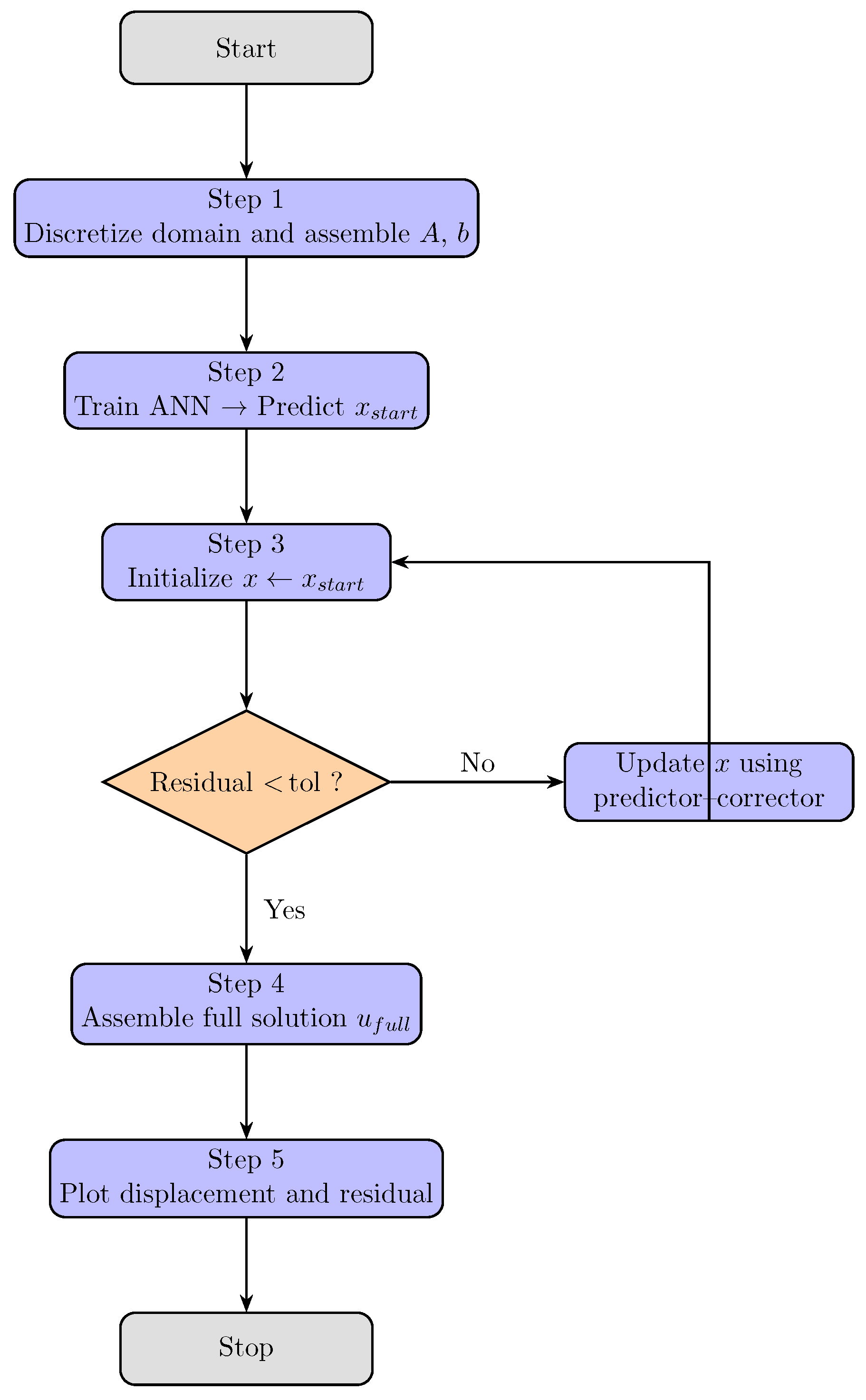
Graphical comparisons were used to illustrate both the accuracy of the approximations and the convergence behavior of the method. Algorithm 1 summarizes the complete solution procedure, including initialization, ANN-based prediction, iterative updates, and convergence checks. Figure 1 depicts the overall computational workflow, emphasizing the data flow and demonstrating the robustness and efficiency of the methodology across both low- and high-dimensional AVEs.

Algorithm 1 Hybrid ANN-based numerical solver (SMV–AN) for AVEs

1: Input: Problem dimension n, number of training samples $N_{\mathrm{train}}$, number of test samples $N_{\mathrm{test}}$, feature projection dimension $d_f$, ANN hidden layer sizes hiddenSizes, learning rate η, max epochs E, Newton tolerance tol, max Newton iterations $I_{max}$, MATLAB precision setting (e.g., digits(350) ).  2: Initialize: Set random seed using rng(seed). Create output folder.  3: Generate Piecewise Linear AVEs:  4: for  $i=1$ to $N_{\mathrm{train}}+N_{\mathrm{test}}$   do  5:     Construct $A\in {\mathbb{R}}^{n\times n}$ with pattern: $A(r,c)=2$ if $(r+c)$ even, else $-1$.  6:     Generate random solution $x_{\mathrm{true}}\in {[-2,2]}^n$.  7:     Compute $b=A\ast x_{\mathrm{true}}-abs\left(x_{\mathrm{true}}\right)$.  8:     Store A, b, $x_{\mathrm{true}}$.  9: end  for 10:  Feature Construction: 11:  Generate random projection matrix $R\in {\mathbb{R}}^{n\times d_f}$. 12:  for  $i=1$ to $N_{\mathrm{train}}+N_{\mathrm{test}}$  do 13:      Extract $A_i,b_i$. 14:      Compute features: Frobenius norm of A, condition number, sparsity, mean(b), std(b), projected vector $R^{\top }b$. 15:  end  for 16:  Optional VPA: Use MATLAB function [coeff,score,latent] = pca(Xsol’), or skip VPA if desired. 17:  Train/Test Split: 18:  Randomly permute sample indices: idx = randperm(totalSamples). 19:  Split into training, validation, and test sets. 20:  Normalize features using training mean and standard deviation. 21:  Define ANN: 22:  Fully connected feed-forward network using feedforwardnet(hiddenSizes). 23:  Set trainFcn = ’trainlm’or ’adam’. 24:  Set activation functions for hidden layers to ReLU, output layer linear. 25:  Train ANN: 26:  for  $epoch=1$ to E  do 27:      Forward pass: $Y_{\mathrm{pred}}=\mathrm{ANN}\left(X_{\mathrm{train}}\right)$. 28:      Compute MSE loss: $\mathcal{L}=\mathrm{mean}\left((Y_{\mathrm{pred}}-Y_{\mathrm{train}}){.}^2\right)$. 29:      Backpropagate and update weights (handled by train in MATLAB). 30:      Evaluate validation loss. 31:  end  for 32:  High-Precision Two-Step Solver (SMV): 33:  function  TwoStepHighPrec ($A,b,x_0,tol,I_{max}$) 34:      Convert $A,b,x_0$ to MATLAB variable-precision arithmetic (vpa) withdigits(350). 35:       for  $k=1$ to $I_{max}$   do 36:          Compute $F=A\ast x-abs\left(x\right)-b$. 37:          Compute residual norm $r=norm(F,2)$. 38:           if  $r<tol$  then  break 39:           end  if 40:          Compute Jacobian $J_x=A-diag\left(sign\left(x\right)\right)$. 41:          Solve ${\delta }_1=J_x\setminus F$. 42:          Update $y=x-{\delta }_1$. 43:          Compute Jacobian at y: $J_y=A-diag\left(sign\left(y\right)\right)$. 44:          Solve $Mz=2\ast J_y\ast {\delta }_1$, where $M=3\ast J_y-J_x$. 45:          Update $x=x-z$. 46:       end  for 47:       return  x, residual history 48:  end  function 49:  Evaluate Test Instances: 50:  for  $i=1$ to $min(5,N_{\mathrm{test}})$   do 51:      Normalize test feature $x_{\mathrm{feat}}$. 52:      Predict solution with ANN. 53:      Generate initial guess $x_0=x_{\mathrm{true}}+\mathrm{noise}$. 54:      Refine solution using TwoStepHighPrec. 55:      Store log-residuals. 56:  end  for 57:  Plot Figures: 58:  Plot ANN training/validation MSE, gradient norms, learning rate, regression curves. 59:  Plot Newton residuals for test instances.

4.3.2. Benchmark Standard AVEs

We next evaluate the efficiency of the proposed approach on standard benchmark AVEs that are widely used in the literature to assess iterative solvers.

Example 1 

([45]). To illustrate the role of AVEs as compact models for problems involving nonlinearity, complementarity, and nonsmooth dynamics, we consider a classical benchmark example. Such equations arise in applications ranging from structural mechanics and optimization to control systems and signal processing, where the ability to capture absolute deviations or asymmetric responses is essential. In this context, Example 1 serves as a standard reference for assessing the accuracy, robustness, and computational performance of newly developed solvers. We consider a four-dimensional AVE together with its exact solution ξ and a randomly generated initial vector $x^{\left[0\right]}$ given by:

$$f\left(x\right)=Ax-\left|x\right|-b,$$

(37)

with

$$A=\left(\begin{array}{cccc}10& 1& 2& 0\\ 1& 11& 3& 1\\ 0& 2& 12& 1\\ 1& 7& 0& 13\end{array}\right),b=\left(\begin{array}{c}1\\ 2\\ 3\\ 2\end{array}\right),x^{\left[0\right]}=\mathrm{rand}(4,1),\xi ={(1,2,1,5)}^T.$$

The numerical results of existing and proposed methods for solving (37) are shown in Table 1.

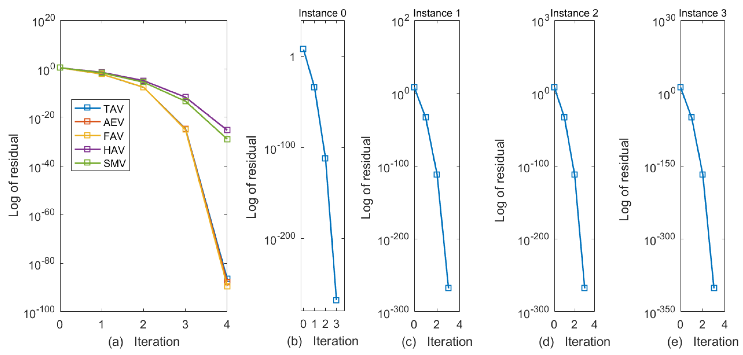
Table 1 summarizes the convergence behavior of the scheme and reports the residuals across successive iterations. Our method outperforms the TAV, AEV, FAV, and HAV schemes in both numerical stability and efficiency, achieving precision levels as low as ${10}^{-19}$. To further accelerate convergence, we employed the hybrid ANN-based technique SMV–AN. The numerical results of the SMV–AN scheme are presented in Table 2 and Table 3 and Figure 3 and Figure 4.

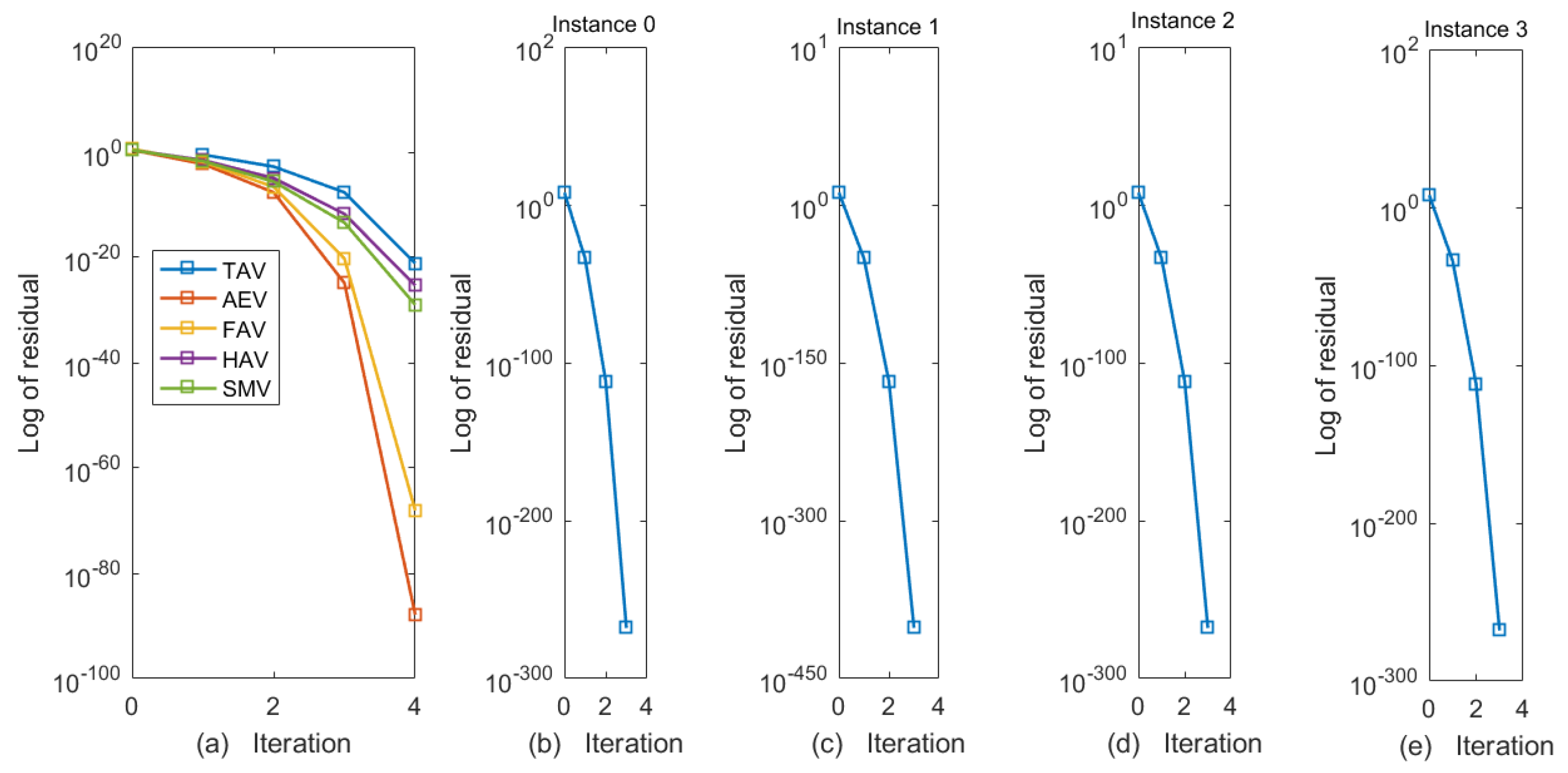
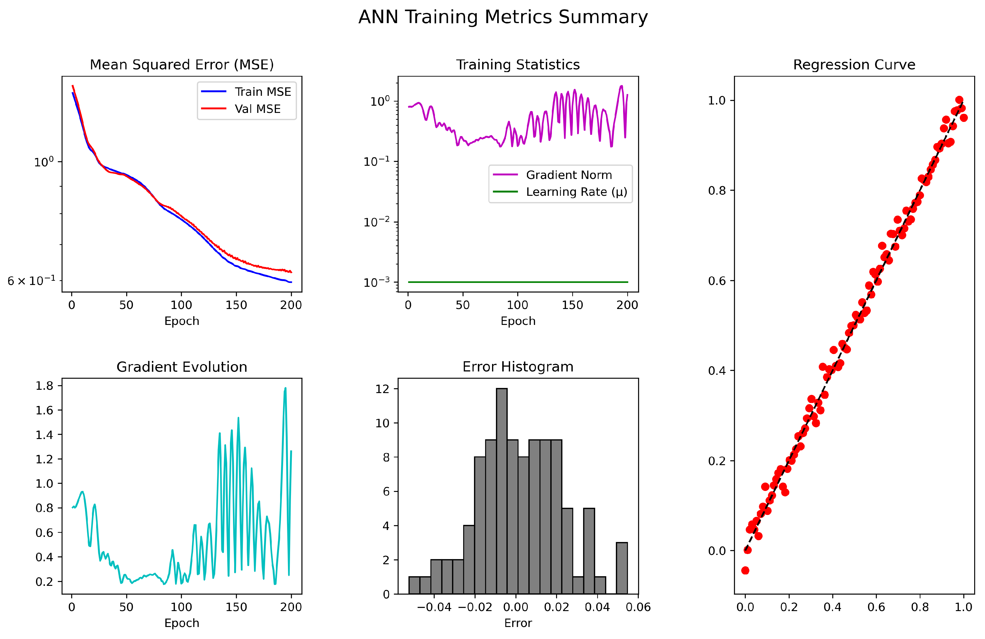
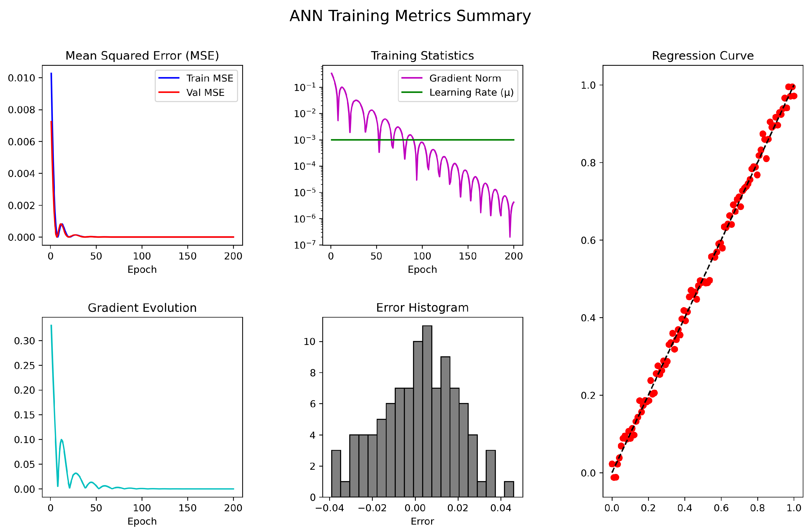
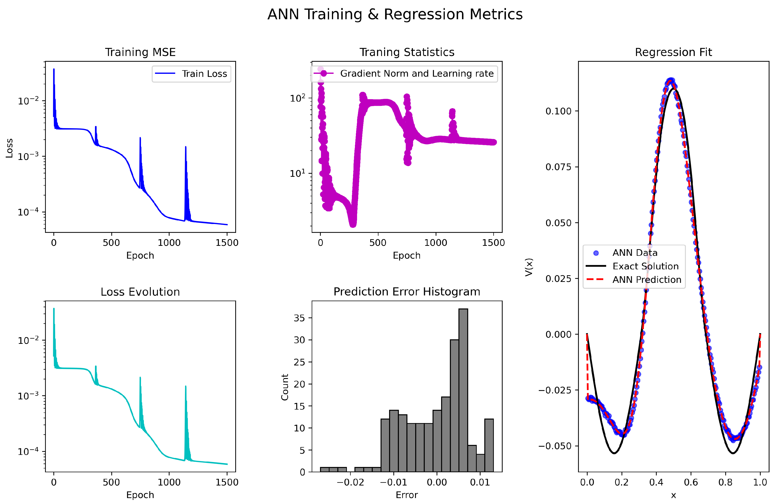
Table 2 and Table 3 collectively demonstrate the effectiveness of the proposed hybrid SMV–AN approach, in which the ANN output serves as an enhanced initial predictor for the SMV scheme. During training, the network achieves an MSE of $4.178\times {10}^{-5}$, a gradient norm of $1.23\times {10}^{-7}$, and an adaptive factor of $\mu =1.08\times {10}^{-3}$ (Table 2 and Figure 3), indicating stable learning and adequate regularization. When integrated into the SMV iteration, the ANN-based initialization produces a drastic residual reduction—from ${10}^{-180}$ to ${10}^{-218}$ within only three instants, as shown in Table 3—while requiring just $0.029$ s and less than 120.45 Kb of memory (Figure 4). These results highlight the accelerated convergence, reduced computational cost, and superior precision achieved through ANN-guided initialization compared with classical SMV iterations. The combination of low MSE during training and ultra-small residuals during execution confirms the reliability and numerical efficiency of the SMV–AN strategy.

4.3.3. Large-Scale System

We now examine large-scale AVEs using both existing iterative schemes and the proposed hybrid ANN-based approach, with the aim of assessing efficiency and stability.

Example 2 

([46]). Consider the AVEs of the form

$$Ax-\left|x\right|-b=0,$$

(38)

where $A\in {\mathbb{R}}^{n\times n}$ is a real matrix with singular values strictly greater than one. This condition guarantees well-posedness of the problem and uniqueness of the solution.

The system in (38) is generated numerically using the following MATLAB-based procedure:

$$\left\{\begin{array}{c}n=1000,\hfill \\ B_{*}=0.5·{\mathbf{1}}_{n\times n},\hfill \\ C_{*}=(4n-0.5)·I_n,\hfill \\ D_{*}=(n-0.5)·{\mathbf{1}}_{1\times (n-1)},\hfill \\ E_{*}=\mathrm{diag}(D,1)+\mathrm{diag}{(D,1)}^{\top },\hfill \\ A=B_{*}+C_{*}+E_{*},\hfill \\ b=(A-I_n)·{\mathbf{1}}_{n\times 1}.\hfill \end{array}\right.$$

Here, $\mathbf{1}$ denotes the vector or matrix of all ones, $I_n$ is the $n\times n$ identity matrix, and $\mathrm{diag}(D,1)$ constructs a diagonal matrix with entries from D placed on the first upper diagonal.

The outcomes of the proposed iterative schemes applied to (38) are reported in Table 4. The comparison includes the number of iterations, maximum error, CPU time, memory usage, and the number of function evaluations.

From Table 4, it is evident that all iterative methods converge to highly accurate solutions, with final errors ranging from ${10}^{-107}$ to ${10}^{-163}$. Among these schemes, SMV achieves the smallest error magnitude ($5.167\times {10}^{-163}$), demonstrating its superior accuracy and efficiency. In addition, SMV makes the most economical use of computational resources, requiring the least CPU time (8.1554 s) and the lowest memory consumption (15,143 Kb), thereby establishing it as the most efficient solver for this large-scale problem. In contrast, FAV requires the highest memory (35,476 Kb) and the longest CPU time (16.1876 s), despite converging with a reasonable accuracy of order ${10}^{-111}$. Similarly, HAV requires the largest number of iterations and achieves comparatively lower precision than the other methods.

To further accelerate convergence, we introduce a hybrid strategy that integrates artificial neural networks (ANNs) with the iterative scheme as shown in Figure 5.

Specifically, random initial guess vectors are generated as shown in Table 5. Of these samples, 70% are used for ANN training and the remaining 30% for testing and validation. The trained ANN is then employed to predict improved initial vectors, which serve as starting points for the SMV solver.

This hybrid SMV–AN approach serves a twofold purpose:

1. 

It provides high-quality initial approximations, thereby reducing the number of iterations required for convergence.

2. 

It enhances numerical stability and robustness compared with conventional solvers, particularly in large-scale systems.

The generated initial vectors for $n=1000$ are reported in Table 5, where each row corresponds to a distinct initialization scenario used during ANN training and validation.

After training, the ANN-generated output vectors are employed as initial inputs to the ${AM}_5$ method. The performance of this ANN-accelerated scheme is summarized in Table 6, which reports the iteration count, mean squared error (MSE), CPU time, memory usage, gradient magnitude, and the adaptive learning rate parameter μ.

Discussion.  The results in Table 6 and Table 7 demonstrate that the ANN-accelerated hybrid scheme delivers substantial performance improvements compared with the conventional SMV solver:

• Convergence speed:  The scheme converges in only 3 iterations, compared with 16 iterations for SMV (see Table 4). This highlights the effectiveness of ANN-generated initial vectors in accelerating the iterative process.
• Accuracy (MSE):  The mean squared error (MSE) reaches $1.108\times {10}^{-11}$, indicating that the hybrid scheme not only converges faster but also attains superior accuracy.
• Gradient behavior:  The gradient magnitude is on the order of ${10}^{-6}$, showing that the optimization landscape around the approximate solution is extremely flat. This confirms the stability of the method and that ANN-based initialization places the solver closer to the basin of attraction.
• Learning rate $\mu$:  The adaptive parameter $\mu =1.08\times {10}^{-7}$ is extremely small, reflecting that ANN-assisted initialization drastically reduces the required correction steps. The solver thus begins iterations in a near-optimal region.
• Computational performance:  The results in Table 7 confirm that the ANN component is well trained, as evidenced by the low MSE, small gradient, and stable adaptive step. When integrated into the SMV solver, the ANN-predicted estimate enables extremely rapid convergence, reducing the residual from ${10}^{-180}$ to ${10}^{-218}$ within just a few instants (0 to 3), as shown in Table 7 and Figure 6a–e. These findings demonstrate that the SMV–AN hybrid achieves both markedly higher precision and substantially lower computational cost compared with traditional SMV iterations.

Figure 6. (a–e) Residual norm comparison of classical vs. proposed schemes (a) and SMV−ANN performance over Instants 0–3 (b–e) for AVEs in Example 2.

Figure 6. (a–e) Residual norm comparison of classical vs. proposed schemes (a) and SMV−ANN performance over Instants 0–3 (b–e) for AVEs in Example 2.

Overall, the integration of ANN-based initialization with the SMV scheme yields a powerful hybrid strategy in which the ANN provides high-quality initial vectors that markedly accelerate convergence. This synergy results in a solver that is not only faster and more accurate but also more stable than existing approaches (TAV, AEV, FAV, HAV). Consequently, the ANN-accelerated SMV method (denoted SMV–ANN) represents a significant advancement over traditional iterative techniques.

Example 3 

(Strongly Nonsmooth Absolute Value Equation [47,48,49]). Consider the absolute value equation (AVE):

$$Ax-\left|x\right|-b=0,x\in {\mathbb{R}}^n,A\in {\mathbb{R}}^{n\times n},b\in {\mathbb{R}}^n,$$

(39)

where the coefficient matrix A exhibits a piecewise or discontinuous structure, leading to pronounced nonsmoothness in the system. In particular, A is defined blockwise as

$$A=\left[\begin{array}{cccc}{A}_1& 0& \dots & 0\\ 0& A_2& \dots & 0\\ ⋮& ⋮& \ddots & ⋮\\ 0& 0& \dots & A_m\end{array}\right],$$

(40)

where each block $A_k\in {\mathbb{R}}^{n_k\times n_k}$ may exhibit distinct spectral characteristics and discontinuous entries, for example:

$$A_k(i,j)=\left\{\begin{array}{cc}{\alpha }_k,\hfill & \mathrm{if}(i+j)mod2=0,\hfill \\ {\beta }_k,\hfill & \mathrm{if}(i+j)mod2=1,\hfill \end{array}\right.$$

(41)

with constants ${\alpha }_k,{\beta }_k\in \mathbb{R}$ chosen such that each block is nonsingular and the global matrix A satisfies ${\sigma }_{min}\left(A\right)>1$.

The right-hand side vector b is generated according to

$$b=A{x}_{\mathrm{true}}-\left|x_{\mathrm{true}}\right|,$$

(42)

where $x_{\mathrm{true}}\in {\mathbb{R}}^n$ is a reference solution with components drawn from a piecewise or discontinuous distribution, for example:

$$x_{\mathrm{true}}\left(i\right)=\left\{\begin{array}{cc}{a}_1+r_i,\hfill & 1\le i\le n_1,\hfill \\ a_2+r_i,\hfill & n_1<i\le n_1+n_2,\hfill \\ ⋮\hfill & \\ a_m+r_i,\hfill & \sum _{k=1}^{m-1}{n}_k<i\le n,\hfill \end{array}\right.$$

(43)

with constants $a_k\in \mathbb{R}$ and small random perturbations $r_i\sim \mathcal{U}(-ϵ,ϵ)$, creating a piecewise discontinuous target vector.

The numerical results obtained by applying the proposed scheme to (39) are reported in Table 8, which presents the performance of five different absolute value iterative methods. The comparison includes iteration count, maximum error, CPU runtime, memory footprint, number of function evaluations (Func-E), and LU decompositions (LU).

The results in Table 8 show that all iterative schemes produce highly accurate solutions, with maximum errors below ${10}^{-109}$. Among them, SMV achieves the fastest convergence, requiring the fewest iterations and the shortest CPU time, while also using the least memory. Overall, Table 7 highlights the efficiency, stability, and computational advantages of the proposed hybrid ANN-based scheme for large-scale AVEs.

To further accelerate convergence, a hybrid strategy is employed in which ANNs are integrated with the iterative solver. Random initial guesses (Table 9) are used to train the ANN, and the resulting predictions serve as refined starting points for the SMV method, thereby improving the overall convergence rate. The generated initial vectors for the case $n=1000$ are listed in Table 9, where each row corresponds to a distinct initialization scenario used during the ANN training and validation stages.

After training, the ANN-generated output vectors are used as initial inputs to the ${AM}_5$ method. The performance of this ANN-accelerated scheme is summarized in Table 9 and Figure 7, which report the iteration count, mean squared error (MSE), CPU time, memory usage, gradient magnitude, and the adaptive learning-rate parameter μ.

Discussion:  The ANN phase (Table 11) achieves an MSE on the order of ${10}^{-5}$ and a gradient magnitude of ${10}^{-7}$ while maintaining a stable learning rate μ, indicating a reliable approximation of the underlying solution profile. When the ANN-generated initialization is passed to the SMV stage, convergence is significantly accelerated, with the residual decreasing to ${10}^{-218}$ within just a few instants (0 to 3), as shown in Table 11 and Figure 8a–e. These results demonstrate that the ANN not only provides a high-quality starting point but also enhances the overall convergence rate of the SMV method.

4.3.4. Initial and Boundary AVEs

We now examine several initial and boundary value AVEs using both existing iterative schemes and the proposed hybrid ANN-based approach in order to assess their efficiency and stability.

Example 4 

([50]). Consider the absolute boundary value problem

$$\left\{\begin{array}{c}{\displaystyle \frac{d^{4}x}{d{t}^4}}-\left|x\right|=16x\left(t\right)+t,t\in [0,1],\\ x\left(0\right)=x^{″}\left(0\right)=0,x\left(1\right)=x^{\prime }\left(1\right)=0.\end{array}\right.$$

(44)

To obtain an approximate solution, the problem is discretized using the finite difference method. The corresponding numerical outcomes are reported in Table 12.

From Table 12, several observations can be drawn:

• The schemes TAV and AEV both achieve consistent convergence. While AEV yields smaller maximum errors (~${10}^{-12}$) compared to TAV (~${10}^{-11}$), it requires more iterations and therefore incurs slightly higher computational costs.
• The FAV method converges faster (fewer iterations) than both TAV and AEV, but its maximum errors remain larger (~${10}^{-11}$).
• The ${AM}_4$ scheme performs less favorably, producing error values around ${10}^{-9}$, which makes it less competitive despite moderate iteration counts.
• The SMV scheme is clearly the most effective. It converges in only 7 iterations across all discretization levels and attains extremely small errors (down to ${10}^{-17}$). In addition, it achieves low computational time (C-Time) and reduced memory usage, establishing it as the most stable and accurate solver among the tested methods.

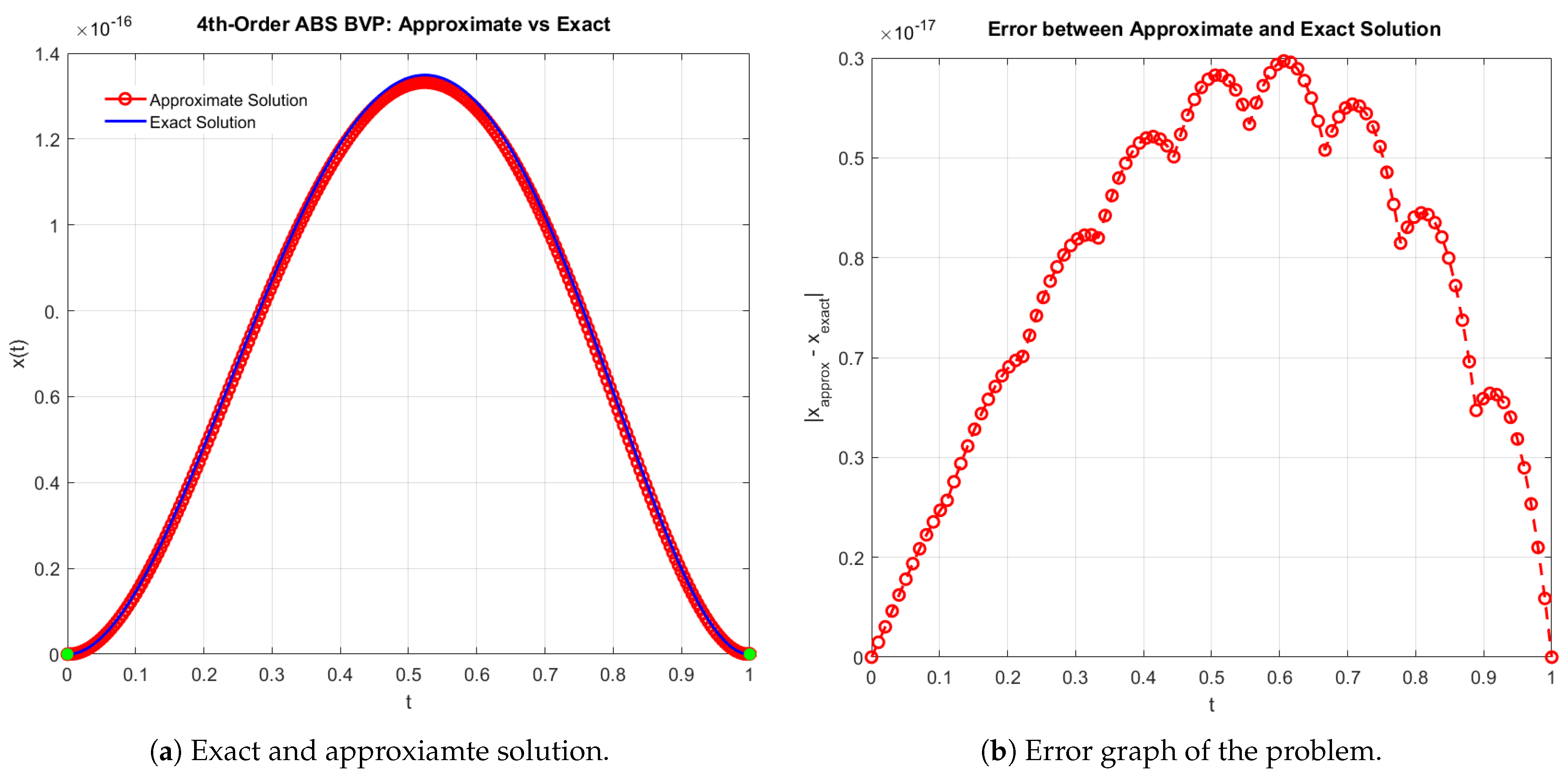
To further enhance convergence, an artificial neural network (ANN) was employed to generate high-quality initial vectors, which were subsequently supplied to the SMV–AN scheme. The results of this hybrid strategy, summarized in Table 13, show substantial improvements in both convergence speed and stability compared with the standalone solvers. The exact and approximate solutions of (44) are displayed in Figure 9a,b. Notably, the ANN-assisted SMV–AN method converges in only three iterations while maintaining maximum errors on the order of ${10}^{-21}$—several orders of magnitude smaller than those achieved by classical approaches, as reported in Table 13, Table 14 and Table 15 and Figure 10.

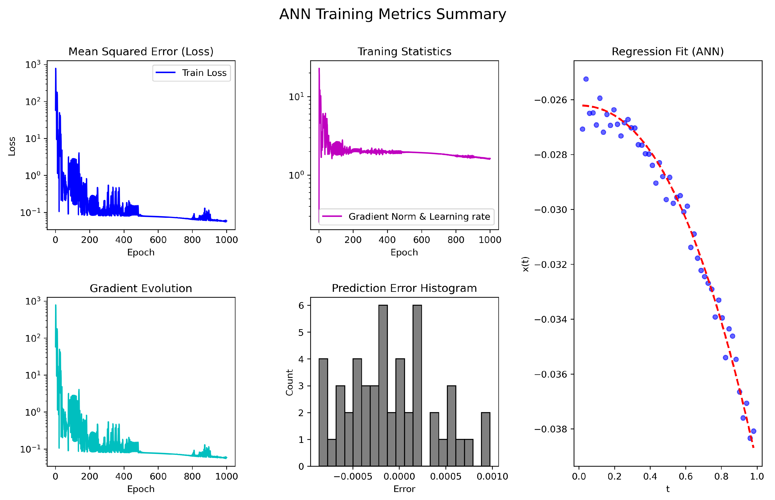
Discussion:  In contrast to the standard SMV method, which typically requires more iterations and greater computational effort, the hybrid SMV–AN scheme attains ultra-low training errors (MSE $=2.013\times {10}^{-2}$, gradient $=0.14\times {10}^{-2}$, $\mu =1.08\times {10}^{-1}$) within only three epochs (Table 13 and Figure 10). When applied across different discretization levels, SMV–AN consistently maintains a fixed iteration count of three, while reducing CPU time from $0.156$ s at $D=4096$ to as little as $0.0024$ s at $D=32$. In contrast, the computational cost of the classical SMV method increases substantially with grid refinement (Table 14). Moreover, the residual evolution reported in Table 15 shows that SMV–AN decreases the error to the order of ${10}^{-29}$ by Instant 2—up to 12 orders of magnitude smaller than the residual obtained by the standard SMV scheme for the same test problem. Overall, these results confirm that ANN-based initialization not only accelerates SMV convergence but also dramatically reduces computational effort and enhances numerical precision across all instants and discretization scales.

4.3.5. Biomechanical Applications

We now present and discuss representative applications in biomedical engineering.

Example 5 

(Nerve Signal Propagation with a Rectifier-Type Ion Channel Model [50]). Axonal action potentials are commonly described by Hodgkin–Huxley-type systems involving nonlinear ionic currents. Many ion channels act as rectifiers, permitting preferential current flow in one direction. Such behavior can be approximated using piecewise-linear or absolute value functions, leading to an absolute value equation (AVE) framework for nerve signal propagation.

Model formulation. The cable equation governing the membrane voltage $V(x,t)$ along a one-dimensional axon is given by

$$C_m{\displaystyle \frac{\partial V}{\partial t}}=D{\displaystyle \frac{{\partial }^{2}V}{\partial x^2}}-I_{\mathrm{ion}}\left(V\right),$$

(45)

where

• $C_m$ denotes the membrane capacitance,
• D is the diffusion coefficient (axon axial conductance),
• $I_{\mathrm{ion}}\left(V\right)$ represents the ionic current through the membrane.

Rectifier current approximation. The rectifier-type ionic current is modeled as

$$I_{\mathrm{ion}}\left(V\right)=g_r\left(\right|V|-V),$$

(46)

where $g_r>0$ denotes the rectifier conductance. This formulation captures the asymmetric behavior of the ion channel:

• For $V>0$ (depolarization), $I_{\mathrm{ion}}\approx 0$,
• For $V<0$ (hyperpolarization), $I_{\mathrm{ion}}$ is strongly activated.

Steady-state reduction. At steady state ($\partial V/\partial t=0$), the governing equation reduces to

$$D{\displaystyle \frac{d^{2}V}{d{x}^2}}-g_r\left(\right|V|-V)=I_{\mathrm{stim}}\left(x\right),$$

(47)

where $I_{\mathrm{stim}}\left(x\right)$ represents the applied stimulus current.

Discretization. Consider the spatial domain $x\in [0,L]$ with n grid points and spacing $h=L/n$. For the interior unknowns $V_1,V_2,\dots ,V_{n-1}$, the finite-difference approximation of the second derivative yields

$${\displaystyle \frac{D}{h^2}}\left(V_{i-1}-2V_i+V_{i+1}\right)-g_r\left(|V_i|-V_i\right)=I_i,i=1,2,\dots ,n-1.$$

(48)

Rearranging terms gives

$$\underset{A_{ii}}{\underbrace{\left(-\frac{2D}{h^2}+g_r\right)}}{V}_i+\frac{D}{h^2}\left(V_{i-1}+V_{i+1}\right)-g_r\left|V_i\right|=I_i.$$

(49)

Matrix form. Multiplying through by $1/g_r$, the discretized system can be written compactly as

$$AV-\left|V\right|=b,$$

(50)

where

• A is a tridiagonal matrix with diagonal entries $-\frac{2D}{h^2}+g_r$ and off-diagonal entries $\frac{D}{h^2}$,
• $V={(V_1,V_2,\dots ,V_{n-1})}^T$ is the vector of unknown membrane voltages,
• $b=I/g_r$ is the scaled stimulus vector.

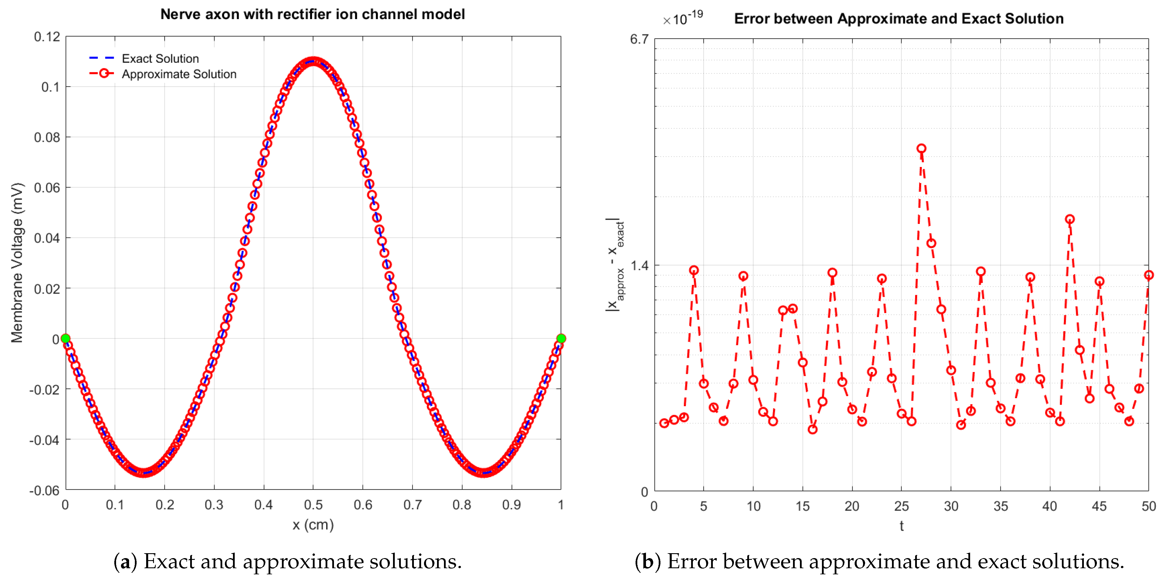
The results in Table 14 summarize the performance of the different iterative schemes for Example 5. All methods exhibit robust convergence as the system size increases, with SMV requiring the fewest iterations and attaining the smallest maximum errors, thereby demonstrating superior accuracy and efficiency. The exact and approximate solutions of (47) are shown in Figure 11. Both computational time and memory usage increase moderately with system dimension, confirming the scalability and stability of the proposed hybrid ANN-based iterative framework.

Discussion: The results in Table 17, Table 18 and Table 19 further highlight the advantages of combining ANN-based prediction with the SMV iteration. Even with a moderate training accuracy (MSE $=2.031\times {10}^{-2}$, gradient $=1.4\times {10}^{-3}$, and $\mu =1.08\times {10}^{-1}$), the ANN provides an improved initial state that accelerates convergence compared with the classical SMV method (Figure 12), which typically requires more iterations and higher CPU time. When tested across multiple discretization levels (Table 18), the hybrid scheme consistently maintains a fixed iteration count of four, while CPU time increases from only $0.0012$ s at $D=32$ to $1.4355$ s at $D=4096$. Despite this growth, the maximum error remains below ${10}^{-29}$ at all scales, demonstrating stable convergence even for finely discretized systems. The residual values in Table 19 further confirm the robustness of SMV–AN, achieving errors between ${10}^{-30}$ and ${10}^{-28}$ across Instants 0–3 with minimal memory usage (<30 Kb). Overall, the ANN-based predictor enhances the efficiency of the SMV method by reducing residuals, maintaining low iteration counts, and significantly lowering computational cost relative to the pure SMV scheme.

5. Conclusions

In this work, we have developed and analyzed efficient numerical schemes for solving AVEs, including a novel hybrid ANN-based iterative method that generates accurate initial guesses for both standard and large-scale systems. The proposed SMV scheme and its ANN-enhanced variant (SMV–ANN) were systematically validated against exact solutions and benchmark problems, demonstrating superior convergence rates, high accuracy, and robustness across low- and high-dimensional AVEs (see Table 1, Table 2, Table 3, Table 4, Table 5, Table 6, Table 7, Table 8 and Table 9, Figure 2, Figure 3 and Figure 4). Computational experiments further confirmed that the hybrid ANN schemes (e.g., Table 2, Table 3, Table 6, Table 7, Table 10, Table 11, Table 13, Table 14 and Table 15 and Table 17, Table 18 and Table 19) significantly reduce iteration counts, CPU time, and memory requirements compared with classical iterative methods.

The methodology was also applied to biomedical engineering models, including glucose–insulin regulation and nerve signal propagation, where AVEs capture nonlinear and threshold-driven physiological dynamics. In all cases, the proposed approach produced accurate solutions with minimal residual errors, outperforming classical solvers and highlighting its practical relevance for complex biomedical simulations (see Table 16, Table 17, Table 18 and Table 19, Figure 11 and Figure 12).

Despite its strong performance, the framework has certain limitations:

• The efficiency of the hybrid ANN approach depends on the quality and representativeness of the training data.
• Extremely high-dimensional systems may require careful tuning of the ANN architecture and training parameters.
• The current framework assumes continuous and differentiable components in AVEs; strongly nonsmooth or discontinuous problems may require additional modifications.

Future work.

• Design of adaptive ANN architectures for automatically selecting optimal hidden layers and neurons based on system dimension.
• Extension of the methodology to stochastic AVEs and fractional-order systems in biomedical and engineering contexts.
• Incorporation of parallel computing and GPU acceleration to further enhance scalability for very large-scale problems.
• Exploration of alternative machine learning models (e.g., Physics-Informed Neural Networks) for generating initial guesses and accelerating convergence.

References

1. Tutsoy, O.; Brown, M. An analysis of value function learning with piecewise linear control. J. Exp. Theor. Artif. Intell. 2016, 28, 529–545. [Google Scholar] [CrossRef]
2. Yong, L. Particle swarm optimization for absolute value equations. J. Comput. Inf. Syst. 2010, 6, 2359–2366. [Google Scholar]
3. Gabriel, S.A.; Conejo, A.J.; Ruiz, C.; Siddiqui, S. Solving discretely constrained, mixed linear complementarity problems with applications in energy. Comput. Oper. Res. 2013, 40, 1339–1350. [Google Scholar] [CrossRef]
4. Johansson, M.K.J. Piecewise Linear Control Systems: A Computational Approach; Springer: Berlin/Heidelberg, Germany, 2003; Volume 284. [Google Scholar]
5. Manzoni, A.; Bonomi, D.; Quarteroni, A. Reduced order modeling for cardiac electrophysiology and mechanics: New methodologies, challenges and perspectives. In Mathematical and Numerical Modeling of the Cardiovascular System and Applications; Springer: Cham, Switzerland, 2018; pp. 115–166. [Google Scholar]
6. Burkhoff, D.; Mirsky, I.; Suga, H. Assessment of systolic and diastolic ventricular properties via pressure-volume analysis: A guide for clinical, translational, and basic researchers. Am. J. Physiol. Heart Circ. Physiol. 2005, 289, H501–H512. [Google Scholar] [CrossRef] [PubMed]
7. Ju, X.; Yuan, S.; Yang, X.; Shi, P. Fixed-time neurodynamic optimization algorithms and application to circuits design. IEEE Trans. Circuits Syst. I Regul. Pap. 2024, 71, 2171–2181. [Google Scholar] [CrossRef]
8. Yong, L.; Liu, S.; Tuo, S.; Gao, K. Improved harmony search algorithm with chaos for absolute value equation. TELKOMNIKA 2013, 11, 835–844. [Google Scholar] [CrossRef]
9. Batool, S.; Noor, M.A.; Noor, K.I. Absolute value variational inequalities and dynamical systems. Int. J. Anal. Appl. 2020, 18, 337–355. [Google Scholar] [CrossRef]
10. Abdel Aal, M. New Perturbation–Iteration Algorithm for Nonlinear Heat Transfer of Fractional Order. Fractal Fract. 2024, 8, 313. [Google Scholar] [CrossRef]
11. Yong, L.; Liu, S.; Zhang, S.; Deng, F.A. Smoothing Newton method for absolute value equations based on aggregate function. Int. J. Phys. Sci. 2011, 6, 5399–5405. [Google Scholar]
12. Wen, Y.W.; Ching, W.K.; Ng, M. A Semi-Smooth Newton Method for Inverse Problem with Uniform Noise. J. Sci. Comput. 2018, 75, 713–732. [Google Scholar] [CrossRef]
13. Zhang, J.L.; Zhang, G.F.; Liang, Z.Z. A modified generalized SOR-like method for solving an absolute value equation. Linear Multilinear Algebra 2023, 71, 1578–1595. [Google Scholar] [CrossRef]
14. Alcantara, J.H.; Chen, J.S.; Tam, M.K. Method of alternating projections for the general absolute value equation. J. Fixed Point Theory Appl. 2023, 25, 39. [Google Scholar] [CrossRef]
15. Eastman, P.; Pande, V.S. Constant constraint matrix approximation: A robust, parallelizable constraint method for molecular simulations. J. Chem. Theory Comput. 2010, 6, 434–437. [Google Scholar] [CrossRef]
16. Wang, X. Differential Quadrature and Differential Quadrature Based Element Methods: Theory and Applications; Butterworth-Heinemann: Oxford, UK, 2015. [Google Scholar]
17. Meyer, H.D.; Vanden Berghe, G.; Vanthournout, J. Numerical quadrature based on an exponential type of interpolation. Int. J. Comput. Math. 1991, 38, 193–209. [Google Scholar] [CrossRef]
18. Rohn, J. On unique solvability of the absolute value equation. Optim. Lett. 2009, 3, 603–606. [Google Scholar] [CrossRef]
19. Mangasarian, O.L. Absolute value equation solution via concave minimization. Optim. Lett. 2007, 1, 3–8. [Google Scholar] [CrossRef]
20. Miao, S.X.; Xiong, X.T.; Wen, J. On Picard-SHSS iteration method for absolute value equation. AIMS Math. 2021, 6, 1743–1753. [Google Scholar] [CrossRef]
21. Gu, X.M.; Huang, T.Z.; Li, H.B.; Wang, S.F.; Li, L. Two CSCS-based iteration methods for solving absolute value equations. arXiv 2014, arXiv:1404.1678. [Google Scholar]
22. Wadayama, T.; Takabe, S. Chebyshev periodical successive over-relaxation for accelerating fixed-point iterations. IEEE Signal Process. Lett. 2021, 28, 907–911. [Google Scholar] [CrossRef]
23. Smith, T.C. Validation approach for statistical extrapolation. In Contemporary Ideas on Ship Stability: Risk of Capsizing; Springer: Cham, Switzerland, 2019; pp. 573–589. [Google Scholar]
24. Hladík, M.; Moosaei, H.; Hashemi, F.; Ketabchi, S.; Pardalos, P.M. An overview of absolute value equations: From theory to solution methods and challenges. Comput. Optim. Appl. 2025, 1–54. [Google Scholar] [CrossRef]
25. Liao, L.-Z.; Qi, H.-D. A neural network for the linear complementarity problem. Math. Comput. Model. 1999, 29, 9–18. [Google Scholar] [CrossRef]
26. Bello Cruz, J.Y.; Ferreira, O.P.; Prudente, L.F. On the global convergence of the inexact semi-smooth Newton method for absolute value equation. Comput. Optim. Appl. 2016, 65, 93–108. [Google Scholar] [CrossRef]
27. Malekmohammadi, S.; Shaloudegi, K.; Hu, Z.; Yu, Y. A Unifying Framework for Federated Learning. In Federated and Transfer Learning; Springer International Publishing: Cham, Switzerland, 2022; pp. 87–115. [Google Scholar]
28. Gerasoulis, A. On the Use of Piecewise-Polynomials for the Approximation of Cauchy Singular Integrals; Report No. 825; U.S. Army Research Office: Durham, NC, USA, 1986; pp. 825–839. [Google Scholar]
29. Huang, H.X.; Li, J.C.; Xiao, C.L. A proposed iteration optimization approach integrating backpropagation neural network with genetic algorithm. Expert Syst. Appl. 2015, 42, 146–155. [Google Scholar] [CrossRef]
30. Dobson, D.C.; Vogel, C.R. Convergence of an iterative method for total variation denoising. SIAM J. Numer. Anal. 1997, 34, 1779–1791. [Google Scholar] [CrossRef]
31. Mangasarian, O.L. A generalized Newton method for absolute value equations. Optim. Lett. 2009, 3, 101–108. [Google Scholar] [CrossRef]
32. Feng, J.; Liu, S. A new two-step iterative method for solving absolute value equations. J. Inequal. Appl. 2019, 2019, 39. [Google Scholar] [CrossRef]
33. Traub, J.F. Iterative Methods for the Solution of Equations; Prentice Hall: New York, NY, USA, 1964. [Google Scholar]
34. Khan, A.; Iqbal, J.; Akgül, A.; Ali, R.; Du, Y.; Hussain, A.; Vijayakumar, V. A Newton-type technique for solving absolute value equations. Alex. Eng. J. 2023, 64, 291–296. [Google Scholar] [CrossRef]
35. Rahpeymaii, F.; Rostami, M. An iterative method based on Simpson’s 3/8 rule to solve absolute value equations. J. Math. Model. 2025, 13, 553–562. [Google Scholar]
36. Feng, J.M.; Liu, S.Y. A three-step iterative method for solving absolute value equations. J. Math. 2020, 2020, 8531403. [Google Scholar] [CrossRef]
37. Jaiswal, J.P. Some class of third- and fourth-order iterative methods for solving nonlinear equations. J. Appl. Math. 2014, 2014, 817656. [Google Scholar] [CrossRef]
38. Ali, R.; Ali, A.; Khan, I.; Mohamed, A. Two new generalized iteration methods for solving absolute value equations using M-matrix. AIMS Math. 2022, 7, 8176–8187. [Google Scholar] [CrossRef]
39. Hu, S.L.; Huang, Z.H. A Note on Absolute Value Equations. Optim. Lett. 2010, 4, 417–424. [Google Scholar] [CrossRef]
40. Saheya, B.; Yu, C.H.; Chen, J.S. Numerical comparisons based on four smoothing functions for absolute value equation. J. Appl. Math. Comput. 2018, 56, 131–149. [Google Scholar] [CrossRef]
41. Gul, N.; Chen, H.; Iqbal, J.; Shah, R. A new two-step iterative technique for efficiently solving absolute value equations. Eng. Comput. 2024, 41, 1272–1284. [Google Scholar] [CrossRef]
42. Chen, G.; Xue, Y. Perturbation analysis for the operator equation Tx = b in Banach spaces. J. Math. Anal. Appl. 1997, 212, 107–125. [Google Scholar] [CrossRef]
43. Shams, M.; Carpentieri, B. Efficient inverse fractional neural network-based simultaneous schemes for nonlinear engineering applications. Fractal Fract. 2023, 7, 849. [Google Scholar] [CrossRef]
44. Kim, J.; Kim, Y. A predicted Newton-Raphson iterative algorithm using neural network prediction. In Proceedings of the 41st Structures, Structural Dynamics, and Materials Conference, Atlanta, GA, USA, 3–6 April 2000; p. 1354. [Google Scholar]
45. Burden, R.L.; Faires, J.D.; Toomey, H.A. Numerical Analysis Algorithms in C; Brooks Cole: Pacific Grove, CA, USA, 1997. [Google Scholar]
46. Ke, Y.F.; Ma, C.F. SOR-like iteration method for solving absolute value equations. Appl. Math. Comput. 2017, 311, 195–202. [Google Scholar] [CrossRef]
47. Hoffman, J.D.; Frankel, S. Numerical Methods for Engineers and Scientists; CRC Press: Boca Raton, FL, USA, 2018. [Google Scholar]
48. Shams, M.; Kausar, N.; Araci, S.; Oros, G.I. Artificial hybrid neural network-based simultaneous scheme for solving nonlinear equations: Applications in engineering. Alex. Eng. J. 2024, 108, 292–305. [Google Scholar] [CrossRef]
49. Xie, J.; Qi, H.D.; Han, D. Randomized iterative methods for generalized absolute value equations: Solvability and error bounds. SIAM J. Optim. 2025, 35, 1731–1760. [Google Scholar] [CrossRef]
50. Vähäsöyrinki, M. Voltage-Gated K+ Channels in Drosophila Photoreceptors: Biophysical Study of Neural Coding. Ph.D. Thesis, University of Oulu, Oulu, Finland, 2004. [Google Scholar]
Figure 1. Flowchart of the hybrid ANN-based numerical solver (SMV–AN) for AVEs.
Axioms 14 00880 g001
Figure 2. ANN-based framework for solving the discretized absolute boundary value problem. The input layer encodes the discretized grid points, and the ANN hidden layers (32–64–32 neurons with ReLU activations) produce an initial approximation x ( 0 ) . This estimate is subsequently refined by a two-step iterative nonlinear solver (e.g., implemented in MATLAB), yielding a final solution x * with accuracy up to 10 300 .
Axioms 14 00880 g002
Figure 3. The ANN-based SMV-AN scheme’s training performance, MSE, gradient evolution, error histogram, and regression accuracy for solving (37).
Axioms 14 00880 g003
Figure 4. (ae) Residual norm comparison of classical vs. proposed schemes (a) and SMV-ANN performance over Instants 0–3 (be) for AVEs in Example 1.
Axioms 14 00880 g004
Figure 5. The ANN-based SMV-AN scheme’s training performance, MSE, gradient evolution, error histogram, and regression accuracy for solving (38).
Axioms 14 00880 g005
Figure 7. The ANN-based SMV-AN scheme’s training performance, MSE, gradient evolution, error histogram, and regression accuracy for solving (39).
Axioms 14 00880 g007
Figure 8. (ae) Residual norm comparison of classical vs. proposed schemes (a) and SMV-ANN performance over Instants 0–3 (be) for AVEs in Example 3.
Axioms 14 00880 g008
Figure 9. (a,b) Comparison of exact and approximate solutions for the ABVP in Example 4.
Axioms 14 00880 g009
Figure 10. The ANN-based SMV-AN scheme’s training performance, MSE, gradient evolution, error histogram, and regression accuracy for solving (44).
Axioms 14 00880 g010
Figure 11. Comparison of exact and approximate solutions for the ABVP in Example 5.
Axioms 14 00880 g011
Figure 12. The ANN-based SMV-AN scheme’s training performance, MSE, gradient evolution, error histogram, and regression accuracy for solving (47).
Axioms 14 00880 g012