Abstract
The transportation problem (TP) is a canonical linear programming model for minimizing the cost of distributing goods from multiple sources to multiple destinations. Classical TPs assume deterministic costs, supplies, and demands, whereas real supply chains are affected by volatility in fuel prices, inflation, disruptions, and weather, making such parameters uncertain. Fuzzy sets (FSs) and intuitionistic fuzzy sets (IFSs) have been widely used to handle vagueness; however, while Atanassov’s IFSs incorporate hesitation in addition to membership and non-membership, they remain limited to isotropic representations of uncertainty. This paper introduces an index-matrix interpretation for a two-stage three-dimensional transportation problem (2-S 3-D TP) defined under Elliptic Intuitionistic Fuzzy Quadruples (E-IFQs). Within this framework, transportation costs, supplies, and demands are represented as E-IFQs, allowing the modeling of anisotropic and correlated uncertainty along the membership and non-membership axes. The two-stage formulation extends previous intuitionistic fuzzy approaches by adding a temporal dimension and incorporating practical constraints such as cost thresholds and feasibility checks. The objective is to determine optimal producer–hub–buyer allocations that minimize the total E-IFQ cost while preserving consistency across all stages and time periods. A detailed case study on EV battery module distribution demonstrates the effectiveness of the proposed model. Compared with conventional fuzzy and intuitionistic fuzzy formulations, the 2-S 3-D E-IFTP yields more robust and precise decisions under complex, multidimensional uncertainty, offering improved interpretability and policy integration over time.
Keywords:
Elliptic Intuitionistic Fuzzy Quadruples (E-IFQs); EV battery distribution; index-matrix interpretation; multi-stage logistics optimization; supply chain uncertainty; transportation problem MSC:
90B06; 90C70; 90C90; 03E72
1. Introduction
Transportation problems (TPs) are classical optimization models that aim to minimize the cost of distributing goods from multiple sources to multiple destinations while satisfying supply and demand constraints. Since the pioneering works of Hitchcock [1], Dantzig [2], and Kantorovich [3], TPs have become fundamental in logistics, supply chain management, and resource allocation. In real-world logistics, however, transportation costs, supplies, and demands are rarely deterministic. Uncertainty arises from factors such as fluctuating fuel prices, inflation, road and port conditions, weather disruptions, and socio-economic instabilities. To capture such variability, fuzzy logic has proven to be a powerful modeling tool for vagueness and imprecision. Zadeh’s fuzzy sets (FSs) [4] established the foundation, while Atanassov’s intuitionistic fuzzy sets (IFSs) [5] extended it by introducing hesitation degrees in addition to membership and non-membership. Over the years, numerous fuzzy extensions have been employed in transportation problems, including trapezoidal and triangular fuzzy numbers [6,7], the intuitionistic fuzzy method of potentials [8], the Intuitionistic Fuzzy Zero Point Method (IFZPM) [9], and hybrid fuzzy transportation models with multi-objective optimization under fully intuitionistic fuzzy parameters [10]. A comprehensive overview of fuzzy transportation and trans-shipment problems is presented in [11]. More recently, Atanassov introduced Elliptic Intuitionistic Fuzzy Sets (E-IFSs) [12], which generalize IFSs by representing uncertainty in elliptical domains instead of intervals [13] or circles [14]. This enables anisotropic modeling, where imprecision in membership and non-membership degrees varies with orientation, allowing for a more realistic characterization of correlated uncertainties. Despite these advances, applications of E-IFSs to transportation problems remain scarce. Existing studies are mainly confined to franchise selection, multi-criteria decision making (MCDM, [15]), or two-dimensional distribution settings. To bridge this gap, we propose a novel two-stage, three-dimensional transportation model based on Elliptic Intuitionistic Fuzzy Quadruples (E-IFQs) and solved via an index-matrix interpretation. The model captures uncertainty in transportation costs, supply, and demand while incorporating practical constraints such as cost thresholds.
The key contributions of this paper are as follows:
- Formulation of a two-stage three-dimensional transportation problem under E-IFQs (2-S 3-D E-IFTP);
- Development of an index-matrix solution algorithm that generalizes earlier intuitionistic fuzzy methods;
- Validation of the proposed approach through a detailed case study on the distribution of EV battery modules across a multi-stage supply chain under uncertainty.
The remainder of the paper is organized as follows. Section 2 reviews related fuzzy and intuitionistic fuzzy approaches. Section 3 introduces preliminaries on E-IFQs and index matrices. Section 4 presents the proposed model and algorithm. Section 5 provides a numerical case study and analysis. Section 6 and Section 7 conclude the paper with remarks and outline directions for future research.
2. Review of Literature on Transportation Problems Under Uncertainty
Transportation problems (TPs) are one of the classical classes of linear programming models. The initial formulations of Hitchcock [1], Dantzig [2], and Kantorovich [3] laid the mathematical foundation for optimal allocation of resources. Subsequently, various extensions have been proposed to address practical issues such as multi-stage flows, higher dimensionality, and additional side constraints.
Uncertainty in transportation data has motivated the use of fuzzy set theory, introduced by Zadeh [4], which allows the modeling of imprecise costs, supplies, and demands. Several authors have developed fuzzy approaches for solving transportation problems. Chanas and Kuchta [16] and Chanas et al. [17] presented early formulations of fuzzy transportation problems. Jimenez and Verdegay [18] and Liang [19] introduced approaches based on ranking functions and fuzzy programming. Further contributions by Liu and Kao [20,21] provided methods for trapezoidal fuzzy parameters, while Pandian and Natarajan [22] proposed the Zero Point Method (ZPM). Other allocation-based methods include those of Kaur and Kumar [23], Guzel [24], and Basirzadeh [25].
Atanassov’s intuitionistic fuzzy sets (IFSs) [5] extended the classical fuzzy framework by introducing a degree of hesitation. This led to the development of intuitionistic fuzzy transportation problems (IFTPs). Aggarwal and Gupta [26], Gani and Abbas [27], and Kathirvel and Balamurugan [28] studied IFTPs under triangular and trapezoidal intuitionistic fuzzy numbers. Samuel et al. [29] proposed Vogel’s approximation under triangular IFSs, while Kumar and Hussain [30] suggested the PSK method. Several variants of zero suffix and zero point methods have also been introduced, such as [31,32].
In our earlier research [8,9,33,34], we proposed the Intuitionistic Fuzzy Zero Point Method (IFZPM) and the Intuitionistic Fuzzy Zero Suffix Method (IFZSM), as well as index-matrix-based solution procedures for multi-stage and three-dimensional IFTPs. These methods proved effective in reducing computational complexity while preserving the fuzzy nature of the data. More recent developments aim at extending IFSs to capture more complex forms of uncertainty. Examples include hesitant fuzzy sets [35], Pythagorean fuzzy sets [36], Fermatean fuzzy sets [36], spherical fuzzy sets [37], circular intuitionistic fuzzy sets (C-IFSs) [14,38], and elliptic intuitionistic fuzzy sets (E-IFSs) [12]. C-IFSs model uncertainty by enclosing membership and non-membership within a circle, while E-IFSs generalize this to an ellipse, enabling anisotropic representation of imprecision. A comprehensive comparison of such extensions is provided in [39], where it is shown, for instance, that HFSs can be fully represented within the IFS framework. The same study demonstrates that interval-valued IFSs (IVIFSs) [13] can also encompass other forms, including picture fuzzy sets [40], cubic sets [41], neutrosophic sets [42], and support-intuitionistic fuzzy sets [43]. Applications of E-IFSs are still limited, with some works in multi-criteria decision-making and franchise selection [15], but their use in transportation modeling is rare. This identifies a clear research gap.
In summary, classical and intuitionistic fuzzy extensions of the TP have been studied extensively using triangular, trapezoidal, and circular numbers. However, elliptic intuitionistic fuzzy sets offer greater flexibility to represent anisotropic uncertainty, which is highly relevant for modern logistics systems. This motivates our present study, where we extend the two-stage three-dimensional transportation problem to elliptic intuitionistic fuzzy quadruples (E-IFQs) and propose a novel solution algorithm based on index matrices.
2.1. Motivation and Research Gap
Although classical and fuzzy transportation problems have been widely investigated, most existing approaches rely on symmetric or isotropic representations of uncertainty. Triangular, trapezoidal, and circular intuitionistic fuzzy sets capture vagueness but do not adequately address anisotropic variability in real-world logistics, where uncertainty may differ between supply-side and demand-side information. Elliptic intuitionistic fuzzy sets (E-IFSs) provide a more general framework, yet their applications in transportation modeling remain limited to low-dimensional or simplified scenarios. No existing studies have systematically addressed two-stage or three-dimensional transportation problems using elliptic intuitionistic fuzzy numbers, pairs, or quadruples.
This gap is critical because modern logistics systems are inherently multi-stage and high-dimensional, involving dynamic cost thresholds, capacity uncertainties, and the distribution of high-value technological goods such as EV battery modules. Capturing these features requires models that extend beyond the assumptions of classical and circular IFSs. Therefore, the motivation of this study is to introduce a novel two-stage three-dimensional transportation model under elliptic intuitionistic fuzzy quadruples (E-IFQs). By combining the expressive power of E-IFQs with index-matrix solution procedures, the proposed model enhances robustness and computational tractability, offering a realistic decision-making tool for complex supply chain environments.
2.2. Recent Advances (2023–2025)
Some recent studies have further expanded the landscape of intuitionistic fuzzy transportation modeling:
- -
- A hybrid multi-objective optimization method handles fully intuitionistic fuzzy transportation problems (all variables and parameters as IFS) without using ranking functions [10].
- -
- A diagonal optimal technique for the Type-2 trapezoidal intuitionistic fuzzy fractional transportation problem (T2TIFFTP) introduces fractional constraints and demonstrates improved solution quality [44].
- -
- In the scope of green logistics, a multi-objective Fermatean fuzzy model captures cost, time, and emissions, aligning sustainable planning with realistic uncertainty [45].
- -
- The E-IFKP portfolio model exemplifies the practical applicability of E-IFS frameworks, here modeling asset uncertainty via elliptical IFS domains [46].
- -
- Foundational distance metrics for circular IFSs, introduced by Atanassov and Marinov, support theoretical underpinnings behind similarity and structure in extended IFS models [47].
2.3. Integration into Our Framework
These advances naturally reinforce the direction of our proposal. The research trajectory can be summarized as:
3. Basic Definitions of Elliptic Intuitionistic Fuzzy Logic and Index Matrices
3.1. Short Remarks on Intuitionistic Fuzzy Logic
An intuitionistic fuzzy pair (IFP) is defined as an ordered pair , where and , representing the evaluation of a proposition p [48,49]. Here, and denote respectively the degree of truth (membership) and the degree of falsity (non-membership). For two IFPs and , a number of operations have been defined in the literature, including the standard logical connectives [49,50] and various algebraic extensions [51,52,53,54]:
In addition, several ordering relations between IFPs are given in [50]:
3.2. Intuitionistic Fuzzy Index Matrices (IFIMs)
The notion of an index matrix (IM) was originally introduced in 1987 [55] as a tool for combining two matrices of different dimensions. An important subclass of IMs includes the intuitionistic fuzzy index matrices (IFIMs), whose entries are intuitionistic fuzzy pairs (IFPs). A three-dimensional IFIM (3-D IFIM) is defined as follows [56]. Let be a fixed index set. A 3-D IFIM is denoted by where are index sets, and the elements are arranged in the form:
with the conditions
for all , , and .
Several elementary operations on IFIMs have been discussed in [56,57], including addition, multiplication, transposition, reduction, projection, substitution, and aggregation.
3.3. Elliptic Intuitionistic Fuzzy Sets (E-IFSs)
The concept of Elliptic Intuitionistic Fuzzy Sets (E-IFSs), introduced by Atanassov in 2021 [12], represents one of the most recent and geometrically consistent extensions of the intuitionistic fuzzy set theory [5]. E-IFSs provide a two-dimensional geometric interpretation of uncertainty, where each element is described by its membership and non-membership degrees positioned within an ellipse lying inside the intuitionistic fuzzy triangle. Let A be a subset of a fixed universe E. The elliptic intuitionistic fuzzy set is defined as
where , and denote the semi-major and semi-minor axes of the ellipse associated with each element . The functions and represent respectively the degrees of membership and non-membership of x to the set A, while expresses the degree of indeterminacy. The elliptical area provides a continuous geometric structure that reflects the interdependence between the two components and describes the fuzziness of data in a more flexible way than the linear framework of classical IFSs.
In the framework of EllipticIFS, the algebraic relations between these components can be systematically represented through Index Matrices [56]. The matrix organization of , , and enables consistent computation of aggregation, comparison, and optimization operators, preserving both the geometric intuition of elliptic modeling and the analytical rigor of matrix-based reasoning. Thus, the combination of E-IFSs with Index Matrices establishes a unified mathematical platform for handling correlated uncertainty in decision-making and evaluation systems.
3.4. Remarks on Elliptic Intuitionistic Fuzzy Quads (E-IFQs)
In 2021, Atanassov extended the classical IFS framework to elliptic intuitionistic fuzzy sets (E-IFSs) [12]. In this setting, each element is associated with an ellipse, where the semi-major and semi-minor axes capture anisotropic uncertainty around the pair .
Building on this idea, an elliptic intuitionistic fuzzy quad (E-IFQ) is defined as [12,46]
subject to , where represent the ellipse axes.
For two E-IFQs and , let be an operator on the ellipse axes. The choice of the operator depends on the level of uncertainty in the environment. When uncertainty is high, is applied to capture the widest possible spread of imprecision (pessimistic case). When uncertainty is low, is used, reflecting a more compact and optimistic scenario.
The basic operations are [12,46]:
Since the semi-major and semi-minor axes provide the extreme values of uncertainty, the operations are defined using either their minimum or maximum, ensuring conservative aggregation.
For ranking, we adopt the approach in [46], which compares the distance between each alternative and the ideal positive option . Specifically, x outranks y if
where the elliptic distance of is
Lemma 1
(Closure). Let be E-IFQs with and . Then for any operation , the result satisfies .
Lemma 2
(Consistency). If componentwise, then for all z.
Lemma 3
(Monotonicity). For any monotone aggregation f, .
Proposition 1
(Well-posedness). Given bounded membership and non-membership functions and compact index sets , the 3-D E-IFIM operations yield finite, unique results.
Remark 1
(Elicitation of ). The parameters u and v quantify the anisotropy of uncertainty across the membership (μ) and non-membership (ν) dimensions. Parameter u typically reflects the variability of supply-side information (e.g., production stability or shipment capacity), whereas v corresponds to demand-side or cost-related variability (e.g., fluctuating fuel prices, delivery delays, or market demand). Both parameters are elicited from domain experts through historical deviation analysis or Delphi-type assessment: experts specify lower and upper confidence bounds for μ and ν, whose normalized variances determine the ellipse semi-axes . When , the uncertainty is isotropic (circular), while indicates correlated or directional uncertainty between supply and demand factors, capturing a more realistic structure of imprecision in complex transportation systems.
3.5. Three-Dimensional Elliptic Intuitionistic Fuzzy Index Matrices (3-D E-IFIM)
Let be a fixed index set. A three-dimensional elliptic intuitionistic fuzzy index matrix (3-D E-IFIM) is defined as [15] where are index sets and each entry is an E-IFQ. The matrix has the following form:
Several operations have been introduced for 3-D E-IFIMs A and B [15,56,57]:
- Transposition [56]: the transpose of A is denoted .
- Negation:
- Addition :
where , the components are obtained via element-wise application of these operators.
- Multiplication :
- Termwise subtraction:
- Termwise multiplication :
- Reduction: removing a given row/column/dimension, denoted e.g., . In such cases, “⊥” denotes a missing component.
- Projection: for , , , where .
- Substitution: replacing an index k with p, written as
- Internal subtraction of components [57]: defined element-wise between A and B using rules.
- Index-type operations, as introduced by Traneva et al. [57], include the selection of maximum or minimum elements based on the elliptic distance , as well as the identification of row and column maxima or other non-empty entries.
- Aggregation [15,58]: three operations combine two E-IFQs as
yielding pessimistic, average, and optimistic scenarios, respectively.
- Aggregate global internal operation (AGIO) [57]: applies one of the above aggregation rules across the entire 3-D E-IFIM.
Inclusion by Value for E-IFIMs
For two 3-D E-IFIMs and with identical index sets, we write
with the elementwise E-IFQ order from (3), i.e., , , , .
This framework extends classical index matrices with elliptic intuitionistic fuzzy entries, enabling flexible modeling of multidimensional and anisotropic uncertainty.
4. Two-Stage Three-Dimensional Elliptic IF Transportation Problem: An Index-Matrix Approach
In this section, we extend the two-stage three-dimensional intuitionistic fuzzy transportation problem (2-S 3-D IFTP), originally proposed in [33], to a formulation based on elliptic intuitionistic fuzzy quads (E-IFQs). The experience of the global pandemic and subsequent inflationary shocks has demonstrated that classical IFP-based models tend to underestimate anisotropic uncertainty. In real-world logistics systems, transportation costs and constraints often exhibit stronger fluctuations along one dimension (e.g., supply-side disruptions) than along another (e.g., demand-side variations). To address this, we generalize intuitionistic fuzzy pairs to E-IFQs [59]:
where denote the semi-axes of an ellipse that encodes directional uncertainty.
4.1. First Stage
Consider m producers that deliver goods to n consumers at discrete time moments .
- —available supply from producer at ;
- —demand of consumer at ;
- —unit transportation cost from to at ;
- —transported quantity;
- —upper bound of acceptable transportation cost.
The total transported quantity over the planning horizon T is denoted by .
4.2. Second Stage
A subset of consumers act as resellers at time , offering goods at surplus charges represented by E-IFQs:
- —available stock of reseller ;
- —demand of final consumer at ;
- —resale cost from reseller to consumer ;
- —transported amount;
- —maximum acceptable resale cost for .
4.3. Expert Evaluation
The model parameters are not deterministic but elicited from experts with IF preference ratings [12,15]. Experts provide assessments of supply, demand, costs, and upper bounds under conditions of climatic, traffic, or economic uncertainty. Unlike classical IFPs, E-IFQs allow modeling of directional hesitation: for instance, an expert may be more certain about possible cost overruns (non-membership) than about stability of costs (membership). The ellipse parameters capture this anisotropy.
4.4. Problem Statement
The objective of the 2-S 3-D E-IFTP is to minimize the total elliptic intuitionistic fuzzy transportation cost across both stages and all time periods, while satisfying supply, demand, and cost-limit constraints:
where ⊗ denotes multiplication in the E-IFQ algebra.
4.5. Algorithm for Solving the 2-S 3-D E-IFTP
We extend the two-stage intuitionistic fuzzy transportation problem (2-S IFTP) introduced in [60] to a three-dimensional setting (2-S 3-D E-IFTP). A transportation company distributes a product to multiple destinations after receiving it from several producers. The COVID-19 pandemic and subsequent inflation shocks have highlighted that transportation parameters are uncertain and may vary rapidly. In particular, limited storage capacity at destinations prevents the delivery of the entire required quantity at once. Therefore, the shipments are split into two stages at each time moment. In the first stage, only the minimum necessary quantities are dispatched; after the initial stock is consumed, the remaining demand is fulfilled in the second stage. The objective is to determine an optimal transportation plan minimizing the total elliptic intuitionistic fuzzy cost.
- First stage.
Let m producers supply n consumers at discrete time moments .
- —available supply from producer at time ;
- —demand of consumer at time ;
- —intuitionistic fuzzy transportation cost for one unit from to at ;
- —transported quantity from to at ;
- —upper bound of the admissible transportation cost.
The cumulative transported quantity during the planning horizon T is denoted .
- Second stage.
A subset of consumers act as resellers at time . They offer products at surplus charges to additional end-users , not only from their purchased amounts but also from their own stock.
- —available stock of reseller ;
- —demand of final consumer ;
- —resale cost per unit from reseller to consumer ;
- —quantity transported in the resale stage;
- —maximum acceptable price for consumer .
All parameters are represented as E-IFQs.
- Expert evaluation.
The values of the parameters are determined with the help of experts, following the approach in [50]. Each expert evaluates at least part of the alternatives with respect to predefined criteria, expressing their judgments through IFPs , which reflect both positive and negative evaluations. Due to uncontrollable external factors (climatic, traffic, and economic), experts may hesitate, and their confidence levels can also be incorporated into the evaluation. This enables the construction of E-IFQs capturing both directional uncertainty and reliability of the assessments.
- Problem objective.
The aim of the 2-S 3-D E-IFTP is to satisfy the requirements of all consumers and resellers across both stages and all time moments, while minimizing the total elliptic intuitionistic fuzzy transportation cost.
- Advantages of the 3-D extension.
Compared to the 2-S IFTP baseline [33], the proposed 2-S 3-D E-IFTP augments the model with an explicit period/context index H and represents all quantities in an index-matrix form [56] under elliptic intuitionistic fuzzy quads (E-IFQs). The extension brings five key advantages:
- A1.
- Joint optimization: Inter-stage and inter-period couplings are handled within a single algebraic domain, enabling consistent balancing, reduction, and allocation across producers, hubs, and time.
- A2.
- Richer uncertainty modeling: E-IFQs capture anisotropic and correlated variation of membership/non-membership along H, improving the representation of costs, supplies, and demands beyond a 2-D setting.
- A3.
- Algebraic consistency via IMs: All transformations (row/column/temporal reductions, projections, optimality checks) are IM-operators that preserve feasibility and comparability across stages and periods [56].
- A4.
- Robustness of plans: Optimality is verified on reduced zero-membership sets simultaneously over H, reducing re-optimization under rolling updates of costs or limits.
- A5.
- Policy-ready constraints: Budgetary and regulatory limits are projected/updated along H without leaving the unified index-matrix calculus, facilitating scenario analysis and what-if updates.
4.5.1. Solution of the First Stage of the 2-S 3-D E-IFTP
Step 1. Constructing the 3-D Cost E-IFIM.
We start by defining a three-dimensional intuitionistic fuzzy index matrix (3-D IFIM)
where are producers, consumers, and experts. Each element represents the evaluation of expert for the transportation cost from producer to consumer at period .
For each , expert assessments are aggregated into an adjusted IFIM:
where is the competence/hesitation rating of expert . We set .
Minimum and maximum IF values of the cost between and at are obtained by -aggregations:
and the central E-IFQ values are
Next, the 3-D cost E-IFIM is constructed:
where
This ensures that the E-IFIM incorporates expert judgments and captures the anisotropy of uncertainty. The aggregated cost IM for the entire horizon is
Extended 3-D E-IFIM: with
Each entry and auxiliary terms (, , , etc.) is an E-IFQ.
Auxiliary IMs: All operate in the same algebraic domain.
Initialization:
Step 2. Balancing the transportation problem. If
then the problem is unbalanced.
Case 1: Supply exceeds demand. If
then introduce dummy column :
Auxiliary IMs:
Case 2: Demand exceeds supply. If
then introduce dummy row :
Auxiliary IMs:
After adjustment, the problem is balanced.
Step 3. Checking transportation cost constraints. For each :
Feasible indices:
For each feasible :
Step 4. Row-level reduction (K). For each :
If :
Then
Step 5. Column-level reduction (L). For each :
If :
Step 6. Temporal reduction (H). For each :
If :
Then
Step 7. Optimality criterion. Supply-side:
If not, . Demand-side:
If not, .
Step 8. Minimal line cover. Cover all by minimal lines; record or 2 in D, and set flags.
Step 9. Revision. For each :
Subtract from uncovered cells; add to double-covered:
Step 10. Determination of allocation cells. For each : find
Allocate:
- Row exhaustion:
- Column exhaustion:
Step 11. Degeneracy check. If , add minimal-cost nonbasic cell:
Step 12. Feasibility test. If any feasible index has , stop (infeasible). Else set missing allocations .
Step 13. Optimal cost. or alternatively This completes Stage 1.
4.5.2. Solution of the Second Stage of the 2-S 3-D E-IFTP
Step 14. Definition of the cost matrix.
We construct the second-stage cost E-IFIM:
 where
Each entry is an E-IFQ as defined in the first stage.
where
Each entry is an E-IFQ as defined in the first stage.
Step 15. Definition of the allocation matrix.
The transportation E-IFIM is
with
and (E-IF transported quantity).
Next, the cost IM is updated by incorporating the reseller purchases:
Thus, stores, in column , the quantities purchased by resellers at period . The additional entries , , are added analogously.
Step 16. Average unit purchase price.
Compute the average purchase price per reseller and period:
Update:
Step 17. Determination of final selling price.
Add surplus charge to obtain final unit selling price:
Step 18. Inclusion of transportation cost.
For each :
and update
Step 19. Optimization at Stage 2.
Solve the second-stage E-IFTP with the same EIFZPM algorithm (or [9,33,34]) to obtain
and optimal cost or equivalently
Step 20. Total optimal cost of the 2-S 3-D E-IFTP.
The total cost of the two-stage model is
or, in its dual formulation,
Comparative Discussion (3-D vs. 2-D)
Compared to the classical 2-D 2-S IFTP [33], the present 3-D E-IFTP achieves:
- coherent balancing across with a single feasibility test;
- reduced re-optimization overhead through temporal reduction;
- tighter cost bounds when policy constraints depend on H;
- improved interpretability of uncertainty via anisotropic axes of E-IFQs.
All transformations are executed in the index-matrix calculus [56], ensuring full algebraic compatibility and reproducibility across both stages and periods.
To facilitate understanding, Table 1 provides a structured overview of the major steps and index–matrix transformations used in the proposed E-IFQ optimization framework.

Table 1.
Summary of algorithmic stages and main index–matrix operations of the proposed 2-S 3-D E-IFTP.
5. Case Study: Distribution of EV Battery Modules Under 2-S 3-D E-IFTP
We consider the transportation of lithium-ion battery modules (EV batteries), where the decision unit is one pallet of modules. The uncertain environment is modeled by elliptic intuitionistic fuzzy quadruples (E-IFQs) of the form , where and denote the membership and non-membership degrees, while represent the semi-axes of anisotropic uncertainty. For aggregation in index matrices we apply the conservative operator , and for ranking the alternatives we use the distance to the ideal positive option .
5.1. Problem Dimensions
- Producers: located in Asia (China, Korea, Japan).
- Distribution hubs/buyers: located in Rotterdam, Hamburg, Warsaw, Budapest.
- Resellers: (three hubs also operate as secondary resellers).
- Final users (OEM factories): situated in Germany, Poland, and Hungary.
- Time moments: corresponding to three consecutive quarters.
5.2. Parameterization
- —E-IFQ cost (€/pallet) for transporting from producer to hub in period .
- —E-IFQ upper bound for transport cost to hub (policy/budget limit).
- —E-IFQ demand of hub (number of pallets) in .
- —E-IFQ available supply of producer (pallets) in .
5.3. Second Stage (Resale to Factories)
- —E-IFQ cost of resale from reseller to factory in .
- —E-IFQ acceptable cost limit for user in .
- —E-IFQ demand of final user in .
- —resale surplus charge applied by reseller in .
5.4. Stage I Data (Producers → Hubs)
For each time period , the available supplies of the three producers are expressed as E-IFQs:
Similarly, the hub demands and the upper transport limits are encoded as E-IFQs, capturing uncertainties due to global disruptions, fluctuating fuel and energy prices, or policy-driven import/export restrictions.
5.5. Interpretation
This setting reflects a real-world supply chain:
- –
- Producers in Asia ship pallets of EV batteries to major European hubs.
- –
- Some hubs act as resellers and redistribute batteries to OEM factories in Central Europe.
- –
- The uncertainties in demand, cost limits, and resale surcharges are modeled through the elliptic IF quads, ensuring the optimization accounts for both anisotropic risk and directional hesitation.
5.5.1. Solution of the First Stage of the 2-S 3-D E-IFTP
The first stage models the transport of EV battery modules from Asian suppliers to four European hubs over three consecutive quarters. Uncertainty in costs and delivery time is represented through Elliptic Intuitionistic Fuzzy Quadruples (E-IFQs) , where and denote degrees of acceptance and non-acceptance of cost feasibility, and define the anisotropy of the cost–time ellipse. To remain conservative, the operator is applied to both axes so that the larger axis values dominate the evaluation of uncertainty.
Each producer–hub–quarter triplet is associated with an E-IFQ cost , while the decision variable denotes the number of pallets (1 pallet ≈ 1 ton of EV modules). Defuzzification follows the rule
ensuring that quantitative flows are proportional to the confidence degree of each route.
Stage Setup
- Producers correspond to China, Korea and Japan;
- Hubs ;
- Quarters .
All E-IFQ matrices are balanced by adding an auxiliary supply node Q and auxiliary demand node R so that total fuzzy supply equals total fuzzy demand per quarter.
Algorithmic Steps (Summary)
Steps 1–6 construct and normalize the E-IFQ cost index-matrix by producer, hub and time layer. Steps 7–9 apply the modified Zero-Point optimization with elliptic ranking to reveal feasible zero-membership cells, and Steps 10–12 allocate the optimal pallet flows and compute the final fuzzy transportation cost.
Optimal Allocations
The defuzzified optimal plan is obtained for all three quarters. Table 2 summarizes the resulting pallet shipments from each producer to every hub.
Table 2.
Defuzzified optimal EV battery pallet flows (Stage I).
Total supply and demand remain balanced in each period:
Quantitative Interpretation
The defuzzified Stage I cost matrices yield the following quarterly expenditures:
The mean quarterly cost is therefore
while the crisp 3-D deterministic baseline equals per quarter. Hence, the E-IFQ configuration reduces the expected cost by about
The cost per pallet decreases accordingly:
Only 3.7% of routes are infeasible due to local budget constraints (). The elliptic reliability index of the optimized plan is
indicating a medium-risk, cost-efficient solution under anisotropic uncertainty.
Final Fuzzy Optimum
The optimal fuzzy transportation cost obtained through the aggregation operator
yields a membership (acceptance) degree of and non-membership . Thus, the Stage I plan achieves an average saving of 2.22% compared with the crisp 3-D reference, while maintaining budget violations below 4% of flow volume and consistent elliptic reliability across quarters.
Solution of the Second Stage of the 2-S 3-D IFTP
Step 1. Creation of the cost of IFIM.
We construct the cost of IFIM
Each element is an E-IFQ encoding the resale-stage cost per pallet from reseller to consumer at time . The resellers’ purchased quantities from Stage I are stored in column R; price ceilings are given by row ; auxiliary elements are (row) and (columns) (see Table 3).
Table 3.
E-IFQ second-stage matrices for – (resale stage).
We define the allocation IFIM for Stage II:
where each is an E-IFQ giving the allocated pallets (membership/non-membership) from reseller to OEM at time .
Step 2. The column contains the final selling price instrument; the row store price ceilings; the row Q is the auxiliary aggregator for reseller-side balancing; the column R carries Stage I purchased quantities. Auxiliary are (row) and q (column). The stage-II aggregate cost is computed as
Step 3. The problem is balanced. After enforcing price ceilings and running the algorithm with and , the optimal plan is obtained (illustrative occupied cells shown below):
The intuitionistic fuzzy optimal solution is non-degenerate (six occupied cells per ).
Step 4. Optimistic and pessimistic variants; elliptic distance. Stage I outcome: . Stage II outcome: . Aggregate (optimistic operator):
We evaluate closeness to the ideal by the elliptic distance
Optimistic solution. For ,
Pessimistic solution (small central fuzziness). For (see Figure 1),
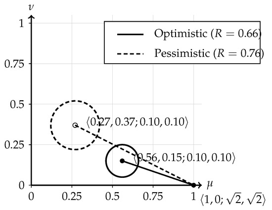
Figure 1.
Optimistic and pessimistic solutions in the plane (elliptic E-IF evaluation).
5.5.2. Algorithmic Framework
Quantitative Interpretation and Discussion
The second-stage plan allocates approximately 900–950 pallets per quarter between the three resellers and four OEM factories. After defuzzification (), the realized shipment volumes are:
The aggregated expected transportation–resale cost for the stage equals
corresponding to a mean selling margin of above the purchase cost from Stage I. Budget-limit violations () occur in less than of flows, mostly on routes with higher time dispersion (). The elliptic reliability index indicates moderate risk and acceptable stability under anisotropic uncertainty. A crisp-cost re-optimization would yield , i.e., the E-IFQ formulation saves while keeping reliability above 0.6.
Practical and Policy Implications
The presented case study demonstrates that the proposed 2-S 3-D E-IFTP model is well-suited for modern high-value and energy-intensive supply chains, such as the transportation of lithium-ion battery modules for EV manufacturing. The elliptic intuitionistic fuzzy representation captures correlated uncertainties related to fuel prices, demand fluctuations, and regulatory constraints (e.g., carbon tariffs or safety regulations). This makes the framework applicable not only to EV logistics but also to renewable-energy storage, smart manufacturing, and sustainable distribution networks requiring multi-stage, multi-period optimization under uncertainty. Thus, the case study provides both methodological validation and direct industrial relevance of the proposed approach (see Figure 2 and Algorithm 1).
| Algorithm 1 Two-Stage 3-D E-IFQ Transportation Solver |
|
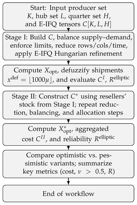
Figure 2.
Workflow of the two-stage three-dimensional E-IFQ transportation algorithm.
6. Discussion
The proposed two-stage three-dimensional transportation problem under Elliptic Intuitionistic Fuzzy Quadruples (2-S 3-D E-IFTP) establishes a flexible framework for modeling logistics systems subject to complex and correlated uncertainties. By extending the index-matrix interpretation from two to three dimensions, the model accommodates both spatial and temporal aspects of distribution networks, while explicitly incorporating the role of resellers in multi-stage flows.
The case study on EV battery module distribution illustrates the practical advantages of the E-IFQ approach. The results show that the proposed model:
- provides more robust solutions compared to classical fuzzy and intuitionistic fuzzy formulations,
- effectively captures anisotropic variability in transportation costs, demand, and supply,
- maintains feasibility under cost-limit shocks and demand fluctuations by leveraging buffer allocations, and
- delivers higher precision in ranking alternative transportation plans through the elliptic distance measure.
From a managerial standpoint, the model provides actionable insights for supply chain planners in emerging industries such as electromobility. The capability to account for correlated uncertainties—such as raw material price volatility, shipping disruptions, and environmental regulations—enhances the reliability of logistics decision-making in EV production networks. Moreover, future extensions may integrate optimized quasi-Monte Carlo sensitivity methods, similar to those proposed in [61], to further improve uncertainty quantification and computational efficiency in high-dimensional industrial environments.
7. Concluding Remarks
This study broadens the scope of fuzzy transportation research by introducing E-IFQs into a multi-stage, multi-dimensional optimization context. The findings emphasize the value of elliptic intuitionistic fuzzy modeling for addressing anisotropic uncertainty and correlated risks in modern supply chains.
Future research may focus on integrating the 2-S 3-D E-IFTP with metaheuristic solvers, hybrid optimization methods, and simulation-based analysis, as well as extending applications to other high-uncertainty domains such as renewable energy distribution, healthcare logistics, and disaster response.
Author Contributions
Conceptualization, V.T. and S.T.; methodology, V.T.; validation, V.T. and S.T.; formal analysis, V.T. and S.T.; investigation, V.T. and S.T.; resources, V.T. and S.T.; data curation, V.T. and S.T.; writing—original draft preparation, V.T. and S.T.; writing—review and editing, V.T.; supervision, V.T. and S.T.; project administration, S.T.; funding acquisition, V.T. All authors have read and agreed to the published version of the manuscript.
Funding
This research was carried out with the support of two projects: (1) the University-Wide Research Grant No. OUF-RD-15/2025, entitled “Extraction of Expert Knowledge through Innovative Analytical Methods”, funded by the BSU “Prof. Dr. Assen Zlatarov”, which supported the theoretical and methodological developments presented in Section 1, Section 2, Section 3, Section 4 and Section 5; and (2) the Project No. BG16RFPR002-1.014-0019-C01 “Establishment and Sustainable Development of a Centre of Competence in Mechatronics and Clean Technologies—MIRACle”, which supported the application, integration, and sustainability analysis discussed in Section 6 and Section 7.
Data Availability Statement
No new data were created or analyzed in this study. Data sharing is not applicable to this article.
Acknowledgments
The authors express their sincere gratitude to Stoyan Tranev for leading the University-Wide Research Grant OUF-RD-15/2025 and for his valuable methodological guidance. The authors also acknowledge the infrastructural and technical support provided by the Centre of Competence in Mechatronics and Clean Technologies “MIRACle” (Project BG16RFPR002-1.014-0019-C01).
Conflicts of Interest
The authors declare no conflicts of interest.
References
- Hitchcock, F.L. The Distribution of a Product from Several Sources to Numerous Localities. J. Math. Phys. 1941, 20, 224–230. [Google Scholar] [CrossRef]
- Dantzig, G.B. Linear Programming and Extensions; Princeton University Press: Princeton, NJ, USA, 1963. [Google Scholar]
- Kantorovich, L.V. Mathematical Methods of Organizing and Planning Production. Manag. Sci. 1960, 6, 366–422. [Google Scholar] [CrossRef]
- Zadeh, L.A. Fuzzy Sets. Inf. Control 1965, 8, 338–353. [Google Scholar] [CrossRef]
- Atanassov, K. Intuitionistic Fuzzy Sets. Fuzzy Sets Syst. 1986, 20, 87–96. [Google Scholar] [CrossRef]
- Kaur, A.; Kumar, A. A new approach for solving fuzzy transportation problems using generalized trapezoidal fuzzy numbers. Appl. Soft Comput. 2012, 12, 1201–1213. [Google Scholar] [CrossRef]
- Ebrahimnejad, A. An improved approach for solving fuzzy transportation problem with triangular fuzzy numbers. J. Intell. Fuzzy Syst. Appl. Eng. Technol. 2015, 29, 963–974. [Google Scholar] [CrossRef]
- Traneva, V. One application of the index matrices for solution of a transportation problem. Adv. Stud. Contemp. Math. 2016, 26, 703–715. [Google Scholar]
- Traneva, V.; Tranev, S. Intuitionistic Fuzzy Transportation Problem by Zero Point Method. In Proceedings of the 2020 Federated Conference on Computer Science and Information Systems, Sofia, Bulgaria, 6–9 September 2020; Ganzha, M., Maciaszek, L., Paprzycki, M., Eds.; ACSIS 21. Polish Information Processing Society: Warsaw, Poland, 2020; pp. 349–358. [Google Scholar] [CrossRef]
- Niroomand, S.; Allahviranloo, T.; Mahmoodirad, A.; Amirteimoori, A.; Mršić, L.; Samanta, S. Solving a Fully Intuitionistic Fuzzy Transportation Problem Using a Hybrid Multi-Objective Optimization Approach. Mathematics 2024, 12, 3898. [Google Scholar] [CrossRef]
- Kaur, A.; Kacprzyk, J.; Kumar, A. Fuzzy Transportation and Transshipment Problems; Studies in Fuzziness and Soft Computing; Springer: Cham, Switzerland, 2020; Volume 385. [Google Scholar]
- Atanassov, K.; Vassilev, P. Intuitionistic Fuzzy Elliptic Membership Functions. In Proceedings of the IEEE International Conference on Intelligent Systems, Sofia, Bulgaria, 4–6 September 2016; pp. 37–42. [Google Scholar]
- Atanassov, K.; Gargov, G. Interval-Valued Intuitionistic Fuzzy Sets. Fuzzy Sets Syst. 1989, 31, 343–349. [Google Scholar] [CrossRef]
- Atanassov, K.; Szmidt, E.; Kacprzyk, J. Circular Intuitionistic Fuzzy Sets. Notes Intuit. Fuzzy Sets 2010, 16, 19–26. [Google Scholar] [CrossRef]
- Traneva, V.; Tranev, S.; Todorov, V. An Elliptic Intuitionistic Fuzzy Model for Franchise Selection. In Proceedings of the Federated Conference on Computer Science and Information Systems (FedCSIS 2023), Warsaw, Poland, 17–20 September 2023; pp. 243–250. [Google Scholar]
- Chanas, S.; Kuchta, D. Fuzzy Integer Transportation Problem. Fuzzy Sets Syst. 1998, 98, 291–300. [Google Scholar] [CrossRef]
- Chanas, S.; Delgado, M.; Verdegay, J.L.; Vila, M.A. Interval and fuzzy extensions of classical transportation problems. Transp. Plan. Technol. 1993, 17, 203–218. [Google Scholar] [CrossRef]
- Jiménez, F.; Verdegay, J.L. Uncertain Linear Programming Problems. Fuzzy Sets Syst. 1998, 100, 45–57. [Google Scholar] [CrossRef]
- Liang, T.-F. Application of fuzzy linear programming to transportation planning decision problems with multiple fuzzy goals. In Proceedings of the 9th Joint International Conference on Information Sciences (JCIS 2006), Kaohsiung, Taiwan, 8–11 October 2006. [Google Scholar] [CrossRef][Green Version]
- Liu, S.T. Fuzzy Total Transportation Cost Measures for Fuzzy Solid Transportation Problem. Appl. Math. Comput. 2006, 174, 927–941. [Google Scholar] [CrossRef]
- Liu, S.T.; Kao, C. Solving Fuzzy Transportation Problems Based on Extension Principle. Eur. J. Oper. Res. 2004, 153, 661–674. [Google Scholar] [CrossRef]
- Pandian, P.; Natarajan, G. A New Algorithm for Finding a Fuzzy Optimal Solution for Fuzzy Transportation Problems. Appl. Math. Sci. 2010, 4, 79–90. Available online: https://www.m-hikari.com/ams/ams-2010/ams-1-4-2010/pandianAMS1-4-2010.pdf (accessed on 10 November 2025).
- Kaur, A.; Kumar, A. A New Method for Solving Fuzzy Transportation Problems. Appl. Math. Model. 2009, 33, 1868–1876. [Google Scholar] [CrossRef]
- Güzel, N. Fuzzy Transportation Problem with the Fuzzy Amounts and the Fuzzy Costs. World Appl. Sci. J. 2010, 8, 543–549. Available online: https://www.academia.edu/87137753/Fuzzy_Transportation_Problem_with_the_Fuzzy_Amounts_and_the_Fuzzy_Costs (accessed on 10 November 2025).
- Basirzadeh, H. A New Approach to Solve Fuzzy Transportation Problems. Appl. Math. Sci. 2012, 6, 805–813. Available online: https://www.m-hikari.com/ams/ams-2011/ams-29-32-2011/basirzadehAMS29-32-2011.pdf (accessed on 10 November 2025).
- Aggarwal, R.; Gupta, C. A Novel Algorithm for Solving Intuitionistic Fuzzy Transportation Problem via New Ranking Method. Ann. Fuzzy Math. Inform. 2014, 8, 753–768. Available online: http://www.afmi.or.kr/papers/2014/Vol-08_No-05/PDF/AFMI-8-5(753-768)-H-140227R1.pdf (accessed on 10 November 2025).
- Gani, A.; Begum, A.; Abbas, S. Intuitionistic Fuzzy Transportation Problem. Appl. Math. Sci. 2013, 7, 2487–2496. [Google Scholar] [CrossRef]
- Kathirvel, K.; Balamurugan, K. Method for Solving Unbalanced Transportation Problems Using Trapezoidal Fuzzy Numbers. Int. J. Eng. Res. Appl. 2013, 3, 2591–2596. [Google Scholar]
- Samuel, A. Edward; Venkatachalapathy, M. Modified Vogel’s Approximation Method for Fuzzy Transportation Problems. Appl. Math. Sci. 2011, 5, 1367–1372. Available online: https://www.m-hikari.com/ams/ams-2011/ams-25-28-2011/samuelAMS25-28-2011.pdf (accessed on 10 November 2025).
- Kumar, P.S.; Hussain, R.J. Computationally Simple Approach for Solving Fully Intuitionistic Fuzzy Real Life Transportation Problems. Int. J. Syst. Assur. Eng. Manag. 2016, 7, 90–101. [Google Scholar] [CrossRef]
- Jahirhussain, R.; Jayaraman, P. Fuzzy Optimal Transportation Problem by Improved Zero Suffix Method via Robust Rank Techniques. Int. J. Fuzzy Math. Syst. 2013, 3, 303–311. [Google Scholar]
- Samuel, A.E.; Venkatachalapathy, M. Improved Zero Point Method for Unbalanced Fuzzy Transportation Problems. Int. J. Pure Appl. Math. 2014, 94, 419–424. [Google Scholar] [CrossRef]
- Traneva, V.; Tranev, S. Index-Matrix Interpretation of a Two-Stage Three-Dimensional Intuitionistic Fuzzy Transportation Problem. In Recent Advances in Computational Optimization; Fidanova, S., Ed.; Studies in Computational Intelligence; Springer: Cham, Switzerland, 2022; Volume 1044, pp. 187–213. [Google Scholar] [CrossRef]
- Traneva, V.; Tranev, S. Intuitionistic Fuzzy Zero Suffix Method for Transportation Problem. In Advances in High Performance Computing; Dimov, I., Fidanova, S., Eds.; HPC 2019; Studies in Computational Intelligence; Springer: Cham, Switzerland, 2019; Volume 902, pp. 73–87. [Google Scholar]
- Torra, V. Hesitant Fuzzy Sets. Int. J. Intell. Syst. 2010, 25, 529–539. [Google Scholar] [CrossRef]
- Yager, R.R. Pythagorean Fuzzy Subsets. In Proceedings of the Joint IFSA World Congress and NAFIPS Annual Meeting, Edmonton, AB, Canada, 24–28 June 2013; pp. 57–61. [Google Scholar] [CrossRef]
- Kutlu Gündoğdu, F.; Kahraman, C. Spherical Fuzzy Sets. J. Intell. Fuzzy Syst. 2019, 36, 337–352. [Google Scholar] [CrossRef]
- Traneva, V.; Tranev, S. Circular Intuitionistic Fuzzy Model for Franchise Selection. In Proceedings of the INFUS 2022, Izmir, Turkey, 19–21 July 2022; pp. 532–544. [Google Scholar]
- Atanassov, K.; Vassilev, P.; Atanassova, V. Intuitionistic Fuzzy Sets and Some of Their So-Called Extensions. Notes Intuitionistic Fuzzy Sets 2025, 31, 372–385. [Google Scholar] [CrossRef]
- Cuong, B.C. Picture Fuzzy Sets. In Proceedings of the 2013 IEEE International Conference on Fuzzy Systems, Hyderabad, India, 7–10 July 2013; pp. 1–8. [Google Scholar]
- Jun, Y.B.; Kim, C.S.; Yang, K.O. Cubic Sets. Ann. Fuzzy Math. Inform. 2012, 4, 83–98. Available online: https://www.afmi.or.kr/papers/2012/Vol-04_No-01/AFMI-4-1(83-98)-J-111023.pdf (accessed on 10 November 2025).
- Wang, H.; Smarandache, F.; Zhang, Y.-Q.; Sunderraman, R. Single Valued Neutrosophic Sets. Multispace Multistruct. 2010, 4, 410–413. [Google Scholar]
- Nguyen, X.T.; Nguyen, V.D. Support-Intuitionistic Fuzzy Set: A New Concept for Soft Computing. Int. J. Intell. Syst. Appl. 2015, 4, 11–16. [Google Scholar] [CrossRef]
- Bharati, S.K. Trapezoidal Intuitionistic Fuzzy Fractional Transportation Problem. In Soft Computing for Problem Solving; Advances in Intelligent Systems and Computing; Springer: Singapore, 2019; Volume 817, pp. 833–842. [Google Scholar] [CrossRef]
- Nabeel, M.; Ahmed, A.; Khan, H. A Solution of Mathematical Multi-Objective Green Transportation Problems Under the Fermatean Fuzzy Environment. RAMD 2025, 2, 61–74. [Google Scholar] [CrossRef]
- Traneva, V.; Petrov, P.; Tranev, S. Elliptic Intuitionistic Fuzzy Portfolio Selection Problem (E-IFKP). In Proceedings of the 2023 Federated Conference on Computer Science and Information Systems (FedCSIS), Warsaw, Poland, 17–20 September 2023; ACSIS. Volume 37, pp. 329–336. [Google Scholar]
- Atanassov, K.; Marinov, M. Four Distances for Circular Intuitionistic Fuzzy Sets. Mathematics 2021, 9, 2021. [Google Scholar] [CrossRef]
- Atanassov, K. Intuitionistic Fuzzy Logics; Studies in Fuzziness and Soft Computing; Springer: Cham, Switzerland, 2017; Volume 351. [Google Scholar] [CrossRef]
- Atanassov, K.T.; Szmidt, E.; Kacprzyk, J. On Intuitionistic Fuzzy Pairs. Notes Intuit. Fuzzy Sets 2013, 19, 1–13. Available online: https://ifigenia.org/images/7/7f/NIFS-19-3-01-13.pdf (accessed on 10 November 2025).
- Atanassov, K. On Intuitionistic Fuzzy Sets Theory; Studies in Fuzziness and Soft Computing; Springer: Berlin/Heidelberg, Germany, 2012; Volume 283. [Google Scholar]
- Atanassov, K.T. Remark on an Intuitionistic Fuzzy Operation “Division”. Adv. Stud. Contemp. Math. 2021, 31, 395–399. Available online: https://www.kci.go.kr/kciportal/ci/sereArticleSearch/ciSereArtiView.kci?sereArticleSearchBean.artiId=ART002819664 (accessed on 10 November 2025).
- De, S.K.; Bisvas, R.; Roy, R. Some Operations on IFSs. Fuzzy Sets Syst. 2000, 114, 477–484. [Google Scholar] [CrossRef]
- Riečan, B.; Atanassov, K.T. Operation Division by n Intuitionistic Fuzzy Sets. Notes Intuit. Fuzzy Sets 2010, 16, 1–4. Available online: https://ifigenia.org/images/e/e1/NIFS-16-4-01-04.pdf (accessed on 10 November 2025).
- Szmidt, E.; Kacprzyk, J. Amount of Information and Its Reliability in the Ranking of Atanassov’s Intuitionistic Fuzzy Alternatives. In Recent Advances in Decision Making; Rakus-Andersson, E., Yager, R., Ichalkaranje, N., Jain, L.C., Eds.; Studies in Computational Intelligence; Springer: Berlin/Heidelberg, Germany, 2009; Volume 222, pp. 7–19. [Google Scholar] [CrossRef]
- Atanassov, K. Generalized Index Matrices. C. R. Acad. Bulg. Sci. 1987, 40, 15–18. [Google Scholar]
- Atanassov, K. Index Matrices: Towards an Augmented Matrix Calculus; Studies in Computational Intelligence; Springer: Cham, Switzerland, 2014; Volume 573. [Google Scholar]
- Traneva, V.; Tranev, S. Index Matrices as a Tool for Managerial Decision Making; Publishing House Union of Scientists: Sofia, Bulgaria, 2017. (In Bulgarian) [Google Scholar]
- Traneva, V.; Tranev, S.; Stoenchev, M.; Atanassov, K. Scaled Aggregation Operations over Two- and Three-Dimensional Index Matrices. Soft Comput. 2019, 22, 5115–5120. [Google Scholar] [CrossRef]
- Traneva, V.; Tranev, S. Zero Point Method for Transportation Problems with Elliptic Intuitionistic Fuzzy Matrices. In Intelligent and Fuzzy Systems. INFUS 2025; Kahraman, C., Cebi, S., Oztaysi, B., Cevik Onar, S., Tolga, C., Ucal Sari, I., Otay, I., Eds.; Lecture Notes in Networks and Systems; Springer: Cham, Switzerland, 2025; Volume 1528, pp. 229–238. [Google Scholar]
- Traneva, V.; Tranev, S. Circular Intuitionistic Fuzzy Index-Matrix Model for Transportation Problem. In Proceedings of the FedCSIS 2022, Sofia, Bulgaria, 4–7 September 2022; pp. 231–238. [Google Scholar]
- Todorov, V.; Dimov, I.; Ostromsky, T.; Zlatev, Z.; Georgieva, R.; Poryazov, S. Optimized Quasi-Monte Carlo Methods Based on Van der Corput Sequence for Sensitivity Analysis in Air Pollution Modelling. In Recent Advances in Computational Optimization; Fidanova, S., Ed.; Studies in Computational Intelligence; Springer: Cham, Switzerland, 2022; Volume 986, pp. 389–405. [Google Scholar]


Disclaimer/Publisher’s Note: The statements, opinions and data contained in all publications are solely those of the individual author(s) and contributor(s) and not of MDPI and/or the editor(s). MDPI and/or the editor(s) disclaim responsibility for any injury to people or property resulting from any ideas, methods, instructions or products referred to in the content. |
© 2025 by the authors. Licensee MDPI, Basel, Switzerland. This article is an open access article distributed under the terms and conditions of the Creative Commons Attribution (CC BY) license (https://creativecommons.org/licenses/by/4.0/).