On Distance Laplacian Energy of Unicyclic and Bicyclic Graphs

Abstract

For a connected graph G, let $D^L\left(G\right)$ be its distance Laplacian matrix and ${\lambda }_1\left(G\right)\ge {\lambda }_2\left(G\right)\ge \dots \ge {\lambda }_{n-1}\left(G\right)>{\lambda }_n\left(G\right)=0$ be its $D^L$ eigenvalues. The $D^L$ energy of G is defined as $DLE\left(G\right)={\sum }_{i=1}^n\left|{\lambda }_i\left(G\right)-{\displaystyle \frac{2W\left(G\right)}{n}}\right|$, where $W\left(G\right)$ is the Wiener index of G. An important problem in graph energy studies is to determine exact formulations of the energy for specific graph classes and their complements. This paper gives the precise $D^L$ energy formulations of a class of bicyclic graphs $C_2(p,q)$, a class of unicyclic graphs $C_1(p,q)$, and their complements. Moreover, we order the graphs $C_2(p,q)$ on the basic of ${\lambda }_1$, ${\lambda }_{n-1}$, and consider the same problems for their complements. And the ordering of the graphs $C_1(p,q)$ on the basic of ${\lambda }_{n-1}$ and the ordering of their complements on the basics of ${\lambda }_1$, ${\lambda }_{n-1}$ and the $D^L$ energy are obtained.

1. Introduction

The present work considers only undirected, simple and connected graphs. Let G be a connected graph, where $V\left(G\right)$ represents its vertex set and $E\left(G\right)$ represents its edge set. The distance between two vertices $u,v\in V\left(G\right)$, denoted as $d_{uv}\left(G\right)$ or simply $d_{uv}$, is the length of the shortest path linking them in G. The distance matrix $D\left(G\right)$ of G is given by $D\left(G\right)={\left(d_{uv}\right)}_{u,v\in V\left(G\right)}$. The transmission $T{r}_G\left(v\right)$ of a vertex $v\in V\left(G\right)$ is defined as the sum of distances from v to all other vertices in G, i.e., $T{r}_G\left(v\right)={\sum }_{u\in V\left(G\right)}{d}_{uv}$. Note that $T{r}_G\left(v\right)$ corresponds to the $v^{th}$ row sum of the matrix $D\left(G\right)$. The distance Laplacian matrix of G is defined as $D^L\left(G\right)=Tr\left(G\right)-D\left(G\right)$, where $Tr\left(G\right)$ is the diagonal matrix whose entries are the vertex transmissions in G. Clearly, $D^L\left(G\right)$ is a real symmetric positive semidefinite matrix. The eigenvalues of $D^L\left(G\right)$ often follow the order ${\lambda }_1\left(G\right)\ge {\lambda }_2\left(G\right)\ge \dots \ge {\lambda }_{n-1}\left(G\right)>{\lambda }_n\left(G\right)=0$ with ${\lambda }_1\left(G\right)$ and ${\lambda }_{n-1}\left(G\right)$ respectively denoted as the $D^L$ spectral radius and the second smallest $D^L$ eigenvalue of graph G. And the multiset comprising the eigenvalues of $D^L\left(G\right)$ is referred to as the $D^L$ spectrum of G.

Graph energy, a concept originating from theoretical chemistry, was first defined by Gutman [1] in 1978. When considering a simple graph G, its energy $E\left(G\right)$ is computed as the sum of the absolute values of the eigenvalues of the adjacency matrix corresponding to G. For recent advancements regarding $E\left(G\right)$, one may refer to [2,3,4,5]. Graph energy’s concept has been generalized to meet various application needs, which involves considering other matrices associated with a graph. For example, distance energy, distance signless Laplacian energy and Laplacian energy. We may refer to [6,7,8] for some of the latest progress on them. Let G denote a graph of order n. The $Wiener$ $index$ $W\left(G\right)$ of G is the sum of distances between all unordered vertex pairs, given by $W\left(G\right)={\sum }_{1\le i<j\le n}d\left(v_i,v_j\right)={\displaystyle \frac{1}{2}}{\sum }_{v\in V\left(G\right)}T{r}_G\left(v\right)$. In 2013, Yang, You and Gutman [9] defined $DLE\left(G\right)={\sum }_{i=1}^n\left|{\lambda }_i\left(G\right)-{\displaystyle \frac{2W\left(G\right)}{n}}\right|$. One of the interesting questions concerning the study of the energy of the graph is to give the upper and lower bounds of the energy. Yang, You and Gutman [9] gave some bounds on $DLE\left(G\right)$ for a simple connected graph. Das, Aouchiche and Hansen [6] presented some bounds on $DLE\left(G\right)$ in terms of n for some graphs. Diaz and Rojo [7] gave the sharp upper bound on $DLE\left(G\right)$ energy for a simple undirected connected graph. Moreover, another problem of concern is to characterize the distinct energy formulation of a given graph class. The complement graph of a graph $G=(V,E)$, denoted by $\overline{G}$, is a graph whose vertex set is same to that of G, but two vertices in $\overline{G}$ are adjacent if and only if they are not adjacent in G. Rather, Aouchiche, Imran and Ei Hallaoui [10] provided $DLE\left(G\right)$ energy of the graphs whose complements are double stars, as well as for a specific type of unicyclic graph and their complements. Rather, Ganie and Shang [11] derived $DLE\left(G\right)$ energy of sun and partial sun graphs. Determining exact distance Laplacian energy expression for key graph classes is significant, as it aids in addressing various extremal problems in spectral graph theory. In the course of previous research, we have found that Figure 1 have an important place in the extremal graph theory. Compared to [10,11,12], the $D^L$ energy formulations described in this paper is more specific. In addition, Our process of calculating $DLE$ is also more complex. Motivated by the aforementioned studies, the central objective of this paper is stated in Problem 1.

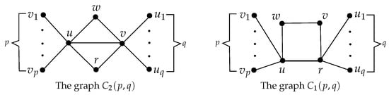
Problem 1.

Can we determine $DLE\left(G\right)$ for two types of graphs in Figure 1 and their complements?

Let $C_4=uwvru$ be a cycle. The graph $C_2(p,q)$ (see Figure 1) is obtained by inserting an edge connecting vertices u and v within the $C_4$ and attaching p and q pendent vertices to vertices u and v, respectively. The graph $C_1(p,q)$ (see Figure 1) is constructed by appending p and q pendent vertices to vertices u and r of the $C_4$ cycle, respectively. Obviously, the graphs $C_2(p,q)$ and $C_1(p,q)$ are a bicyclic graph and an unicyclic graph, respectively. Then we answer the Problem 1 based on the graphs $C_2(p,q)$ and $C_1(p,q)$.

Theorem 1.

Let G be a graph of order $n=p+q+4$ such that $G\cong C_2(p,q)$, where $p\ge q\ge 1$. Let ${\lambda }_1\ge {\lambda }_2\ge \dots \ge {\lambda }_{n-1}>{\lambda }_n=0$ be the $D^L$ eigenvalues of G. Then ${\lambda }_1\in \left(3p+3q+7,3p+3q+8\right)$ and ${\lambda }_{n-4}\in \left(2p+2q+6+{\displaystyle \frac{1}{p+q+4}},2p+2q+7\right)$. Furthermore, The following properties are satisfied:

(i) 

If $1\le pq\le n+1$, then

$$DLE\left(G\right)=2\left({\lambda }_1+{\lambda }_{n-4}-{\displaystyle \frac{2p^2-2pq+2q^2+18p+18q+46}{p+q+4}}\right).$$

(ii) 

If $n+1<pq<{\displaystyle \frac{3n}{2}}+1$, then

$$DLE\left(G\right)=\left\{\begin{array}{cc}2\left({\lambda }_1+{\displaystyle \frac{10pq-8p-8q-42}{p+q+4}}\right),\hfill & if{\lambda }_{n-4}\in I_1,\hfill \\ 2\left({\lambda }_1+{\lambda }_{n-4}-{\displaystyle \frac{2p^2+2q^2-4pq+20p+20q+56}{p+q+4}}\right),\hfill & if{\lambda }_{n-4}\in I_2,\hfill \end{array}\right.$$

where

$$I_1=\left(2p+2q+6+{\displaystyle \frac{1}{p+q+4}},{\displaystyle \frac{2p^2+2q^2+6pq+12p+12q+14}{p+q+4}}\right),$$

$$I_2=\left[{\displaystyle \frac{2p^2+2q^2+6pq+12p+12q+14}{p+q+4}},2p+2q+7\right).$$

(iii) 

If ${\displaystyle \frac{3n}{2}}+1\le pq\le 3n+q^2+4q+2$, then

$$DLE\left(G\right)=2\left({\lambda }_1+{\displaystyle \frac{10pq-8p-8q-42}{p+q+4}}\right).$$

(iv) 

If $pq>3n+q^2+4q+2$, then

$$DLE\left(G\right)=2\left({\lambda }_1+{\displaystyle \frac{p^{2}q-p{q}^2-3p^2+2pq+q^2-19p-q-28}{p+q+4}}\right).$$

Theorem 2.

Let G be a graph of order $n=p+q+4$ such that $G\cong \overline{C_2(p,q)}$, where $p\ge q\ge 1$. Let ${\lambda }_1\ge {\lambda }_2\ge \dots \ge {\lambda }_{n-1}>{\lambda }_n=0$ be the $D^L$ eigenvalues of G. Then ${\lambda }_{n-1}\in \left(n,n+1\right)$. Furthermore, the following statements hold:

(i) 

If ${\lambda }_4\in \left(n+1,n+1+{\displaystyle \frac{4}{n}}\right)$, then

$$DLE\left(G\right)=2\left({\displaystyle \frac{3p^2+3q^2+6pq+31q+31p+64}{p+q+4}}-{\lambda }_4-{\lambda }_{n-1}\right).$$

(ii) 

If ${\lambda }_4\in \left[n+1+{\displaystyle \frac{4}{n}},n+2-{\displaystyle \frac{1}{n}}\right)$, then

$$DLE\left(G\right)=2\left({\displaystyle \frac{2p^2+4pq+2q^2+22p+22q+40}{p+q+4}}-{\lambda }_{n-1}\right).$$

Theorem 3.

Let G be a graph of order $n=p+q+4$ such that $G\cong C_1(p,q)$, where $p\ge q\ge 1$. Then, $D^L$ spectrum of the graph G comprises the eigenvalue $3q+2p+8$ occurring with multiplicity $p-1$, the eigenvalue $3p+2q+8$ occurring with multiplicity $q-1$, a single instance of the eigenvalue 0, and the eigenvalue $z_i$ for $0\le i\le 4$, where $z_0\in \left(3p+3q+8,3p+3q+10\right)$, $z_1\in \left(3p+2q+6,3p+2q+8\right]$ and $z_2\in \left[2p+2q+6,3p+2q+6\right)$. Furthermore, the following statements hold:

(i) 

If $1\le pq\le 4$, then

$$DLE\left(G\right)=2\left(z_0+z_1+z_2-{\displaystyle \frac{5p^2+4pq+5q^2+34p+34q+80}{p+q+4}}\right).$$

(ii) 

If $4<pq\le q^2+2p+6q+6$, then

$$DLE\left(G\right)=\left\{\begin{array}{cc}2\left(z_0+z_1-{\displaystyle \frac{3p^2-2pq+3q^2+20p+20q+64}{p+q+4}}\right),\hfill & if{z}_2\in I_1,\hfill \\ 2\left(z_0+z_1+z_2-{\displaystyle \frac{5p^2+4pq+5q^2+34p+34q+80}{p+q+4}}\right),\hfill & if{z}_2\in I_2,\hfill \end{array}\right.$$

where

$$I_1=\left[2p+2q+6,{\displaystyle \frac{2p^2+6pq+2q^2+14p+14q+16}{p+q+4}}\right),$$

$$I_2=\left[{\displaystyle \frac{2p^2+6pq+2q^2+14p+14q+16}{p+q+4}},3p+2q+6\right).$$

(iii) 

If $pq>q^2+2p+6q+6$, then

$$DLE\left(G\right)=\left\{\begin{array}{cc}2\left(z_0+z_1+{\displaystyle \frac{(p+2)(pq-q^2-5p-7q-24)}{p+q+4}}\right),\hfill & if{z}_2\in I_1,\hfill \\ 2\left(z_0+z_1+z_2+{\displaystyle \frac{p^{2}q-p{q}^2-7p^2-11pq-4q^2-48p-28q-64}{p+q+4}}\right),\hfill & if{z}_2\in I_2,\hfill \end{array}\right.$$

where

$$I_1=\left[2p+2q+6,{\displaystyle \frac{2p^2+6pq+2q^2+14p+14q+16}{p+q+4}}\right),$$

$$I_2=\left[{\displaystyle \frac{2p^2+6pq+2q^2+14p+14q+16}{p+q+4}},3p+2q+6\right).$$

Remark 1.

We give $DLE\left(C_1(p,q)\right)$, $DLE(\overline{C_1(p,q))}$, $DLE\left(C_2(p,q)\right)$ and $DLE\left(\overline{C_2(p,q)}\right)$ in this article. In particular, $DLE(\overline{C_1(p,q)}$) will be presented in the form of Corollary 9, based on some previous results in the last section.

Additionally, ordering graphs of the same order according to a given spectral invariant remains a key direction in current research. Ganie [13] demonstrated that trees with a diameter of 3 are distinguishable based on their $D^L$ energy. Rather, Ganie and Shang [11] ordered sun and partial sun graphs by using their $D^L$ energies. And they also ordered them on the basic of ${\lambda }_1$ and ${\lambda }_{n-1}$. Rather, Aouchiche, Imran and Ei Hallaoui [10] ordered the graphs whose complements are double stars on the basic of ${\lambda }_1$ and ${\lambda }_{n-1}$ and a special type of unicyclic graph and their complements on the basic of ${\lambda }_1$ and ${\lambda }_{n-1}$. Therefore, this paper also orders part of the graphs mentioned above on the basic of ${\lambda }_1$, ${\lambda }_{n-1}$ and the $D^L$ energy.

The structure of the paper is as follows: In Section 2, we order the graphs $C_2(p,q)$ and $\overline{C_2(p,q)}$ by their ${\lambda }_1$ and ${\lambda }_{n-1}$, respectively, and discuss their $DLE$. Section 3 presents $DLE\left(C_1(p,q)\right)$ and $DLE\left(\overline{C_1(p,q)}\right)$. Additionally, we examine the ordering of $C_1(p,q)$ graphs with respect to ${\lambda }_{n-1}$. And we also order the graphs $\overline{C_1(p,q)}$ on the basic of ${\lambda }_1$, ${\lambda }_{n-1}$ and the $D^L$ energy.

2. Proof of Theorems 1 and 2

Let G be a graph whose vertex set is given by $V\left(G\right)=\{v_1,\dots ,v_n\}$. In this context, $X={(x_1,\dots ,x_n)}^T\in {\mathbb{R}}^n$ represents a function (or mapping) defined over $V\left(G\right)$, where each vertex $v_i$ is assigned a corresponding value $x_i$ for $i=1,\dots ,n$. Additionally, it is given that

$$X^T{D}^L\left(G\right)X=\sum _{\left\{u,v\right\}\subseteq V\left(G\right)}{d}_{uv}{\left(x_u-x_v\right)}^2,$$

and $\lambda$ serves as an eigenvalue of $D^L\left(G\right)$, associated with the eigenvector X if and only if for all vertices $v\in V\left(G\right)$,

$$\lambda x_v=\sum _{u\in V\left(G\right)}{d}_{uv}\left(x_v-x_u\right),$$

or equivalently,

$$\lambda x_v=Tr\left(v\right)x_v-\sum _{u\in V\left(G\right)}{d}_{uv}{x}_u.$$

(1)

Let $N_G\left(v\right)=\{u\mid uv\in E\left(G\right)\}$. Let $S\subseteq V\left(G\right)$ and $G\left[S\right]$ denote an induced subgraph on a vertex subset S. A vertex subset S is termed an independent set of G if $G\left[S\right]=\left|S\right|K_1$.

Lemma 1

([14]). Consider a graph G with n vertices. Suppose $S=\left\{v_1,v_2,\dots ,v_p\right\}$ is an independent set in G such that $N\left(v_i\right)=N\left(v_j\right)$ for all $i,j\in \left\{1,\dots ,p\right\}$, then $\theta =Tr\left(v_i\right)=Tr\left(v_j\right)$ for all $i,j\in \left\{1,\dots ,p\right\}$ and $\theta +2$ is an eigenvalues of $D^L\left(G\right)$ with multiplicity $\mathcal{N}\ge p-1$.

Let

$$M={\left(\begin{array}{cccc}{A}_{11}& A_{12}& \dots & A_{1s}\\ A_{21}& A_{22}& \dots & A_{2s}\\ ⋮& ⋮& \ddots & ⋮\\ A_{s1}& A_{s2}& \dots & A_{ss}\end{array}\right)}_{n\times n},$$

which is devided by a partition $\Pi =\left\{{\Pi }_1,{\Pi }_2,\dots ,{\Pi }_s\right\}$ of set $\Omega =\left\{1,2,\dots ,n\right\}$. Let $Q={\left(k_{ij}\right)}_{s\times s}$ be a quotient matrix, where its $(i,j)$-th entry of the matrix is defined as the mean row sum of the submatrix $A_{ij}$ obtained from M. A partition $\Pi$ of matrix A is called equitable (or regular) if each submatrix $A_{ij}$ induced by $\Pi$ has uniform row sums across all rows for every pair of indices i and j. When this condition holds, Q is referred to as the equitable quotient matrix. The eigenvalues of Q exhibit an interlacing relationship with those of M; however, in the case of equitable partitions, the spectrum of Q forms a subset of the spectrum of M. Let $\mathsf{\Sigma }$ denote the largest positive integer for which ${\lambda }_{\mathsf{\Sigma }}\ge {\displaystyle \frac{2W\left(G\right)}{n}}$ and define $S_k\left(G\right)={\sum }_{i=1}^k{\lambda }_i$ enote the partial eigenvalue sum of the k largest values in the spectrum of $D^L$ for graph G. Given the established fact [6] that ${\sum }_{i=1}^n{\lambda }_i=2W\left(G\right)$, it can be deduced that

$$DLE\left(G\right)=2\left(S_{\Sigma }\left(G\right)-{\displaystyle \frac{2\Sigma W\left(G\right)}{n}}\right)=2\underset{1\le j\le n}{max}\left(\sum _{i=1}^j{\lambda }_i\left(G\right)-{\displaystyle \frac{2jW\left(G\right)}{n}}\right).$$

Proof of Theorem 1. 

Recall that

$$V\left(C_2\left(p,q\right)\right)=\left\{u,v,w,r,v_1,v_2,\dots ,v_p,u_1,u_2,\dots ,u_q\right\}.$$

Note that $T_r\left(v_i\right)=2p+3q+5$ for $1\le i\le p$. Thus, $2p+3q+7$ serves as a $D^L$ eigenvalue of $C_2\left(p,q\right)$ with a multiplicity of no less than $p-1$ by Lemma 1. Likewise, $3p+2q+7$ is the $D^L$ eigenvalue of $C_2\left(p,q\right)$ with a multiplicity of no less than $q-1$. Next, we will determine the remaining $D^L$ eigenvalues for $C_2\left(p,q\right)$. Let X denote the eigenvector of $C_2\left(p,q\right)$ such that $x_v=X\left(v\right)$ for $v\in V\left(G\right)$. Let $X\left(v_i\right)=x_1$ for $1\le i\le p$ and $X\left(u_i\right)=x_5$ for $1\le i\le q$ by symmetry. For the convenience of subsequent use, we set $X\left(u\right)=x_2$, $X\left(v\right)=x_4$, $X\left(w\right)=x_3$ and $X\left(r\right)=x_6$. By using the Equation (1), we have

$$\begin{array}{cc}\hfill \lambda x_1& =\left(3q+7\right)x_1-x_2-2x_3-2x_4-3q{x}_5-2x_6,\hfill \\ \hfill \lambda x_2& =-p{x}_1+\left(2q+p+3\right)x_2-x_3-x_4-2q{x}_5-x_6,\hfill \\ \hfill \lambda x_3& =-2p{x}_1-x_2+\left(2p+2q+4\right)x_3-x_4-2q{x}_5-2x_6,\hfill \\ \hfill \lambda x_4& =-2p{x}_1-x_2-x_3+\left(2p+q+3\right)x_4-q{x}_5-x_6,\hfill \\ \hfill \lambda x_5& =-3p{x}_1-2x_2-2x_3-x_4+\left(3p+7\right)x_5-2x_6,\hfill \\ \hfill \lambda x_6& =-2p{x}_1-x_2-2x_3-x_4-2q{x}_5+\left(2p+2q+4\right)x_6.\hfill \end{array}$$

Let ${\lambda }_1\ge {\lambda }_2\ge \dots \ge {\lambda }_{n-1}>{\lambda }_n=0$ represent the $D^L$ eigenvalues of graph $C_2\left(p,q\right)$. The coefficient matrix (also referred to as the regular quotient matrix of $C_2\left(p,q\right)$) corresponding to the right-hand side of the aforementioned eigenvalue equation is

$$\left[\begin{array}{cccccc}3q+7& -1& -2& -2& -3q& -2\\ -p& 2q+p+3& -1& -1& -2q& -1\\ -2p& -1& 2p+2q+4& -1& -2q& -2\\ -2p& -1& -1& 2p+q+3& -q& -1\\ -3p& -2& -2& -1& 3p+7& -2\\ -2p& -1& -2& -1& -2q& 2p+2q+4\end{array}\right]$$

and its characteristic polynomial is $\lambda f(\lambda ,p,q)$, where $f(\lambda ,p,q)={\lambda }^5-(10p+10q+28){\lambda }^4+(39p^2+79pq+39q^2+221p+221q+309){\lambda }^3-(74p^3+229p^{2}q+229p{q}^2+74q^3+637p^2+1296pq+637q^2+1803p+1803q+1678){\lambda }^2+(68p^4+288p^{3}q+440p^2{q}^2+288p{q}^3+68q^4+792p^3+2476p{q}^2+792q^3+3410p^2+6972pq+3410q^2+6430q+6430p+4480)\lambda -(24p^5+132p^{4}q+276p^3{q}^2+276p^2{q}^3+132p{q}^4+24q^5+356p^4+1536p^{3}q+2360p^2{q}^2+1536p{q}^3$$+356q^4+2080p^3+6580p^{2}q+6580p{q}^2+2080q^3+5980p^2+12296pq+5980q^2+8456p+8456q+4704)$. Note that

$$f(p+q+4,p,q)=-2pq(q+4+p)(q+2+p)(q+1+p)<0,$$

$$f(2p+q+4,p,q)=pq(q+2)(-q+p+1)>0,$$

$$f(2p+2q+4,p,q)=-4pq(q+4+p)<0,$$

$$f(2p+2q+6,p,q)=0,$$

$$f(2p+2q+6+{\displaystyle \frac{1}{p+q+4}},p,q)={\displaystyle \frac{1}{{(p+q+4)}^5}}g(p,q)>0,$$

$$f(2p+2q+7,p,q)=-pq(p+q+7)<0,$$

$$f(3p+3q+7,p,q)=-pq(3p+3q+7)(q+1+p)<0,$$

$$f(3p+3q+8,p,q)=2(q+4+p)(q+2+p)(p^2+pq+q^2+3p+3q+2)>0,$$

where $g(p,q)=2p^6+7p^{5}q+10p^4{q}^2+10p^3{q}^3+10p^2{q}^4+7p{q}^5+2q^6+37p^5+105p^{4}q+130p^3{q}^2$$+130p^2{q}^3+105p{q}^4+37q^5+276p^4+625p^{3}q+698p^2{q}^2+625p{q}^3+276q^4+1053p^3+1887p^{2}q+1887p{q}^2+1053q^3+2133p^2+3002pq+2133q^2+2106p+2106q+729$. Consequently, through the application of the intermediate value theorem along with a straightforward analysis, we can deduce that

$${\lambda }_1\in \left(3p+3q+7,3p+3q+8\right),$$

$${\lambda }_{n-4}\in \left(2p+2q+6+{\displaystyle \frac{1}{p+q+4}},2p+2q+7\right),$$

$${\lambda }_{n-3}=2p+2q+6,$$

$${\lambda }_{n-2}\in \left(2p+q+4,2p+2q+4\right),$$

$${\lambda }_{n-1}\in \left(p+q+4,2p+q+4\right).$$

In the following, we proceed to compute $DLE\left(C_2\left(p,q\right)\right)$ according to its definition. For $p\ge q\ge 1$, the mean of the $D^L$ eigenvalues for $C_2\left(p,q\right)$ is

$${\displaystyle \frac{W\left(C_2\left(p,q\right)\right)}{n}}={\displaystyle \frac{p^2+q^2+3pq+6p+6q+7}{p+q+4}}.$$

Note that ${\lambda }_1>{\displaystyle \frac{2W\left(C_2\left(p,q\right)\right)}{n}}$, ${\lambda }_{n-2}<{\displaystyle \frac{2W\left(C_2\left(p,q\right)\right)}{n}}$ and ${\lambda }_{n-1}<{\displaystyle \frac{2W\left(C_2\left(p,q\right)\right)}{n}}$. If $3p+2q+7<{\displaystyle \frac{2W\left(C_2\left(p,q\right)\right)}{n}}$, then $p^2-pq+7p+3q+14=p\left(p-q\right)+7p+3q+14<0$, a contradiction. Then, we suppose that ${\lambda }_{n-3}=2p+2q+6\ge {\displaystyle \frac{2W\left(C_2\left(p,q\right)\right)}{n}}$. It implies that $pq\le p+q+5$. Therefore, we can obtain ${\lambda }_{n-4}>{\displaystyle \frac{2W\left(C_2\left(p,q\right)\right)}{n}}$ and $2p+3q+7>{\displaystyle \frac{2W\left(C_2\left(p,q\right)\right)}{n}}$. Thus, $\mathsf{\Sigma }=q+p+1$. And the $DLE\left(C_2\left(p,q\right)\right)$ is

$$\begin{array}{cc}\hfill DLE\left(C_2\left(p,q\right)\right)=2& \left(\sum _{i=1}^{q+p+1}{\lambda }_i-{\displaystyle \frac{2\left(q+p+1\right)W\left(C_2\left(p,q\right)\right)}{n}}\right)\hfill \\ \hfill =2& \left((2p+3q+7)(p-1)+(3p+2q+7)(q-1)+\right.\hfill \\ \hfill & {\lambda }_1+{\lambda }_{n-4}+2p+2q+6-\hfill \\ \hfill & \left.{\displaystyle \frac{(q+p+1)(2p^2+2q^2+6pq+12p+12q+14)}{q+p+4}}\right)\hfill \\ \hfill =2& \left({\lambda }_1+{\lambda }_{n-4}-{\displaystyle \frac{2p^2-2pq+2q^2+18p+18q+46}{q+p+4}}\right).\hfill \end{array}$$

If $pq>q+p+5$, then ${\lambda }_{n-3}=2p+2q+6<{\displaystyle \frac{2W\left(C_2\left(p,q\right)\right)}{n}}$. Next, we compare the upper bound of ${\lambda }_{n-4}$. Now, we assume that $2p+2q+7>{\displaystyle \frac{2W\left(C_2\left(p,q\right)\right)}{n}}$. Then we get that $2p+3q+7>{\displaystyle \frac{2W\left(C_2\left(p,q\right)\right)}{n}}$, $3p+2q+7>{\displaystyle \frac{2W\left(B\left(p,q\right)\right)}{n}}$ and $pq<{\displaystyle \frac{3p}{2}}+{\displaystyle \frac{3q}{2}}+7$. For $p+q+5<pq<{\displaystyle \frac{3p}{2}}+{\displaystyle \frac{3q}{2}}+7$, ${\lambda }_{n-4}\in (2q+2p+6+{\displaystyle \frac{1}{q+p+4}},2p+2q+7)$. If ${\lambda }_{n-4}\in \left(2q+2p+6+{\displaystyle \frac{1}{q+p+4}},{\displaystyle \frac{2W\left(C_2\left(p,q\right)\right)}{n}}\right)$, then $\mathsf{\Sigma }=q+p-1$. And the $DLE\left(C_2\left(p,q\right)\right)$ is

$$\begin{array}{cc}\hfill DLE\left(C_2\left(p,q\right)\right)=& 2\left(\sum _{i=1}^{q+p-1}{\lambda }_i-{\displaystyle \frac{2\left(q+p-1\right)W\left(C_2\left(p,q\right)\right)}{n}}\right)\hfill \\ \hfill =& 2\left((2p+3q+7)(p-1)+(3p+2q+7)(q-1)+{\lambda }_1\right.\hfill \\ \hfill & -{\displaystyle \frac{(p+q-1)(2p^2+2q^2+6pq+12p+12q+14)}{q+p+4}})\hfill \\ \hfill =& 2\left({\lambda }_1+{\displaystyle \frac{10pq-8p-8q-42}{q+p+4}}\right).\hfill \end{array}$$

If ${\lambda }_{n-4}\in \left[{\displaystyle \frac{2W\left(C_2\left(p,q\right)\right)}{n}},2p+2q+7\right)$. then $\mathsf{\Sigma }=q+p$. And the $DLE\left(C_2\left(p,q\right)\right)$ is

$$\begin{array}{cc}\hfill DLE\left(C_2\left(p,q\right)\right)=& 2\left(\sum _{i=1}^{q+p}{\lambda }_i-{\displaystyle \frac{2\left(p+q\right)W\left(C_2\left(p,q\right)\right)}{n}}\right)\hfill \\ \hfill =& 2\left((2p+3q+7)(p-1)+(3p+2q+7)(q-1)\right.\hfill \\ \hfill & +{\lambda }_1+{\lambda }_{n-4}-{\displaystyle \frac{(p+q)(2p^2+2q^2+6pq+12p+12q+14)}{q+p+4}})\hfill \\ \hfill =& 2\left({\lambda }_1+{\lambda }_{n-4}-{\displaystyle \frac{2p^2+2q^2-4pq+20p+20q+56}{q+p+4}}\right).\hfill \end{array}$$

If $q^2+3p+7q+14\ge pq\ge {\displaystyle \frac{3p}{2}}+{\displaystyle \frac{3q}{2}}+7$, then $3p+2q+7\ge {\displaystyle \frac{2W\left(C_2\left(p,q\right)\right)}{n}}$, $2p+3q+7\ge {\displaystyle \frac{2W\left(C_2\left(p,q\right)\right)}{n}}$ and ${\lambda }_1>{\displaystyle \frac{2W\left(C_2\left(p,q\right)\right)}{n}}$. Thus, $\mathsf{\Sigma }=q+p-1$. And the $DLE\left(C_2\left(p,q\right)\right)$ is

$$\begin{array}{cc}\hfill DLE\left(C_2\left(p,q\right)\right)=& 2\left(\sum _{i=1}^{q+p-1}{\lambda }_i-{\displaystyle \frac{2\left(p+q-1\right)W\left(C_2\left(p,q\right)\right)}{n}}\right)\hfill \\ \hfill =& 2\left((2p+3q+7)(p-1)+(3p+2q+7)(q-1)+{\lambda }_1\right.\hfill \\ \hfill & -{\displaystyle \frac{(p+q-1)(2p^2+2q^2+6pq+12p+12q+14)}{q+p+4}})\hfill \\ \hfill =& 2\left({\lambda }_1+{\displaystyle \frac{10pq-8p-8q-42}{q+p+4}}\right).\hfill \end{array}$$

If $pq>q^2+3p+7q+14$, then $3p+2q+7\ge {\displaystyle \frac{2W\left(C_2\left(p,q\right)\right)}{n}}$ and ${\lambda }_1>{\displaystyle \frac{2W\left(C_2\left(p,q\right)\right)}{n}}$. Hence, $\Sigma =q-1+1=q$. And the $DLE\left(C_2\left(p,q\right)\right)$ is

$$\begin{array}{cc}\hfill DLE\left(C_2\left(p,q\right)\right)=& 2\left(\sum _{i=1}^q{\lambda }_i-{\displaystyle \frac{2qW\left(B\left(p,q\right)\right)}{n}}\right)\hfill \\ \hfill =& 2\left((3p+2q+7)(q-1)+{\lambda }_1\right.\hfill \\ \hfill & -{\displaystyle \frac{q(2p^2+2q^2+6pq+12p+12q+14)}{p+q+4}})\hfill \\ \hfill =& 2\left({\lambda }_1+{\displaystyle \frac{p^{2}q-p{q}^2-3p^2+2pq+q^2-19p-q-28}{p+q+4}}\right)\hfill \end{array}$$

□

Next, we give an example for Theorem 1 in the

Table 1. The $D^L$ energies of the graphs $C_2(p,q)$.

${\mathit{C}}_2(2,2)$	${\mathit{C}}_2(4,4)$	${\mathit{C}}_2(8,2)$	${\mathit{C}}_2(6,6)$	${\mathit{C}}_2(60,4)$
36.06	71.52	80.47	114.31	455.93

.

Corollary 1.

Let p and q be two positive integers, and $p\ge q\ge 2$. Consider the equation $q+p+4=n$, the following holds

$${\lambda }_1\left(C_2\left(p,q\right)\right)>{\lambda }_1\left(C_2\left(p+1,q-1\right)\right).$$

Proof. 

For Theorem 1, ${\lambda }_1\left(C_2\left(p,q\right)\right)$ denotes the maximum root of the equation $f(\lambda ,p,q)=0$. Through direct computation, it can be shown that

$$f\left(\lambda ,p,q\right)-f\left(\lambda ,p+1,q-1\right)=\left(p-q+1\right)\left(\lambda -2q-2q-6\right)g\left(\lambda \right),$$

where $g\left(x\right)={\lambda }^2-5\lambda p-5\lambda q+6p^2+12pq+6q^2-16\lambda +38p+38q+56$. By Theorem 1, ${\lambda }_1\left(C_2\left(p,q\right)\right)>3p+3q+7$. Also, $g^{\prime }\left(\lambda \right)=2x-5p-5q-16>g^{\prime }(3p+3q+7)=p+q-2\ge 0$. Thus $g\left(\lambda \right)$ is a monotonically increasing function for $\lambda$ and $g\left(\lambda \right)\le g(3p+3q+8)=-2q-2q-8<0$. Therefore, $f\left(\lambda ,p,q\right)-f\left(\lambda ,p+1,q-1\right)<0$. Note that $f({\lambda }_1\left(C_2\left(p,q\right)\right),p,q)=0$ and $f({\lambda }_1\left(C_2\left(p,q\right)\right),p+1,q-1)>0$. It implies that

$${\lambda }_1\left(C_2\left(p,q\right)\right)>{\lambda }_1\left(C_2\left(p+1,q-1\right)\right).$$

□

Applying Corollary 1 directly yields the subsequent conclusion.

Corollary 2.

Let p and q be two positive integers, and $p\ge q\ge 2$. Consider the equation $q+p+4=n$, the following holds

$${\lambda }_1\left(C_2\left(\lceil {\displaystyle \frac{n-4}{2}}\rceil ,\lfloor {\displaystyle \frac{n-4}{2}}\rfloor \right)\right)>{\lambda }_1\left(C_2\left(p+1,q-1\right)\right)>\dots >{\lambda }_1\left(C_2\left(n-5,1\right)\right).$$

Similarly, we can obtain the following result for ${\lambda }_{n-1}\left(C_2(p,q)\right)$.

Corollary 3.

Let p and q be two positive integers, and $p\ge q\ge 2$. Consider the equation $q+p+4=n$, the following holds

$${\lambda }_{n-1}\left(C_2\left(\lceil {\displaystyle \frac{n-4}{2}}\rceil ,\lfloor {\displaystyle \frac{n-4}{2}}\rfloor \right)\right)>{\lambda }_{n-1}\left(C_2\left(p+1,q-1\right)\right)>\dots >{\lambda }_{n-1}\left(C_2\left(n-5,1\right)\right).$$

A clique of a graph G is a vertex subset S of $V\left(G\right)$ such that $G\left[S\right]=K_{\left|S\right|}$.

Lemma 2

([14]). Let G be a graph of order n. If $S=\left\{v_1,v_2,\dots ,v_p\right\}$ is a clique of G with $N\left(v_i\right)-S=N\left(v_j\right)-S$ for each $i,j\in \left\{1,\dots ,p\right\}$, then $\theta =Tr\left(v_i\right)=Tr\left(v_j\right)$ for all $i,j\in \left\{1,\dots ,p\right\}$ and $\theta +1$ corresponds to an eigenvalue of $D^L\left(G\right)$ with minimal algebraic multiplicity, specifically of order $p-1$, where the multiplicity is defined as the exponent of the root at zero in the matrix’s characteristic polynomial.

Proof of Theorem 2. 

Recall that

$$V\left(\overline{C_2\left(p,q\right)}\right)=\left\{u,v,w,r,v_1,v_2,\dots ,v_p,u_1,u_2,\dots ,u_q\right\}.$$

Note that $T_r\left(v_i\right)=p+q+4=n$ for $1\le i\le p$. Hence, $n+1$ is the $D^L$ eigenvalues of $\overline{C_2\left(p,q\right)}$ with a multiplicity of no less than $p-1$ by Lemma 2. Similarly, $n+1$ is the $D^L$ eigenvalues of $\overline{C_2\left(p,q\right)}$ with a multiplicity of no less than $q-1$. Next, we proceed to determine the remaining $D^L$ eigenvalues of $\overline{C_2\left(p,q\right)}$. Define X as the eigenvector of $\overline{C_2\left(p,q\right)}$ such that its vertex component satisfies $x_v=X\left(v\right)$ for all $v\in V\left(G\right)$. Let $X\left(v_i\right)=x_1$ for $1\le i\le p$ and $X\left(u_i\right)=x_5$ for $1\le i\le q$ by symmetry. For the convenience of subsequent use, we set $X\left(u\right)=x_2$, $X\left(v\right)=x_4$, $X\left(w\right)=x_3$ and $X\left(r\right)=x_6$. By using Equation (1), we have

$$\begin{array}{cc}\hfill \lambda x_1& =\left(q+5\right)x_1-2x_2-x_3-x_4-q{x}_5-x_6,\hfill \\ \hfill \lambda x_2& =-2p{x}_1+\left(2p+q+7\right)x_2-2x_3-3x_4-q{x}_5-2x_6,\hfill \\ \hfill \lambda x_3& =-p{x}_1-2x_2+\left(p+q+5\right)x_3-2x_4-q{x}_5-x_6,\hfill \\ \hfill \lambda x_4& =-p{x}_1-3x_2-2x_3+\left(p+2q+7\right)x_4-2q{x}_5-2x_6,\hfill \\ \hfill \lambda x_5& =-p{x}_1-x_2-x_3-2x_4+\left(p+5\right)x_5-x_6,\hfill \\ \hfill \lambda x_6& =-p{x}_1-2x_2-x_3-2x_4-q{x}_5+\left(p+q+5\right)x_6.\hfill \end{array}$$

The matrix representing the right-hand side terms of the aforementioned eigenproblems, namely the regular quotient matrix of $\overline{C_2\left(p,q\right)}$, is

$$\left(\begin{array}{cccccc}q+5& -2& -1& -1& -q& -1\\ -2p& 2p+q+7& -2& -3& -q& -2\\ -p& -2& p+q+5& -2& -q& -1\\ -p& -3& -2& p+2q+7& -2q& -2\\ -p& -1& -1& -2& p+5& -1\\ -p& -2& -1& -2& -q& p+q+5\end{array}\right)$$

and its characteristic polynomial is $\lambda f(\lambda ,p,q)$, where $f(\lambda ,p,q)={\lambda }^5+(-6p-6q-34){\lambda }^4+(14p^2+29pq+14q^2+161p+161q+453){\lambda }^3+(-16p^3-51p^{2}q-51p{q}^2-16q^3-279p^2-574pq-279q^2-1589p-1589q-2960){\lambda }^2+(9p^4+39p^{3}q+60p^2{q}^2+39p{q}^3+9q^4+211p^3+665p^{2}q+665p{q}^2+211q^3+1819p^2+3722pq+1819q^2+6846p+6846q+9500)\lambda -2p^5-11p^{4}q-23p^3{q}^2-23p^2{q}^3-11p{q}^4-2q^5-59p^4-252p^{3}q-386p^2{q}^2-252p{q}^3-59q^4-683p^3-2133p^{2}q-2133p{q}^2-683q^3-3886p^2-7916pq-3886q^2-10880p-10880q-12000$. Obviously

$$f\left(q+p+4,p,q\right)=-12p-12q-48<0,$$

$$f\left(q+p+5,p,q\right)=pq>0,$$

$$f\left(q+p+6-{\displaystyle \frac{1}{q+p+4}},p,q\right)=-{\displaystyle \frac{1}{{\left(q+p+4\right)}^5}}g\left(p,q\right)<0,$$

$$f\left(q+p+6,p,q\right)=0,$$

$$f(q+p+6+{\displaystyle \frac{1}{q+p+4}},p,q)>0,$$

$$f\left(2p+q+9,p,q\right)=-2\left(p+3\right)\left(p+2\right)\left(p+q+4\right)<0,$$

$$f\left(2p+q+12,p,q\right)=\left(p+6\right)(3p^3-3p^{2}q+49p^2-44pq+252p$$

$$-154q+392)>0.$$

where $g\left(p,q\right)=2p^5+8p^{4}q+14p^3{q}^2+14p^2{q}^3+8p{q}^4+2q^5+36p^4+121p^{3}q+170p^2{q}^2+121p{q}^3+36q^4+263p^3+701p^{2}q+701p{q}^2+263q^3+974p^2+1836pq+974q^2+1824p+1824q+1377$. Let ${\lambda }_1\ge {\lambda }_2\ge \dots \ge {\lambda }_{n-1}>{\lambda }_n=0$ be the $D^L$ eigenvalues of $\overline{C_2\left(p,q\right)}$. Consequently, by applying the intermediate value theorem and making a basic comparison, it can be deduced that ${\lambda }_1\in (2p+q+9,2p+q+12)$, ${\lambda }_2\in (p+q+6+{\displaystyle \frac{1}{p+q+4}},2p+q+9)$, ${\lambda }_3=q+p+6=n+2$, ${\lambda }_4\in \left(n+1,n+2-{\displaystyle \frac{1}{n}}\right)$, ${\lambda }_i=q+p+5=n+1$ for $i=5,6,\dots ,n-2$ and ${\lambda }_{n-1}\in \left(n,n+1\right)$. Next, We will compute $DLE\left(\overline{C_2(p,q)}\right)$ as defined. For $p\ge q\ge 1$, the arithmetic mean of the $D^L$ eigenvalues of $\overline{C_2(p,q)}$ is

$$\begin{array}{cc}\hfill {\displaystyle \frac{2W\left(\overline{C_2\left(p,q\right)}\right)}{n}}=& {\displaystyle \frac{p^2+q^2+2pq+9p+9q+24}{p+q+4}}\hfill \\ \hfill =& {\displaystyle \frac{n^2+n+4}{n}}\hfill \\ \hfill =& n+1+{\displaystyle \frac{4}{n}}.\hfill \end{array}$$

Clearly, ${\lambda }_j>{\displaystyle \frac{2W\left(\overline{C_2\left(p,q\right)}\right)}{n}}$ for $j=1,2,3$, ${\lambda }_i<{\displaystyle \frac{2W\left(\overline{C_2\left(p,q\right)}\right)}{n}}$ for $i=5,6,\dots ,n-2$ and ${\lambda }_{n-1}<{\displaystyle \frac{2W\left(\overline{C_2\left(p,q\right)}\right)}{n}}$. If ${\lambda }_4\in \left(n+1,{\displaystyle \frac{2W\left(\overline{C_2\left(p,q\right)}\right)}{n}}\right)$, then $\mathsf{\Sigma }=3$. And the $DLE\left(\overline{C_2\left(p,q\right)}\right)$ is

$$\begin{array}{cc}\hfill DLE\left(\overline{C_2\left(p,q\right)}\right)& =2\left(\sum _{i=1}^3{\lambda }_3-{\displaystyle \frac{6W\left(\overline{C_2\left(p,q\right)}\right)}{n}}\right)\hfill \\ \hfill & =2\left({\lambda }_1+{\lambda }_2+{\lambda }_3-{\displaystyle \frac{3p^2+3q^2+6pq+27p+27q+72}{p+q+4}}\right)\hfill \\ \hfill & =2\left({\displaystyle \frac{3p^2+3q^2+6pq+31q+31p+64}{p+q+4}}-{\lambda }_4-{\lambda }_{n-1}\right),\hfill \end{array}$$

since ${\lambda }_1+{\lambda }_2+{\lambda }_3=6p+6q+34-{\lambda }_4-{\lambda }_{n-1}$. If ${\lambda }_4\in \left[{\displaystyle \frac{2W\left(\overline{C_2\left(p,q\right)}\right)}{n}},n+2-{\displaystyle \frac{1}{n}}\right)$, then $\Sigma =4$. And the $DLE\left(\overline{C_2\left(p,q\right)}\right)$ is

$$\begin{array}{cc}\hfill DLE\left(\overline{C_2\left(p,q\right)}\right)=& 2\left(\sum _{i=1}^4{\lambda }_i-{\displaystyle \frac{8W\left(\overline{C_2\left(p,q\right)}\right)}{n}}\right)\hfill \\ \hfill =& 2\left({\lambda }_1+{\lambda }_2+{\lambda }_3+{\lambda }_4-{\displaystyle \frac{4p^2+4q^2+8pq+36p+36q+96}{p+q+4}}\right)\hfill \\ \hfill =& 2\left(6p+6q+34-{\lambda }_{n-1}-{\displaystyle \frac{4p^2+4q^2+8pq+36p+36q+96}{p+q+4}}\right)\hfill \\ \hfill =& 2\left({\displaystyle \frac{2p^2+4pq+2q^2+22p+22q+40}{p+q+4}}-{\lambda }_{n-1}\right).\hfill \end{array}$$

□

Furthermore, we give an example for Theorem 3 in

Table 2. The $D^L$ energies of the graphs $\overline{C_2(p,q)}$.

$\overline{{\mathit{C}}_2(1,1)}$	$\overline{{\mathit{C}}_2(3,3)}$
17.79	27.52

.

Corollary 4.

Let p and q be two positive integers, and $p\ge q\ge 2$. Consider the equation $q+p+4=n$, the following holds

$${\lambda }_1\left(\overline{C_2\left(p,q\right)}\right)<{\lambda }_1\left(\overline{C_2\left(p+1,q-1\right)}\right).$$

Proof. 

By Theorem 2, ${\lambda }_1\left(\overline{C_2\left(p,q\right)}\right)$ denotes the maximum root of the equation $f(\lambda ,p,q)=0$. Furthermore, by direct calculation, it can be shown that

$$f\left(\lambda ,p,q\right)-f\left(\lambda ,p+1,q-1\right)=\left(p-q+1\right)\left(\lambda -p-q-4\right){\left(\lambda -q-p-6\right)}^2.$$

By Theorem 2, $2p+q+9<{\lambda }_1\left(\overline{C_2\left(p,q\right)}\right)<2p+q+12$, and for $p\ge q\ge 2$, one can conclude that

$$f\left(\lambda ,p,q\right)-f\left(\lambda ,p+1,q-1\right)>0.$$

Since $f({\lambda }_1\left(\overline{C_2\left(p,q\right)}\right),p,q)=0$, and $f({\lambda }_1\left(\overline{C_2\left(p,q\right)}\right),p+1,q-1)<0$, one can conclude that

$${\lambda }_1\left(\overline{C_2(p,q)}\right)<{\lambda }_1\left(\overline{C_2(p+1,q-1)}\right).$$

□

According to Corollary 4, the following result can be promptly derived.

Corollary 5.

Let p and q be two positive integers, and $p\ge q\ge 2$. Consider the equation $q+p+4=n$, the following holds

$${\lambda }_1\left(\overline{C_2\left(\lceil {\displaystyle \frac{n-4}{2}}\rceil ,\lfloor {\displaystyle \frac{n-4}{2}}\rfloor \right)}\right)<{\lambda }_1\left(\overline{C_2\left(p+1,q-1\right)}\right)<\dots <{\lambda }_1\left(\overline{C_2\left(n-5,1\right)}\right).$$

Likewise, with regard to ${\lambda }_{n-1}\left(\overline{C_2\left(p,q\right)}\right)$, we obtain the following outcome.

Corollary 6.

Let p and q be two positive integers, and $p\ge q\ge 2$. Consider the equation $q+p+4=n$, the following holds

$${\lambda }_{n-1}\left(\overline{C_2\left(\lceil {\displaystyle \frac{n-4}{2}}\rceil ,\lfloor {\displaystyle \frac{n-4}{2}}\rfloor \right)}\right)<{\lambda }_{n-1}\left(\overline{C_2\left(p+1,q-1\right)}\right)<\dots <{\lambda }_{n-1}\left(\overline{C_2\left(n-5,1\right)}\right).$$

3. Proof of Theorem 3

Proof of Theorem 3. 

Recall that

$$V\left(C_1(p,q)\right)=\left\{u,v,w,r,v_1,v_2,\dots ,v_p,\dots ,u_1,u_2,\dots ,u_q\right\},$$

Note that $T_r\left(v_i\right)=3q+2p+6$ for $1\le i\le p$. Thus, $3q+2p+8$ is the $D^L$ eigenvalues of $C_1(p,q)$ with a multiplicity of no less than $p-1$ by Lemma 1. Similarly, $3p+2q+8$ is the $D^L$ eigenvalues of $C_1(p,q)$ with a multiplicity of no less than $q-1$. Let X be the eigenvector of $C_1(p,q)$ with $x_v=X\left(v\right)$ for $v\in V\left(G\right)$. Let $X\left(v_i\right)=x_1$ for $1\le i\le p$ and $X\left(u_i\right)=x_6$ for $1\le i\le q$ by symmetry. For the convenience of subsequent use, we set $X\left(u\right)=x_2$, $X\left(r\right)=x_5$, $X\left(w\right)=x_3$ and $X\left(v\right)=x_4$. By using Equation (1), we have

$$\begin{array}{cc}\hfill \lambda x_1& =\left(3q+8\right)x_1-x_2-2x_3-3x_4-2x_5-3q{x}_6,\hfill \\ \hfill \lambda x_2& =-p{x}_1+\left(p+2q+4\right)x_2-x_3-2x_4-x_5-2q{x}_6,\hfill \\ \hfill \lambda x_3& =-2p{x}_1-x_2+\left(2p+3q+4\right)x_3-x_4-2x_5-3q{x}_6,\hfill \\ \hfill \lambda x_4& =-3p{x}_1-2x_2-x_3+\left(3p+2q+4\right)x_4-x_5-2q{x}_6,\hfill \\ \hfill \lambda x_5& =-2p{x}_1-x_2-2x_3-x_4+\left(2p+q+4\right)x_5-q{x}_6,\hfill \\ \hfill \lambda x_6& =-3p{x}_1-2x_2-3x_3-2x_4-x_5+\left(3p+8\right)x_6.\hfill \end{array}$$

The matrix representing the right-hand side terms of the aforementioned eigenproblems, namely the regular quotient matrix of $C_1(p,q)$, is

$$\left(\begin{array}{cccccc}3q+8& -1& -2& -3& -2& -3q\\ -p& p+2q+4& -1& -2& -1& -2q\\ -2p& -1& 2p+3q+4& -1& -2& -3q\\ -3p& -2& -1& 3p+2q+4& -1& -2q\\ -2p& -1& -2& -1& 2p+q+4& -q\\ -3p& -2& -3& -2& -1& 3p+8\end{array}\right)$$

and its characteristic polynomial is $\lambda \left(f\right(\lambda ,p,q\left)\right)$, where $f(\lambda ,p,q)={\lambda }^5+(-11p-32-11q){\lambda }^4+(47p^2+96pq+47q^2+278p+278q+404){\lambda }^3+(-97p^3-305p^{2}q-305p{q}^2-97q^3-878p^2-1800pq-878q^2-2600p-2600q-2515){\lambda }^2+(96p^4+416p^{3}q+641p^2{q}^2+416p{q}^3+96q^4+1188p^3+3766p^{2}q+3766p{q}^2+1188q^3+5400p^2+11108pq+5400q^2+10656p+10656q+7680\lambda -36p^5-204p^{4}q-435p^3{q}^2-435p^2{q}^3-204p{q}^4-36q^5-576p^4-2532p^{3}q-3924p^2{q}^2-2532p{q}^3-576q^4-3596p^3-11488p^{2}q-11488p{q}^2-3596q^3-10928p^2-22544pq-10928q^2-16128p-16128q-9216).$ For $p>q\ge 1$, it can be deduced that

$$f\left(2p+q+5+{\displaystyle \frac{2}{p+q+4}},p,q\right)>0,$$

$$f\left(2p+q+6,p,q\right)<0,$$

$$f\left(2p+2q+6,p,q\right)<0,$$

$$f\left(3p+2q+6,p,q\right)>0,$$

$$f\left(3p+2q+8,p,q\right)<0,$$

$$f\left(3p+3q+8,p,q\right)<0,$$

$$f\left(3p+3q+10,p,q\right)>0.$$

Therefore, by invoking the intermediate value theorem, we can deduce that

$$z_0\in \left(3p+3q+8,3p+3q+10\right),$$

$$z_1\in \left(3p+2q+6,3p+2q+8\right),$$

$$z_2\in \left(2p+2q+6,3p+2q+6\right),$$

$$z_3\in \left(2p+q+5+{\displaystyle \frac{2}{p+q+4}},2p+q+6\right),$$

$$z_4\in \left(p+q+4,2p+q+5+{\displaystyle \frac{2}{p+q+4}}\right),$$

where $z_i$ are $D^L$ eigenvalues of $C_1(p,q)$ for $0\le i\le 4$. If $p=q\ge 2$, then $z_1=3p+2q+8$ and $z_3=2p+q+6$. If $p=q=1$, then $z_1=3p+2q+8$, $z_2=2p+2q+6$ and $z_3=2p+q+6$.

For $p\ge q\ge 1$, the mean value of the $D^L$ eigenvalues associated wit $C_1(p,q)$ is

$${\displaystyle \frac{2W\left(C_1(p,q)\right)}{n}}={\displaystyle \frac{2p^2+6pq+2q^2+14p+14q+16}{p+q+4}}.$$

Note that $z_0>{\displaystyle \frac{2W\left(C_1(p,q)\right)}{n}}$, $z_1>{\displaystyle \frac{2W\left(C_1(p,q)\right)}{n}}$, $z_3<{\displaystyle \frac{2W\left(C_4(p,q)\right)}{n}}$, $z_4<{\displaystyle \frac{2W\left(C_1(p,q)\right)}{n}}$ and $3p+2q+8>{\displaystyle \frac{2W\left(C_1(p,q)\right)}{n}}$. If $pq\le 4$, then $z_2>{\displaystyle \frac{2W\left(C_1(p,q)\right)}{n}}$ and $3q+2p+8>{\displaystyle \frac{2W\left(C_1(p,q)\right)}{n}}$. Thus, $\Sigma =p+q+1$. And the $DLE\left(C_1(p,q)\right)$ is

$$\begin{array}{cc}\hfill DLE\left(C_1(p,q)\right)=& 2\left(\sum _{i=1}^{q+p+1}{\lambda }_i-{\displaystyle \frac{2(q+p+1)W\left(C_1(p,q)\right)}{n}}\right)\hfill \\ \hfill =& 2\left(z_0+z_1+z_2+(p-1)(3q+2p+8)+(q-1)(3p+2q+8)\right.\hfill \\ \hfill & \left.-{\displaystyle \frac{(q+p+1)(2p^2+6pq+2q^2+14p+14q+16)}{q+p+4}}\right)\hfill \\ \hfill =& 2\left(z_0+z_1+z_2-{\displaystyle \frac{5p^2+4pq+5q^2+34p+34q+80}{q+p+4}}\right)\hfill \end{array}$$

Next, we consider the case that $pq>4$. If $pq>4$, then $z_2\in [2p+2q+6,{\displaystyle \frac{2W\left(C_1(p,q)\right)}{n}})$ or $z_2\in [{\displaystyle \frac{2W\left(C_1(p,q)\right)}{n}},3p+2q+6)$. If $pq\le q^2+2p+6q+6$, then $3q+2p+8\ge {\displaystyle \frac{2W\left(C_1(p,q)\right)}{n}})$. If $4<pq\le q^2+2p+6q+6$, then $\mathsf{\Sigma }=q+p$ or $\Sigma =q+p+1$. For $\mathsf{\Sigma }=q+p$, the $DLE\left(C_1(p,q)\right)$ is

$$\begin{array}{cc}\hfill DLE\left(C_1(p,q)\right)=& 2\left(\sum _{i=1}^{q+p}{\lambda }_i-{\displaystyle \frac{2(q+p)W\left(C_1(p,q)\right)}{n}}\right)\hfill \\ \hfill =& 2\left(z_0+z_1+(p-1)(3q+2p+8)+(q-1)(3p+2q+8)\right.\hfill \\ \hfill & \left.-{\displaystyle \frac{(q+p)(2p^2+6pq+2q^2+14p+14q+16)}{q+p+4}}\right)\hfill \\ \hfill =& 2\left(z_0+z_1-{\displaystyle \frac{3p^2-2pq+3q^2+20p+20q+64}{q+p+4}}\right).\hfill \end{array}$$

For $\mathsf{\Sigma }=q+p+1$, the $DLE\left(C_1(p,q)\right)$ is

$$\begin{array}{cc}\hfill DLE\left(C_1(p,q)\right)=& 2\left(\sum _{i=1}^{q+p+1}{\lambda }_i-{\displaystyle \frac{2(q+p+1)W\left(C_1(p,q)\right)}{n}}\right)\hfill \\ \hfill =& 2\left(z_0+z_1+z_2+(p-1)(3q+2p+8)+(q-1)(3p+2q+8)\right.\hfill \\ \hfill & \left.-{\displaystyle \frac{(q+p+1)(2p^2+6pq+2q^2+14p+14q+16)}{q+p+4}}\right)\hfill \\ \hfill =& 2\left(z_0+z_1+z_2-{\displaystyle \frac{5p^2+4pq+5q^2+34p+34q+80}{q+p+4}}\right).\hfill \end{array}$$

If $pq>q^2+2p+6q+6$, then $\mathsf{\Sigma }=q+1$ or $\mathsf{\Sigma }=q+2$. For $\mathsf{\Sigma }=q+1$, the $DLE\left(C_1(p,q)\right)$ is

$$\begin{array}{cc}\hfill DLE\left(C_1(p,q)\right)& =2\left(\sum _{i=1}^{q+1}{\lambda }_i-{\displaystyle \frac{2(q+1)W\left(C_1(p,q)\right)}{n}}\right)\hfill \\ \hfill & =2\left(z_0+z_1+(q-1)(3p+2q+8)-{\displaystyle \frac{2(q+1)W\left(C_1(p,q)\right)}{n}}\right)\hfill \\ \hfill & =2\left(z_0+z_1+{\displaystyle \frac{(p+2)(pq-q^2-5p-7q-24)}{p+q+4}}\right).\hfill \end{array}$$

For $\mathsf{\Sigma }=q+2$, the $DLE\left(C_1(p,q)\right)$ is

$$\begin{array}{cc}\hfill DLE\left(C_1(p,q)\right)& =2\left(\sum _{i=1}^{q+2}{\lambda }_i-{\displaystyle \frac{2(q+2)W\left(C_1(p,q)\right)}{n}}\right)\hfill \\ \hfill & =2\left(z_0+z_1+z_2+(q-1)(3p+2q+8)-{\displaystyle \frac{2(q+2)W\left(C_1(p,q)\right)}{n}}\right)\hfill \\ \hfill & =2\left(z_0+z_1+z_2+{\displaystyle \frac{p^{2}q-p{q}^2-7p^2-11pq-4q^2-48p-28q-64}{p+q+4}}\right).\hfill \end{array}$$

□

Next, we give an example for Theorem 3 in the

Table 3. The $D^L$ energies of graphs $C_1(p,q)$.

${\mathit{C}}_1(1,1)$	${\mathit{C}}_1({10}^{16},{10}^{16})$	${\mathit{C}}_1(3,3)$	${\mathit{C}}_1(200,7)$	${\mathit{C}}_1({10}^{18},7)$
20.93	$1.8\times {10}^{17}$	56.67	3032.41	$1.6\times {10}^{19}$

.

Corollary 7.

Let p and q be two positive integers, and $p\ge q\ge 2$. Consider the equation $q+p+4=n$, the following holds

$${\lambda }_{n-1}\left(C_1\left(p,q\right)\right)>{\lambda }_{n-1}\left(C_1\left(p+1,q-1\right)\right)$$

Proof. 

By Theorem 3, ${\lambda }_{n-1}(C_1(p,q)$ denotes the maximum root of the equation $f(x,p,q)=0$ and we note that $f(0,p,q)<0$. Furthermore, by invoking the intermediate value theorem, we can deduce that

$$\begin{array}{cc}\hfill g\left(\lambda \right)=& f(\lambda ,p,q)-f(\lambda ,p+1,q-1)\hfill \\ \hfill =& -24(-{\displaystyle \frac{{\lambda }^3}{12}}+({\displaystyle \frac{7p}{12}}+{\displaystyle \frac{7q}{12}}+{\displaystyle \frac{11}{6}}){\lambda }^2+(-{\displaystyle \frac{4p^2}{3}}+(-{\displaystyle \frac{11}{4}}q-{\displaystyle \frac{67}{8}})p\hfill \\ \hfill & -{\displaystyle \frac{4q^2}{3}}-{\displaystyle \frac{203q}{24}}-{\displaystyle \frac{307}{24}})\lambda +(p^2+({\displaystyle \frac{9q}{4}}+{\displaystyle \frac{43}{8}})p+q^2+{\displaystyle \frac{45q}{8}}+{\displaystyle \frac{169}{24}})\hfill \\ \hfill & (p+q+4)\left)\right(p-q+1).\hfill \end{array}$$

By Theorem 3, ${\lambda }_{n-1}<2p+q+5+{\displaystyle \frac{2}{p+q+4}}$. Also,

$$\begin{array}{cc}\hfill g^{\prime }\left(\lambda \right)=& -24(-{\displaystyle \frac{{\lambda }^2}{4}}+2({\displaystyle \frac{7}{12}}p+{\displaystyle \frac{7}{12}}q+{\displaystyle \frac{11}{6}})\lambda \hfill \\ \hfill & +(-{\displaystyle \frac{4p^2}{3}}+(-{\displaystyle \frac{11}{4}}q-{\displaystyle \frac{67}{8}})p-{\displaystyle \frac{4q^2}{3}}-{\displaystyle \frac{203q}{24}}-{\displaystyle \frac{307}{24}})(p-q+1)\hfill \\ \hfill >& g^{\prime }(2p+q+5+{\displaystyle \frac{2}{p+q+4}})>g\prime (2p+q+6)>0.\hfill \end{array}$$

Thus, the function $g\left(\lambda \right)$ exhibits monotonic increase for $\lambda <2p+q+5+{\displaystyle \frac{2}{p+q+4}}$ and $g\left(\lambda \right)<g(2p+q+5+{\displaystyle \frac{2}{p+q+4}})<0$. Note that $f({\lambda }_{n-1},p,q)=0$ and $f({\lambda }_{n-1},p+1,q-1)>0$. It implies that

$${\lambda }_{n-1}\left(C_1\left(p,q\right)\right)>{\lambda }_{n-1}\left(C_1\left(p+1,q-1\right)\right).$$

□

Next, we also study the extreme values of ${\lambda }_{n-1}$ over a class of unicyclic graphs $C_1(p,q)$.

Corollary 8.

Let p and q be two positive integers, and $p\ge q\ge 2$. Considering Equation $q+p+4=n$, the following holds:

$${\lambda }_{n-1}\left(C_1\left(\lceil {\displaystyle \frac{n-4}{2}}\rceil ,\lfloor {\displaystyle \frac{n-4}{2}}\rfloor \right)\right)>{\lambda }_{n-1}\left(C_1\left(p+1,q-1\right)\right)>\dots >{\lambda }_{n-1}\left(C_1\left(n-5,1\right)\right).$$

Next, we give $DLE\left(\overline{C_1(p,q)}\right)$ based on some relevant previous results in the following.

Lemma 3

([15]). Let G be a graph of order $n=p+q+4$ such that $G\cong \overline{C_1(p,q)}$, where $p\ge q\ge 1$. Then the $D^L$ spectrum of G consists of the eigenvalues

(a) 

0 with multiplicity 1;

(b) 

$n+1$ with multiplicity $n-5$;

(c) 

$n+t$ with multiplicity 1, for each root t of the equation

$$x^4-\left(n+7\right)x^3+\left(7n+pq+12\right)x^2-\left(14n+3pq+2\right)x+7n=0.$$

Corollary 9.

Let G be a graph of order $n=p+q+4$ such that $G\cong \overline{C_1(p,q)}$, where $p\ge q\ge 1$. Then

$$DLE\left(G\right)=2\left({\displaystyle \frac{2p^2+4pq+2q^2+20p+20q+42}{p+q+4}}-{\lambda }_{n-1}\right).$$

Proof. 

Let ${\lambda }_1\ge {\lambda }_2\ge \dots {\lambda }_{n-1}>{\lambda }_n=0$ be the $D^L$ eigenvalues of $\overline{C_1(p,q)}$. By Lemma 3, ${\lambda }_1\in (2p+q+8,2p+q+11)$, ${\lambda }_2\in (p+q+7-{\displaystyle \frac{1}{p+q+4}},2p+q+8)$, ${\lambda }_3\in (p+q+6,p+q+7-{\displaystyle \frac{1}{p+q+4}})$, ${\lambda }_i=n+1=p+q+5$ for $i=4,5,\dots ,n-2$, ${\lambda }_{n-1}\in (p+q+4,p+q+5)$ and ${\lambda }_n=0$. For $p\ge q\ge 1$, the average of the $D^L$ eigenvalues of $\overline{C_1(p,q)}$ is

$${\displaystyle \frac{2W\left(\overline{C_1\left(p,q\right)}\right)}{n}}={\displaystyle \frac{n^2+n+2}{n}}=p+q+5+{\displaystyle \frac{2}{p+q+4}}.$$

Clearly, $p+q+5<{\displaystyle \frac{2W\left(\overline{C_1\left(p,q\right)}\right)}{n}}$, ${\lambda }_1>{\displaystyle \frac{2W\left(\overline{C_1\left(p,q\right)}\right)}{n}}$, ${\lambda }_2>{\displaystyle \frac{2W\left(\overline{C_1\left(p,q\right)}\right)}{n}}$, ${\lambda }_3>{\displaystyle \frac{2W\left(\overline{C_1\left(p,q\right)}\right)}{n}}$ and ${\lambda }_{n-1}<{\displaystyle \frac{2W\left(\overline{C_1\left(p,q\right)}\right)}{n}}$. Then $\Sigma =3$. And the $DLE\left(\overline{C_1(p,q}\right)$ is

$$\begin{array}{cc}\hfill DLE\left(\overline{C_1(p,q}\right)=& 2\left(\sum _{i=1}^3{\lambda }_i-{\displaystyle \frac{6W\left(\overline{C_1(p,q)}\right)}{n}}\right)\hfill \\ \hfill =& 2\left({\lambda }_1+{\lambda }_2+{\lambda }_3-3(p+q+5+{\displaystyle \frac{2}{p+q+4}})\right)\hfill \\ \hfill =& 2\left({\displaystyle \frac{2p^2+4pq+2q^2+20p+20q+42}{p+q+4}}-{\lambda }_{n-1}\right)\hfill \end{array}$$

□

Then we get an example that $\overline{C_1(1,1)}=16.42$ by Theorem 3.

Corollary 10.

Let p and q be two positive integers, and $p\ge q\ge 2$. Consider the equation $q+p+4=n$, the following holds

$${\lambda }_1\left(\overline{C_1\left(p+1,q-1\right)}\right)>{\lambda }_1\left(\overline{C_1\left(p,q\right)}\right).$$

Proof. 

Using Lemma 3, ${\lambda }_1\left(\overline{C_1(p,q)}\right)=n+t$, where t denotes the maximum root of the equation $f(x,p,q)=x^4-(p+q+11)x^3+(pq+7p+7q+40)x^2-(3pq+14p+14q+58)x+7p+7q+28=0$. Through straightforward computation, we obtain the following result

$$f(x,p,q)-f(x,p+1,q-1)=x(x-3)(p-q+1).$$

Therefore, $f(x,p,q)-f(x,p+1,q-1)>0$ for $p+4<x<p+7$. Furthermore, with $f(t,p,q)=0$, it follows that $f(t,p+1,q-1)<0$, this indicates that the maximum root of the equation $f(x,p+1,q-1)=0$ exceeds that of $f(x,p,q)=0$, and so the result follows. □

By Corollary 10, we immediately get the following result.

Corollary 11.

Let p and q be two positive integers, and $p\ge q\ge 2$. Consider the equation $q+p+4=n$, the following holds

$${\lambda }_1\left(\overline{C_1\left(\lceil {\displaystyle \frac{n-4}{2}}\rceil ,\lfloor {\displaystyle \frac{n-4}{2}}\rfloor \right)}\right)<{\lambda }_1\left(\overline{C_1\left(p+1,q-1\right)}\right)<\dots <{\lambda }_1\left(\overline{C_1\left(n-5,1\right)}\right).$$

For ${\lambda }_{n-1}\left(\overline{C_1\left(p+1,q-1\right)}\right)$, the following outcome has been obtained.

Corollary 12.

Let p and q be two positive integers, and $p\ge q\ge 2$. Consider the equation $q+p+4=n$, the following holds

$${\lambda }_{n-1}\left(\overline{C_1\left(\lceil {\displaystyle \frac{n-4}{2}}\rceil ,\lfloor {\displaystyle \frac{n-4}{2}}\rfloor \right)}\right)<{\lambda }_{n-1}\left(\overline{C_1\left(p+1,q-1\right)}\right)<\dots <{\lambda }_{n-1}\left(\overline{C_1\left(n-5,1\right)}\right).$$

Corollary 13.

Let G be a graph of order $n=p+q+4$ such that $G\cong \overline{C_1(p+l,q-l)}$, where $p\ge q\ge 1$ and $l=0,1,\dots ,q-1$. Then the $D^L$ energy of the family G is a decreasing function of l.

Proof. 

Suppose that $G_1=\overline{C_1(p+l,q-l)}$ and $G_2=\overline{C_1(p+t,q-t)}$, where $0\le l<t$. By direct calculation and Corollary 11, we have

$$DLE\left(G_1\right)-DLE\left(G_2\right)=2\left({\lambda }_{n-1}\left(G_2\right)-{\lambda }_{n-1}\left(G_1\right)\right)>0.$$

□

Thus, for the graph $\overline{C_1(p,q)}$, the $D^L$ energy reaches its minimum when the graph is in the form of $\overline{C_1(p+q-1,1)}$, while the maximum value of $D^L$ energy is achieved for the graph configuration $\overline{C_1(\lceil {\displaystyle \frac{n-4}{2}}\rceil ,\lfloor {\displaystyle \frac{n-4}{2}}\rfloor )}$.

4. Conclusions

A key contribution of this work is that it establishes the ordering of distance Laplacian spectral invariants for the graphs $C_2(p,q)$, $C_1(p,q)$, $\overline{C_2(p,q)}$, and $\overline{C_1(p,q)}$, leading to the characterization of extremal graphs. Additionally, we provide explicit formulations for their distance Laplacian energies, forming a basis for analyzing how this energy reflects structural properties.

Several promising directions remain open for future investigation, including conducting similar work on broader families of graphs. Next, we will conduct some research on the above problems.

References

1. Gutman, I. The energy of a graph. Ber. Math. Statist. Sekt. Forschungsz. Graz. 1978, 103, 1–22. [Google Scholar]
2. Das, K.C.; Elumalai, S. On energy of graphs. MATCH Commun. Math. Comput. Chem. 2017, 77, 3–8. [Google Scholar]
3. Das, K.C.; Mojallal, S.A.; Gutman, I. On energy of line graphs. Linear Algebra Its Appl. 2016, 499, 79–89. [Google Scholar] [CrossRef]
4. Nikiforov, V. Remarks on the energy of regular graphs. Linear Algebra Its Appl. 2016, 508, 133–145. [Google Scholar] [CrossRef]
5. Shukur, A.; Gutman, I. Energy of monad graphs. Bull. Int. Math. Virtual Inst. 2021, 11, 261–268. [Google Scholar]
6. Das, K.C.; Aouchiche, M.; Hansen, P. On (distance) Laplacian energy and (distance) signless Laplacian energy of graphs. Discret. Appl. Math. 2018, 243, 172–185. [Google Scholar] [CrossRef]
7. Diaz, R.C.; Rojo, O. Sharp upper bounds on the distance energies of a graph. Linear Algebra Its Appl. 2018, 545, 55–75. [Google Scholar] [CrossRef]
8. Trevisan, V.; Carvalho, J.B.; Vecchio, R.R.D.; Vinagre, C.T.M. Laplacian energy of diameter 3 trees. Appl. Math. Lett. 2011, 24, 918–923. [Google Scholar] [CrossRef]
9. Yang, J.; You, L.; Gutman, I. Bounds on the DL energy of graphs. Kragujev. J. Math. 2013, 37, 245–255. [Google Scholar]
10. Rather, B.A.; Aouchiche, M.; Imran, M.; Hallaoui, I.E. On distance Laplacian spectral ordering of some graphs. J. Appl. Math. Comput. 2024, 70, 867–892. [Google Scholar] [CrossRef]
11. Rather, B.A.; Ganie, H.A.; Shang, Y. Distance Laplacian spectral ordering of sun type graphs. Appl. Math. Comput. 2023, 445, 127847. [Google Scholar] [CrossRef]
12. Ganie, H.A. On DL spectrum (energy) of graphs. Discret. Math. Algorithms Appl. 2020, 12, 2050061. [Google Scholar] [CrossRef]
13. Ganie, H.A. On the DL energy ordering of trees. Appl. Math. Comput. 2021, 394, 125762. [Google Scholar]
14. Aouchiche, M.; Hansen, P. Some properties of DL eigenvalues of a graph. Czechoslov. Math. J. 2014, 64, 751–761. [Google Scholar] [CrossRef]
15. Nath, M.; Paul, S. On DL spectra of graphs. Linear Algebra Its Appl. 2014, 460, 97–110. [Google Scholar] [CrossRef]
Figure 1. The graphs C 2 ( p , q ) and C 1 ( p , q ) .
Axioms 14 00825 g001