Article

Discovering New Recurrence Relations for Stirling Numbers: Leveraging a Poisson Expectation Identity for Higher-Order Moments

by
Ying-Ying Zhang
1,2,*,† and
Dong-Dong Pan
1,2,†
1
Yunnan Key Laboratory of Statistical Modeling and Data Analysis, Yunnan University, Kunming 650500, China
2
Department of Statistics and Data Science, School of Mathematics and Statistics, Yunnan University, Kunming 650500, China
*
Author to whom correspondence should be addressed.
These authors contributed equally to this work.
Axioms 2025, 14(10), 747; https://doi.org/10.3390/axioms14100747
Submission received: 16 August 2025 / Revised: 28 September 2025 / Accepted: 28 September 2025 / Published: 1 October 2025
(This article belongs to the Section Mathematical Analysis)

Abstract

This paper establishes two novel recurrence relations for Stirling numbers of the second kind—an L recurrence and a vertical recurrence—discovered through a probabilistic analysis of Poisson higher-order origin moments. While the link between these moments and Stirling numbers is known, our derivation via a specific expectation identity provides a clear and efficient pathway to their computation, circumventing the need for infinite series. The primary theoretical contribution is the proof of these previously undocumented combinatorial recurrences, which are of independent mathematical interest. Furthermore, we demonstrate the severe practical inadequacy of high-order sample moments as estimators, highlighting the necessity of our analytical approach to obtaining reliable estimates in applied fields.

1. Introduction

The Poisson distribution serves an analogous role in the realm of discrete distributions to that of the normal distribution for absolutely continuous distributions. This has inspired sustained and diverse scholarly interest, which can be grouped into several key themes. Research has extended the distribution into multivariate and spatial settings [1,2,3,4], while other work has focused on distributional properties, including convergence [5], comparisons with related families [6], and the development of new variants like the exponential COM–Poisson [7]. A significant body of literature addresses inference for complex models [8], approximations [9], and practical applications through conflation with other distributions [10]. This extensive body of work underscores the distribution’s enduring utility and versatility.
The motivations of this paper can be summarized as follows. Inspired by the Conjugate Variables Theorem in physics, ref. [11] derived a general expectation identity for univariate continuous random variables using integration by parts. This identity has been instrumental in establishing specific expectation identities for various univariate continuous distributions, thereby facilitating the derivation of their higher-order moments. Although the method can be extended to univariate discrete random variables to compute higher-order moments, a universal expectation identity analogous to that for continuous variables does not exist due to the lack of an equivalent to integration by parts in discrete settings. Therefore, for univariate discrete random variables, it is necessary to develop specific expectation identities tailored to each distribution to analytically compute their higher-order moments. For instance, ref. [12] derived an expectation identity for the binomial distribution, ref. [13] an equivalent for the discrete uniform distribution, ref. [14] an equivalent for the hypergeometric distribution, and [15] an equivalent for the negative binomial distribution, all of which are instrumental in calculating the respective higher-order origin moments. Additionally, the Poisson distribution’s expectation identity, as presented in Theorem 3.6.8 of [16] (also see [17]), will be utilized in this paper to analytically derive its higher-order origin moments. Furthermore, this study aims to examine the adequacy of higher-order Sample Origin Moments (SOMs) as approximations for higher-order Population Origin Moments (POMs) in the context of the Poisson distribution, particularly when the order is substantial.
While moment-generating functions and Touchard polynomials offer theoretical expressions for Poisson moments, they often rely on infinite series or complex expansions, complicating direct computation. Our expectation identity method circumvents these limitations by providing a streamlined, recursive framework. It directly links moments to Stirling numbers, enabling efficient derivation of exact closed-form polynomials and revealing novel combinatorial recurrences not apparent through traditional techniques. This approach is particularly powerful for high-order calculations where the conventional methods become computationally cumbersome.
The primary contributions of this paper can be summarized as follows. Firstly, we derive the first four origin moments of the Poisson distribution through the application of the expectation identity method. Furthermore, we extend this approach to analytically deriving the kth ( k 1 ) origin moment of the Poisson distribution using the same method, with the results encapsulated in Theorem 2. Additionally, the coefficients associated with the first ten origin moments of the Poisson distribution are tabulated, demonstrating their correspondence to Stirling numbers of the second kind. Consequently, the kth origin moment of the Poisson distribution is reformulated in Theorem 4, incorporating Stirling numbers of the second kind. We also establish that Stirling numbers of the second kind adhere to an L recurrence relation (Theorem 3) and a new vertical recurrence relation (Corollary 1). Lastly, numerical simulations and two empirical data examples are provided to demonstrate the computation of approximations for higher-order origin moments of the Poisson distribution.
The remainder of this paper is organized as follows. Section 2 provides an introduction to the preliminary concepts and definitions. In Section 3, we establish an expectation identity for the Poisson distribution. Section 4 offers detailed analytical derivations of the first four origin moments of the Poisson distribution utilizing the expectation identity method. Section 5 generalizes these calculations to the kth origin moment. Section 6 summarizes the coefficients of the first ten origin moments in a tabular format and highlights the discoveries that Stirling numbers of the second kind satisfy an L recurrence relation and a new vertical recurrence relation. Section 7 provides numerical simulations to illustrate the computation of higher-order POMs. Section 8 includes two empirical data examples to demonstrate the approximation of higher-order POMs for the Poisson distribution. Finally, Section 9 offers conclusions and further discussions.

2. Preliminary

In this section, we aim to provide some preliminary results for the Poisson distribution.
Let Y P λ be a Poisson random variable with the probability mass function
P Y = y | λ = λ y e λ y ! , y = 0 , 1 , , λ > 0 .
It is widely recognized that
E Y = λ , Var Y = λ .
By definition of expectation, for k 1 , we have
E Y k = y = 0 y k λ y e λ y ! .
However, the infinite series expressions of E Y k k 1 are cumbersome. We want to obtain simplified expressions of E Y k in terms of polynomials of λ of finite orders k. In this paper, we shall employ the expectation identity method to analytically determine E Y k .

3. Expectation Identity

We aim to restate the expectation identity of the Poisson distribution in this section.
In the following theorem, we will formally present the expectation identity of the Poisson distribution. The proof, while straightforward, remains a critical component of this important result.
Theorem 1
([17]; Theorem 3.6.8 in [16]). Let g y be a function with < E g Y < and < g 1 < , where Y P λ . The expectation identity for the Poisson distribution can be expressed as follows:
E λ g Y = E Y g Y 1 .

4. Analytical Derivation of the First Four Origin Moments

We aim to analytically compute the first four origin moments of the Poisson-distributed random variable Y P λ using the method of expectation identities in this section.
According to (2) and letting
g y = 1 , y , y 2 , y 3 ,
after some algebraic simplifications, the first four origin moments of the Poisson-distributed random variable Y are, respectively, given by
E Y = λ , E Y 2 = λ + λ 2 , E Y 3 = λ + 3 λ 2 + λ 3 , E Y 4 = λ + 7 λ 2 + 6 λ 3 + λ 4 .
The coefficients of these polynomials are recognized as Stirling numbers of the second kind, S ( k , j ) , a connection generalized in the following sections.

5. Analytical Determination of the kth Origin Moment

We aim to analytically derive the kth ( k 1 ) origin moment of the Poisson-distributed random variable Y P λ using the expectation identity method in this section.
The analytical expressions for E Y k (where k is greater than or equal to 1) are summarized in the following theorem, and its proof can be found in the Appendix A. Notice that the derivation of (5) is omitted. It is important to note that the derivation of (5) and the proof of Theorem 2 are similar in nature. The main difference is that the derivation of (5) is used to find the recurrence relationship (5), while the proof of Theorem 2 is used to prove the result (5) using the mathematical induction method.
Theorem 2.
Let Y P λ . Then,
E Y k = j = 0 k a k , j λ j ,
where
a k , 1 = a k , k = 1 , a k , 0 = a 0 , k = 0 , except a 0 , 0 = 1 ,
for k 1 , and
a k , j = a k 1 , j 1 + l = j k 1 1 k l + 1 k 1 l 1 a l , j ,
for k 3 and j = 2 , , k 1 .
It is straightforward to verify the first four origin moments of the Poisson distribution Y P λ using the kth origin moment (3). These verifications lend support to both the calculated values of the first four and kth origin moments.

6. Table of Coefficients for the First 10 Origin Moments

In this section, we aim to present a comprehensive summary of the coefficients associated with the first 10 origin moments of the Poisson-distributed random variable Y P λ . Moreover, we aim to highlight the discoveries that Stirling numbers of the second kind satisfy an L recurrence relation and a new vertical recurrence relation.
The coefficients associated with the first 10 origin moments of the Poisson distribution are presented in Table 1. The coefficients in the table are computed from (4) and (5) in R software (R 4.4.3) ([18]).
From HandWiki, the Stirling numbers of the second kind, written as S n , k or n k or with other notations, count the number of ways to partition a set of n labeled objects into k nonempty unlabeled subsets. The Stirling numbers of the second kind satisfy the following boundary conditions:
S n , 1 = S n , n = 1 , S n , 0 = S 0 , n = 0 , except S 0 , 0 = 1 ,
for n 1 (see [19,20,21,22,23]).
Comparing Table 1 with the table of Stirling numbers of the second kind in [19] (P310), we observe that the elements
a k , j = S k , j
correspond to the Stirling numbers of the second kind. However, this observation does not constitute a rigorous proof.
To give a rigorous proof of (6), we first prove that S k , j adhere to an L recurrence relation. To our knowledge, this specific L recurrence relation for S k , j has not been previously documented in the existing literature. Consequently, we present this finding below. The proof of the theorem can be found in the Appendix A.
Theorem 3.
The Stirling numbers of the second kind S k , j satisfy the L recurrence relation:
S k , j = S k 1 , j 1 + l = j k 1 1 k l + 1 k 1 l 1 S l , j ,
for k 3 and j = 2 , , k 1 , and
S k , 1 = S k , k = 1 , S k , 0 = S 0 , k = 0 , except S 0 , 0 = 1 ,
for k 1 .
We remark that when k 1 = j , then (7) reduces to
S k , j = S k 1 , j 1 + j S k 1 , j ,
which is a special case of the triangular recurrence relation of the Stirling numbers of the second kind. See Theorem A [3a] (P208) in [19].
Schematic plots of the L recurrence relation ( k 1 > j ) and the triangular recurrence relation ( k 1 = j ) of (7) are plotted in Figure 1. It is worth mentioning that the L recurrence relation does not include S k , j , whereas the triangular recurrence relation includes S k , j . Moreover, the triangular recurrence relation is the limiting situation of the L recurrence relation when k 1 = j .
From Theorem 3, we obtain S k , j satisfying a new vertical recurrence relation, which is not previously documented in the existing literature (see [19]). This result is summarized in the following corollary.
Corollary 1.
Stirling numbers of the second kind S n , j satisfy a vertical recurrence relation:
j n S n , j = l = j n 1 1 n l n l 1 S l , j ,
for n 2 and j = 2 , , n , and
S n , 1 = S n , n = 1 , S n , 0 = S 0 , n = 0 , except S 0 , 0 = 1 ,
for n 1 .
Proof. 
The result is immediate from Method 2 of the proof in Theorem 3. □
A schematic plot of the vertical recurrence relation of (8) is plotted in Figure 2.
Comparing Theorems 2 and 3, we find that a k , j and S k , j satisfy the same L recurrence relation and boundary conditions. Therefore, (6) is correct.
Consequently, Theorem 2 can be restated utilizing the notation S ( k , j ) as follows. We acknowledge Theorem 4 states the known connection between Poisson moments and Stirling numbers of the second kind. Its purpose is not to claim this result as new but to formally conclude that our coefficients derived from the expectation identity method are indeed the Stirling numbers, thereby unifying our specific derivation with the established general formula.
Theorem 4.
Let Y P λ . Then,
E Y k = j = 0 k S k , j λ j ,
in which S k , j denotes the Stirling numbers of the second kind.
Remark 1.
Although the higher-order origin moments of the Poisson distribution are Touchard polynomials, this work discovers and proves two previously undocumented recurrence relations for Stirling numbers of the second kind: the “L recurrence relation” (Theorem 3) and the “vertical recurrence relation” (Corollary 1). These represent significant new combinatorial results. Moreover, this paper applies a specific expectation identity method (Theorem 1) to analytically deriving the higher-order origin moments of the Poisson distribution. This method is particularly valuable for discrete distributions where integration by parts is not directly applicable, offering a distinct computational pathway.

7. Simulations

We aim to conduct a series of numerical simulations to demonstrate the computation of higher-order POMs for the Poisson distribution in this section. In addition, we aim to illustrate that higher-order SOMs are poor approximations to the higher-order POMs for the Poisson distribution when the order is large.
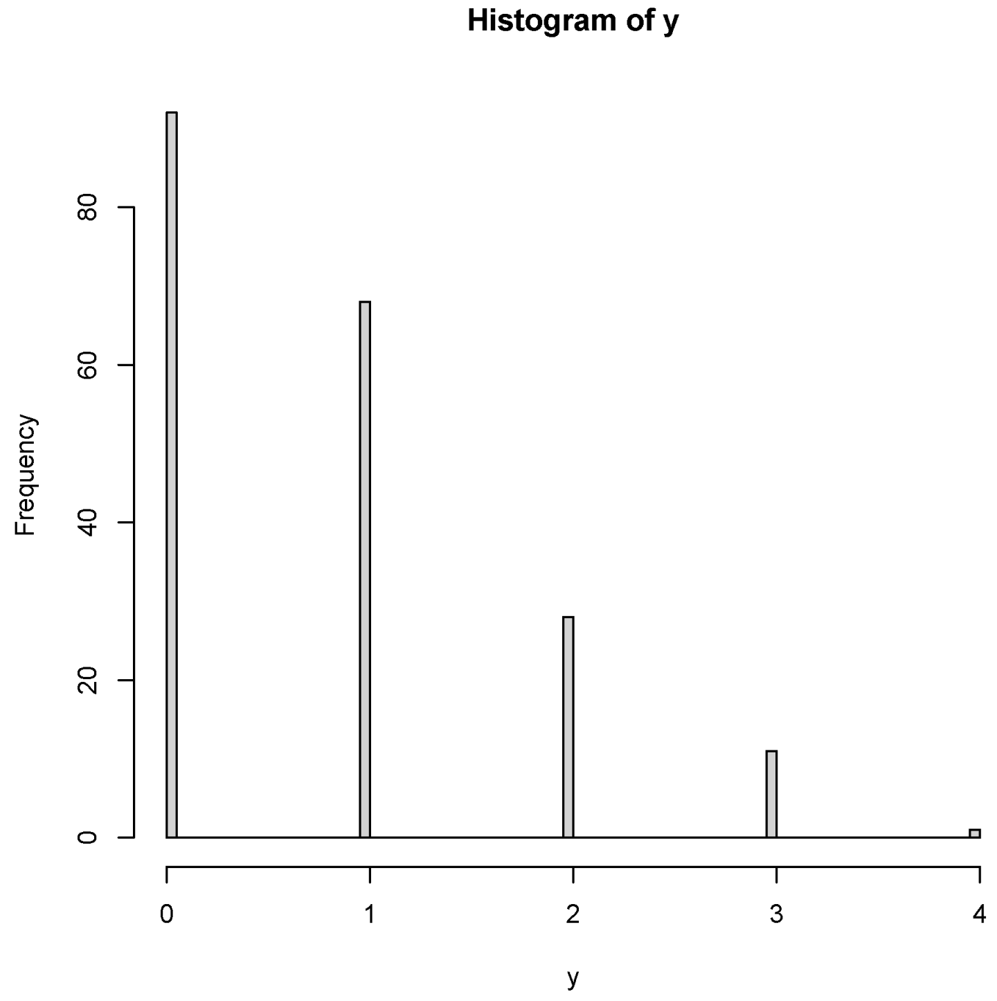
First, let us assume a mean parameter λ = 2 for a Poisson distribution. After this, we simulate n = 10,000 values from the Poisson distribution with the mean parameter λ = 2 , and the data obtained is denoted by y . The histogram of y is plotted in Figure 3. From this figure, we observe that the most frequent values are 1 and 2.
Second, let us plot the POM (Population Origin Moment, that is, E Y k by (9)), POM_hat (the estimated POM, that is, E Y k in (9) with λ estimated by the sample mean λ ^ = y ¯ ), and SOM (Sample Origin Moment, that is, A k = 1 n i = 1 n y i k ) for k = 1 , 2 , , 10 in Figure 4. From the figure, we see that POM and POM_hat are very close, while the SOM differs from the POM for large k values.
Third, the numerical values presented in Figure 4 are summarized in Table 2. In this table, the relative errors of POM_hat and SOM are defined as
re _ POM _ hat = POM POM _ hat POM , re _ SOM = POM SOM POM .
From the table, we observe that the relative error of POM_hat increases very slowly for all k, and they are very small, with the largest one being 1.7 % . However, the relative error of the SOM increases very fast, and it is as high as 27.7 % for the 10th origin moment.

8. Two Empirical Data Examples

We aim to present two empirical data examples to demonstrate the computation of higher-order POM approximations for the Poisson distribution in this section.
Example 1
(Telephone calls; Example 5.11 in [24]). In this example, the frequency of calls received by a telephone switchboard during a certain period of time is reported in Table 3. The data y is
0 0 0 0 0 0 0 1 1 1 1 1 1 1 1 1 1 2 2 2 2 2 2 2 2 2 2 2 2 3 3 3 3 3 3 3 3 4 4 4 5 5 ,
and the sample size of the data is 42. The sample mean of the data is y ¯ = 1.904762 .
A histogram of the telephone call data y is plotted in Figure 5. From Table 3 and Figure 5, we see that the most frequent number of calls received by the telephone switchboard during a certain period of time is 2, which is near the sample mean of 1.904762 .
Now let us conduct a chi-squared test for the data y to see whether this data can be considered to come from a Poisson distribution. The hypotheses are
H0 
The data are drawn from a Poisson distribution.
H1 
The data do not follow a Poisson distribution.
The chi-squared test gives a p-value of 0.9591 > 0.05 = α , indicating that the data y can be considered to come from a Poisson distribution. The mean parameter of the Poisson distribution is estimated as
λ ^ = y ¯ = 1.904762 .
POM_hat, the SOM, the difference between POM_hat and the SOM, and the relative error of POM_hat and the SOM for the telephone call data are presented in Table 4. From this table, we observe that the difference between POM_hat and the SOM increases very fast as k increases. Moreover, the relative error of POM_hat and the SOM also increases very fast as k increases, and it is as high as 83.5 % for k = 10 .
Example 2
(Number of customers, Exercise 5.9 in [24]). In this example, the number of customers entering a store per minute is reported in Table 5. The size of the data y is 200, and the sample mean of the data is y ¯ = 0.805 .
A histogram depicting the distribution of the customer data y is presented in Figure 6. From Table 5 and Figure 6, we observe that the most frequent number of customers entering a store per minute is 0, which is near the sample mean of 0.805 .
The chi-squared test gives a p-value of 0.8267 > 0.05 = α , indicating that the data y can be considered to come from a Poisson distribution. The mean parameter of the Poisson distribution is estimated as
λ ^ = y ¯ = 0.805 .
POM_hat, the SOM, the difference between POM_hat and the SOM, and the relative error of POM_hat and the SOM for the data on the number of customers are summarized in Table 6. From this table, we observe that the difference between POM_hat and the SOM increases very fast as k increases. Moreover, the relative error of POM_hat and the SOM also increases very fast as k increases, and it is as high as 79.2 % for k = 10 .

9. Conclusions and Discussions

This paper makes distinct theoretical contributions by bridging the theory of Poisson moments with combinatorial identities via the expectation identity method. Although it is known that the higher-order origin moments of the Poisson distribution are Touchard polynomials, this work independently derives them through a probabilistic technique—offering a clear and self-contained pathway that avoids infinite series. More significantly, we discover and rigorously prove two previously undocumented recurrence relations for Stirling numbers of the second kind: an L recurrence and a vertical recurrence. These relations not only deliver a recursive framework for efficiently computing the coefficients of these moments but also enrich the combinatorial literature. Thus, this study provides both a practical tool for moment computation and novel insights into the structure of Stirling numbers.
Numerical simulations and empirical applications substantiate the utility of our theoretical results. Simulations reveal that SOMs become increasingly biased for higher orders, with relative errors exceeding 27 % for the 10th moment. In contrast, the estimates derived from our method (POM_hat) remain accurate, with errors below 2 % . Analyses of real datasets—of telephone call counts and customer arrivals—confirm the Poisson model’s validity via chi-square tests. More importantly, they demonstrate that the SOMs diverge rapidly from the true moment values as the order increases, whereas POM_hat maintains consistency, underscoring the necessity of analytical moment expressions for reliable high-order inference.
Our method for computing higher-order Poisson moments has significant practical utility in fields requiring precise quantification of tail behavior or extreme events. This includes actuarial science for modeling claim counts, telecommunications for queuing system analysis, and risk management for assessing the probability of rare, high-impact occurrences. The analytical expressions we provide offer more reliable estimates than unstable sample moments, enabling better-informed decisions in these applied domains.
A standard formula for moments of any order for the Poisson distribution is fully documented. For example, see the summary at https://en.wikipedia.org/wiki/Poisson_distribution, accessed on 27 September 2025. In that discussion, under the heading “Higher Moments”, we find the well-known formula for moments (about zero) expressed in terms of Stirling numbers of the second kind. This result has been known since at least 1937. See [25,26]. Our goal was not to rediscover this known relationships but to provide a novel probabilistic derivation via expectation identities and, crucially, to prove the new L-shaped and vertical recurrence relations that the Stirling numbers themselves satisfy, which are novel contributions.

Author Contributions

Conceptualization: Y.-Y.Z.; formal analysis: Y.-Y.Z.; funding acquisition: Y.-Y.Z.; methodology: Y.-Y.Z. and D.-D.P.; software: Y.-Y.Z.; validation: Y.-Y.Z.; writing—original draft: Y.-Y.Z.; writing—review and editing: Y.-Y.Z. and D.-D.P. All authors have read and agreed to the published version of the manuscript.

Funding

The National Social Science Fund of China (21XTJ001) supported this research.

Data Availability Statement

The data that support the findings of this study are described in the article.

Conflicts of Interest

The authors declare no conflicts of interest.

Appendix A

In the appendix, we provide some proofs of the theorems.
Proof of Theorem 2.
We shall employ the principle of mathematical induction to rigorously demonstrate Theorem 2.
(1) When k equals 1,
E Y 1 = j = 0 1 a 1 , j λ j = a 1 , 0 λ 0 + a 1 , 1 λ 1 = λ ,
and thus, (3) is correct when k = 1 ;
(2) Suppose that (3) is correct when 1 k m ;
(3) This holds when k equals m + 1 .
Step 1: Apply the expectation identity. For g ( y ) = y m , Theorem 1 yields
E [ λ Y m ] = E [ Y ( Y 1 ) m ] .
The right-hand side is expanded using the binomial theorem and then simplified into a sum of lower-order moments, E Y l , which allows the desired term E Y m + 1 to be isolated on one side of the equation.
From (2), we have
E λ Y m = E Y Y 1 m = E Y i = 0 m m i Y i 1 m i = E i = 0 m 1 m i m i Y i + 1 = i = 0 m 1 m i m i E Y i + 1 = l = 1 m + 1 1 m l + 1 m l 1 E Y l ( l = i + 1 ) = l = 1 m 1 m l + 1 m l 1 E Y l + 1 0 m m E Y m + 1 = l = 1 m 1 m l + 1 m l 1 E Y l + E Y m + 1 .
Therefore,
E Y m + 1 = λ E Y m l = 1 m 1 m l + 1 m l 1 E Y l = λ E Y m + l = 1 m 1 m l m l 1 E Y l .
Step 2: Substitute the inductive hypothesis. The assumed moment formula (3) for all orders l m is substituted into Equation (A1). This expresses E Y m + 1 entirely in terms of the coefficients a ( l , j ) and powers of λ .
Since (3) is correct when 1 k m , we have
E Y m = j = 1 m a m , j λ j ,
E Y l = j = 1 l a l , j λ j ,
for 1 l m . Substituting (A2) and (A3) into (A1), we obtain
E Y m + 1 = λ j = 1 m a m , j λ j + l = 1 m 1 m l m l 1 j = 1 l a l , j λ j .
Step 3: Re-index and match the coefficients. The resulting expression is a polynomial in λ . By meticulously changing the summation indices and grouping terms with the same power of λ , the formula is rearranged into the form j a ( m + 1 , j ) λ j . Comparing the coefficients for each λ j confirms that the coefficients a ( m + 1 , j ) satisfy the proposed recurrence relation (5), thus completing the inductive step.
Let
S 1 = l = 1 m 1 m l m l 1 j = 1 l a l , j λ j = l = 1 m j = 1 l 1 m l m l 1 a l , j λ j .
After the change in the order of summations, we obtain
l = 1 m j = 1 l f l j = j = 1 m l = j m f l j .
Let
f l j = 1 m l m l 1 a l , j λ j .
According to (A6), (A5) reduces to
S 1 = l = 1 m j = 1 l f l j = j = 1 m l = j m f l j = j = 1 m l = j m 1 m l m l 1 a l , j λ j = j = 1 m l = j m 1 m l m l 1 a l , j λ j .
Substituting (A7) into (A4), we have
E Y m + 1 = j = 1 m a m , j λ j + 1 + j = 1 m l = j m 1 m l m l 1 a l , j λ j .
Let j + 1 = n . Then,
j = 1 m a m , j λ j + 1 = n = 2 m + 1 a m , n 1 λ n = n = 2 m a m , n 1 λ n + a m , m λ m + 1 .
After that, changing the summation index n back to j in the above summation, we obtain
j = 1 m a m , j λ j + 1 = j = 2 m a m , j 1 λ j + a m , m λ m + 1 .
Substituting (A9) into (A8) and rearranging, we obtain
E Y m + 1 = j = 2 m a m , j 1 λ j + a m , m λ m + 1 + j = 1 m l = j m 1 m l m l 1 a l , j λ j = j = 2 m a m , j 1 λ j + a m , m λ m + 1 + j = 2 m l = j m 1 m l m l 1 a l , j λ j + l = 1 m 1 m l m l 1 a l , 1 λ = l = 1 m 1 m l m l 1 a l , 1 λ + j = 2 m a m , j 1 + l = j m 1 m l m l 1 a l , j λ j + a m , m λ m + 1 = j = 1 m + 1 a m + 1 , j λ j .
In (A10), it can be verified that
a m + 1 , 1 = l = 1 m 1 m l m l 1 a l , 1 = 1 .
Moreover, for j = 2 , , m ,
a m + 1 , j = a m , j 1 + l = j m 1 m l m l 1 a l , j = a m , j 1 + l = j m 1 m + 1 l + 1 m l 1 a l , j ,
which is in the form of (5) with k = m + 1 . In addition,
a m + 1 , m + 1 = a m , m = 1 .
Therefore, when k = m + 1 , (3) also holds true.
To summarize, through the application of mathematical induction, we have established (3), thereby completing the proof of the theorem. □
Proof of Theorem 3.
We provide two methods to prove (7).
Method 1. Utilizing the exponential generating function for S ( n , j ) .
Proof strategy: We use the standard recurrence for Stirling numbers of the second kind:
S ( k , j ) = S ( k 1 , j 1 ) + j S ( k 1 , j ) .
We will show that the summation in (7) equals j S ( k 1 , j ) . Substituting this into the standard recurrence yields the given formula. The boundary conditions follow directly from the definition.
Detailed proof is given as follows.
Step 1: Prove the summation equals j S ( k 1 , j ) . Consider the summation
m = j k 1 ( 1 ) k m + 1 k 1 m 1 S ( m , j ) .
Substitute n = k 1 , so the sum becomes
m = j n ( 1 ) ( n + 1 ) m + 1 n m 1 S ( m , j ) = m = j n ( 1 ) n m + 2 n m 1 S ( m , j ) = m = j n ( 1 ) n m n m 1 S ( m , j ) .
Define the sequence
b n = m = j n ( 1 ) n m + 1 n m 1 S ( m , j ) .
The original sum is b n (sign-reversed). We will prove b n = j S ( n , j ) , so
m = j n ( 1 ) n m n m 1 S ( m , j ) = b n = ( j S ( n , j ) ) = j S ( n , j ) .
Since n = k 1 , this gives
m = j k 1 ( 1 ) k m + 1 k 1 m 1 S ( m , j ) = j S ( k 1 , j ) .
To prove b n = j S ( n , j ) , use exponential generating functions. The exponential generating function for S ( n , j ) is
n = j S ( n , j ) x n n ! = ( e x 1 ) j j ! .
Define the exponential generating function for b n ,
B j ( x ) = n = j b n x n n ! .
Substitute the definition of b n ,
b n = m = j n ( 1 ) n m + 1 n m 1 S ( m , j ) ,
so
b n n ! = m = j n ( 1 ) n m + 1 S ( m , j ) ( m 1 ) ! ( n m + 1 ) ! .
Thus,
B j ( x ) = n = j m = j n ( 1 ) n m + 1 S ( m , j ) ( m 1 ) ! ( n m + 1 ) ! x n .
Swap the sums (fix m, sum over n m ),
B j ( x ) = m = j S ( m , j ) ( m 1 ) ! ( 1 ) n = m ( 1 ) n m x n ( n m + 1 ) ! .
For the inner sum, let k = n m + 1 (so n = m + k 1 , and k = 1 when n = m ),
n = m ( 1 ) n m x n ( n m + 1 ) ! = k = 1 ( 1 ) k 1 x m + k 1 k ! .
Since ( 1 ) k 1 = ( 1 ) k ,
k = 1 ( 1 ) k 1 x m + k 1 k ! = x m 1 k = 1 ( x ) k k ! = x m 1 ( e x 1 ) .
Substitute back:
B j ( x ) = m = j S ( m , j ) ( m 1 ) ! ( 1 ) x m 1 ( e x 1 ) = m = j S ( m , j ) x m 1 ( m 1 ) ! ( e x 1 ) .
Let v = m 1 :
m = j S ( m , j ) x m 1 ( m 1 ) ! = v = j 1 S ( v + 1 , j ) x v v ! .
The exponential generating function for S ( v + 1 , j ) is the derivative of the original:
v = j 1 S ( v + 1 , j ) x v v ! = d d x ( e x 1 ) j j ! = j ( e x 1 ) j 1 e x j ! = ( e x 1 ) j 1 e x ( j 1 ) ! .
Hence,
B j ( x ) = ( e x 1 ) j 1 e x ( j 1 ) ! ( e x 1 ) = ( e x 1 ) j 1 ( j 1 ) ! ( 1 e x ) = ( e x 1 ) j 1 ( j 1 ) ! ( ( e x 1 ) ) = ( e x 1 ) j ( j 1 ) ! .
Rewrite
( e x 1 ) j ( j 1 ) ! = j · ( e x 1 ) j j ! = j n = j S ( n , j ) x n n ! .
So,
B j ( x ) = j n = j S ( n , j ) x n n ! = n = j b n x n n ! .
Comparing coefficients,
b n = j S ( n , j ) .
Therefore,
m = j n ( 1 ) n m n m 1 S ( m , j ) = j S ( n , j ) .
With n = k 1 ,
m = j k 1 ( 1 ) k m + 1 k 1 m 1 S ( m , j ) = j S ( k 1 , j ) .
Step 2: Substitute into the standard recurrence. The standard recurrence is
S ( k , j ) = S ( k 1 , j 1 ) + j S ( k 1 , j ) .
Replacing j S ( k 1 , j ) with the summation,
S ( k , j ) = S ( k 1 , j 1 ) + m = j k 1 ( 1 ) k m + 1 k 1 m 1 S ( m , j ) .
This matches the recurrence in (7).
Step 3: Verify the boundary conditions and range.
Boundary conditions: For j = 1 or j = k , S ( k , 1 ) = 1 and S ( k , k ) = 1 by definition.
Case j = k : The sum is over m from k to k 1 , which is empty (sum = 0). Since S ( k 1 , k 1 ) = 1 , we have S ( k , k ) = 1 + 0 = 1 , consistent.
Case j = 1 : The recurrence is not applied (since j 2 in the theorem), but the boundary condition holds.
Range j = 2 , , k 1 : The recurrence holds as shown.
Thus, the theorem is proven.
Method 2. Utilizing mathematical induction.
Through the triangular recurrence relation, we have
S k , j = S k 1 , j 1 + j S k 1 , j .
Substituting (A11) into (7), we obtain
S k 1 , j 1 + j S k 1 , j = S k 1 , j 1 + l = j k 1 1 k l + 1 k 1 l 1 S l , j
j S k 1 , j = l = j k 1 1 k l + 1 k 1 l 1 S l , j
j S k 1 , j = l = j k 2 1 k l + 1 k 1 l 1 S l , j + k 1 S k 1 , j
j k + 1 S k 1 , j = l = j k 2 1 k l + 1 k 1 l 1 S l , j .
Let n = k 1 , and then k = n + 1 and j = 2 , , n (since j k 1 = n ). Substituting n = k 1 into (A12), the equation changes to
j n S n , j = l = j n 1 1 n l n l 1 S l , j .
Now, let us utilize the mathematical induction method to prove (A13). Fix j 2 and induction for n j .
(1) When n = j ,
L H S = j j S j , j = 0 · 1 = 0 , R H S = l = j j 1 = 0 ( the sum is empty ) .
(A13) holds true.
(2) Assume that (A13) is correct for m < n .
(3) Let us prove that (A13) is correct for n.
L H S = j n S n , j , R H S = l = j n 1 1 n l n l 1 S l , j .
It is easy to show that
R H S = 1 n n 1 n n 1 1 S n 1 , j + l = j n 2 1 n l n l 1 S l , j = n 2 S n 1 , j + l = j n 2 1 n l n l 1 S l , j .
According to the Pascal identity for binomial coefficients, we have
n l 1 = n 1 l 1 + n 1 l 2 .
Therefore,
l = j n 2 1 n l n l 1 S l , j = l = j n 2 1 n l n 1 l 1 S l , j + l = j n 2 1 n l n 1 l 2 S l , j .
The first term is
l = j n 2 1 n l n 1 l 1 S l , j = l = j n 2 1 n 1 l n 1 l 1 S l , j .
Through mathematical induction (for n 1 and j),
l = j n 2 1 n 1 l n 1 l 1 S l , j = j n 1 S n 1 , j .
Hence, the first term reduces to
j n + 1 S n 1 , j .
For the second term,
l = j n 2 1 n l n 1 l 2 S l , j .
Let k = l 1 , and then l = k + 1 . The second term changes to
k = j 1 n 3 1 n k + 1 n 1 k 1 S k + 1 , j = k = j 1 n 3 1 n k 1 n 1 k 1 S k + 1 , j .
According to the triangular recurrence relation, we have
S k + 1 , j = j S k , j + S k , j 1 .
Therefore, the second term reduces to
k = j 1 n 3 1 n k 1 n 1 k 1 j S k , j + S k , j 1 = j k = j 1 n 3 1 n k 1 n 1 k 1 S k , j + k = j 1 n 3 1 n k 1 n 1 k 1 S k , j 1 j A + D ,
where
A = k = j 1 n 3 1 n 1 k n 1 k 1 S k , j , D = k = j 1 n 3 1 n 1 k n 1 k 1 S k , j 1 .
Through mathematical induction,
1 For n 1 and j,
l = j n 2 1 n 1 l n 1 l 1 S l , j = j n + 1 S n 1 , j ,
and S j 1 , j = 0 , we have
A = j n + 1 S n 1 , j + n 1 2 S n 2 , j .
2 For n 1 and j 1 ,
l = j 1 n 2 1 n 1 l n 1 l 1 S l , j 1 = j n S n 1 , j 1 ,
we obtain
D = j n S n 1 , j 1 + n 1 2 S n 2 , j 1 .
Consequently, the second term becomes
j A + D = j j n + 1 S n 1 , j + n 1 2 S n 2 , j + j n S n 1 , j 1 + n 1 2 S n 2 , j 1 .
Combining the parts of the R H S , we have
R H S = n 2 S n 1 , j j n + 1 S n 1 , j + j A + D = n 2 S n 1 , j j n + 1 S n 1 , j + j j n + 1 S n 1 , j + j n 1 2 S n 2 , j + j n S n 1 , j 1 + n 1 2 S n 2 , j 1 .
The L H S becomes
j n S n , j = j n j S n 1 , j + S n 1 , j 1 .
Computing R H S L H S , and utilizing the triangular recurrence relation
S n 1 , j = j S n 2 , j + S n 2 , j 1 ,
we find the difference is 0. That is, the two sides are equal. Therefore, (A13) is correct for n. Finally, (7) is proven. □

References

  1. Paloheimo, J.E. Spatial bivariate Poisson distribution. Biometrika 1972, 59, 489–492. [Google Scholar] [CrossRef]
  2. Steyn, H.S. Multivariate Poisson normal distribution. J. Am. Stat. Assoc. 1976, 71, 233–236. [Google Scholar] [CrossRef]
  3. Lukacs, E.; Beer, S. Characterization of multivariate Poisson-distribution. J. Multivar. Anal. 1977, 7, 1–12. [Google Scholar] [CrossRef]
  4. Aitchison, J.; Ho, C.H. The multivariate Poisson-log normal-distribution. Biometrika 1989, 76, 643–653. [Google Scholar] [CrossRef]
  5. Chen, L.H.Y. Convergence of Poisson binomial to Poisson distributions. Ann. Probab. 1974, 2, 178–180. [Google Scholar] [CrossRef]
  6. Duembgen, L.; Wellner, J.A. The density ratio of Poisson binomial versus Poisson distributions. Stat. Probab. Lett. 2020, 165, 108862. [Google Scholar] [CrossRef]
  7. Cordeiro, G.M.; Rodrigues, J.; de Castro, M. The exponential COM-Poisson distribution. Stat. Pap. 2012, 53, 653–664. [Google Scholar] [CrossRef]
  8. Atkinson, A.C.; Yeh, L. Inference for Sichel compound Poisson-distribution. J. Am. Stat. Assoc. 1982, 77, 153–158. [Google Scholar] [CrossRef]
  9. Roos, B. Improvements in the Poisson approximation of mixed Poisson distributions. J. Stat. Plan. Inference 2003, 113, 467–483. [Google Scholar] [CrossRef]
  10. Alzaid, A.A.; Alqefari, A.A.; Qarmalah, N. On the conflation of Poisson and logarithmic distributions with applications. Axioms 2025, 14, 518. [Google Scholar] [CrossRef]
  11. Wu, H.J.; Zhang, Y.Y.; Li, H.Y. Expectation identities from integration by parts for univariate continuous random variables with applications to high-order moments. Stat. Pap. 2023, 64, 477–496. [Google Scholar] [CrossRef]
  12. Zhang, Y.Y.; Rong, T.Z.; Li, M.M. Expectation identity for the binomial distribution and its application in the calculations of high-order binomial moments. Commun. Stat.-Theory Methods 2019, 48, 5467–5476. [Google Scholar] [CrossRef]
  13. Liu, J.L.; Zhang, Y.Y.; Wang, Y.Q. Expectation identity of the discrete uniform distribution and its application in the calculations of higher-order origin moments. Adv. Appl. Stat. 2023, 85, 1–41. [Google Scholar] [CrossRef]
  14. Wang, Y.Q.; Zhang, Y.Y.; Liu, J.L. Expectation identity of the hypergeometric distribution and its application in the calculations of high-order origin moments. Commun. Stat.-Theory Methods 2023, 52, 6018–6036. [Google Scholar] [CrossRef]
  15. Zhang, Y.Y. Expectation identity of the negative binomial distribution and its application in the calculations of high-order origin moments. Commun. Stat.-Theory Methods 2025, 54, 6701–6710. [Google Scholar] [CrossRef]
  16. Casella, G.; Berger, R.L. Statistical Inference, 2nd ed; Duxbury: Pacific Grove, CA, USA, 2002. [Google Scholar]
  17. Hwang, J.T. Improving on standard estimators in discrete exponential families with applications to Poisson and negative binomial cases. Ann. Stat. 1982, 10, 857–867. [Google Scholar] [CrossRef]
  18. R Core Team. R: A Language and Environment for Statistical Computing; R Foundation for Statistical Computing: Vienna, Austria, 2024. [Google Scholar]
  19. Comtet, L. Advanced Combinatorics, Revised and Enlarged ed.; D. Reidel Publishing Company: Boston, MA, USA, 1974. [Google Scholar]
  20. Simsek, B. New moment formulas for moments and characteristic function of the geometric distribution in terms of Apostol-Bernoulli polynomials and numbers. Math. Methods Appl. Sci. 2024, 47, 9169–9179. [Google Scholar] [CrossRef]
  21. Simsek, B. Novel formulas of moments of negative binomial distribution connected with Apostol-Bernoulli numbers of higher order and Stirling numbers. Rev. Real Acad. Cienc. Exactas Fis. Nat. Ser. A Mat. 2024, 118, 142. [Google Scholar] [CrossRef]
  22. Simsek, B. Certain mathematical formulas for moments of geometric distribution by means of the Apostol-Bernoulli polynomials. Filomat 2025, 39, 1843–1853. [Google Scholar] [CrossRef]
  23. Simsek, B.; Kilar, N. By analysis of moments of geometric distribution: New formulas involving Eulerian and Fubini numbers. Appl. Anal. Discret. Math. 2025, 19, 233–252. [Google Scholar] [CrossRef]
  24. Xue, Y.; Chen, L.P. Statistical Modeling and R Software; Tsinghua University Press: Beijing, China, 2007. [Google Scholar]
  25. Riordan, J. Moment recurrence relations for binomial, Poisson and hypergeometric frequency distributions. Ann. Math. Stat. 1937, 8, 103–111. [Google Scholar] [CrossRef]
  26. Haight, F.A. Handbook of the Poisson Distribution; John Wiley & Sons: New York, NY, USA, 1967. [Google Scholar]
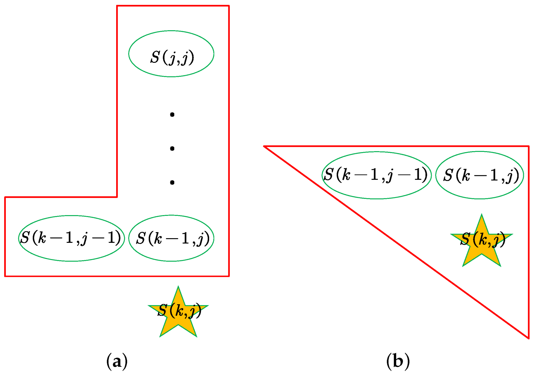
Figure 1. Schematic plots of the recurrence relations of (7). (a) L recurrence relation ( k 1 > j ); (b) triangular recurrence relation ( k 1 = j ).
Axioms 14 00747 g001
Figure 2. A schematic plot of the vertical recurrence relation of (8).
Axioms 14 00747 g002
Figure 3. The histogram of y .
Axioms 14 00747 g003
Figure 4. The POM, POM_hat, and SOM for k = 1 , 2 , , 10 .
Axioms 14 00747 g004
Figure 5. A histogram of the telephone call data y .
Axioms 14 00747 g005
Figure 6. A histogram of the data on the number of customers y .
Axioms 14 00747 g006
Table 1. The coefficients associated with the first 10 origin moments of the Poisson distribution.
j = 0 12345678910
k = 0 1
101
2011
30131
401761
5011525101
601319065151
70163301350140211
80112796617011050266281
9012553025777069512646462361
1001511933034,10542,52522,8275880750451
Table 2. POM, POM_hat, SOM, the differences from POM, and the relative errors for k = 1 , 2 , , 10 .
k12345678910
POM 2.000 6.000 22.094.0454.02430.014,214.089,918.0610,182.04,412,798.0
POM _ hat 2.006 6.03022.194.8458.62458.214,399.591,216.8619,823.54,488,357.1
POM POM _ hat 0.006 0.030 0.1 0.8 4.6 28.2 185.5 1298.8 9641.5 −75,559.1
re _ POM _ hat 0.3 % 0.5 % 0.7 % 0.9 % 1.0 % 1.2 % 1.3 % 1.4 % 1.6 % 1.7 %
SOM 2.006 6.065 22.394.5446.52306.812,844.876,342.3480,766.03,188,704.9
POM SOM 0.006 0.065 0.3 0.5 7.5 123.21369.213,575.7129,416.01,224,093.1
re _ SOM 0.3 % 1.1 % 1.3 % 0.5 % 1.6 % 5.1 % 9.6 % 15.1 % 21.2 % 27.7 %
Table 3. The frequency of calls received by the telephone switchboard during a certain period of time.
Number of calls received0123456
Frequency of occurrence710128320
Table 4. POM_hat, the SOM, the difference between POM_hat and the SOM, and the relative error of POM_hat and the SOM for the telephone call data for k = 1 , 2 , , 10 .
k12345678910
POM _ hat 1.905 5.519.781.9385.82015.811,521.871,279.5473,353.4 3 , 351 , 975.2
SOM 1.905 5.4 18.268.3277.61194.05343.924,605.4115,626.2551,468.3
POM _ hat SOM 0.000 0.11.513.6108.2821.86177.946,674.1357,727.22,800,506.9
re 0.0 % 1.9 % 7.7 % 16.7 % 28.0 % 40.8 % 53.6 % 65.5 % 75.6 % 83.5 %
Table 5. The number of customers entering a store per minute.
Number of customers012345
Frequency of occurrence9268281110
Table 6. POM_hat, the SOM, the difference between POM_hat and the SOM, and the relative error of POM_hat and the SOM for the data on the number of customers for k = 1 , 2 , , 10 .
k12345678910
POM _ hat 0.805 1.4533.2718.928.1100.5398.91735.08184.541,535.2
SOM 0.805 1.475 3.2658.323.369.9220.5724.72465.38634.3
POM _ hat SOM 0.000 0.022 0.0060.64.830.6178.41010.35719.232,901.0
re 0.0 % 1.5 % 0.2%6.5%17.1%30.5%44.7%58.2%69.9%79.2%
Disclaimer/Publisher’s Note: The statements, opinions and data contained in all publications are solely those of the individual author(s) and contributor(s) and not of MDPI and/or the editor(s). MDPI and/or the editor(s) disclaim responsibility for any injury to people or property resulting from any ideas, methods, instructions or products referred to in the content.