Article

Fusion Maximal Information Coefficient-Based Quality-Related Kernel Component Analysis: Mathematical Formulation and an Application for Nonlinear Fault Detection

by
Jie Yuan
1,
Hao Ma
2,* and
Yan Wang
2,*
1
School of Automation, Wuxi University, Wuxi 214122, China
2
School of Internet of Things Engineering, Jiangnan University, Wuxi 214122, China
*
Authors to whom correspondence should be addressed.
Axioms 2025, 14(10), 745; https://doi.org/10.3390/axioms14100745
Submission received: 21 August 2025 / Revised: 23 September 2025 / Accepted: 28 September 2025 / Published: 30 September 2025

Abstract

Amid intensifying global competition, industrial product quality has become a critical determinant of competitive advantage. However, persistent quality-related faults in production environments threaten product integrity. To address this challenge, a Fusion Maximal Information Coefficient-based Quality-Related Kernel Component Analysis (FMIC-QRKCA) methodology is proposed in this paper by capitalizing on information fusion principles and statistical metric theory. Based on information fusion principles, a Fusion Maximal Information Coefficient (FMIC) strategy is first studied to quantify correlations between process variables and multivariate quality indicators. Subsequently, by integrating the proposed FMIC method with Kernel Principal Component Analysis (KPCA), a Quality-Related Kernel Component Analysis (QRKCA) method is proposed. In the proposed QRKCA strategy, the complete latent variable space is first obtained; on this basis, FMIC is further applied to quantify the correlation between each latent variable and quality variables, thereby completing the screening of quality-related latent variables. Additionally, the T 2 and squared prediction error monitoring statistics are used as the key indices to determine the occurrence of faults. This integration overcomes the limitation of conventional KPCA, which does not explicitly consider quality indicators during the principal component extraction, thereby enabling precise isolation of quality-related fault features. Validation through the numerical case and the industrial process case demonstrates that FMIC-QRKCA significantly outperforms established methods in detection accuracy for quality-related faults.

1. Introduction

In modern engineering and industrial systems, fault detection serves as a core link for ensuring equipment reliability, operational safety, and economic efficiency, whose technical essence can be attributed to the problem of statistical correlation analysis, feature selection, and optimization modeling for high-dimensional nonlinear data. By identifying system anomalies and potential faults at an early stage, fault detection enables timely maintenance interventions, thereby effectively preventing catastrophic shutdowns, reducing unplanned equipment downtime, and minimizing economic losses [1,2].
From the perspective of technical pathways, fault detection methods are mainly categorized into two types: model-based and data-driven approaches [3]. Among them, the core logic of model-based methods lies in constructing accurate mathematical models that describe the normal operating state of the system. Faults are determined by monitoring deviations between the actual system behavior and the predicted values of the model. For example, for linear time-invariant (LTI) systems (a common baseline for industrial dynamic systems), the normal state is typically described using a state-space model, which can be expressed as
x ( k + 1 ) = A x ( k ) + B u ( k ) + w ( k ) , y ( k ) = C x ( k ) + D u ( k ) + v ( k ) ,
where x ( k ) represents the system state at k, u ( k ) and y ( k ) represent the input and output of the system, respectively, A , B , C , and D are the system matrices, which can be identified via system identification methods, w ( k ) and v ( k ) denote the process and measurement noise. In this case, faults can be detected by monitoring the residuals, which are the deviations between actual and model-predicted outputs,
r ( k ) = y ( k ) y ^ ( k ) ,
where y ( k ) is the model predicted output. A fault is declared if the residual exceeds a predefined threshold δ . However, in complex industrial scenarios, this type of method faces significant bottlenecks, which are due to difficulties in accurately modeling nonlinear systems, environmental uncertainties, and time-varying characteristics, its applicability and detection accuracy often fail to meet practical requirements [4,5].
In contrast, data-driven methods take massive historical and real-time operational data as their core input. Without relying on explicit mathematical models of the system, they automatically learn characteristic patterns of normal and fault states through algorithms. For a typical data-driven workflow, let X = [ x 1 , x 2 , x 3 , , x n ] denote the process matrix, and Y = [ y 1 , y 2 , y 3 , , y n ] denotes the output matrix. On the basis of this, the data-driven modeling methods can be used to model the relationship between the process and output matrices, which can be expressed as
Y = f d a t a d r i v e n ( X , Θ ) ,
where Θ denotes the unknown parameters of the data-driven function f d a t a d r i v e n ( · ) . Then, the established model is used to obtain the predicted output of online data, and the residual of the output is similarly calculated to detect the occurrence of faults. This data-driven modeling characteristic allows them to exhibit unique advantages in complex dynamic systems where traditional model-based methods are difficult to adapt, making them one of the mainstream research directions in the field of industrial fault detection currently [6].
Within the domain of data-driven fault detection, Multivariate Statistical Analysis (MSA) represents a fundamental methodology [7,8]. MSA techniques excel at processing complex, high-dimensional datasets prevalent in modern industrial systems. A primary advantage is their capability to model complex interdependencies and correlations among process variables, providing a holistic representation of system behavior. These methods effectively extract latent patterns and features, facilitating the detection of faults. The fundamental MSA methods include Principal Component Analysis (PCA), Canonical Correlation Analysis (CCA), and Partial Least Squares (PLS) [9,10,11]. PCA performs unsupervised dimensionality reduction by identifying principal components that maximize variance in the process variable space [12]. CCA explores relationships between two sets of variables by finding canonical variates that maximize cross-correlation, revealing shared covariance structures [13]. In contrast, PLS is a supervised regression technique that simultaneously projects both predictors and responses into latent spaces to maximize covariance between them, making it particularly effective for predictive modeling with multicollinear or high-dimensional data [14].
Quality-related fault detection fundamentally differs from traditional fault detection approaches. Whereas traditional methods primarily distinguish between faulty and non-faulty states, quality-related fault detection further classifies system states into three conditions based on their impact on quality indicators: quality-related faults, quality-unrelated faults, and fault-free operation. It is worth noting that the quality-related faults indicate a serious adverse impact on quality variables [15]. Within industrial processes, this methodology enables real-time process monitoring and control, allowing manufacturers to implement timely adjustments that ensure process stability and consistency. Consequently, it elevates product quality while optimizing production efficiency through reduced rework and scrap rates. Furthermore, it identifies latent production inefficiencies, providing actionable insights for process refinement and innovation that foster long-term sustainable development in industrial enterprises [16].
Given the distinct characteristics and significant value of quality-related fault detection, numerous MSA-based methods have been developed [17]. Jiao et al. proposed an orthogonal kernel principal component regression method to address quality-related root cause diagnosis in nonlinear processes [18]. Wang et al. integrated the kernel PCA (KPCA) and CCA methods and proposed a KPCA-CCA for quality-related fault detection and diagnosis in nonlinear process monitoring, which extracts kernel principal components via KPCA and optimizes CCA using Singular Value Decomposition (SVD) technology [19]. Sun et al. developed a distributed kernel principal component regression method for plant-wide quality-related process monitoring [20]. Leveraging artificial neural networks, Chen et al. proposed an artificial neural correlation analysis to enhance the performance of the CCA method in quality-related fault detection [21].
Unlike the aforementioned PCA-based and CCA-based approaches, PLS-based methods, which integrate the advantages of PCA and CCA, have seen broader adoption in quality-related fault detection. However, studies reveal that standard PLS performs oblique decomposition of the process variable space, failing to decompose it into mutually orthogonal subspaces relative to the quality variable space. This limitation restricts its effectiveness in quality-related fault detection. To resolve this, Total PLS (T-PLS) and Total Kernel PLS (T-KPLS) methods were proposed to fully decompose the process variable space into four distinct subspaces [22,23]. Based on the idea of the aforementioned deep decomposition, the methods of Total Principal Component Regression (T-PCR) and Total Kernel Principal Component Regression (T-KPCR) have been proposed to achieve the orthonormal decomposition of the kernel space composed of process variables [24]. Additionally, a Modified KPLS (MKPLS) method utilizing SVD technology was developed to achieve orthogonal decomposition of the process variable space aligned with the quality variable space [25].
Although improved MSA-based strategies effectively address original limitations in quality-related fault detection, they fail to sufficiently prioritize quality-related faults [26,27]. In industrial practice, anomalies interfering with quality detection are inevitable. Persistent operator attention to such irrelevant anomalies undermines confidence in detection systems. Critically, as established by quality-related fault detection principles, operators prioritize faults impacting product quality. Thus, a key research gap remains: how to suppress detection of disturbances, noise, and quality-irrelevant anomalies while enhancing sensitivity to quality-related faults.
Motivated by the preceding analysis, this paper proposes a novel multivariate statistical methodology termed the Fusion Maximal Information Coefficient-based Quality-Related Kernel Component Analysis (FMIC-QRKCA). In the proposed strategy, the Fusion Maximal Information Coefficient (FMIC) method first leverages information fusion principles to quantify the correlations between individual process variables and multiple quality indicators, enabling quality-informed screening of process variables. The information fusion mentioned here specifically refers to integrating the correlations between the same process variable and different quality indicators into a comprehensive indicator based on the idea of Bayesian fusion [28]. Building upon FMIC and KPCA, the Quality-Related Kernel Component Analysis (QRKCA) method is studied to address a critical limitation of conventional KPCA, which neglects quality variables during principal component selection. The QRKCA methodology operates through three sequential steps: it first derives the complete principal component subspace from the kernel matrix of the process variable space; subsequently employs FMIC to quantify correlations between each principal component vector and multiple quality indicators; and finally applies a cumulative quality-relevant information percentage criterion to select quality-related principal components. Collectively, these innovations form an integrated framework for precise quality-related feature extraction in nonlinear industrial processes. The main contributions of this paper are summarized as follows.
(1)
A novel multivariate statistical methodology termed the FMIC-QRKCA method for quality-related fault detection in nonlinear industrial processes, explicitly addressing quality-related feature extraction to significantly enhance detection performance for quality-related faults.
(2)
Based on the information fusion and the MIC, a FMIC method is proposed to rigorously quantify the correlations between process variables and multivariate quality indicators, enabling targeted screening of quality-informative process variables through information fusion.
(3)
Building upon the fundamentals of FMIC and KPCA, a QRKCA method is developed, which advances traditional KPCA by incorporating quality relevance into principal component selection via statistical correlation analysis and cumulative information criteria.
The remainder of this paper is structured as follows: Section 2 introduces essential preliminaries and identifies limitations of conventional KPCA in quality-related fault detection. Section 3 details the proposed FMIC-QRKCA methodology and presents the complete quality-related monitoring framework. Section 4 validates the approach through two case studies with a comprehensive analysis. Finally, Section 5 concludes this paper.

2. Preliminaries

2.1. Methodological Review

For a nonlinear industrial process that contains m x process variables and m y quality variables, which are collected as x i R m x and y i R m y , respectively. Consider n offline training samples under normal conditions, and form the process variable matrix and the quality variable matrix as X R n × m x and Y R n × m y , which can be expressed as
X = [ x 1 , x 2 , x 3 , , x n ] T , Y = [ y 1 , y 2 , y 3 , , y n ] T .
To effectively characterize the nonlinear features inherent in the original process variable space, a commonly used and effective strategy is to map the process variable matrix X into a high-dimensional space Ψ ( X ) R n × . This transformation not only enhances the capability to identify complex patterns but also offers a more comprehensive understanding of the intricate structural relationships within the data.
Since the dimension of the process mapping matrix Ψ ( X ) is typically arbitrarily large or even infinite, the constructed mapping matrix Ψ ( X ) is unknown and unable to substitute for calculation. To address this issue, a kernel matrix K , composed of the inner product of the mapping matrix Ψ ( X ) , is typically introduced to facilitate the specific calculation, which can be represented as
K = Ψ ( X ) Ψ T ( X ) = k 1 , 1 k 1 , 2 k 1 , 3 k 1 , n k 2 , 1 k 2 , 2 k 2 , 3 k 2 , n k n , 1 k n , 2 k n , 3 k n , n R n × n ,
where k i , j = < ψ ( x i ) , ψ ( x j ) > = f ( x i , x j ) R ; f ( · ) denotes the kernel function. The Gaussian kernel function f ( · ) is typically employed to address this issue, which can be expressed as
f ( x i , x j ) = exp 1 c x i x j 2 ,
where c is the unknown kernel parameter. After nonlinear mapping, a crucial preliminary step before proceeding further is to preprocess the resultant process mapping space to ensure its mean is zero. Let Ψ ¯ ( X ) R n × denote the preprocessed Ψ ( X ) , which can be calculated as
Ψ ¯ ( X ) = I n 1 n 1 n 1 n T Ψ ( X ) .
Based on the obtained Ψ ¯ ( X ) , the kernel matrix with zero mean, denoted as K ¯ R n × n , can be calculated as
K ¯ = Ψ ¯ ( X ) Ψ ¯ T ( X ) = I n 1 n 1 n 1 n T Ψ ( X ) Ψ T ( X ) I n 1 n 1 n 1 n T = I n 1 n 1 n 1 n T K I n 1 n 1 n 1 n T .
Based on the aforementioned, the KPCA method achieves the decompositions of the kernel matrix K ¯ and the quality variable space Y . The main computational steps are outlined below.
Step 1. Perform eigenvalue decomposition on the obtained K ¯ ,
K ¯ U = U Λ ,
where U is the eigenvector matrix, and Λ denotes the diagonal matrix of eigenvalues.
Step 2. Sort the obtained eigenvalues in Λ in descending order. Correspondingly, reorder the eigenvectors in U to align with the sorted eigenvalues, resulting in a sorted eigenvector matrix U s o r t e d = [ u 1 , u 2 , , u n ] now corresponds to the i-th largest eigenvalue. Select the first k eigenvectors from U s o r t e d that correspond to the top k largest eigenvalues.
Step 3. Construct the projection matrix U k based on the selected feature vectors, and project the kernel matrix K ¯ onto the principal component molecular space T k ,
T k = K ¯ U k .
Here, each column of T k represents a principal component, capturing the dominant variance and correlation patterns in the original kernel matrix K ¯ .

2.2. Problem Description

In the KPCA method described above, high-dimensional mapping effectively captures the nonlinear characteristics of the data. Leveraging this mapping, the kernel matrix is decomposed to yield a principal component space and a residual space. However, the KPCA method exhibits the following limitations:
Problem 1. Both KPCA and traditional multivariate statistical methods perform analysis directly in the original process variable space. While this comprehensively captures hidden correlations among process variables, such an approach inevitably incorporates substantial redundant information during quality-related fault detection. This unnecessary complexity complicates subsequent operations.
Problem 2. Traditional KPCA, as an unsupervised learning technique, selects principal components exclusively by maximizing data variance. This approach prioritizes high-variance components while discarding low-variance ones. Although effective for capturing dominant variation patterns, it entirely disregards potential correlations between principal components and critical quality variables. Consequently, since quality-related faults manifest in features linked to these quality variables, KPCA fails to take quality factors into account, which hinders its capacity to single out feature information related to quality. This limitation compromises its effectiveness for quality-oriented fault detection, frequently resulting in missed detections or false alarms.

3. Main Results

3.1. Fusion Maximal Information Coefficient

For any process variable x i and the quality variable y i , the Maximal Information Coefficient (MIC) between them can be calculated as
M I C ( x i , y i ) = max I ( x i , y i ) log min ( n x i , n y i ) ,
where n represents the sample size, n x i and n y i represent the number of bins used to partition the xi- and xj- axis, respectively. The grid dimensions satisfy n x i · n x j < B ( n ) , where B ( n ) is a sample-size-dependent bound specifically designed to regulate the complexity of the binning grid, acting as a safeguard against unreliable association quantification.
This constraint plays a pivotal role in mitigating overfitting to random noise by restricting the total number of joint bins. Its necessity stems from two key pitfalls of unconstrained binning: (1) too many bins ( n x i · n y n ) would create sparse grids with most r k l = 0 , inflating MI artificially; (2) too few bins would oversimplify the data, masking true associations. Empirically, B ( n ) = n 0.6 is chosen [29,30], as it strikes a critical balance between two competing requirements: (1) Resolution: The ability to capture subtle, fine-grained associations that would be lost with overly coarse binning. (2) Statistical reliability: The stability of joint probability estimates, ensuring each bin pair contains a sufficient number of samples to compute accurately.
For each process variable x i , multiple MIC values M I C ( x i , y j ) are obtained across different quality variables y j . To comprehensively characterize the correlation between each x i and all quality indicators, this paper proposes a Fused Maximal Information Coefficient (FMIC). This method is formally defined as follows.
For each quality variable y j , the posterior probability of the process variable x i with respect to the quality variable y j can be calculated as
p ( x i R j ) = p ( R j | x i ) = p ( x i | R j ) p ( R j ) p ( x i ) ,
where each element contained in Equation (6) can be represented as
p ( x i ) = p ( x i | R j ) P ( R j ) + p ( x i | U j ) p ( U j ) .
From the above, let R j denote the set of process variables correlated with quality variable y j , and U j its uncorrelated complement. The probabilities p ( R j ) and p ( U j ) can then be calculated as
p ( R j ) = p α j , p ( U j ) = 1 p α j ,
where p α j represents the proportion of the M I C ( x i , y j ) of the process variable that exceeds the mean. The conditional probabilities p ( x i | R j ) and p ( x i | U j ) can be calculated as
p ( x i | R j ) = exp M I C ( x i , y j ) ¯ M I C ( x i , y j ) , p ( x i | U j ) = exp M I C ( x i , y j ) M I C ( x i , y j ) ¯ .
For a given process variable x i , each conditional probability p ( R j | x i ) reflects its correlation strength with quality variable y j . To integrate these across all quality variables, we compute a weighted fusion of p ( R j | x i ) values
B I C M I C ( x i ) = j = 1 l y p ( x i | R j ) p ( R j | x i ) j = 1 l y p ( x i | R j ) .
From the above calculated B I C M I C ( x i ) , arrange them in descending order and select the first k variables to form the quality-related part X q r . k is determined by the rule of cumulative percent quality-related information with an appropriate threshold J b f m i c , t h . Hence, the first k process variables can be selected through the following rule:
i = 1 k B I C M I C ( x i ) i = 1 n B I C M I C ( x i ) J b f m i c , t h ,
where J b f m i c , t h is set as 0.9 in this paper. Leveraging the above method, the quality-related part X q r within the process variable space can be obtained. Building on this, the FIE-KQRCA method will be introduced in the following for the quality-related component X q r and the quality indicator matrix Y . To fully exploit the nonlinear information within X q r , we first map X q r to a high-dimensional nonlinear space, which can be expressed as
X q r Ψ ( X q r ) R n × ,
where is an unknown extremely large number, or even infinitely large. Before conducting specific derivations, the mean normalization of Ψ ( x q r ) is of great significance, which can be expressed as Ψ ¯ ( X q r ) . Then, the covariance matrix of the mapping matrix Ψ ¯ ( X q r ) can be calculated as
c o v ( Ψ ¯ ( X q r ) ) = Ω = Ψ ¯ T ( X q r ) Ψ ¯ ( X q r ) n 1 .
Based on this, applying the eigenvalue decomposition on it, and we can obtain
Ω = Γ Λ Γ T ,
where Λ is the diagonal eigenvalue matrix of the covariance matrix Ω , and Γ denotes the orthogonal projection matrix consisting of eigenvectors. Then, the latent component T = Ψ ¯ ( X q r ) Γ . Specifically, the detailed calculation for T is as follows:
For the above eigenvalue decomposition process in Equation (13), the eigenvalue diagonal matrix Λ and the eigenvector matrix Γ can be expanded as
Λ = λ 1 0 0 0 λ 2 0 0 0 λ n R n × n , Γ = [ γ 1 , γ 2 , γ 3 , , γ n ] R × n .
Hence, the eigenvalue decomposition can be rewritten as
λ i γ i = Ω γ i = Ψ ¯ T ( X q r ) Ψ ¯ ( X q r ) n 1 γ i = 1 n 1 ( ψ ¯ ( x q r , i ) γ i T ) ψ ¯ ( x q r , i ) .
Additionally, the eigenvector γ i can be regarded as a linear combination of ψ ¯ ( x q r , 1 ) , ψ ¯ ( x q r , 2 ) , ⋯, ψ ¯ ( x q r , n ) . Hence, the eigenvector γ i can be calculated as
γ i = j = 1 n β i , j ψ ¯ ( x q r , j ) ,
where β i , j R is the corresponding regression coefficient. Based on Equations (15) and (16) can be further written as
λ i Ψ ¯ T ( X q r ) β i = Ψ ¯ T ( X q r ) n 1 K ¯ q r β i ,
where β i = [ β i , 1 , β i , 2 , , β i , n ] T R n . Multiply both sides of Equation (17) by Ψ ¯ ( X q r ) simultaneously to the left to obtain
λ i β i = 1 n 1 K ¯ q r β i .
Hence, λ i and β i can be obtained through eigenvalue decomposition of K ¯ q r . Based on the obtained regression vectors β i , the orthogonal projection matrix can be calculated as Γ = Ψ ¯ T ( X q r ) [ β 1 , β 2 , , β n ] . Thus, the latent component T can be further calculated as
T = Ψ ¯ ( X q r ) Γ = Ψ ¯ ( X q r ) Ψ ¯ T ( X q r ) [ β 1 , β 2 , , β n ] = K ¯ q r B ,
where B = [ β 1 , β 2 , , β n ] R n × n . For the latent component matrix T obtained above, traditional KPCA employs the cumulative contribution rate method to select eigenvectors based on the magnitude of their corresponding eigenvalues, thereby determining the latent variable space. In contrast, the proposed FMIC-QRKCA method utilizes the FMIC criterion to select the appropriate latent variable space. The specific selection procedure is as follows:
M I C ( t i , y i ) = max I ( t i , y i ) log min ( n t i , n y i ) ,
Hence, based on the same method as the introduced in the FMIC technology, the B I C M I C ( t i ) can be calculated,
B I C M I C ( t i ) = j = 1 m y p ( t i | R j ) p ( R j | t i ) j = 1 m y p ( t i | R j ) .
Based on the obtained B I C M I C ( t i ) , the relationship between the latent variable space T and the quality indicator matrix Y can be quantified. The quality-related latent variable space T q r is then extracted by applying the quality-related cumulative percentage method described in Equation (10).

3.2. Online Monitoring

When the new data x n e w arrives, it is first screened for information based on the above-mentioned FMIC method to extract the quality-related parts x n e w , q r . Subsequently, map it to the nonlinear space ψ ( x n e w , q r ) . For new data, its kernel vector can be calculated as k ¯ n e w , q r = Ψ ¯ ( X q r ) ψ ¯ ( x n e w , q r ) R n . Hence, the principal component space can be calculated as
t n e w T = k ¯ n e w , q r T B .
Then, based on the selection results of the principal components in the offline training process. The quality-related principal components can be selected as t n e w , q r . Based on the obtained quality-related principal component t n e w , q r , the following detection statistics can be established.
For the principal component subspace, the T 2 statistic is utilized as the detection statistic, which can be calculated as
T q r 2 = t n e w , q r T T q r T T q r n 1 1 t n e w , q r .
The corresponding threshold J t h , T q r 2 can be calculated through the F distribution,
J t h , T q r 2 = m y ( n 2 1 ) n ( n m y ) F α ( m y , n m y ) ,
For the obtained residual subspace, the corresponding SPE statistic is used as the detection statistic, which can be calculated as
S P E q r = k ( x n e w , q r , x n e w , q r ) t n e w , q r T t n e w , q r .
The corresponding threshold of the S P E statistic can be calculated as
J t h , s p e q r = θ 1 c α 2 θ 2 h 0 2 θ 1 + 1 + θ 2 h 0 ( h 0 1 ) θ 1 2 1 / h 0 ,
where θ i = j = p + 1 d λ j i , h 0 = 1 2 θ 1 θ 3 3 θ 2 2 and d denotes the effective dimension of feature space discussed below. Based on the established monitoring statistics T q r 2 and S P E q r , and the corresponding thresholds J t h , T q r 2 and J t h , s p e q r , the detection logic for the quality-oriented faults can be formed as (1) high Fault Detection Rate (FDR) for quality-related faults; (2) low False Alarm Rate (FAR) for quality-unrelated faults; (3) a superior following performance for product quality.
The above is the complete flow of the proposed FMIC-QRKCA method. Additionally, the detail flowchart of the studied FMIC-QRKCA method for the quality-related fault detection is given in Table 1.

4. Simulation Results

In this part, with the help of a numerical example and an industrial process, the studied FMIC-QRKCA method is compared with the KPLS method [25], the T-KPCR method [24], and the MKPLS method [25].
To intuitively evaluate the performance of the proposed method, we employ two standard metrics: the FAR and FDR. The FAR represents the probability of the detection statistic exceeding its threshold under fault-free conditions, while the FDR denotes the probability of it exceeding the threshold when a fault occurs. Consequently, superior fault detection methods exhibit higher FDRs and lower FARs. For quality-oriented fault detection–where faults are classified by their impact on product quality–the evaluation criteria differ: (1) Quality-related faults: A higher FDR in the quality-related subspace indicates better detection performance. (2) Quality-unrelated faults: These should not be detected in the quality-related subspace. Hence, a low FDR in the quality-related subspace indicates better detection performance. (3) Normal: A low FAR indicates better detection performance.

4.1. Numerical Case

In this part, a numerical case is used here to verify the monitoring performance of the proposed method, which is depicted as
x 1 N ( 1 , 0.01 2 ) , x 2 N ( 1 , 0.01 2 ) , x 3 ( k ) = 2 s i n ( x 1 ( k ) ) + e 2 ( k ) , x 4 ( k ) = 0.98 x 2 ( k ) + 2 e 1 ( k ) , x 5 ( k ) = 0.64 x 1 ( k ) + e 2 ( k ) , x 6 ( k ) = 0.2 x 2 ( k ) + 1 + e 3 ( k ) , y 1 ( k ) = x 1 2 ( k ) + 2 x 3 ( k ) + v 1 ( k ) , y 2 ( k ) = x 1 2 ( k ) + 3 x 5 ( k ) + v 2 ( k ) ,
where e i N ( 0 , 0.001 2 ) ( i = 1 , 2 , 3 , 4 ) is the process noise and v i N ( 0 , 0.001 2 ) is the measurement noise. By observing the given system, it can be found that the fault of variables x 1 and x 2 will lead to two different types of faults: the fault of x 1 will cause the fault fluctuation of quality variables y 1 and y 2 , while the fault of x 2 will not cause the fault fluctuation of quality variables y 1 and y 2 . Therefore, it can be concluded that the fault of x 1 is quality-related, and the fault of x 2 is quality-unrelated. Similarly, the faults of x 3 and x 5 are quality-related, and the faults of x 4 and x 6 are quality-unrelated. Based on the above description, two types of step faults and ramp faults are introduced, respectively, in different variables in the given system. The specific description of the introduced faults is shown in Table 2, where x i n o r ( i = 1 , 2 , 3 , 4 ) represents the normal value of x i , f is the fault magnitude. Obviously, Faults 1 s f & r f , 3 s f & r f are the quality-related faults and Faults 2 s f & r f and 4 s f & r f are the quality-unrelated faults, where s f denotes step fault and r f denotes ramp fault.
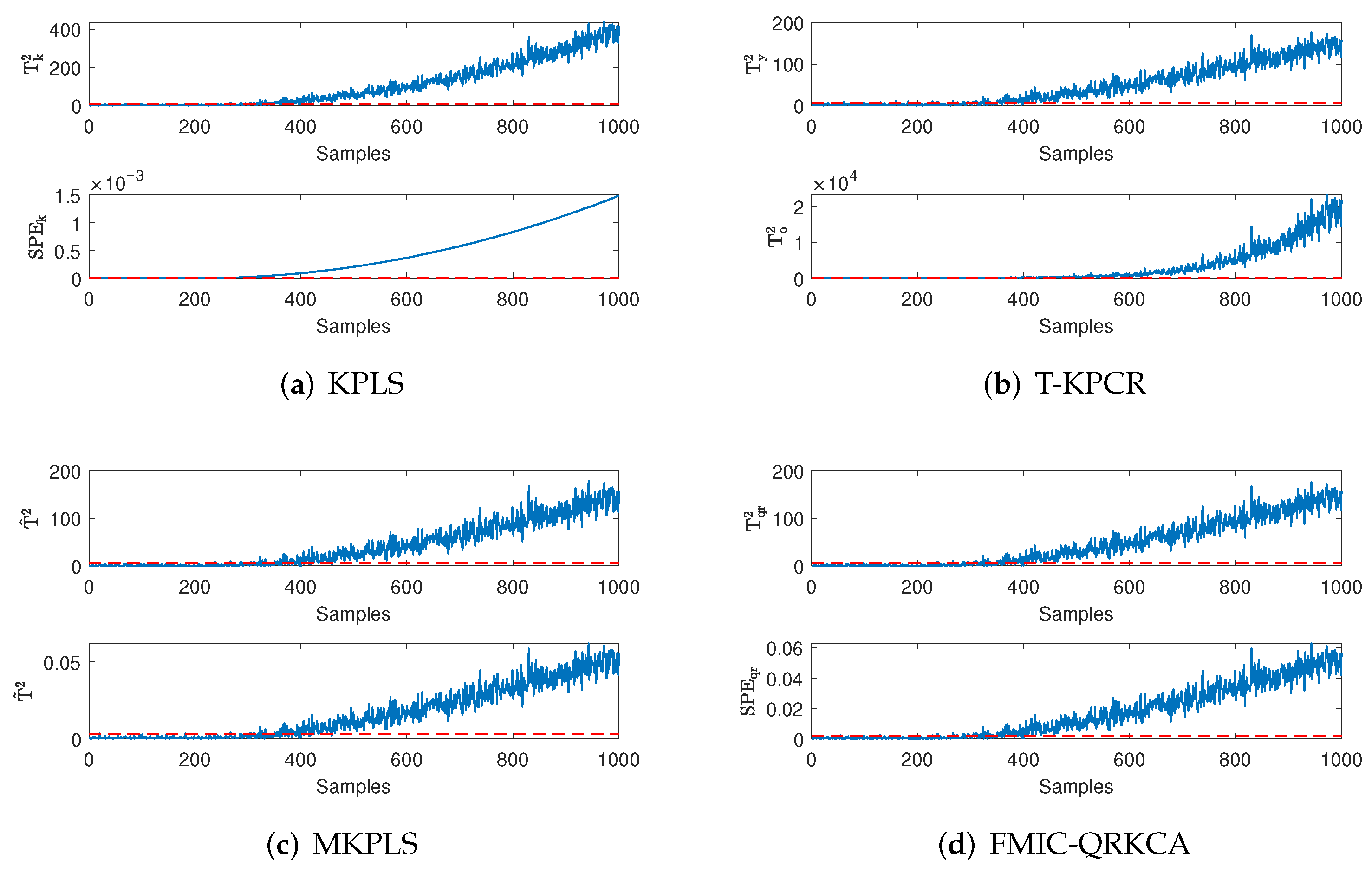
In this case, we generate 1000 normal samples to form the training dataset, and 1000 testing samples, which contain 200 normal samples and 800 fault samples, are collected to verify the performance of the methods. The parameters for the given example are set as the confidence level α = 0.99 and the kernel parameter c = 20,000. Based on the above settings, the detection performance of FMIC-QRKCA, KPLS, T-KPCR, and MKPLS methods is shown in Table 3, Table 4 and Table 5. Furthermore, the detection performance of different methods for Fault 2 s f and Fault 3 r f is shown in Figure 1 and Figure 2, respectively.
It can be seen from Table 3 that under fault-free conditions, all detection indicators of the KPLS, T-KPCR, MKPLS, and FMIC-QRKCA methods exhibit low FARs. Among these methods, the detection indicators T q r 2 and S P E q r obtained by the proposed FMIC-QRKCA method in the two subspaces have even lower FARs. Analysis of Table 4 and Figure 1 reveals critical performance distinctions. For quality-related step faults, such as Faults 1 s f and 2 s f , the KPLS, T-KPCR, MKPLS, and FMIC-QRKCA methods can accurately determine the fault types as quality-related faults through their respective detection logic. However, significant divergence emerges when handling quality-unrelated step faults, such as Faults 2 s f and 4 s f . The KPLS and T-KPCR methods exhibit diagnostic errors by misclassifying these quality-unrelated faults as quality-related. The MKPLS and FMIC-QRKCA methods can accurately determine Faults 2 s f and 4 s f as the quality-unrelated faults. Notably, the proposed FMIC-QRKCA demonstrates superior detection performance. Its S P E q r detection statistic achieves substantially lower FARs, which often reaches 0 % compared to benchmark methods. This combination of precise fault-type discrimination and minimized false alarms establishes FMIC-QRKCA as the optimal performer for step fault detection scenarios.
By observing Table 5 and Figure 2, it is obvious that for the quality-related ramp faults, such as Faults 1 r f and 3 r f , the KPLS, T-KPCR, MKPLS, and FMIC-QRKCA methods give accurate judgments for the fault types. Moreover, for the quality-unrelated ramp faults, such as Faults 2 r f and 4 r f , the KPLS and T-KPCR methods give incorrect diagnostic results; in contrast the MKPLS and FMIC-QRKCA methods can accurately determine Faults 2 r f and 4 r f as the quality-unrelated faults. Furthermore, compared with other methods, the proposed FMIC-QRKCA method has lower FARs in the quality-related subspace. Hence, for the ramp faults, the proposed FMIC-QRKCA method has excellent detection performance.

4.2. Industrial Case

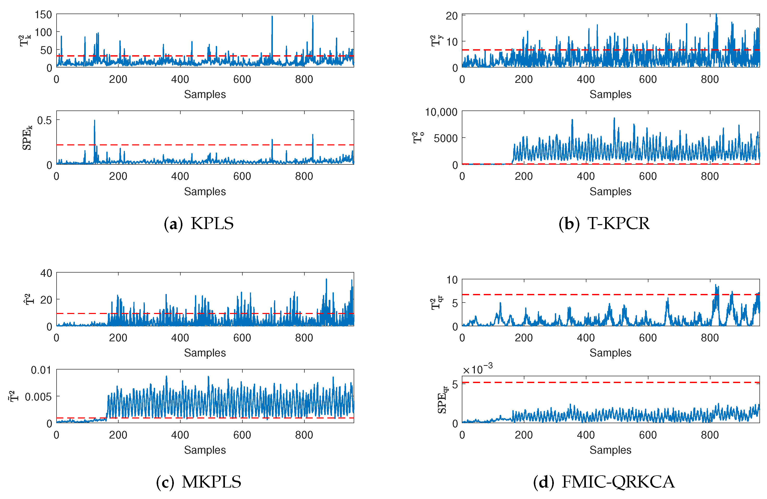
In this part, the Tennessee Eastman (TE) process is utilized to test the monitoring performance of the KPLS, T-KPCR, MKPLS, and FMIC-QRKCA methods [31]. In the TE process, the variables can be divided into two parts: the manipulated variables XMV (1–12) and the manipulated variables XMEAS (1–41). The XMEAS block contains 22 process variables and 19 analysis variables. In this part, the process space is composed of 22 process variables XMEAS (1–22) and 11 manipulated variables, XMV (1–11), and the quality space is composed of two measured variables, XMEAS (35) and XMEAS (36). The parameters of this case study are set as confidence level α = 0.99 and kernel parameter c = 20,000. Based on the above settings, the detection performance of the proposed FMIC-QRKCA method, the KPLS method, the T-KPCR method, and the MKPLS method is shown in Table 6, Table 7 and Table 8. The corresponding detection performance of different methods for these faults is shown in Figure 3 and Figure 4.
It can be seen from Table 6 that under fault-free conditions, all detection indicators of the KPLS, T-KPCR, MKPLS, and FMIC-QRKCA methods exhibit low FARs. Among these methods, the detection indicators T q r 2 and S P E q r obtained by the proposed FMIC-QRKCA method in the two subspaces have even lower FARs. For the quality-related faults in Table 7, it is clear that the T k 2 of the KPLS method, T y 2 of the T-KPCR method, T ^ 2 of the MKPLS method, and T q r 2 & S P E q r of the FMIC-QRKCA method proposed in this paper exhibit high FDRs for most faults and can diagnose them as the quality-related faults based on their respective detection logic. Among these, it is evident that for fault IDVs (1, 2, 6, 7, 8, 12, 13), the FDRs of the FMIC-QRKCA method proposed in this paper all exceed 98 % and surpass those of other methods, which undoubtedly validates that the proposed method demonstrates superior performance compared to other methods in detecting quality-related faults.
For the quality-unrelated faults listed in Table 8, these faults do not affect the quality variables XMEAS (35) and XMEAS (36). Take IDV(14) as an example: the fault of IDV(14), defined as a sudden increase in reactor feed temperature, has no impact on XMEAS (35) or XMEAS (36). The core physical reasoning is as follows: This fault manifests only as a moderate temperature disturbance in the mixed feed at the reactor inlet, and it does not alter the core reaction conditions inside the reactor. These core conditions (e.g., reaction selectivity) are determined by the catalyst, as well as intra-reactor temperature and pressure, parameters that remain unperturbed by the feed temperature fluctuation. Consequently, the propylene-to-propane component ratio at the reactor outlet stays stable. In parallel, the purity of XMEAS (35) (propylene purity) and XMEAS (36) (propane purity) is governed by the separation efficiency of the downstream C3 distillation column. This column maintains consistent separation performance via independent closed-loop control, including key parameters such as reflux ratio and column-bottom reboiler heat duty. When the column feed is free of abnormalities, the column control loop effectively mitigates minor upstream disturbances. This ensures that the final propylene and propane purity, reflected by XMEAS35 and XMEAS36, remains unaffected by the IDV(14). By observing the detection metrics within the quality-related subspace, namely the FARs of the T k 2 statistic of the KPLS method, the T y 2 statistic of the T-KPCR method, the T ^ 2 statistic of the MKPLS method, and the T q r 2 & S P E q r statistic of the proposed FMIC-QRKCA method, it is evident that for most non-quality-related faults, the MKPLS and FMIC-QRKCA methods exhibit lower FARs compared to the KPLS and T-KPCR methods. For fault IDV(14), the proposed FMIC-QRKCA method has the lowest FAR among the four methods, as shown in Figure 4. Therefore, the proposed KPCA-QoPLS method is superior to the other methods for quality-unrelated process monitoring.

4.3. Discussions

Compared with the traditional KPLS method, the proposed method inevitably increases the method complexity. However, as indicated by the above method analysis, the increased complexity is mainly concentrated in the offline phase; only the variable selection results and projection matrix obtained from offline training are required for the online detection phase. Therefore, the increased method complexity is acceptable given the rapid development of computer technology today. Furthermore, the analysis of detection performance reveals the following: For quality-related faults, the performance of the proposed method is comparable to that of the KPLS method, and both can accurately identify such faults as quality-related. For quality-unrelated faults, the KPLS method still exhibits a higher FDRs in the quality-related subspace than the FMIC-QRKCA method. It can be concluded that the proposed method is more accurate than the KPLS method in determining fault types.

5. Conclusions

In conclusion, this paper has addressed the critical challenge of quality-related fault detection in competitive industrial environments by proposing the FMIC-QRKCA methodology. Capitalizing on information fusion principles, we first developed the FMIC strategy to quantify complex correlations between process variables and multivariate quality indicators. This foundation enabled the integration of FMIC with KPCA to create the novel QRKCA method, which overcomes the fundamental limitation of conventional KPCA that neglects quality variables during principal component selection. Through rigorous validation using both numerical simulations and industrial process benchmarks, the proposed FMIC-QRKCA has demonstrated significantly superior detection accuracy for quality-related faults compared to established methods. This approach provides a robust theoretical and practical foundation for implementing intelligent quality control systems in modern industrial processes, ultimately enhancing product integrity and competitive advantage in high-stakes manufacturing environments.

Author Contributions

Conceptualization, J.Y.; methodology, J.Y. and Y.W.; software, Y.W.; validation, J.Y., Y.W. and H.M.; formal analysis, H.M.; writing—original draft preparation, J.Y.; writing—review and editing, Y.W.; supervision, H.M. All authors have read and agreed to the published version of the manuscript.

Funding

This work was supported by Wuxi Science and Technology Development Fund Project under Grant K20241048 and K20241029, and Wuxi University Research Start-up Fund for Introduced Talents under Grant 2023r020, and the Fundamental Research Funds for the Central Universities under Grant JUSRP202501036.

Data Availability Statement

The original contributions presented in this study are included in the article. Further inquiries can be directed to the corresponding author.

Conflicts of Interest

The authors declare no conflicts of interest.

References

  1. Zhou, L.; Wang, Y.; Wu, Y.; He, S.; Song, Z. Quality-relevant modeling and monitoring of industrial cyber-physical systems: The semi-supervised dynamic latent variable models. IEEE Trans. Ind. Cyber-Phys. Syst. 2024, 3, 39–47. [Google Scholar] [CrossRef]
  2. Zhang, X.; Ma, L.; Peng, K.; Zhang, C.; Shahid, M.A. A cloud–edge collaboration based quality-related hierarchical fault detection framework for large-scale manufacturing processes. Expert Syst. Appl. 2024, 256, 124909. [Google Scholar] [CrossRef]
  3. Yang, Y.; Ding, S.X.; Li, L. On observer-based fault detection for nonlinear systems. Syst. Control Lett. 2015, 82, 18–25. [Google Scholar] [CrossRef]
  4. Yu, W.; Zhao, C.; Huang, B.; Xie, M. Intrinsic causality embedded concurrent quality and process monitoring strategy. IEEE Trans. Ind. Electron. 2024, 71, 15111–15121. [Google Scholar] [CrossRef]
  5. Zhao, Z.; Huang, J.; Zhang, M.; Zhang, J. Dynamic event-triggered interval observer-based fault detection for a class of nonlinear cyber-physical systems with disturbance. Axioms 2025, 14, 435. [Google Scholar] [CrossRef]
  6. Wang, Z.; Wang, C.; Li, Y. Variational autoencoder based on knowledge sharing and correlation weighting for process-quality concurrent fault detection. Eng. Appl. Artif. Intell. 2024, 133, 108051. [Google Scholar] [CrossRef]
  7. Liu, Q.; Zhu, Q.; Qin, S.J.; Chai, T. Dynamic concurrent kernel cca for strip-thickness relevant fault diagnosis of continuous annealing processes. J. Process Control 2018, 67, 12–22. [Google Scholar] [CrossRef]
  8. Jafari, N.; Lopes, A.M. Fault detection and identification with kernel principal component analysis and long short-term memory artificial neural network combined method. Axioms 2023, 12, 583. [Google Scholar] [CrossRef]
  9. Chen, Z.; Cao, Y.; Ding, S.X.; Zhang, K.; Koenings, T.; Peng, T.; Yang, C.; Gui, W. A distributed canonical correlation analysis-based fault detection method for plant-wide process monitoring. IEEE Trans. Ind. Inform. 2019, 15, 2710–2720. [Google Scholar] [CrossRef]
  10. Shah, M.Z.H.; Ahmed, Z.; Lisheng, H. Weighted linear local tangent space alignment via geometrically inspired weighted pca for fault detection. IEEE Trans. Ind. Inform. 2022, 19, 210–219. [Google Scholar] [CrossRef]
  11. Hu, C.; Luo, J.; Kong, X.; Xu, Z. Orthogonal multi-block dynamic pls for quality-related process monitoring. IEEE Trans. Autom. Sci. Eng. 2024, 21, 3421–3434. [Google Scholar] [CrossRef]
  12. Liu, D.; Shang, J.; Chen, M. Principal component analysis-based ensemble detector for incipient faults in dynamic processes. IEEE Trans. Ind. Inform. 2020, 17, 5391–5401. [Google Scholar] [CrossRef]
  13. Chen, Z.; Liu, C.; Ding, S.X.; Peng, T.; Yang, C.; Gui, W.; Shardt, Y.A. A just-in-time-learning-aided canonical correlation analysis method for multimode process monitoring and fault detection. IEEE Trans. Ind. Electron. 2020, 68, 5259–5270. [Google Scholar] [CrossRef]
  14. Dong, Y.; Qin, S.J. Regression on dynamic pls structures for supervised learning of dynamic data. J. Process Control 2018, 68, 64–72. [Google Scholar] [CrossRef]
  15. Sun, R.; Wang, Y. Key-performance-indicator-related fault detection based on deep orthonormal subspace analysis. IEEE Trans. Ind. Inform. 2024, 20, 7249–7258. [Google Scholar] [CrossRef]
  16. Wang, G.; Jiao, J.; Yin, S. A kernel direct decomposition-based monitoring approach for nonlinear quality-related fault detection. IEEE Trans. Ind. Inform. 2016, 13, 1565–1574. [Google Scholar] [CrossRef]
  17. Si, Y.; Wang, Y.; Zhou, D. Key-performance-indicator-related process monitoring based on improved kernel partial least squares. IEEE Trans. Ind. Electron. 2020, 68, 2626–2636. [Google Scholar] [CrossRef]
  18. Jiao, J.; Zhen, W.; Zhu, W.; Wang, G. Quality-related root cause diagnosis based on orthogonal kernel principal component regression and transfer entropy. IEEE Trans. Ind. Inform. 2020, 17, 6347–6356. [Google Scholar] [CrossRef]
  19. Wang, G.; Yang, J.; Qian, Y.; Han, J.; Jiao, J. Kpca-cca-based quality-related fault detection and diagnosis method for nonlinear process monitoring. IEEE Trans. Ind. Inform. 2022, 19, 6492–6501. [Google Scholar] [CrossRef]
  20. Sun, C.; Yin, Y.; Kang, H.; Ma, H. A distributed principal component regression method for quality-related fault detection and diagnosis. Inf. Sci. 2022, 600, 301–322. [Google Scholar] [CrossRef]
  21. Chen, Q.; Liu, Z.; Ma, X.; Wang, Y. Artificial neural correlation analysis for performance-indicator-related nonlinear process monitoring. IEEE Trans. Ind. Inform. 2021, 18, 1039–1049. [Google Scholar] [CrossRef]
  22. Zhou, D.; Li, G.; Qin, S.J. Total projection to latent structures for process monitoring. AIChE J. 2010, 56, 168–178. [Google Scholar] [CrossRef]
  23. Peng, K.; Zhang, K.; Li, G. Quality-related process monitoring based on total kernel PLS model and its industrial application. Math. Probl. Eng. 2013, 2013, 707953. [Google Scholar] [CrossRef]
  24. Wang, G.; Luo, H.; Peng, K. Quality-related fault detection using linear and nonlinear principal component regression. J. Frankl. Inst. 2016, 353, 2159–2177. [Google Scholar] [CrossRef]
  25. Jiao, J.; Zhao, N.; Wang, G.; Yin, S. A nonlinear quality-related fault detection approach based on modified kernel partial least squares. ISA Trans. 2017, 66, 275–283. [Google Scholar] [CrossRef]
  26. Wang, Y.; Zhou, D.; Chen, M. Dynamic related component analysis for quality-related process monitoring with applications to thermal power plants. Control Eng. Pract. 2023, 132, 105426. [Google Scholar] [CrossRef]
  27. Wang, Y.; Zhou, D.; Chen, M.; Wang, M. Weighted part mutual information related component analysis for quality-related process monitoring. J. Process Control 2020, 88, 111–123. [Google Scholar] [CrossRef]
  28. Song, B.; Shi, H.; Tan, S.; Tao, Y. Multisubspace orthogonal canonical correlation analysis for quality-related plant-wide process monitoring. IEEE Trans. Ind. Inform. 2020, 17, 6368–6378. [Google Scholar] [CrossRef]
  29. Zhang, C.; Peng, K.; Dong, J.; Zhang, X. Kpi-related operating performance assessment based on distributed imrmr-kocta for hot strip mill process. Expert Syst. Appl. 2022, 209, 118273. [Google Scholar] [CrossRef]
  30. Reshef, D.N.; Reshef, Y.A.; Finucane, H.K.; Grossman, S.R.; McVean, G.; Turnbaugh, P.J.; Lander, E.S.; Mitzenmacher, M.; Sabeti, P.C. Detecting novel associations in large data sets. Science 2011, 334, 1518–1524. [Google Scholar] [CrossRef]
  31. McAvoy, T.J. A plant-wide industrial process control problem. Comput. Chem. Eng. 1993, 17, 245–255. [Google Scholar] [CrossRef]
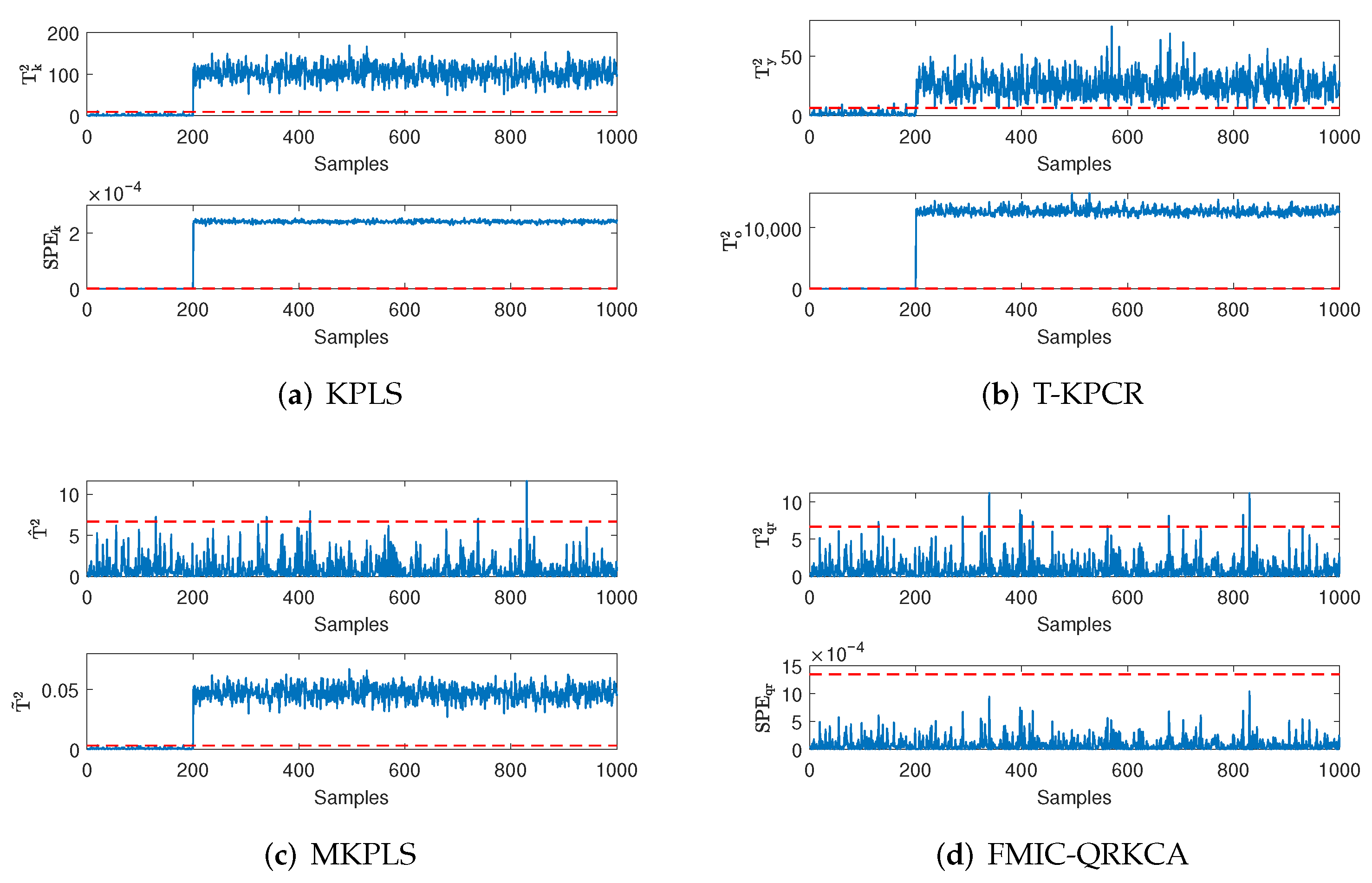
Figure 1. Detection results of different methods for the quality-unrelated step fault Fault 2 s f .
Axioms 14 00745 g001
Figure 2. Detection results of different methods for the quality-related step fault Fault 3 s f .
Axioms 14 00745 g002
Figure 3. Monitoring results of different methods for IDV(12).
Axioms 14 00745 g003
Figure 4. Monitoring results of different methods for IDV(14).
Axioms 14 00745 g004
Table 1. Quality-related fault detection based on the FMIC-QRKCA method.
Offline modeling:
(1)
Normalize the process and quality matrices X and Y .
(2)
Based on the proposed FMIC method and the quality variable Y , complete the preselection of process variables X , obtain the quality-related part X q r , and retain the corresponding variable labels.
(3)
Using the selected X q r , calculate the kernel matrix and perform mean normalization to obtain K ¯ .
(4)
Perform eigenvalue decomposition on the obtained K ¯ to obtain the eigenvalues λ i and their corresponding eigenvectors β i .
(5)
Construct the projection matrix B using the obtained eigenvectors β i .
(6)
Using the obtained projection matrix B , calculate the entire principal component space T .
(7)
Based on the FMIC method and the quality variable Y , extract the high-quality-related principal component T q r in the principal component space and retain the corresponding label.
(8)
Calculate the detection thresholds J t h , T q r 2 and J t h , s p e q r for the T 2 statistic and the S P E q r statistic.
Online detection:
(9)
Normalize the new process variable vector x n e w .
(10)
Based on the variable labels corresponding to X q r obtained offline, perform variable screening on x n e w to obtain x n e w , q r .
(11)
Calculate the kernel vector k ¯ n e w , q r using x n e w , q r .
(12)
Calculate the principal component vector t n e w of the new data based on the obtained projection matrix B .
(13)
Based on the variable labels corresponding to T q r obtained offline, perform variable screening on t n e w to obtain t n e w , q r .
(14)
Calculate the T q r 2 and S P E q r statistics of the new data, respectively.
(15)
Based on the detection logic, determine the fault types.
Table 2. Fault types.
VariableStep Fault ( f = 0.2 )Ramp Fault ( f = 0.0006 )
x 1 Fault 1 s f : x 1 = x 1 n o r + f Fault 1 r f : x 1 = x 1 n o r + ( s 200 ) f ( 201 s 1000 )
x 2 Fault 2 s f : x 2 = x 2 n o r + f Fault 2 r f : x 2 = x 2 n o r + ( s 200 ) f ( 201 s 1000 )
x 3 Fault 3 s f : x 3 = x 3 n o r + f Fault 3 r f : x 3 = x 3 n o r + ( s 200 ) f ( 201 s 1000 )
x 4 Fault 4 s f : x 4 = x 4 n o r + f Fault 4 r f : x 4 = x 4 n o r + ( s 200 ) f ( 201 s 1000 )
Table 3. FARs of the KPLS, T-KPCR, MKPLS, and FMIC-QRKCA methods under fault-free condition.
Fault TypesKPLST-KPCRMKPLSFMIC-QRKCA
T k 2 SPE k T y 2 T o 2 T ^ 2 T ˜ 2 T qr 2 SPE qr
faut-free1.250.754.133.871.131.371.120
Table 4. FDRs of the KPLS, T-KPCR, MKPLS, and FMIC-QRKCA methods for the step faults.
Fault TypesKPLST-KPCRMKPLSFMIC-QRKCA
T k 2 SPE k T y 2 T o 2 T ^ 2 T ˜ 2 T qr 2 SPE qr
Fault 1 s f 100100100100100100100100
Fault 2 s f 10010099.251000.51001.120
Fault 3 s f 10010010010099.7510010098.38
Fault 4 s f 1001001001000.6251001.120
Table 5. FDRs of the KPLS, T-KPCR, MKPLS, and FMIC-QRKCA methods for the ramp faults.
Fault TypesKPLST-KPCRMKPLSFMIC-QRKCA
T k 2 SPE k T y 2 T o 2 T ^ 2 T ˜ 2 T qr 2 SPE qr
Fault 1 r f 88.6299.3884.8899.2592.379191.8887.85
Fault 2 r f 88.5099.1279.8799.12191.2510
Fault 3 r f 85.3899.0082.8796.1380.1279.8781.8773.62
Fault 4 r f 88.1298.7588.8898.25181.251.120.00
Table 6. FARs of the KPLS, T-KPCR, MKPLS, and FMIC-QRKCA methods under fault-free condition in the TE prcoess.
Fault TypesKPLST-KPCRMKPLSFMIC-QRKCA
T k 2 SPE k T y 2 T o 2 T ^ 2 T ˜ 2 T qr 2 SPE qr
faut-free1.160.559.517.371.2511.376.120
Table 7. FDRs of different methods under the quality-related faults.
FaultDefinitionKPLST-KPCRMKPLSFMIC-QRKCA
T k 2 T y 2 T ^ 2 T qr 2 & SPE qr
IDV(1)A/C feed ratio, B composition constant (Stream 4)95.1365.7591.7599.88
IDV(2)B composition A/C ration constant (Streams 4)96.1395.5055.8898.88
IDV(5)Condenser cooling water inlet temperature34.8829.7510.3730.12
IDV(6)Reactor feed rate99.3899.6296.1299.50
IDV(7)Reactor cooling water inlet temperature50.2570.3720.63100
IDV(8)A, B, C feed composition (Stream 4)94.5090.6265.0098.25
IDV(12)Condenser cooling water inlet temperature93.0094.0062.5099.00
IDV(13)Reaction kinetics95.0090.7578.5095.50
Table 8. FDRs of different methods under the quality-unrelated faults.
FaultDefinitionKPLST-KPCRMKPLSFMIC-QRKCA
T k 2 T y 2 T ^ 2 T qr 2 & SPE qr
IDV(3)D feed temperature (Stream 2)1710.370.636.75
IDV(4)Reactor cooling water inlet temperature1513.500.756.88
IDV(9)D Feed temperature14.259.250.754.50
IDV(11)Reactor cooling water inletting water inlet temperature18.1215.502.7510.62
IDV(14)Reactor cooling water inlet temperature6.3816.6313.631.38
IDV(15)Condenser cooling water valve17.2514.505.510.62
Disclaimer/Publisher’s Note: The statements, opinions and data contained in all publications are solely those of the individual author(s) and contributor(s) and not of MDPI and/or the editor(s). MDPI and/or the editor(s) disclaim responsibility for any injury to people or property resulting from any ideas, methods, instructions or products referred to in the content.