Article

Stability of the Split-Step θ-Method for Stochastic Pantograph Systems with Markovian Switching and Jumps

1
School of Mathematics and Statistics, Guangdong University of Foreign Studies, Guangzhou 510006, China
2
School of Automation Science and Engineering, South China University of Technology, Guangzhou 510641, China
3
School of Automation, Guang Dong Polytechnic Normal University, Guangzhou 510665, China
*
Author to whom correspondence should be addressed.
Axioms 2025, 14(10), 718; https://doi.org/10.3390/axioms14100718
Submission received: 16 August 2025 / Revised: 15 September 2025 / Accepted: 22 September 2025 / Published: 23 September 2025

Abstract

This study focuses on analyzing the almost sure exponential stability of the split-step θ -method ( S S θ -method) when applied to stochastic pantograph differential equations characterized by Markovian switching and jump processes. Initially, we establish the almost sure exponential stability of the system’s trivial solution. Subsequently, under an additional sufficient condition, it is demonstrated that the discrete solutions generated by the S S θ -method also exhibit this stability property. Finally, a computational experiment is conducted to support the theoretical results.

1. Introduction

In practice, many stochastic systems exhibit dependence not only on their present conditions but also on historical dynamics. To effectively characterize such behavior, stochastic delay differential equations (SDDEs) are widely utilized (see, for instance, [1,2,3,4,5,6]). When these systems experience sudden shifts in configuration or parameter values, it becomes appropriate to employ SDDEs incorporating Markovian switching, as discussed in the comprehensive work [7]. Mao et al. [8] studied the exponential stability of SDDEs with Markovian switching. Song and Zhu [9] examined the asymptotic stability in mean square, stochastic stability, and exponential stability in mean square of linear SDDEs with infinite Markovian switchings. Subsequently, Zhang and Chen [10] investigated the stability of SDDEs with Markovian switching. While Brownian motion is a well-known model for continuous stochastic processes, it may not adequately capture random discontinuities caused by events like mechanical breakdowns, seismic activity, or extreme weather. In these cases, modeling with jump processes provides a more suitable representation. Accordingly, SDDEs that integrate both Markovian switching and jump disturbances have become an area of active research, with detailed investigations reported in [11,12] and numerous references therein.
Pantograph equations, a distinctive subclass of delay differential systems, were originally introduced in the context of modeling electric locomotives, as documented in [13]. With the integration of stochastic analysis, stochastic pantograph differential equations (SPDEs) have emerged as essential tools in disciplines such as mechanics, biology, engineering, and financial mathematics [14]. Fan et al. showed sufficient conditions of existence and uniqueness of the solutions for SPDEs in [15] and studied the stability in [16]. Jang et al. [17] conducted further research into the asymptotic stability of SPDEs with Markovian switching. Milošević [18] discussed the existence, uniqueness and almost sure polynomial stability of solutions to a class of highly nonlinear SPDEs, as well as the corresponding Euler–Maruyama approximation. For these above-mentioned foundational results regarding the existence, uniqueness, and stability of solutions to SPDEs, readers can further refer to other relevant literature. The work of You et al. [19] addresses the almost sure exponential stability of SPDEs influenced by Markovian switching mechanisms. Furthermore, Mao and collaborators [20] extended the analysis to neutral SPDEs, examining their almost sure exponential stability under general decay conditions in the presence of Markovian switching.
However, most of SPDEs cannot be solved explicitly. Especially, explicit solutions can rarely be obtained for nonlinear SPDEs. As a result, numerical approximation techniques have become essential tools for their analysis (see, e.g., [21,22]). Notably, Zhou and Hu [23] examined the almost sure exponential stability of the backward Euler–Maruyama scheme when applied to SPDEs governed by Markovian switching. In another study, Guo and Li [24] evaluated both the Euler–Maruyama and the backward Euler–Maruyama methods, demonstrating the almost sure exponential stability of their numerical solutions. In [25], Cheng et al. focused on the strong convergence and stability of the balanced Euler scheme for SPDEs with regime-switching behavior. A notable development in numerical schemes for stochastic differential equations was put forward by Ding et al. [26], who proposed the so-called S S θ -scheme. This method has since attracted significant scholarly attention. For instance, Huang [27] studied the mean-square stability properties of the S S θ -scheme in the context of SDDEs. Similarly, the work in [28] established conditions under which the S S θ -scheme guarantees mean-square stability for SDDEs under mild assumptions. Mo et al. [29] demonstrated that the S S θ -scheme ensures mean-square exponential stability of the zero solution in neutral SDDEs affected by jump processes. In [30], Yuan et al. verified the asymptotic mean-square stability for the same class of equations. Moreover, Xiao et al. [31] investigated how adaptive time-stepping strategies influence the mean-square stability of the S S θ -scheme when applied to SPDEs. Guo and Li [32] further explored the almost sure exponential stability of two variants of theta-type numerical schemes tailored for SPDEs.
Despite the significant advancements in the study of S S θ -methods, existing research has yet to explore their almost sure stability when applied to SPDEs featuring both Markovian switching and jump disturbances (SPDEwMJs). Consequently, it becomes essential to examine the stability characteristics of such systems using the S S θ -framework. This work initially demonstrates the almost sure exponential stability of the zero solution to a representative SPDEwMJ. Following this, we establish that the proposed S S θ -based numerical scheme maintains this stability under an additional, suitably chosen condition.
The rest of the present article is structured in the following manner. Section 2 outlines the foundational conceptions and notation required for the subsequent analysis. Section 3 focuses on establishing the almost sure exponential stability of both the exact solution and the numerical approximation derived via the S S θ -method. Section 4 presents a concrete example for illustrating and validating the theoretical findings. Lastly, this work concludes by presenting a concise summary of its key findings.

2. Preliminaries

Throughout the present article, the following notations are adopted. Denote R = ( , + ) and R + = [ 0 , + ) . For all x R , x stands for the greatest integer not exceeding x. The space R n is referred to as the n-dimensional Euclidean space, where | x | denotes the Euclidean norm for any vector x R n . Let ( Ω , F , P ) be a complete probability space, accompanied by a filtration { F t } t 0 satisfying the usual conditions (i.e., right-continuity and completeness). We consider a right-continuous Markov chain { r ( t ) } t 0 defined on ( Ω , F , P ) , taking values in a finite set S = { 1 , 2 , , N } . The infinitesimal generator of this Markov process is denoted by the matrix Γ = ( γ i j ) N × N with
P { r ( t + Δ ) = j | r ( t ) = i } = γ i j Δ + o ( Δ ) , if i j , 1 + γ i i Δ + o ( Δ ) , if i = j ,
where Δ > 0 , with lim Δ 0 o ( Δ ) Δ = 0 ; for i j , γ i j 0 denotes the transition rate from state i to state j, whereas γ i i = j i γ i j . For the properties of r ( t ) , reference may be made to [7].
Consider the following SPDEwMJ, which takes the form
d x ( t ) = f ( x ( t ) , x ( q t ) , r ( t ) , t ) d t + g ( x ( t ) , x ( q t ) , r ( t ) , t ) d ω ( t ) + h ( x ( t ) , x ( q t ) , r ( t ) , t ) d N ( t ) , t 0
with initial conditions x ( 0 ) = x 0 and r ( 0 ) = i 0 S ; here, 0 < q < 1 , the functions f , g , h are defined as mappings from R n × R n × S × R + to R n . It is assumed that x 0 is a bounded, F 0 -measurable random variable. Let ω ( t ) denote a one-dimensional standard Brownian motion, and let N ( t ) be a scalar Poisson process with intensity λ > 0 . The compensated Poisson process is defined by N ˜ ( t ) = N ( t ) λ t . Furthermore, the processes ω ( t ) , N ( t ) , and r ( t ) are mutually independent. To support the stability analysis, we impose the assumption that f ( 0 , 0 , i , t ) = g ( 0 , 0 , i , t ) = h ( 0 , 0 , i , t ) = 0 , f o r a l l ( i , t ) S × R + , which guarantees that Equation (1) admits the trivial solution.
Throughout the paper, the following hypotheses are assumed to be satisfied:
Hypothesis 1 (H1).
For any integer α 1 , there exists a constant L α > 0 with the property that for all x 1 , x 2 , y 1 , y 2 R n , i S , and t R + , the following inequality holds
max { | f ( x 1 , y 1 , i , t ) f ( x 2 , y 2 , i , t ) | 2 , | g ( x 1 , y 1 , i , t ) g ( x 2 , y 2 , i , t ) | 2 , | h ( x 1 , y 1 , i , t ) h ( x 2 , y 2 , i , t ) | 2 } L α | x 1 x 2 | 2 + | y 1 y 2 | 2 .
for any i S , t R + and x j , y j R n with | x j | | y j | α (j = 1, 2).
Hypothesis 2 (H2).
There exist constants λ 1 > 0 and λ 2 > 0 with the property that for all x , y R n , i S , and t R + , the following inequality is satisfied:
| h ( x , y , i , t ) | 2 λ 1 | x | 2 + λ 2 q e ( 1 q ) t | y | 2 .
To prove the existence and uniqueness of solutions to Equation (1), we introduce the following notation. Let C 2 , 1 ( R n × R + ; R + ) denote the class of real-valued functions V ( x , t ) : R n × R + R + that are twice continuously differentiable with respect to x and once with respect to t. For any V C 2 , 1 ( R n × R + ; R + ) , define the associated operator L V : R n × R n × S × R + R as
L V ( x , y , i , t ) = V t ( x , t ) + V x ( x , t ) f ( x , y , i , t ) + 1 2 trace g ( x , y , i , t ) V x x ( x , t ) g ( x , y , i , t ) + λ V ( x + h ( x , y , i , t ) , t ) V ( x , t ) + j = 1 N γ i j V ( x , t ) .
where V t ( x , t ) = V ( x , t ) t , V x ( x , t ) = V ( x , t ) x i 1 × n , V x x ( x , t ) = 2 V ( x , t ) x i x j n × n .
Theorem 1. 
Suppose that assumptions (H1) and (H2) are satisfied. Further, assume there exist positive constants λ 3 and λ 4 such that the following inequality is valid for all x , y R n and ( i , t ) S × R + :
2 x T f ( x , y , i , t ) + | g ( x , y , i , t ) | 2 λ 3 | x | 2 + λ 4 q e ( 1 q ) t | y | 2 .
If, in addition, the inequality λ 3 > λ 4 + λ ( 1 + 2 λ 1 + 2 λ 2 ) is satisfied, then for any initial data x 0 R n and i 0 S , Equation (1) admits a unique global solution x ( t ) defined on the entire interval t R + .
Proof. 
Let V ( x ( t ) , t ) = | x ( t ) | 2 . Applying Itô’s formula to | x ( t ) | 2 , it can be derived that for any i S and t 0 ,
L V ( x , y , i , t ) = 2 x T f ( x , y , i , t ) + | g ( x , y , i , t ) | 2 + λ [ | h ( x , y , i , t ) | 2 + 2 x T h ( x , y , i , t ) ] 2 x T f ( x , y , i , t ) + | g ( x , y , i , t ) | 2 + λ [ | x | 2 + 2 | h ( x , y , i , t ) | 2 ] .
It can be inferred from Equations (3) and (4) that one gains
L V ( x , y , i , t ) [ λ 3 λ ( 1 + 2 λ 1 ) ] | x | 2 + ( λ 4 + 2 λ λ 2 ) q e ( 1 q ) t | y | 2 .
By combining Inequality (4) with the condition λ 3 > λ 4 + λ ( 1 + 2 λ 1 + 2 λ 2 ) , and applying reasoning similar to that used in the proof of Theorem 2.3 (1) in You et al. [19], it follows that Equation (1) is endowed with a unique global solution x ( t ) for all t 0 . □
Next, the S S θ -method applied to Equation (1) will be discussed. Before discussing it, we invoke the following lemma:
Lemma 1 
([7] (p. 112)). Let Δ > 0 , and define r k Δ = r ( k Δ ) for all integers k 0 . Then the sequence { r k Δ , k = 0 , 1 , 2 , } forms a discrete-time Markov chain whose one-step transition probability matrix is given by
p ( Δ ) = ( p i j ( Δ ) ) N × N = e Δ Γ .
Given a fixed step size Δ > 0 , the discrete Markov chain { r k Δ } k = 0 can be generated using the following simulation procedure: First, compute the transition probability matrix using Equation (6). Set the initial value r 0 Δ = i 0 , and generate a uniform random variable ξ 1 U ( 0 , 1 ) . Then define
r 1 Δ = i 1 , if i 1 S { N } satisfies j = 1 i 1 1 p i 0 , j ( Δ ) ξ 1 < j = 1 i 1 p i 0 , j ( Δ ) , N , if j = 1 N 1 p i 0 , j ( Δ ) ξ 1 ,
with the convention j = 1 0 p i 0 , j ( Δ ) = 0 . Repeat the process by generating another independent uniform random number ξ 2 U ( 0 , 1 ) , and define
r 2 Δ = i 2 , if i 2 S { N } satisfies j = 1 i 2 1 p r 1 Δ , j ( Δ ) ξ 2 < j = 1 i 2 p r 1 Δ , j ( Δ ) , N , if j = 1 N 1 p r 1 Δ , j ( Δ ) ξ 2 .
By iterating this process, one obtains a complete trajectory { r k Δ } k = 0 , and independent realizations can be generated as needed for simulation purposes.
With the discrete Markov chain construction established, we now introduce the S S θ -method for numerically solving Equation (1). Let t k = k Δ for k Z + and select a parameter θ [ 0 , 1 ] . Starting from initial values ( y 0 , r 0 Δ ) = ( x 0 , i 0 ) , the numerical scheme is defined as follows:
u k = y k + θ f ( u k , u q k , r k Δ , t k ) Δ , y k + 1 = y k + f ( u k , u q k , r k Δ , t k ) Δ + g ( u k , u q k , r k Δ , t k ) Δ ω k + h ( u k , u q k , r k Δ , t k ) Δ N k ,
where y k and u k are numerical approximations to the solution x ( t k ) , Δ ω k = ω ( t k + 1 ) ω ( t k ) , Δ N k = N ( t k + 1 ) N ( t k ) , and r k Δ = r ( t k ) as previously defined.
When θ = 0 , Scheme (7) reduces to the classical Euler–Maruyama method, whereas θ = 1 yields the split-step backward Euler variant.
At the end of this section, we formulate the almost sure exponential stability for both the trivial solution x ( t ) and the approximate solution y k of Equation (1).
Definition 1. 
Let the initial condition x 0 be bounded and i 0 S .
(1) 
The trivial solution of Equation (1) is referred to as almost surely exponentially stable in the sense that there exists a constant ε > 0 satisfying
lim sup t log | x ( t ) | t ε a . s .
(2) 
The numerical approximation y k , generated by Scheme (7), is referred to as almost surely exponentially stable when there exists a constant η > 0 satisfying
lim sup k log | y k | k Δ η a . s .

3. Almost Sure Exponential Stability of the Trivial Solution and the SS θ -Method

This section aims to establish the almost sure exponential stability of both the trivial solution and its corresponding numerical approximation via the S S θ -method for Equation (1).
The following theorem provides a rigorous statement regarding the almost sure exponential stability of the trivial solution x ( t ) .
Theorem 2. 
Presuming that (H1)–(H2) and Inequality (4) are valid. If λ 3 > λ 4 + λ ( 1 + 2 λ 1 + 2 λ 2 ) holds, then the trivial solution x ( t ) to Equation (1), starting from any bounded initial value x 0 R n and i 0 S , satisfies
lim sup t log | x ( t ) | t ε 2 a . s . ,
where ε = 1 λ 3 λ 4 λ ( 1 + 2 λ 1 + 2 λ 2 ) .
Proof. 
Using the Itô’s formula to e ε t | x ( t ) | 2 yields
d e ε t | x ( t ) | 2 = ε e ε t | x ( t ) | 2 d t + e ε t 2 x ( t ) f ( x ( t ) , x ( q t ) , r ( t ) , t ) + | g ( x ( t ) , x ( q t ) , r ( t ) , t ) | 2 d t + 2 e ε t x ( t ) g ( x ( t ) , x ( q t ) , r ( t ) , t ) d ω ( t ) + e ε t | x ( t ) + h ( x ( t ) , x ( q t ) , r ( t ) , t ) | 2 | x ( t ) | 2 d N ( t ) .
Using the decomposition N ( t ) = N ˜ ( t ) + λ t , one integrates both sides to obtain
e ε t | x ( t ) | 2 = | x 0 | 2 + ε 0 t e ε s | x ( s ) | 2 d s + 0 t e ε s 2 x ( s ) f ( x ( s ) , x ( q s ) , r ( s ) , s ) + | g ( x ( s ) , x ( q s ) , r ( s ) , s ) | 2 d s + λ 0 t e ε s | x ( s ) + h ( x ( s ) , x ( q s ) , r ( s ) , s ) | 2 | x ( s ) | 2 d s + 2 0 t e ε s x ( s ) g ( x ( s ) , x ( q s ) , r ( s ) , s ) d ω ( s ) + 0 t e ε s | x ( s ) + h ( x ( s ) , x ( q s ) , r ( s ) , s ) | 2 | x ( s ) | 2 d N ˜ ( s ) .
Define the local martingale M ( t ) by
M ( t ) = 2 0 t e ε s x ( s ) g ( x ( s ) , x ( q s ) , r ( s ) , s ) d ω ( s ) + 0 t e ε s | x ( s ) + h ( x ( s ) , x ( q s ) , r ( s ) , s ) | 2 | x ( s ) | 2 d N ˜ ( s )
with M ( 0 ) = 0 . Invoking inequalities in Equations (3) and (4) and the elementary estimate 2 x ( s ) h ( · ) | x ( s ) | 2 + | h ( · ) | 2 , one deduces
e ε t | x ( t ) | 2 | x 0 | 2 + 0 t e ε s ε λ 3 + λ ( 1 + 2 λ 1 ) | x ( s ) | 2 d s + q 0 t e ε s λ 4 + 2 λ λ 2 e ( 1 q ) s | x ( q s ) | 2 d s + M ( t ) .
By performing a change of variable in the delay term and bounding | x ( q s ) | 2 in terms of | x ( s ) | 2 , one can further write
e ε t | x ( t ) | 2 | x 0 | 2 + 0 t e ε s ε λ 3 + λ ( 1 + 2 λ 1 ) | x ( s ) | 2 d s + 0 t e ( ε 1 + q ) s / q λ 4 + 2 λ λ 2 | x ( s ) | 2 d s + M ( t ) .
It follows from ε = 1 { λ 3 λ 4 λ ( 1 + 2 λ 1 + 2 λ 2 ) } that one derives ε 1 , thus e ( ε 1 + q ) s / q e ε s . Then,
e ε t | x ( t ) | 2 | x 0 | 2 + 0 t e ε s [ ε λ 3 + λ 4 + λ ( 1 + 2 λ 1 + 2 λ 2 ) ] | x ( s ) | 2 d s + M ( t ) | x 0 | 2 + M ( t ) .
Thanks to the non-negative semi-martingale convergence theorem [7] (Theorem 1.1.10), it follows that
lim sup t e ε t | x ( t ) | 2 < .
Denote ρ = lim sup t e ε t | x ( t ) | 2 < . Then, for any fixed ϵ ˜ > 0 , there exists a time T ( ϵ ˜ , ρ ) > 0 such that for all t > T ( ϵ ˜ , ρ ) , one has e ε t | x ( t ) | 2 < ρ + ϵ ˜ . Taking logarithms yields ε t + 2 log | x ( t ) | log ( ρ + ϵ ˜ ) , which implies Equation (10). The proof is complete. □
We now turn our attention to analyzing the almost sure exponential stability of the numerical solution y k .
Theorem 3. 
Given that all the conditions outlined in Theorem 2 are fulfilled. Additionally, for all ( x , y , i , t ) R n × R n × S × R + , suppose the function f ( x , y , i , t ) satisfies
| f ( x , y , i , t ) | 2 λ 5 | x | 2 + λ 6 q e ( 1 q ) t | y | 2 ,
where λ 5 , λ 6 > 0 . Define
ε = min 1 , λ 3 2 λ λ 1 λ q 1 q + 1 ( λ 4 + 2 λ λ 2 ) ,
with λ 3 > 2 λ λ 1 + λ + q 1 q + 1 ( λ 4 + 2 λ λ 2 ) . Consequently, for any given δ ( 0 , ε / 2 ) , there is a positive constant Δ ¯ such that for all step sizes Δ ( 0 , Δ ¯ ] and any x 0 that is bounded and F 0 -measurable, the numerical solution y k produced by Scheme (7) satisfies
lim sup k log | y k | k Δ ε 2 + δ a . s .
That is, the S S θ -method preserves the almost sure exponential stability of Equation (1).
Proof. 
It follows from Equation (7) that yields
| y k + 1 | 2 = | y k + f ( u k , u q k , r k Δ , t k ) Δ + g ( u k , u q k , r k Δ , t k ) Δ ω k + h ( u k , u q k , r k Δ , t k ) Δ N k | 2 = | y k | 2 + | f ( u k , u q k , r k Δ , t k ) | 2 Δ 2 + | g ( u k , u q k , r k Δ , t k ) | 2 | Δ ω k | 2 + | h ( u k , u q k , r k Δ , t k ) | 2 | Δ N k | 2 + 2 y k , f ( u k , u q k , r k Δ , t k ) Δ + 2 y k + f ( u k , u q k , r k Δ , t k ) Δ , h ( u k , u q k , r k Δ , t k ) Δ N k + 2 y k + f ( u k , u q k , r k Δ , t k ) Δ , g ( u k , u q k , r k Δ , t k ) Δ ω k + 2 g ( u k , u q k , r k Δ , t k ) Δ ω k , h ( u k , u q k , r k Δ , t k ) Δ N k .
Note that
| g ( u k , u q k , r k Δ , t k ) | 2 | Δ ω k | 2 = | g ( u k , u q k , r k Δ , t k ) | 2 ( | Δ ω k | 2 Δ ) + | g ( u k , u q k , r k Δ , t k ) | 2 Δ ,
and
| h ( u k , u q k , r k Δ , t k ) | 2 | Δ N k | 2 = | h ( u k , u q k , r k Δ , t k ) | 2 ( | Δ N k | 2 λ Δ ( 1 + λ Δ ) ) + λ Δ ( 1 + λ Δ ) | h ( u k , u q k , r k Δ , t k ) | 2 .
According to Equation (7) that one derives
2 y k , f ( u k , u q k , r k Δ , t k ) Δ = 2 u k , f ( u k , u q k , r k Δ , t k ) Δ 2 θ Δ 2 | f ( u k , u q k , r k Δ , t k ) | 2 , 2 y k + f ( u k , u q k , r k Δ , t k ) Δ , h ( u k , u q k , r k Δ , t k ) Δ N k = 2 u k + ( 1 θ ) Δ f ( u k , u q k , r k Δ , t k ) , h ( u k , u q k , r k Δ , t k ) Δ N ˜ k + 2 λ Δ u k , h ( u k , u q k , r k Δ , t k ) + 2 λ Δ 2 ( 1 θ ) f ( u k , u q k , r k Δ , t k ) , h ( u k , u q k , r k Δ , t k ) , 2 u k + ( 1 θ ) Δ f ( u k , u q k , r k Δ , t k ) , h ( u k , u q k , r k Δ , t k ) Δ N ˜ k + λ Δ | u k | 2 + [ λ Δ + ( 1 θ ) λ Δ 2 ] | h ( u k , u q k , r k Δ , t k ) | 2 + ( 1 θ ) λ Δ 2 | f ( u k , u q k , r k Δ , t k ) | 2 ,
and
2 y k + f ( u k , u q k , r k Δ , t k ) Δ , g ( u k , u q k , r k Δ , t k ) Δ ω k = 2 u k + ( 1 θ ) f ( u k , u q k , r k Δ , t k ) Δ , g ( u k , u q k , r k Δ , t k ) Δ ω k .
Therefore, substituting Equations (18)–(21) into Equation (17) yields
| y k + 1 | 2 | y k | 2 + λ Δ | u k | 2 + [ ( 1 2 θ ) + λ ( 1 θ ) ] Δ 2 | f ( u k , u q k , r k Δ , t k ) | 2 + Δ [ 2 u k T f ( u k , u q k , r k Δ , t k ) + | g ( u k , u q k , r k Δ , t k ) | 2 ] + [ λ Δ ( 2 + λ Δ ) + λ Δ 2 ( 1 θ ) ] | h ( u k , u q k , r k Δ , t k ) | 2 + l k + m k + n k + p k + q k ,
where
l k = | g ( u k , u q k , r k Δ , t k ) | 2 ( | Δ ω k | 2 Δ ) , m k = | h ( u k , u q k , r k Δ , t k ) | 2 ( | Δ N k | 2 λ Δ ( 1 + λ Δ ) ) , n k = 2 u k + ( 1 θ ) f ( u k , u q k , r k Δ , t k ) Δ , g ( u k , u q k , r k Δ , t k ) Δ ω k , p k = 2 g ( u k , u q k , r k Δ , t k ) Δ ω k , h ( u k , u q k , r k Δ , t k ) Δ N k , q k = 2 u k + ( 1 θ ) Δ f ( u k , u q k , r k Δ , t k ) , h ( u k , u q k , r k Δ , t k ) Δ N ˜ k .
(i):
For θ [ 0 , 1 2 ) , it follows from Equations (3) and (4) and Equation (14) has
| y k + 1 | 2 | y k | 2 + [ ( 1 2 θ ) + λ ( 1 θ ) ] Δ 2 [ λ 5 | u k | 2 + λ 6 q e ( 1 q ) k Δ | u q k | 2 ] + Δ [ λ 3 | u k | 2 + λ 4 q e ( 1 q ) k Δ | u q k | 2 ] + λ Δ | u k | 2 + [ λ Δ ( 2 + λ Δ ) + λ Δ 2 ( 1 θ ) ] ( λ 1 | u k | 2 + λ 2 q e ( 1 q ) k Δ | u q k | 2 ) + l k + m k + n k + p k + q k ,
that is,
| y k + 1 | 2 | y k | 2 { λ 5 [ ( 1 2 θ ) + λ ( 1 θ ) ] Δ 2 λ 3 Δ + λ 1 [ λ Δ ( 2 + λ Δ ) + λ Δ 2 ( 1 θ ) ] + λ Δ } × | u k | 2 + λ 6 [ ( 1 2 θ ) + λ ( 1 θ ) ] Δ 2 + λ 4 Δ + λ 2 [ λ Δ ( 2 + λ Δ ) + λ Δ 2 ( 1 θ ) ] q e ( 1 q ) k Δ | u q k | 2 + l k + m k + n k + p k + q k .
For any constant C 1 , note that 1 C Δ = 1 e Δ log C ( log C ) Δ , one gets
C ( k + 1 ) Δ | y k + 1 | 2 C k Δ | y k | 2 = C ( k + 1 ) Δ ( | y k + 1 | 2 | y k | 2 ) + C ( k + 1 ) Δ ( 1 C Δ ) | y k | 2 C ( k + 1 ) Δ λ 5 [ ( 1 2 θ ) + λ ( 1 θ ) ] Δ 2 λ 3 Δ + λ 1 [ λ Δ ( 2 + λ Δ ) + λ Δ 2 ( 1 θ ) ] + λ Δ | u k | 2 + C ( k + 1 ) Δ λ 6 [ ( 1 2 θ ) + λ ( 1 θ ) ] Δ 2 + λ 4 Δ + λ 2 λ Δ ( 2 + λ Δ ) + λ Δ 2 ( 1 θ ) q e ( 1 q ) k Δ | u q k | 2 + C ( k + 1 ) Δ M k + C ( k + 1 ) Δ ( log C ) Δ | y k | 2 ,
where M k = l k + m k + n k + p k + q k , and M k is a local martingale. Since for any | y k | 2 = | u k θ Δ f ( u k , u q k , r k Δ , t k ) | 2 , then by Equation (14) that one gains
| y k | 2 = | u k θ Δ f ( u k , u q k , r k Δ , t k ) | 2 ( 1 + θ Δ ) | u k | 2 + θ Δ ( 1 + θ Δ ) | f ( u k , u q k , r k Δ , t k ) | 2 ( 1 + θ Δ ) ( 1 + λ 5 θ Δ ) | u k | 2 + λ 6 θ Δ ( 1 + θ Δ ) q e ( 1 q ) k Δ | u q k | 2 .
Substituting Equation (26) into Equation (25) that one derives
C ( k + 1 ) Δ | y k + 1 | 2 C k Δ | y k | 2 C ( k + 1 ) Δ { λ 5 [ ( 1 2 θ ) + λ ( 1 θ ) ] Δ λ 3 + λ 1 [ λ ( 2 + λ Δ ) + λ Δ ( 1 θ ) ] + λ + ( 1 + θ Δ ) ( log C ) ( 1 + λ 5 θ Δ ) } Δ | u k | 2 + C ( k + 1 ) Δ { λ 6 [ ( 1 2 θ ) + λ ( 1 θ ) ] Δ + λ 4 + λ 2 [ λ ( 2 + λ Δ ) + λ Δ ( 1 θ ) ] + λ 6 θ Δ ( 1 + θ Δ ) log C } q Δ e ( ( 1 q ) k Δ | u q k | 2 + C ( k + 1 ) Δ M k = b 1 ( C , Δ ) C ( k + 1 ) Δ Δ | u k | 2 + b 2 ( C , Δ ) q C ( k + 1 ) Δ Δ e ( 1 q ) k Δ | u q k | 2 + C ( k + 1 ) Δ M k ,
where
b 1 ( C , Δ ) = λ 5 [ ( 1 2 θ ) + λ ( 1 θ ) ] Δ λ 3 + λ 1 [ λ ( 2 + λ Δ ) + λ Δ ( 1 θ ) ] + λ + ( 1 + θ Δ ) ( log C ) ( 1 + λ 5 θ Δ ) , b 2 ( C , Δ ) = λ 6 [ ( 1 2 θ ) + λ ( 1 θ ) ] Δ + λ 4 + λ 2 [ λ ( 2 + λ Δ ) + λ Δ ( 1 θ ) ] + λ 6 θ Δ ( 1 + θ Δ ) log C .
Thus,
C k Δ | y k | 2 | x 0 | 2 + b 1 ( C , Δ ) Δ i = 0 k 1 C ( i + 1 ) Δ | u i | 2 + i = 0 k 1 C ( i + 1 ) Δ M i + b 2 ( C , Δ ) q Δ i = 0 k 1 C ( i + 1 ) Δ e ( 1 q ) i Δ | u q i | 2 .
Similar to the estimation of the inequality (54) in [18], one can get
i = 0 k 1 exp ( ( 1 q ) i Δ ) C ( i + 1 ) Δ | u q i | 2 ( 1 / q + 1 ) j = 0 q ( k 1 ) e 1 q q j Δ C ( ( j + 1 ) / q + 1 ) Δ | u j | 2 = ( 1 / q + 1 ) j = 0 k 1 e 1 q q j Δ C ( ( j + 1 ) / q + 1 ) Δ | u j | 2 ( 1 / q + 1 ) j = q ( k 1 ) + 1 k 1 e 1 q q j Δ C ( ( j + 1 ) / q + 1 ) Δ | u j | 2 ( 1 / q + 1 ) j = 0 k 1 e 1 q q j Δ C ( ( j + 1 ) / q + 1 ) Δ | u j | 2 .
Substituting Equation (29) into Equation (28) that one gains
C k Δ | y k | 2 | x 0 | 2 + b 1 ( C , Δ ) Δ i = 0 k 1 C ( i + 1 ) Δ | u i | 2 + i = 0 k 1 C ( i + 1 ) Δ M i + q ( 1 / q + 1 ) b 2 ( C , Δ ) Δ i = 0 k 1 C ( ( i + 1 ) / q + 1 ) Δ e 1 q q i Δ | u i | 2 .
Denote
h ( C , Δ ) = b 1 ( C , Δ ) + q ( 1 / q + 1 ) C Δ / q b 2 ( C , Δ ) .
Then for q ( 0 , 1 ) and θ [ 0 , 1 / 2 ) , one further derives
h ( C , Δ ) C = 1 C ( 1 + θ Δ ) ( 1 + λ 5 θ Δ ) + ( 1 / q + 1 ) Δ C Δ / q 1 b 2 ( C , Δ ) + q ( 1 / q + 1 ) C Δ / q 1 λ 6 θ Δ ( 1 + θ Δ ) > 0 .
Let
Δ 1 = λ 3 λ ( 1 + 2 λ 1 ) q ( 1 / q + 1 ) ( λ 4 + 2 λ λ 2 ) [ ( 1 2 θ ) + λ ( 1 θ ) ] [ λ 5 + λ 6 q ( 1 / q + 1 ) ] + λ ( λ + 1 θ ) [ λ 1 + λ 2 q ( 1 / q + 1 ) ] .
It follows from λ 3 > λ + 2 λ λ 1 + q ( 1 / q + 1 ) ( λ 4 + 2 λ λ 2 ) that for any Δ ( 0 , Δ 1 ) one yields
h ( 1 , Δ ) = b 1 ( 1 , Δ ) + q ( 1 / q + 1 ) b 2 ( 1 , Δ ) < 0 .
As a result, one can deduce the existence of a unique constant C ˜ Δ > 1 such that the relation h ( C ˜ Δ , Δ ) = 0 holds. If C ˜ Δ > e , then h ( e , Δ ) < 0 . Set C = e , it follows from Equation (30) that one gains
e k Δ | y k | 2 | x 0 | 2 + b 1 ( e , Δ ) Δ i = 0 k 1 e ( i + 1 ) Δ | u i | 2 + i = 0 k 1 e ( i + 1 ) Δ M i + q ( 1 / q + 1 ) b 2 ( e , Δ ) e Δ / q Δ i = 0 k 1 e ( i + 1 ) Δ | u i | 2 = | x 0 | 2 + h ( e , Δ ) Δ i = 0 k 1 e ( i + 1 ) Δ | u i | 2 + i = 0 k 1 e ( i + 1 ) Δ M i | x 0 | 2 + i = 0 k 1 e ( i + 1 ) Δ M i .
By invoking the discrete semi-martingale convergence theorem [18] (Lemma 2), one obtains lim sup k e k Δ | y k | 2 < a . s . Consequently, there exists a finite and positive random variable η such that lim sup k e k Δ | y k | 2 < η . For
lim Δ 0 h ( e , Δ ) = λ 3 + 2 λ λ 1 + λ + 1 + q ( 1 / q + 1 ) ( λ 4 + 2 λ λ 2 ) < 0 .
then λ 3 2 λ λ 1 λ q ( 1 / q + 1 ) ( λ 4 + 2 λ λ 2 ) > 1 . It follows from (15) that one can get ε = 1 . For any Δ ( 0 , Δ 1 ) , one gains
lim sup k log | y k | k Δ lim sup k log η 2 k Δ 1 2 = 1 2 .
Else if C ˜ Δ e , then e 1 q q i Δ C ˜ Δ 1 q q i Δ . Set C = C ˜ Δ . According to Equation (30), that one gains
C ˜ Δ k Δ | y k | 2 | x 0 | 2 + b 1 ( C ˜ Δ , Δ ) Δ i = 0 k 1 C ˜ Δ ( i + 1 ) Δ | u i | 2 + i = 0 k 1 C ˜ Δ ( i + 1 ) Δ M i + q ( 1 / q + 1 ) b 2 ( C ˜ Δ , Δ ) C ˜ Δ Δ / q Δ i = 0 k 1 C ˜ Δ ( i + 1 ) Δ | u i | 2 = | x 0 | 2 + h ( C ˜ Δ , Δ ) Δ i = 0 k 1 C ˜ Δ ( i + 1 ) Δ | u i | 2 + i = 0 k 1 C ˜ Δ ( i + 1 ) Δ M i = | x 0 | 2 + i = 0 k 1 C ˜ Δ ( i + 1 ) Δ M i .
According to the discrete semi-martingale convergence theorem, there exists a finite and positive random variable η 1 such that lim sup k ( C ˜ Δ ) k Δ | y k | 2 < η 1 . Moreover, when Δ ( 0 , Δ 1 ) and the function h ( C ˜ Δ , Δ ) = 0 , it follows that
lim Δ 0 h ( C ˜ Δ , Δ ) = λ 3 + 2 λ λ 1 + λ + lim Δ 0 log C ˜ Δ + q ( 1 / q + 1 ) ( λ 4 + 2 λ λ 2 ) = 0 .
So λ 3 2 λ λ 1 λ q ( 1 / q + 1 ) ( λ 4 + 2 λ λ 2 ) = lim Δ 0 log C ˜ Δ 1 . One can obtain ε = λ 3 2 λ λ 1 λ q ( 1 / q + 1 ) ( λ 4 + 2 λ λ 2 ) ,   lim Δ 0 log C ˜ Δ = ε . So, for any δ ( 0 , ε / 2 ) , there exists Δ 2 > 0 such that log C ˜ Δ > ε 2 δ . Therefore, for any Δ ( 0 , Δ 1 Δ 2 ) , one has
lim sup k log | y k | k Δ lim sup k log η 1 2 k Δ log C ˜ Δ 2 = ε / 2 + δ < 0 .
In summary, when θ [ 0 , 1 / 2 ) , the S S θ -method applied to Equation (1) is almost surely exponentially stable.
(ii):
For θ [ 1 2 , 1 ] , Equation (23) becomes
| y k + 1 | 2 | y k | 2 + λ ( 1 θ ) Δ 2 [ λ 5 | u k | 2 + λ 6 q e ( 1 q ) k Δ | u q k | 2 ] + Δ [ λ 3 | u k | 2 + λ 4 q e ( 1 q ) k Δ | u q k | 2 ] + λ Δ | u k | 2 + [ λ Δ ( 2 + λ Δ ) + λ Δ 2 ( 1 θ ) ] ( λ 1 | u k | 2 + λ 2 e ( 1 q ) k Δ | u q k | 2 ) + l k + m k + n k + p k + q k .
Similarly, one gains
C k Δ | y k | 2 | x 0 | 2 + b 1 ( C , Δ ) Δ i = 0 k 1 C ( i + 1 ) Δ | u i | 2 + i = 0 k 1 C ( i + 1 ) Δ M i + q ( 1 / q + 1 ) b 2 ( C , Δ ) Δ i = 0 k 1 C ( ( i + 1 ) / q + 1 ) Δ e 1 q q i Δ | u i | 2 .
where
b 1 ( C , Δ ) = λ 5 λ ( 1 θ ) Δ λ 3 + λ 1 [ λ ( 2 + λ Δ ) + λ Δ ( 1 θ ) ] + λ + ( 1 + θ Δ ) ( log C ) ( 1 + λ 5 θ Δ ) , b 2 ( C , Δ ) = λ 6 λ ( 1 θ ) Δ + λ 4 + λ 2 [ λ ( 2 + λ Δ ) + λ Δ ( 1 θ ) ] + λ 6 θ Δ ( 1 + θ Δ ) log C .
Denote
h 1 ( C , Δ ) = b 1 ( C , Δ ) + q ( 1 / q + 1 ) C Δ / q b 2 ( C , Δ ) .
Then for q ( 0 , 1 ) and θ [ 1 / 2 , 1 ] ,
h 1 ( C , Δ ) C = 1 C ( 1 + θ Δ ) ( 1 + λ 5 θ Δ ) + Δ C Δ / q 1 ( 1 / q + 1 ) b 2 ( C , Δ ) + q ( 1 / q + 1 ) C Δ / q 1 λ 6 θ Δ ( 1 + θ Δ ) > 0 .
Set
Δ 3 = λ 3 λ ( 1 + 2 λ 1 ) q ( 1 / q + 1 ) ( λ 4 + 2 λ λ 2 ) λ ( 1 θ ) [ λ 5 + λ 6 q ( 1 / q + 1 ) ] + λ ( λ + 1 θ ) [ λ 1 + λ 2 q ( 1 / q + 1 ) ] .
It follows from λ 3 > λ + 2 λ λ 1 + q ( 1 / q + 1 ) ( λ 4 + 2 λ λ 2 ) that for any Δ ( 0 , Δ 3 ) one yields
h 1 ( 1 , Δ ) = b 1 ( 1 , Δ ) + q ( 1 / q + 1 ) b 2 ( 1 , Δ ) < 0 .
In the remaining derivation, the reasoning is analogous to that for the proof of θ [ 0 , 1 / 2 ) ; it can be deduced that the S S θ -method applied to Equation (1) also exhibits almost sure exponential stability when θ [ 1 / 2 , 1 ] . This completes the proof. □
Remark 1. 
When θ = 0 , numerical Scheme (7) reduces to the classical Euler–Maruyama method, and the scheme is equivalent to the split-step backward Euler method if θ = 1 ; thus, the classical Euler–Maruyama method and the split-step backward Euler method are involved in numerical Scheme (7). In addition, the studied equations in [14,15,16,18,20,21,23,24,25,32] are either SPDEs or SPDEs with Markov switching, authors did not take Poisson jumps into consideration. This paper examines SPDEs incorporating Markov switching and Poisson jumps, which renders the results herein more general.

4. A Numerical Experiment

This section offers a numerical example to demonstrate the theoretical results established in the preceding sections. Let ω ( t ) be a scalar Brownian motion, and let N ( t ) denote a Poisson process with constant intensity λ = 1 . Consider the Markov chain r ( t ) , taking values in the state space S = { 1 , 2 } , with generator matrix
Γ = ( γ i j ) 2 × 2 = 1 1 2 2 .
It is assumed that ω ( t ) , r ( t ) , and N ( t ) are mutually independent.
Without loss of generality, we fix q = 1 / 2 and consider the following SPDEwMJ:
d x ( t ) = f ( x ( t ) , x ( q t ) , r ( t ) , t ) d t + g ( x ( t ) , x ( q t ) , r ( t ) , t ) d ω ( t ) + h ( x ( t ) , x ( q t ) , r ( t ) , t ) d N ( t ) , t 0 ,
subject to the initial condition x 0 = 1 , where
f ( x , y , i , t ) = 4 x + exp ( ( 1 q ) t / 2 ) sin y , if i = 1 , 3 x + 1 / 2 exp ( ( 1 q ) t / 2 ) y , if i = 2 .
g ( x , y , i , t ) = 1 / 2 exp ( ( 1 q ) t / 2 ) ( x y ) 1 / 2 , if i = 1 , 1 / 2 x + 1 / 2 exp ( ( 1 q ) t / 2 ) y , if i = 2 .
h ( x , y , i , t ) = ( 1 / 4 x + 1 / 16 y exp ( ( 1 q ) t / 2 ) ) , if i = 1 , ( 1 / 5 x + 1 / 8 y exp ( ( 1 q ) t / 2 ) ) , if i = 2 .
Obviously, f ( 0 , 0 , i , t ) = g ( 0 , 0 , i , t ) = h ( 0 , 0 , i , t ) = 0 for any i S and t 0 . Now we check that conditions (H1), (H2), Equations (4) and (14) are satisfied with λ 1 = 1 / 8 , λ 2 = 1 / 16   λ 3 = 5 , λ 4 = 2.25 , λ 5 = 32 and λ 6 = 4 . Thus, one obtains
5 = λ 3 > λ 4 + λ ( 1 + 2 λ 1 + 2 λ 2 ) = 3.625 ,
and
5 = λ 3 > 2 λ λ 1 + λ + q ( 1 / q + 1 ) ( λ 4 + 2 λ λ 2 ) = 4.8125 .
It follows directly from Theorems 2 and 3 that both the trivial solution of Equation (37) and its numerical approximation via the S S θ -method defined in Equation (7) are almost surely exponentially stable. Furthermore, the corresponding Lyapunov exponents are no greater than 0.5 for the exact solution, and 0.09375 + δ for the S S θ -method, where δ ( 0 , 0.09375 ) .
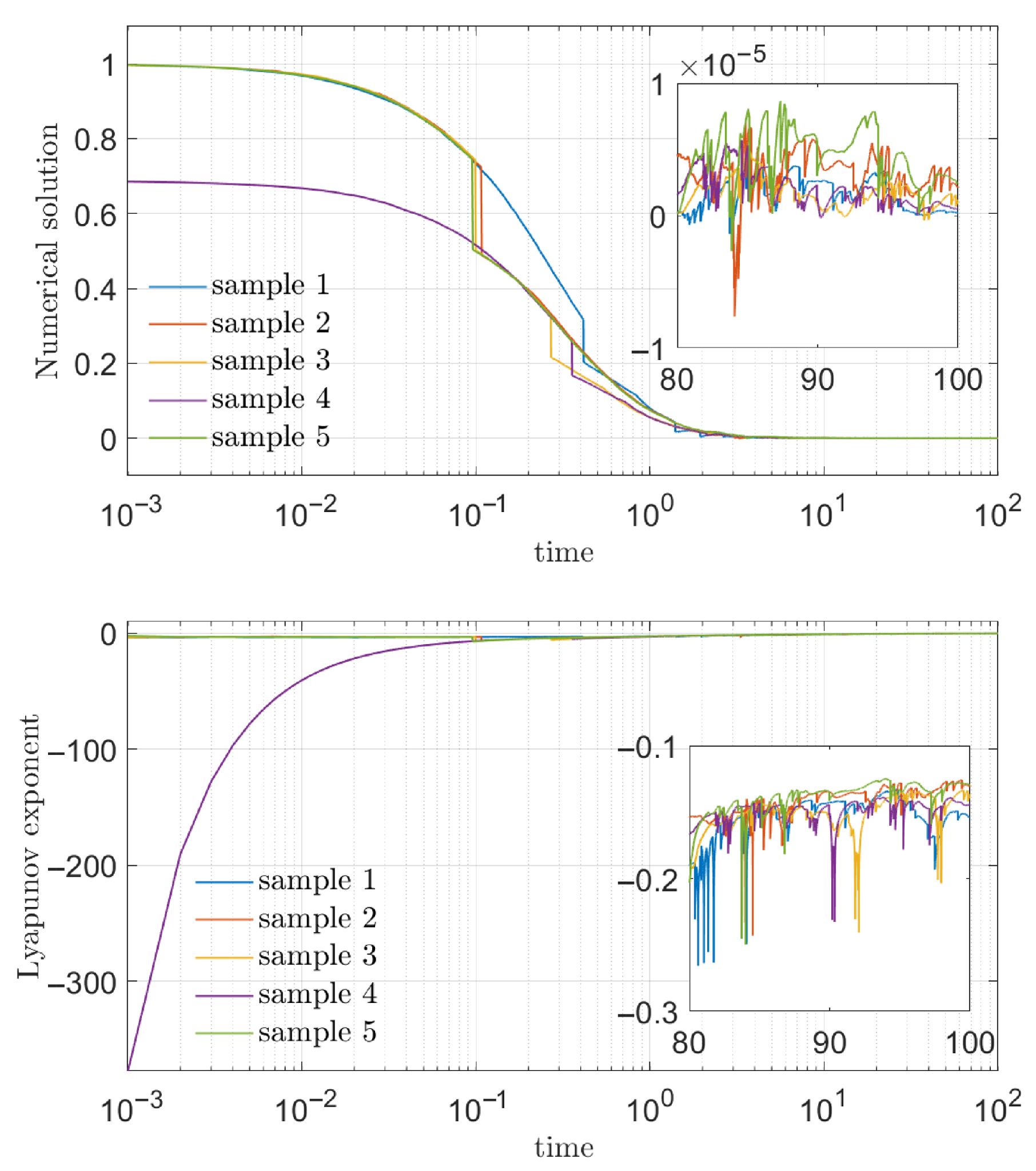
To validate these theoretical findings, we simulate the numerical solution of Equation (37) using the S S θ -method described in Equation (7), with initial conditions x 0 = 1 and r 0 = 1 . Following the simulation framework outlined in [33] (Chapter 4), the zero-one jump process is approximated via the acceptance-rejection method, under the assumption of a sufficiently small temporal step Δ . Here, we choose Δ = 0.001 and examine the method’s behavior for θ [ 0 , 1 ] in increments of 0.1 to comprehensively evaluate the performance of the S S θ -method. Additionally, to estimate the Lyapunov exponent numerically, we employ a Monte Carlo approach, generating 500 independent sample trajectories for each value of θ . Among them, five representative sample paths are randomly selected and used for visualization purposes. The Lyapunov exponents computed at final time T = 100 along these five individual sample paths are reported in Table 1.
The numerical solutions and Lyapunov exponents with respect to time over 500 discredited sample paths along 5 individual paths are shown in Figure 1 and Figure 2. By virtue of Figure 1 and Figure 2, it can be seen that the numerical scheme via the S S θ -method defined in Equation (7) is almost surely exponentially stable.

5. Conclusions

In this study, we propose a class of S S θ -methods for analyzing the stability of stochastic pantograph differential equations with Markovian switching and jump perturbations. While the literature has extensively addressed the stability of such systems, relatively few results are available concerning the stability properties of their numerical approximations. This work aims to bridge this gap by contributing new insights into the almost sure exponential stability concerning both the exact and numerical solutions. We first establish the almost sure exponential stability of the trivial solution to the underlying system. Under an additional assumption that the drift term satisfies a linear growth condition, we further demonstrate that the numerical solutions obtained using the proposed S S θ -method also retain this stability property. Finally, we support the theoretical analysis with numerical simulations, illustrating the effectiveness and consistency of the developed method.

Author Contributions

Conceptualization, G.L. and Z.H.; data curation, B.X. and Z.C.; formal analysis, G.L. and Z.H.; funding acquisition, G.L., Z.H. and F.D.; investigation, Z.H., B.X. and Z.C.; methodology, G.L. and Z.H.; project administration, F.D.; software, B.X. and Z.C.; supervision, F.D.; validation, B.X. and Z.C.; visualization, G.L. and Z.H.; Writing—original draft, G.L.; Writing—review and editing, Z.H. and F.D. All authors have read and agreed to the published version of the manuscript.

Funding

This research was partially supported by the National Natural Science Foundation of China (No. 11901398, No. 62473157, No. 62333006) and the Basic and Applied Basic Research of Guangzhou Basic Research Program (No. 202201010250).

Data Availability Statement

Data is contained within the article. The original contributions presented in this study are included in the article.

Conflicts of Interest

The authors declare no conflicts of interest.

References

  1. Appleby, J.A.D. Decay and growth rates of solutions of scalar stochastic delay differential equations with unbounded delay and state dependent noise. Stoch. Dyn. 2005, 5, 133–147. [Google Scholar] [CrossRef]
  2. Zhang, Y.; Zhang, E.; Li, L. The improved stability analysis of numerical method for stochastic delay differential equations. Mathematics 2022, 10, 3366. [Google Scholar] [CrossRef]
  3. Minhós, F.; Raza, A.; Shafique, U.; Mohsin, M. Modeling, analysis, and transmission dynamics of cassava mosaic disease through stochastic fractional delay differential equations. Mathematics 2025, 13, 383. [Google Scholar] [CrossRef]
  4. Jiang, F.; Shen, Y.; Liu, L. Taylor approximation of the solutions of stochastic differential delay equations with Poisson jump. Commun. Nonlinear Sci. Numer. Simulat. 2011, 16, 798–804. [Google Scholar] [CrossRef]
  5. Li, H.; Zhu, Q. The pth moment exponential stability and almost surely exponential stability of stochastic differential delay equations with Poisson jump. J. Math. Anal. Appl. 2019, 471, 197–210. [Google Scholar] [CrossRef]
  6. Kang, Y.H.; Jeong, J.M. Time-Optimal Control for Semilinear Stochastic Functional Differential Equations with Delays. Mathematics 2021, 9, 1956. [Google Scholar] [CrossRef]
  7. Mao, X.; Yuan, C. Stochastic Differential Equations with Markovian Switching; Imperial College Press: London, UK, 2006. [Google Scholar]
  8. Mao, X.; Matasov, A.; Piunovskiy, A.B. Stochastic differential delay equations with Markovian switching. Bernoulli 2000, 6, 73–90. [Google Scholar] [CrossRef]
  9. Song, R.; Zhu, Q. Stability of linear stochastic delay differential equations with infinite Markovian switchings. Int. J. Robust Nonlinear Control 2018, 28, 825–837. [Google Scholar] [CrossRef]
  10. Zhang, T.; Chen, H. The stability with a general decay of stochastic delay differential equations with Markovian switching. Appl. Math. Comput. 2019, 359, 294–307. [Google Scholar] [CrossRef]
  11. Wang, L.; Xue, H. Convergence of numerical solutions to stochastic differential delay equations with Poisson jump and Markovian switching. Appl. Math. Comput. 2007, 188, 1161–1172. [Google Scholar] [CrossRef]
  12. Zhang, W.; Ye, J.; Li, H. Stability with general decay rates of stochastic differential delay equations with Poisson jumps and Markovian switching. Statist Probab. Lett. 2014, 92, 1–11. [Google Scholar] [CrossRef]
  13. Ockendon, J.R.; Tayler, A.B. The dynamics of a current collection system for an electric locomotive. Proc. R. Soc. Lond Ser. A 1971, 322, 447–468. [Google Scholar]
  14. Zhang, H.; Xiao, Y.; Guo, F. Convergence and stability of a numerical method for nonlinear stochastic pantograph equations. J. Franklin Inst. 2014, 351, 3089–3103. [Google Scholar] [CrossRef]
  15. Fan, Z.; Liu, M.; Cao, W. Existence and uniqueness of the solutions and convergence of semi-implicit Euler methods for stochastic pantograph equations. J. Math. Anal. Appl. 2007, 325, 1142–1159. [Google Scholar] [CrossRef]
  16. Fan, Z.; Song, M.; Liu, M. The αth moment stability for the stochastic pantograph equation. J. Comput. Appl. Math. 2009, 233, 109–120. [Google Scholar] [CrossRef]
  17. Jiang, F.; Yang, H.; Wang, S. Asymptotic stability of stochastic pantograph differential equations with Markovian switching. J. Nonlinear Anal. Optim. 2010, 1, 9–16. [Google Scholar]
  18. Milošević, M. Existence, uniqueness, almost sure polynomial stability of solution to a class of highly nonlinear pantograph stochastic differential equations and the Euler-Maruyama approximation. Appl. Math. Comput. 2014, 237, 672–685. [Google Scholar] [CrossRef]
  19. You, S.; Mao, W.; Mao, X.; Hu, L. Analysis on exponential stability of hybrid pantograph stochastic differential equations with highly nonlinear coefficients. Appl. Math. Comput. 2015, 263, 73–83. [Google Scholar] [CrossRef]
  20. Mao, W.; Hu, L.; Mao, X. Almost sure stability with general decay rate of neutral stochastic pantograph equations with Markovian switching. Electron. J. Qual. Theory 2019, 52, 1–17. [Google Scholar] [CrossRef]
  21. Xiao, Y.; Zhang, H.Y. A note on convergence of semi-implicit Euler methods for stochastic pantograph equations. Comput. Math. Appl. 2019, 59, 1419–1424. [Google Scholar] [CrossRef]
  22. Baker, C.T.H.; Buckwar, E. Continuous θ-methods for the stochastic pantograph equation. Electron. Trans. Numer. Anal. 2000, 11, 131–151. [Google Scholar]
  23. Zhou, S.; Hu, Y. Numerical approximation for nonlinear stochastic pantograph equations with Markovian switching. Appl. Math. Comput. 2016, 286, 126–138. [Google Scholar] [CrossRef]
  24. Guo, P.; Li, C. Almost sure exponential stability of numerical solutions for stochastic pantograph differential equations. J. Math. Anal. Appl. 2018, 460, 411–424. [Google Scholar] [CrossRef]
  25. Cheng, M.; Zhang, W.; Li, R. Convergence and stability of the balanced Euler method for stochastic pantograph differential equations with Markovian switching. Int. J. Comput. Math. 2024, 101, 281–313. [Google Scholar] [CrossRef]
  26. Ding, X.; Ma, Q.; Zhang, L. Convergence and stability of the split-step theta-method for stochastic differential equations. Comput. Math. Appl. 2010, 60, 1310–1321. [Google Scholar] [CrossRef]
  27. Huang, C. Mean square stability and dissipativity of two classes of theta methods for systems of stochastic delay differential equations. J. Comput. Appl. Math. 2014, 259, 77–86. [Google Scholar] [CrossRef]
  28. Cao, W.; Hao, P.; Zhang, Z. Split-step θ-method for stochastic delay differential equations. Appl. Numer. Math. 2014, 76, 19–33. [Google Scholar]
  29. Mo, H.; Deng, F.; Zhang, C. Exponential stability of the split-step θ-method for neutral stochastic delay differential equations with jumps. Appl. Math. Comput. 2017, 315, 85–95. [Google Scholar] [CrossRef]
  30. Yuan, H.; Shen, J.; Song, C. Mean square stability and dissipativity of split-step theta method for nonlinear neutral stochastic delay differential equations with poisson jumps. J. Comput. Appl. Math. 2017, 35, 766–779. [Google Scholar]
  31. Xiao, Y.; Eissa, M.A.; Tian, B. Convergence and stability of split-step theta methods with variable step-size for stochastic pantograph differential equations. Int. J. Comput. Math. 2018, 95, 939–960. [Google Scholar] [CrossRef]
  32. Guo, P.; Li, C. Almost sure stability with general decay rate of exact and numerical solutions for stochastic pantograph differential equations. Numer. Algorithms 2019, 80, 1391–1411. [Google Scholar] [CrossRef]
  33. Hanson, F.B. Applied Stochastic Processes and Control for Jump-Diffusion; SIAM: Philadelphia, PA, USA, 2007. [Google Scholar]
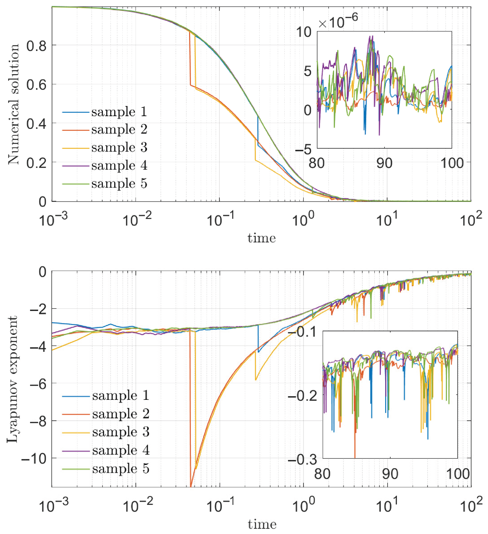
Figure 1. The numerical solution (up) and the Lyapunov exponent (down) of Equation (37) with θ = 0.4 and Δ = 0.001 over 500 discredited sample paths along 5 individual paths.
Axioms 14 00718 g001
Figure 2. The numerical solution (up) and the Lyapunov exponent (down) of Equation (37) with θ = 0.8 and Δ = 0.001 over 500 discredited sample paths along 5 individual paths.
Axioms 14 00718 g002
Table 1. Lyapunov exponents at T = 100 using SS θ -method in Equation (7) to Equation (37).
θ Sample 1Sample 2Sample 3Sample 4Sample 5
0.0−0.13672−0.13897−0.13034−0.18784−0.12176
0.1−0.12984−0.13489−0.12816−0.13406−0.12738
0.2−0.14278−0.14453−0.14883−0.15272−0.14469
0.3−0.1361−0.15363−0.16493−0.16144−0.1369
0.4−0.12721−0.13012−0.12988−0.12638−0.12565
0.5−0.13342−0.12176−0.12739−0.13461−0.14543
0.6−0.15233−0.13627−0.13078−0.14636−0.14031
0.7−0.12412−0.12947−0.1177−0.12865−0.12469
0.8−0.15403−0.13062−0.13635−0.14418−0.12927
0.9−0.12944−0.13174−0.12968−0.14019−0.13093
1.0−0.13241−0.12314−0.12265−0.12548−0.14104
Disclaimer/Publisher’s Note: The statements, opinions and data contained in all publications are solely those of the individual author(s) and contributor(s) and not of MDPI and/or the editor(s). MDPI and/or the editor(s) disclaim responsibility for any injury to people or property resulting from any ideas, methods, instructions or products referred to in the content.