1. Introduction
Queuing theory plays an important role in decision making by providing insight into the operation and efficiency of queuing systems. It deals with the mathematical modeling of customer arrivals and the corresponding service times in queuing systems. A key aspect of queuing theory is decision optimization, which focuses on examining the underlying parameters and constraints of a model and helps decision makers optimize performance measures. Various queue configurations can be analyzed, such as the speed of service and number of servers, to assess the most cost-effective and efficient strategy.
Another aspect of queuing theory in the context of decision making is sensitivity analysis. It allows decision-makers to analyze various scenarios by modeling several queue configurations and to identify the impact of variations in system parameters, particularly the cost of changes in customer service models. In addition, it allows decision makers to realize the possible consequences of different system parameters and to take informed action by understanding system dynamics (see [
1]).
Queues are used in a variety contexts, such as mobile data in the wireless mobile systems discussed by Li et al. [
2] and patient flow in the clinics studied by Aziati and Hamdan [
3], etc.
Reducing customer congestion in any service system is a common problem, and it is the main challenge in queue management. Its importance is highlighted in a variety of ways in numerous research studies, such as, for example, the loss of productivity that occurs due to time lost in traffic (De and Rajbongshi [
4]), health impacts (Requia et al. [
5]), etc.
To solve the problem of reducing customer congestion in queues, increasing the number of servers assigned to a system is an immediate solution, but adding each server incurs service costs. This challenge has been taken up by many researchers in order to determine the optimal number of servers while considering the cost function as an objective, as explained by Lefebvre and Yaghoubi [
6]. Consequently, a compromise must be found between customer congestion and the total cost of a faster service, either through the speed of service or the number of servers. Therefore, characterizing the optimal-service rate in a system is a fundamental factor in practice for how operations should be conducted.
Many papers have investigated variations in the service rate to reduce queues. In the age of artificial intelligence, a wide range of optimization techniques based on computational methods have been introduced, as shown by Laxmi and Jyothsna [
7]. The aforementioned authors examined a discrete-time queue using particle swarm optimization to optimize service rates in order to minimize costs, and their paper explored its application in inbound email contact centers.
New mathematical programming models are recent directions of the research in this area, such as Tian et al. [
8]. These authors studied a single-server queuing system with varying service rates to analyze how customer decisions affect the equilibrium performance of a queue using continuous-time Markov chains for modeling and analysis. Singh et al. [
9] investigated a method for detecting change points in the service rate of an
queue by analyzing the changes in the probability distribution of a stochastic process using a likelihood function based on the number of customers observed at departures and via employing Bayesian estimators.
Laxmi et al. [
10] proposed an
queuing system with an alternative second service using a system stabilization and performance evaluation method. Wu et al. [
11] examined a queuing system that could be used to control customer arrivals, as well as a
queue with variable service speeds. They performed a steady-state analysis for system optimization, with the objective of reducing costs and waiting times. The results show a diminishing return on additional investment in efficient systems, and regression models are proposed for decision making. Chen et al. [
12] studied service rate control using event-based optimization to obtain optimal control policies. They proposed an algorithm for determining service rates and compared its effectiveness with state-based optimization.
Dudin et al. [
13] analyzed a queuing system with two different types of requests: Type 1, i.e., with a constant service rate; and Type 2, i.e., with flexible rates. They explored the behavior of the system through a Markov chain, focusing on performance measures and the optimal service assigned for the two types of requests. Lakkumikanthan and Balasubramanian [
14] developed an optimal service rate decision for a discrete-time queuing system with a finite buffer employing Markov decision theory and linear programming. The aim was to optimize costs by regulating service rates based on customer arrival and inventory reloading. Su and Li [
15] focused on a single-server queue in communication networks with varying service rates and various types of customers. Their paper compared control levels based on various parameters and chose an optimal policy when multiple optimal policies were available. Büke and Qin [
16] studied multi-server queuing systems with varying rates of service using stochastic processes to analyze performance. They used martingales to characterize these processes under different policies.
For an overview of other studies in this area, the reader is referred to Dai et al. [
17], Chen and Xia [
18], and Rodrigues et al. [
19].
In this paper, we suppose that the random service time is either
or
. Moreover, in
Section 2, the server can switch between
and
at any time instant.
2. Problem Description
We denote respectively by and the total number of customers in the system and the number of customers who are waiting in line at time t. We suppose that at the initial time , , where is the capacity of the system, which can be infinite. The server therefore starts his/her service at time , which could be, for example, the opening time of a shop.
We define the
first-passage time as follows:
Our aim is to determine whether the server should choose the service time
or
at time
t to minimize the expected value of the criterion function:
where
or
,
and
are positive constants, and
is the terminal cost function. If
, then the instantaneous (or running) cost
will be smaller. However, it will take longer to reduce the number of waiting customers to zero, thus incurring a larger penalty (since
). The optimizer must also take into account the terminal cost
.
Remark 1. The term in the cost function corresponds to in LQ or LQG optimal control problems. Moreover, when does not depend on t and , as will be the case in Section 4, if we use in the cost function, then cancels out, so that the expected service time is not taken into account. The optimal control problem considered is a particular
homing problem (see Whittle [
20]). In these problems, the optimizer tries to find the control of a stochastic process that minimizes the expected value of a given cost function between an initial time and the time when a certain event occurs. Whittle [
20] treated the case when the stochastic process is an
n-dimensional diffusion process. Rishel [
21] set up such problems for
n-dimensional diffusion processes that can be used to model the wear of devices. Lefebvre has written numerous papers on homing problems. In a recent one ([
22]), he extended homing problems to the case of autoregressive processes (see also Lefebvre and Pazhoheshfar [
23] for an optimal maintenance problem).
Homing problems for modified
queuing systems were treated by Lefebvre in [
24,
25], and by Lefebvre and Yaghoubi [
6]. In these papers, the control variable was the number of servers working at time
t.
Remark 2. There are numerous applications of queuing theory. In many situations, time is indeed a random variable. For example, suppose that the “customers” in the systems are orders received by a company. The time required to fill the orders is generally not fixed. Moreover, the constant could be the deadline by which orders are fulfilled, where otherwise a penalty is imposed on the company.
In
Section 3, we will present an aeronautical application. In this case, the customers are aircraft that have been brought to a workshop for maintenance. The aim, of course, is to get the aircraft back into service as quickly as possible. Once again, the time required to carry out maintenance is random since problems may be detected during the basic inspection.
Next, we define the
value functionThat is,
is the expected cost incurred if the optimizer chooses the optimal control between the initial time
and the random final time
. Moreover, we assume that
where
. It then follows that the value function satisfies the boundary conditions
Remark 3. The aim is to empty the queue at the latest by time , which is a fixed constant. If we had not succeeded in doing so by time , we stop the optimization problem and a cost is incurred.
In
Section 3, we will use the fact that, when
Exp
, that is, when
has an exponential distribution with parameter
for
, it is possible to make use of dynamic programming to determine the optimal control. In the general case, assuming that the optimizer chooses either
or
for all
t in
, we will use conditional probability to find the optimal solution. This will be conducted in
Section 4. Finally, we will conclude with a few remarks in
Section 5.
3. Optimal Control of the Modified Queue
When
Exp
, we have a modified
queuing model, in which the service time distribution is not fixed. We can then write the cost function
as follows:
where
or
.
Let
A be the time needed for a new customer to arrive after time
. We have
Exp
, so that
and, similarly,
Furthermore, the probability of two or more events (arrivals or departures) in an interval of length is equal to .
Since, by independence,
Exp
, the random number
of customers in the system at time
will be
Next, with the help of Bellman’s principle of optimality, we may write that
We then obtain, through writing
,
Furthermore, using Taylor’s formula, we can write that
Hence, through also applying Taylor’s formula to the terms
and
, we obtain that
Finally, via dividing both sides of the previous equation by and letting decrease to zero, we obtain the following proposition:
Proposition 1. If Exp, for , the value function satisfies the following dynamic programming equation (DPE): Moreover, we have the boundary conditions in Equation (5). Remark 4. Equation (15) is valid for any if the capacity of the system is infinite. In the case when , Equation (9) for reduces to It follows that the dynamic programming equation becomesfor . We could also assume, for instance, that if a customer arrives while the system is already full, then we stop the control problem and we set . We would then havefor . In this paper, we assume that Equation (17) is the one that is valid if . Next, since
or
, Equation (
15) can be rewritten as follows:
To determine the value of
, we can first consider the differential equation deduced from Equation (
19) if the optimizer chooses
for any value of
k and any
, namely
which is subject to the conditions in Equation (
5). To obtain
, we must, in general, solve a system of first-order linear differential equations.
Once the functions
have been computed for
and for any
k, we define it as follows:
for
. The function
is the right-hand side of Equation (
15) if
. We can determine the optimal control by comparing the two functions for any
.
Finally, to obtain the value function
, we can solve the equation
in any interval where the optimal control is
, and we can make use of the boundary condition
, as well as the continuity of the function
.
Remark 5. It is important to note that dynamic programming only works for the model (apart from a few special cases considered in other recent papers by the first author). Indeed, the results given in Equations (7) and (8) do not hold for general distributions. If or is not proportional to , there will be a problem when we divide both sides of Equation (14) by and we let decrease to zero. Assuming that A and are exponentially distributed is a simplifying assumption. Nevertheless, we believe that the model can serve as an approximate model in various applications. We will now give an example that can be solved explicitly.
An Example
The simplest problem that can be considered is the one when
. We then have the following equation (see Equation (
17)):
The solution that satisfies the boundary condition
is
Let us take
,
,
,
,
and
. We then have
and
for
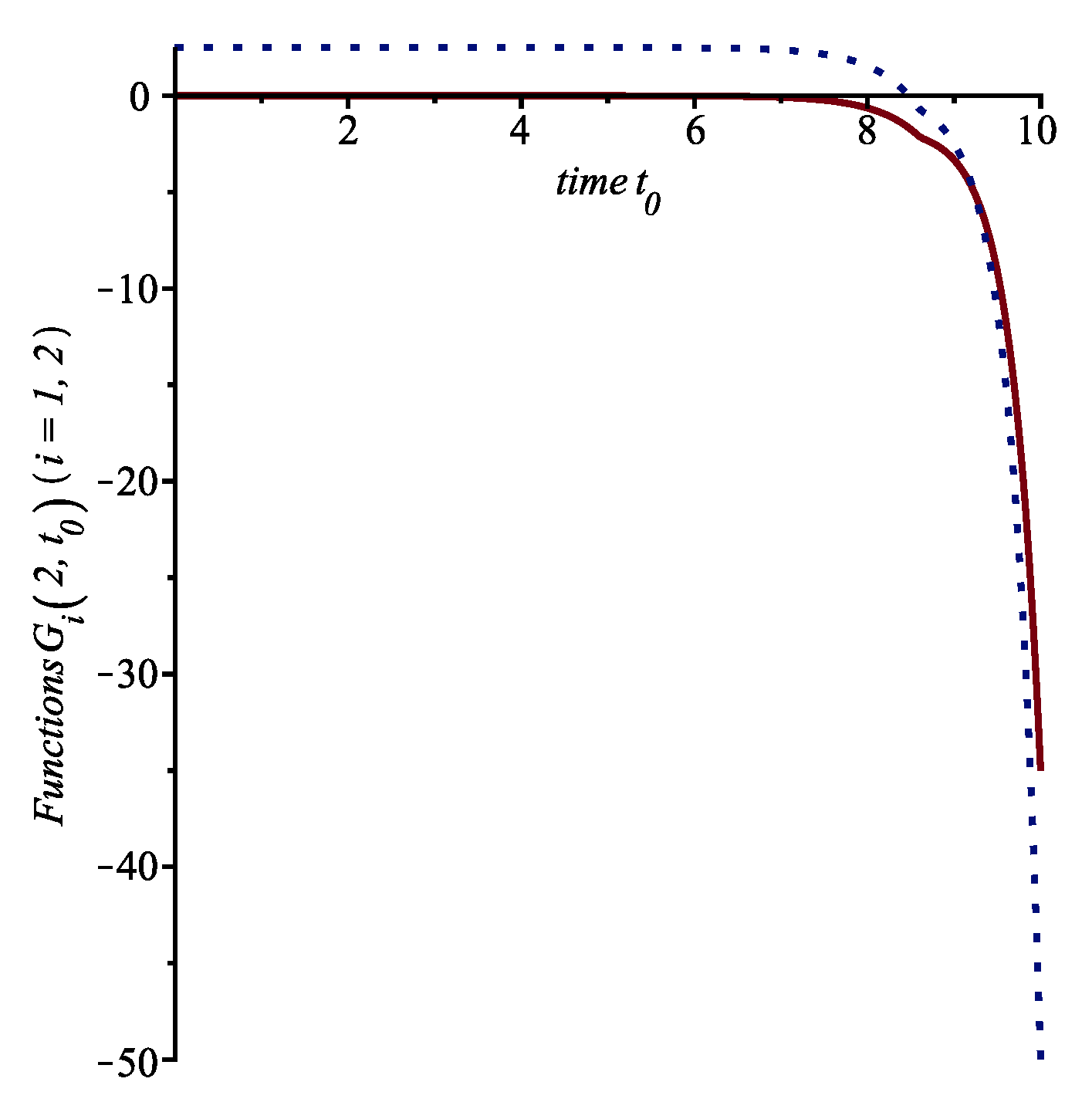
. We can now compute the functions
and
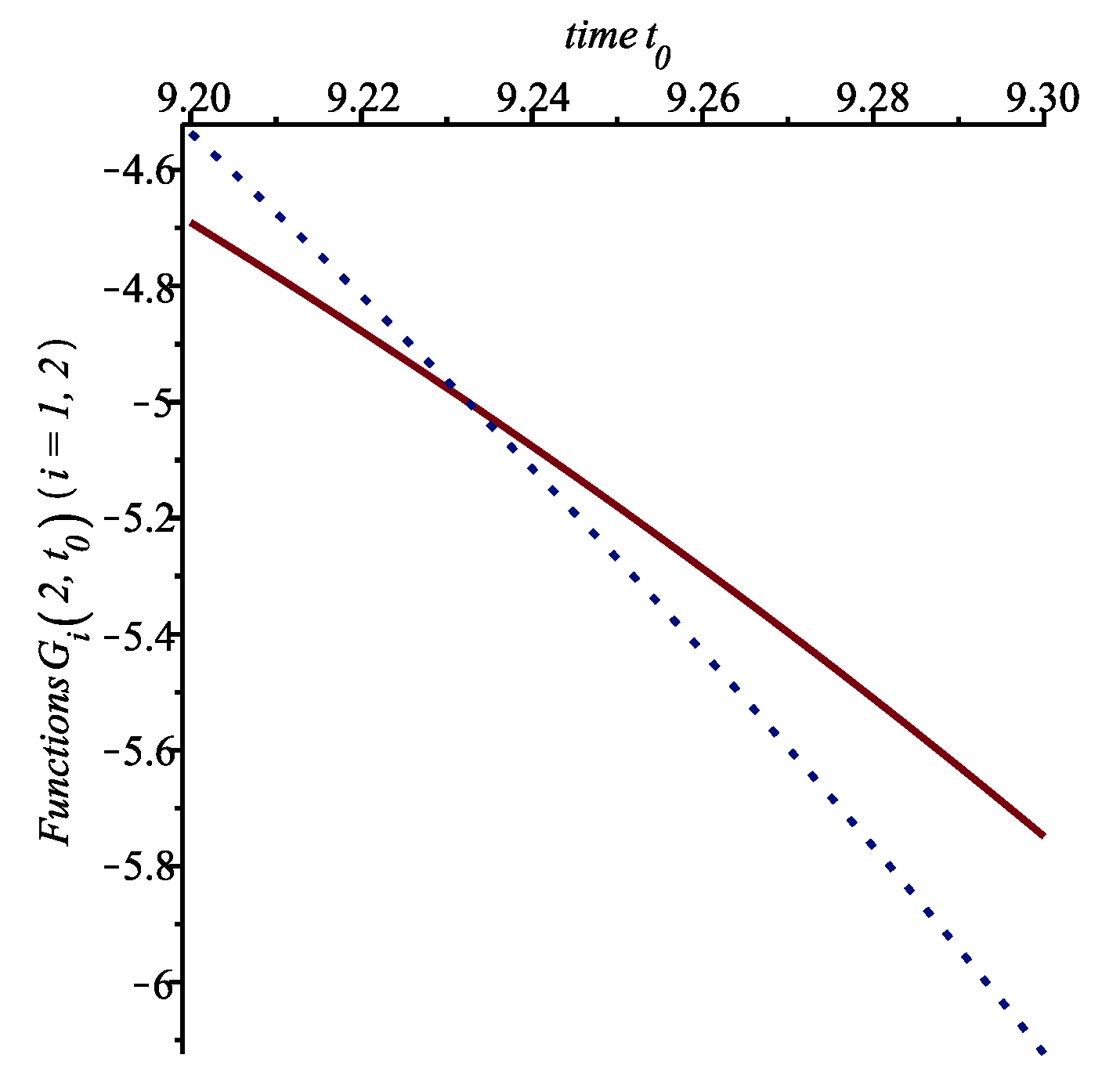
. These functions are displayed in
Figure 1 and
Figure 2. The curves cross when
. It follows that we then can write that the optimal control is
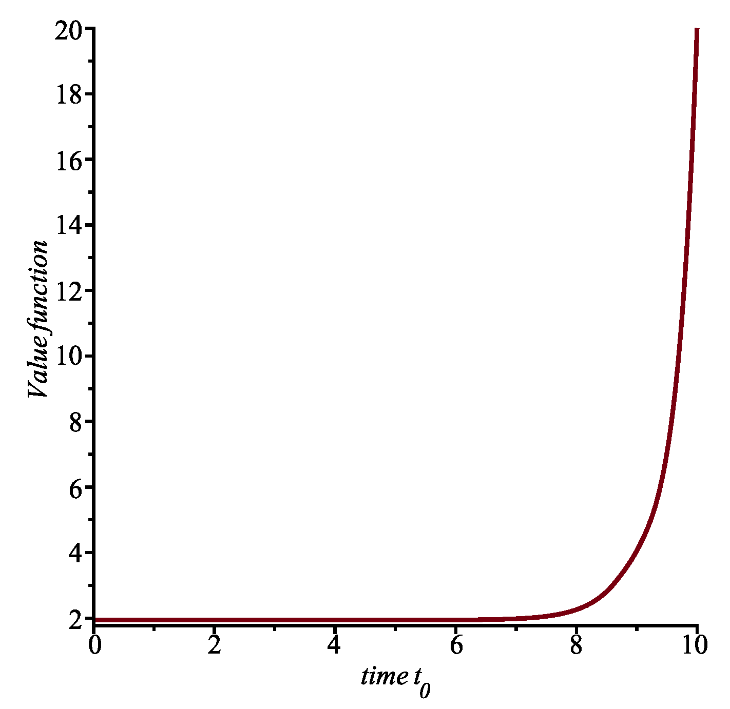
Finally, proceeding as explained above, we can calculate the value function
, as shown in
Figure 3.
In the next section, we will consider the case when the service time distributions are not necessarily exponential.
4. Optimal Control of the Modified Queue
Suppose that the optimizer must choose either the random service time
or
from the initial time
to the final time
and that the function
is identical to zero, so that the expected value of the cost function
defined in Equation (
2) becomes (setting
equal to zero)
where
or
. We will consider various particular cases below.
Case 1. Assume that
. Since it is full, no new customers can enter the system between
and
. Moreover, we can write that
is simply equal to
S. Thus, it follows that
In the special case when
Exp
, for
, the above equation becomes
so that
Suppose that , and . Then, we find that the optimal solution is if and only if .
Remark 6. If we take the limit as tends to infinity in Equation (24), we obtainwhich agrees with Equation (31) above. Case 2. Let
and
. We can write that
where
is the time needed to serve the first customer, and
Exp
is the time between successive customers, which is assumed to be independent of the service times. It then follows that
If
Exp
, we have
Thus,
To obtain the optimal solution, we must compare the value of
deduced from Equation (
28) and the above formula when
with the corresponding one when
.
Remark 7. Let be independent random variables that have an Exp distribution, and let N be a geometric random variable with parameter Hence, we retrieve the formula in Equation (36). For the next cases, we will denote by .
Case 3. When
and
, no new customers can enter the system during the service time of the first customer. Hence, we can write that
When
Exp
, we obtain that
Remark 8. In Section 2, to obtain the function , when , we must solve the system of first-order linear differential equations The solution to this system that satisfies the conditions in Equation (5) is easy to obtain. If we set and , we find that the limit as tends to infinity of the solution is given by Notice that and (see, respectively, Equations (36) and (40)). Case 4. Finally, suppose that
and
or
. We then define the event
as follows: there are exactly
i customers that arrive during the service time
of the first customer, for
, and we denote by
(respectively,
) the time needed for the first (and, respectively, second) new customer to arrive during the service time
. We can thus write that
To obtain and , we can solve the above system of two linear equations. The various probabilities that appear in the system can at least be evaluated numerically in any particular case.
4.1. Particular Problem
We consider a particular problem in Case 4. Suppose that
Exp
and
G
, that is,
has a gamma distribution with both parameters equal to 2, so that
Notice that . It then follows that the optimal control will depend only on the value of for and .
Let
and
where
is the random variable
if
for
. We then find that
Notice that for , as required.
Let
be the value of
if
, for
. To obtain
and
, we must solve the following system of linear equations:
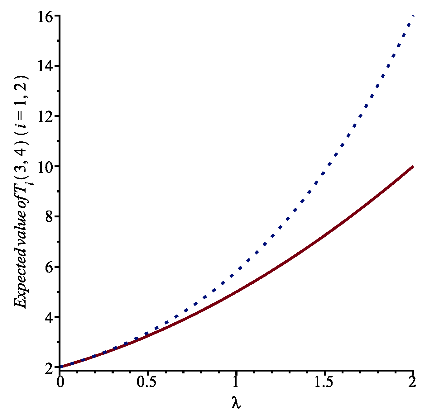
We can see that and are almost equal when is very small. However, as increases, is much smaller than . In actuality, we can show that for any . Hence, the optimal solution is always to choose . The same conclusions apply to and .
4.2. A Practical Application
We consider the problem of selecting an optimal-control policy for aircraft maintenance. In practice, maintenance programs must be optimized to minimize downtime and guarantee the expected level of safety, which are two fundamental elements in the aerospace industry. In our problem formulation, we must balance maintenance costs and the need to return the aircraft to service as soon as possible.
Suppose that
is a Rayleigh random variable, so that
where
is a positive constant and that
That is, is an exponential random variable with parameter . The Rayleigh distribution, with its longer tail, should be more appropriate in the case of complex maintenance activities, while the exponential distribution could be used for customary maintenance activities.
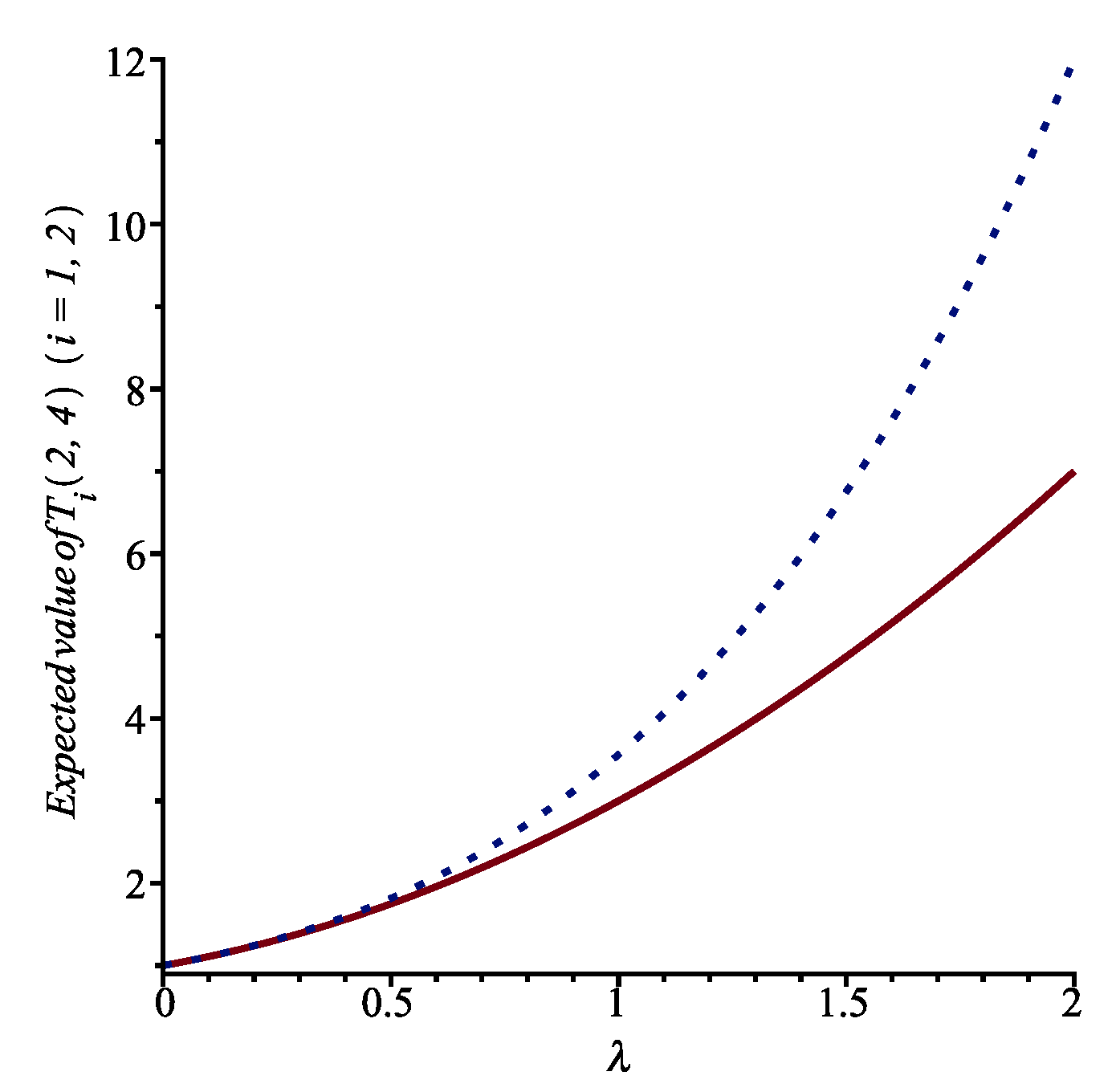
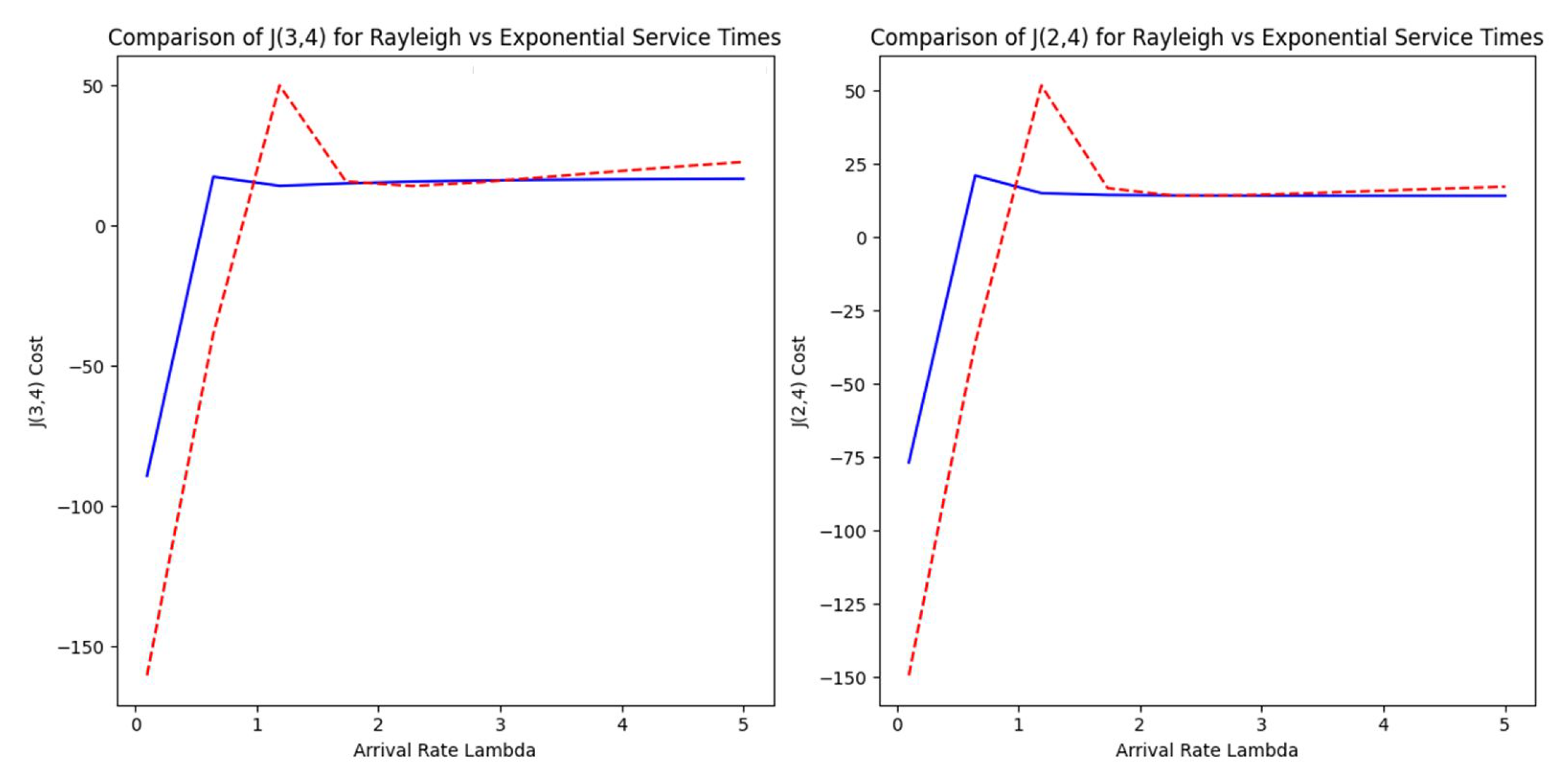
The expected costs and for performing the maintenance tasks under each of the two different service time assumptions for a variable aircraft arrival rate for service were calculated. These costs include costs related to the speed of task execution (influenced by the service time distribution) and costs related to aircraft downtime (influenced by ).
In
Figure 6, we present the expected costs
and
when
,
,
and
. Looking at the figure, we can conclude that, for routine inspections and predictable maintenance activities, the use of exponential service time distribution would be more cost effective, especially when arrival rates are high and rapid changes are required.
For more complex activities that vary significantly over time (potentially due to unexpected complexities during the maintenance tasks), a more realistic modeling policy is offered by the Rayleigh distribution, although it may induce a higher cost. Such information would be essential for efficient planning and resource allocation, particularly in ensuring the availability of adequate maintenance personnel and spare parts.
Maintenance centers and airlines may decide to modify the planning of their maintenance decisions according to the historical frequency of maintenance needs (reflected by ) and the complexity of tasks (complex or normal). For example, during busy seasons, it may be more cost effective to give priority to minimizing downtime (by choosing the exponential distribution).
5. Conclusions
We treated an optimal control problem for a queueing model with only one server. This queueing model was a modification of the classic model, in which the server can now choose between two distributions for the service time. The aim was to reduce the waiting queue to zero as soon as possible, while taking the quadratic control costs into account. The final time in the problem is the first time nobody is waiting for service in the system.
In
Section 3, we assumed that the service time was exponentially distributed, with parameter
or
. We could then make use of dynamic programming to derive the equation satisfied by the value function, which gives the expected cost if the optimizer uses the optimal control from the initial time to the random final time.
Next, in
Section 4 we generalized the problem to the case when the service time is any positive random variable. In general, it is then not possible to appeal to dynamic programming. We considered various particular cases when the capacity of the system is finite. We could in theory try to solve any particular problem. However, if the capacity of the system is large, the technique used to find the optimal solution will become rather intricate.
It is of course possible to consider other modifications of the basic queue. We could also assume that there is more than one server. The aim could be to use some control in order to increase the rate at which customers enter the system. If all the random variables in the model are exponentially distributed, we could try to utilize dynamic programming principles to obtain the optimal solution.
