Abstract
This paper investigates a quantum system described by the Schrödinger equation, utilizing the concept of the quantum Lyapunov function. The Lyapunov function is chosen based on the mean value of a virtual mechanical quantity, where different values of P, the mean value of the virtual mechanical quantity in the Lyapunov function, have an impact on the attractive domain of the quantum system. The selected primary optimization algorithms approximating matrix P are the particle swarm optimization (PSO) algorithm and the simulated annealing (SA) algorithm. This study examines the characteristics of the system’s attraction domain under these two distinct algorithms and establishes stability conditions for the nonlinear quantum system. We introduce a method to estimate the size of the attractive domain using the Lyapunov function approach, converting the attractive domain issue into an optimization challenge. Numerical simulations are conducted in various two-dimensional test systems and spin 1/2 particle systems.
Keywords:
Schrödinger equation; nonlinear systems; Hermitian operator; attraction domain; optimization MSC:
34A05; 37A55; 49N05; 81P50
1. Introduction
For a quantum system described by the Schrödinger equation, stability analysis and controller design are fundamental tasks. The Lyapunov method is popular in the dynamic system analysis and control coupling, which also plays a significant role in quantum control research. This method ensures that the designed control laws do not cause the closed-loop system to diverge. A key challenge lies in selecting an appropriate Lyapunov function, as different functions yield varying control laws and effects. This paper selects a Lyapunov function based on the mean value of virtual mechanical quantities. In quantum theory, the Hermitian operator P represents a system’s mechanical quantity. If the system is in P’s eigenstate, then P’s mean value is its corresponding eigenvalue. By using this Lyapunov function, the proposed feedback control law can locally asymptotically stabilize quantum systems in any desired Hamiltonian eigenstate. The choice of P affects the target eigenstate’s attractive domain size. This paper primarily investigates how specific P choices enlarge the target eigenstate’s attractive region and system’s local asymptotic stability region. A nonlinear system attraction domain analysis focuses on closed quantum systems described by the Schrödinger equation, where control strength tends to be represented by the wave function, rendering the system nonlinear. The concept of quantum Lyapunov control involves designing a control law that ensures the Lyapunov function’s time derivative remains non-positive. In experiments, control intensity is typically managed via laser intensity selection. Various Lyapunov control methods have been developed for control law design [1,2,3,4,5,6,7,8].
The quantum system described by the Schrödinger equation presents interesting challenges in stability analysis and attraction domain estimation. The pioneering research on this topic dates back to the 1960s when Zubov [9] introduced the concept of the asymptotically stable region, effectively estimating the system’s attraction domain. Following Zubov’s work, Davison and Kurak [10] in 1971 approached the attraction domain as a hyperplane for estimation purposes. Later, Blankenship and Loparo [11] employed linearization techniques to study the attraction domain of analytic polynomial systems within a specific subset.
In the 1980s, Thorp [12] introduced a novel algorithm for estimating the attraction domain of nonlinear systems, demonstrating its applicability to high-dimensional systems as well. Khalil [13] further summarized advancements in estimating attraction domains for nonlinear systems during the 1990s. Subsequently, numerous constructive methodologies have been developed to address this estimation challenge, enriching the field significantly [14,15,16].
Notably, Hahn reframed the attraction domain estimation issue as an optimization problem, offering a fresh perspective. This shift led to increased interest in optimization-based estimation methods. Vannelli [17], for instance, introduced the concept of the maximum Lyapunov function, selected a rational Lyapunov function, and applied Taylor expansion to impose additional constraints on the optimization problem, thereby potentially expanding the attraction domain. To date, researchers across various disciplines have delved into the complexities of attraction domain problems, contributing a wealth of knowledge to this specialized field [18,19,20,21,22,23,24].
In this paper, the Lyapunov function based on the mean value of the virtual mechanical quantity is investigated. Two algorithms for calculating the mean value of the virtual mechanical quantity P, namely particle swarm optimization and simulated annealing, influence the size of the system’s attractive domain. The focus of this study is to estimate the attraction domain of the target eigenstate under varying P values. By analyzing these estimated attraction domains, we can evaluate the impact of different algorithms and establish a criterion for selecting algorithms when addressing the matrix P. This constitutes the primary contribution of this research. To tackle the attractor domain estimation challenge, the Lyapunov function method is employed, transforming the problem into an optimization task. Numerical examples reveal patterns in the P values determined by diverse algorithms.
The remainder of this paper is structured as follows: Section 2 provides the preliminary knowledge, defining Lyapunov function stability and the concept of the attraction domain. In Section 3, we describe the system under investigation. Section 4 delineates the stability conditions for nonlinear systems and estimates the attraction domain based on an optimization problem. This estimation problem is reformulated into an optimization problem, with a specific algorithm provided. Section 5 presents additional numerical examples to validate our findings. By utilizing different P values derived from the PSO algorithm and the simulated annealing algorithm in [8], we perform the attraction domain estimation using the optimization method developed in this paper. Finally, Section 6 summarizes the paper.
2. Preliminaries
2.1. Lyapunov Stability
The following nonlinear systems are mainly studied in this paper:
where and the function satisfies the local Lipschitz condition.
Definition 1.
If , the point is called the equilibrium point of system (1), and if , , , is called the isolated point of the system.
Definition 2.
Let be a continuous differentiable function defined by D; if it is satisfied, then the following is obtained:
- (i)
- is a positive definite on D;
- (ii)
- is negative on D, and then is called a Lyapunov function of the system.
Definition 3.
Let be the solution of system (1) with initial time and initial point ; for , if , when , such that
then, system (1) is stable.
Definition 4.
The origin of system (1) is satisfied
- (i)
- The origin is stable;
- (ii)
- , when , .
Then, system (1) is asymptotically stable.
Remark 1.
It is often convenient to “shift” the equilibrium to the origin before analyzing the characteristics of the system near the origin by means of coordinate transformations, so we only analyze the stability of system (1) at the origin.
Definition 5.
A square matrix F is defined; if all its eigenvalues have negative real parts, the matrix is called a Hurwitz matrix.
Theorem 1
([25]). Let :
- (i)
- If all eigenvalues of G have negative real parts, system (1) is asymptotically stable.
- (ii)
- If one or more eigenvalues of G have positive real parts, the origin is unstable.
Theorem 2
([26]). Let be a Lyapunov function of system (1) in the region
where . If is negative definite on , the origin is asymptotically stable, and when , each solution on tends to the origin.
2.2. The Definition of Attraction Domain
The attraction domain of system (1) is defined as follows:
where represents the solution of system (1), and the initial point is .
Remark 2.
All the aforementioned definitions and theorems are referenced in [13].
2.3. Problem Formulation for the Attraction Domain Estimation Based on Optimization
2.3.1. Formulation of an Optimization Problem
Consider the Lyapunov function and the hyperplane, which is given by
The negative region of is defined as , and the attraction domain is contained in the region .
If the maximum value of in can be found such that the is completely contained in the region of , the elliptical region will be the maximum approximation of the attraction domain of system (1). This observation and idea lead the formulation of an optimization problem in the following:
In this way, the problem is transformed as the problem of finding the minimum value of the Lyapunov function in the hyperplane (2).
2.3.2. Specific Algorithms
Write the attraction domain as
then, we have
.
In this way, the optimization problem (3) can be transformed into
where . The estimation of the attraction domain for system (1) can be approximated by solving the optimization on any mathematical software packages.
3. Quantum System Described by the Schrödinger Equation
Consider the quantum system described by the Schrödinger equation:
where j is the imaginary unit, is the internal Hamiltonian of system (5), is the control Hamiltonian related to the outside, and is the input control field. can be expressed as , and are the eigenvalues of corresponding to the eigenvector in . is an input control law that plays a role of normative freedom and it can be used to adjust the global phase without changing the system distribution. and are independent to each other.
For system (5), it is assumed that the target state satisfies the condition , and is the eigenvalue of the corresponding target state. If is selected, then it leads to . In order to facilitate the stability analysis of system (5), we choose the real number space to describe the system of Equation (5) in this paper, and we also need to separate the real part and imaginary part of the coefficient matrix in Equation (5) by virtue of the quantum state. Let the controlled state , and the real part and imaginary part on both sides of Equation (5) be equal, respectively, then the following state corresponding to the real vector x is obtained:
where , , represents the imaginary part, represents the real part, and A and satisfy , . From the above transformation, the dimension of vector x in the real-state space becomes .
In [8], we study the Lyapunov function in three forms, in which the Lyapunov function based on the mean value of virtual mechanical quantities is expressed as
The Hermitian operator P represents a mechanical quantity within a quantum system. Typically, the mean value of P, which pertains to virtual mechanical quantities in the Lyapunov function, necessitates estimation. Paper [8] discusses the particle swarm optimization (PSO) algorithm and the simulated annealing algorithm, both of which are prevalent methods that are particularly adept at solving for the P-value. Once the value of P is ascertained, the Lyapunov function V can be derived from Equation (7). However, varying P-values influence the estimation of the attraction domain for system (5), with the size of this domain indicating the region of the system that exhibits local asymptotic stability. Consequently, comparing the sizes of the estimated attraction domains under different P-values, as determined by distinct algorithms, emerges as an intriguing issue. Such comparisons offer a benchmark for assessing the impact of various algorithms on P.
4. Stability Analysis and Attraction Domain Estimation of the Quantum System
In this section, the stability analysis of the quantum system (5) is investigated, the attraction domain of system (5) is estimated by the optimization method (3) and (4). Different effects of the P-value in the Lyapunov function on the attraction domain of the quantum are also studied.
4.1. Stability Analysis of the Quantum System
Firstly, we consider the linear system
and its nonlinear perturbation system
where is a smooth vector field function defined on and the state . For the above systems, a theorem about the stability of perturbated systems is given in [27].
Theorem 3
([27]). If system (8) is asymptotically stable, and the nonlinear perturbation of system (9) satisfies when , then the zero solution of system (9) is locally asymptotically stable.
Remark 3.
We omit the proof of Theorem 3 here, but detailed proof can be found in [27]. Theorem 3 shows that for nonlinear perturbations, the stability of the linear part can guarantee the corresponding local stability of the nonlinear system.
Write system (9) as follows:
where x is the state of the system and is the Hurwitz matrix; Equation (10) can be obtained by the Taylor expansion.
Lemma 1
([28]). If is a Hurwitz matrix, assume that the Lyapunov function , where , and ; if , then system (10) is asymptotically stable.
Proof.
The derivative of is . Take ; then, . When and , then , and the equilibrium state of system (10) is asymptotically stable. □
The following is how to find a linear feedback that makes the system asymptotically stable. The attraction domain of a dynamic system is related to the stability of the system, i.e., the system must be asymptotically stable. In this section, we will investigate the stability of the nonlinear system in the case of Equation (6) for , and the same method works for the case of any i. Firstly, we study the stability condition corresponding to .
Consider the nonlinear system
It is assumed that u is a single input and a smooth linear feedback in (11). Let . For system (8) with equilibrium point , the stabilization problem is to find a smooth state feedback with , and , so that the closed-loop system is asymptotically stable with feedback .
Consider the linear system (11) with the single control input
where . Assuming that is a control pair, that is, satisfies the controllable condition , where , the linear performance controllability of system (12) is a sufficient condition to ensure that there is a local stable feedback control at the origin of system (11). In the case of (12), where is controllable and u is a single input, and , where . Based on the above conclusions, Equation (11) can be converted into the following form:
The first term on the right side is the linear part of the system if the eigenvalue is the linear part of the system, i.e., the eigenvalue of . If it is located in the left half of the complex plane, then (12) is asymptotically stable. For the nonlinear term , take the Lyapunov function ; and from the Lemma 1, it can be seen that when , the system is asymptotically stable, and also the estimation of the attraction domain can be performed.
How to choose K is also a problem to be solved, which should be selected according to the specific form of the system, and when the system is linear, K is selected to satisfy that the eigenvalue of the system is in the left-half plane of the complex plane. For the nonlinear term K, take the Lyapunov function , and it must satisfy . There is no unique way to take K, and it is sufficient to meet the asymptotically stable conditions. For the Lyapunov function , P satisfies .
4.2. Attraction Domain Estimation
For the closed quantum system (12) with the obtained input control law, the attraction domain plays an important role in the system dynamic analysis and the performance of the input feedback control law. With the optimization method (4), we can estimate the attraction domain of the closed quantum system. For the case of single input and , the following is an example to show how to estimate the attraction domain for the closed quantum system. For the case of , it is studied in Section 4.3.
Consider the case of in system (5); let the , , , and in the following, we estimate the attraction domain by solving the optimization problems (3) and (4).
The , of the above system are converted into the form of Equation (5), and then
Choose the Lyapunov function . According to , . The nonlinear term , . From Lemma 1, for the asymptotical stability of the closed quantum system, it must satisfy , and then K can be taken as , which makes the above conditions to be satisfied.
Substituting the above-obtained K into system (11), the selected Lyapunov function is . The derivative of is
The optimization problem (3) can be written as follows:
According to (4), the optimization problem can be transformed into
where . Here, we choose , , solved by Matlab, .
4.3. Attraction Domain Estimation with Two Different P-Values
In [8], we have studied a feedback control law for a special case of Equation (5) when :
As we have discussed in Section 4.1, the Lyapunov method is a popular method for the dynamic analysis of the quantum system. There are different Lyapunov function candidates for the quantum system, among which the Lyapunov function based on the average value of virtual mechanical quantities is expressed as in (7).
The first derivative of the Lyapunov function V with respect to time is
where [.,.] denotes the switcher of two matrices, such as . A, B is the Hermitian operator. Because , transposers are not determined by signs. For the convenience of the construction of P, the following can be made: . Write , ; then, the derivative of V with respect to time can be rewritten as
The control law we choose is and can take any value, which can guarantee that is less than or equal to zero [29,30]. The specific selection method of the control law here is consistent with that in [8].
With the method for in Section 4.2 and the obtained feedback control law, stability analysis and attraction domain estimation can also be investigated. In [8], we show that the system is asymptotically stable under this control, and then the attraction domain estimation can also be investigated. Another problem is the choice of P in the Lyapunov function as it also affects the estimation of the closed feedback quantum system from Section 4.2. For the selection of P, the PSO algorithm and the simulated annealing algorithm in the machine algorithm were used, respectively.
Remark 4.
In [8], under the same conditions as , even with the Hamiltonian , all the target states that can be achieved can also be achieved by . Thus, is a special case. For the sake of theoretical controllability, we can consider u as being independent of , and then for u, there is a functional relationship to . It will play a role in the numerical algorithm of finding the control law.
5. Illustrated Examples
From conclusions in the above Section 4.3, it can be seen that the difference of P-value has an impact on the attraction domain of the system. More examples with are presented to show the correctness of our conclusion.
Example 1.
Consider a 2D test system in [8], where , , are as follows:
We combine the optimization problem to estimate the attraction domain under two different P-values. The optimization problem can be written as
According to (4), the optimization problem can be transformed into
Here, we choose , .
According to [8], we can obtain two different P-values through the particle swarm optimization algorithm and the simulated annealing algorithm, because these are the algorithms specifically introduced in [8], so this paper will not explain the solution of P; simple comments can be seen in Remark 5.1.
In all the examples, the target state and the initial state . According to [8], the particle swarm algorithm is obtained as
Combining the above, is obtained by Matlab R2016a.
The simulated annealing algorithm is obtained
Combining the above, is obtained by Matlab R2016a. The estimation of the attraction domain of the two algorithms under system (13) is shown in Figure 1.
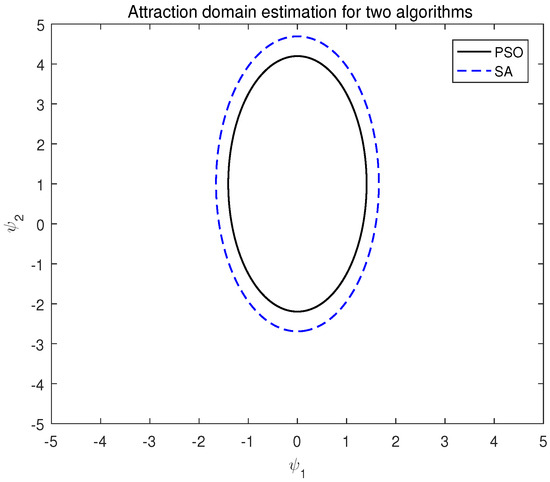
Figure 1.
Attraction domain estimation of two algorithms of system (13).
Remark 5.
Here is a concise introduction to the concepts of particle swarm optimization and simulated annealing algorithm. In the particle swarm algorithm, the transition probability from the system’s initial state to the desired target state is chosen as the fitness function. The individual optimal position, the global optimal position of the entire particle swarm, and each particle’s position and velocity are continuously updated until the optimal P is identified. The simulated annealing algorithm selects the transition probability from the system’s initial state to the desired target state as the objective function that needs to be optimized.
Example 2.
Consider the following 2D system with , , :
Taking the feedback control law for system (13), two different P-values are obtained by using the particle swarm optimization algorithm and the simulated annealing algorithm, respectively. Combined with the optimization problem, the attraction domain of the system under two different P-values is estimated. The optimization problem is the same as that of system (13). Here, we choose , .
P obtained by the particle swarm optimization is
Combined with the above, is obtained by Matlab.
P obtained by the simulated annealing algorithm is
Combined with the above, is obtained by Matlab. The attraction domain estimation of the two algorithms under system (13) is shown in Figure 2.
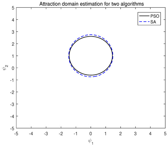
Figure 2.
Attraction domain estimation of two algorithms of system (14).
Example 3.
Consider the quantum system (15) with
Select the control law of system (13) and choose ,.
P obtained by the particle swarm optimization is
Combined with the above, is obtained by Matlab.
P obtained by the simulated annealing algorithm is
Combined with the above, is obtained by Matlab. The attraction domain estimation of the two algorithms under system (15) is shown in Figure 3.
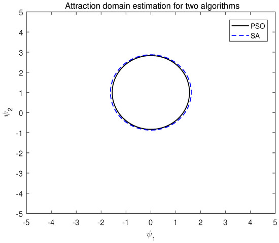
Figure 3.
Attraction domain estimation of two algorithms of system (15).
Example 4.
Consider the quantum system (16):
Select the control law of system (13) and choose , .
P obtained by the particle swarm optimization is
Combined with the above, is obtained by Matlab.
P obtained by the simulated annealing algorithm is
Combined with the above, is obtained by Matlab R2016a. The attraction domain estimation of the two algorithms under system (16) is shown in Figure 4.
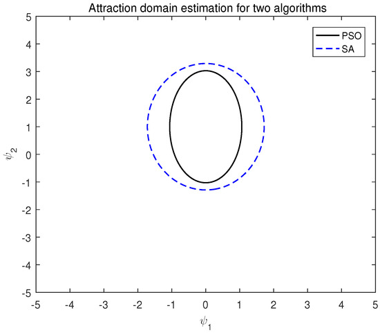
Figure 4.
Attraction domain estimation of two algorithms of system (16).
Example 5.
Consider the quantum system (17):
Select the control law of system (13) and choose , .
P obtained by the particle swarm optimization is
Combined with the above, is obtained by Matlab.
P obtained by the simulated annealing algorithm is
Combined with the above, is obtained by Matlab. The attraction domain estimation of the two algorithms under system (17) is shown in Figure 5.
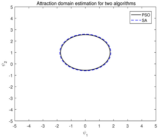
Figure 5.
Attraction domain estimation of two algorithms of system (17).
Example 6.
From all the above results, it can be seen that the size of the estimated attraction domain P-value obtained by the simulated annealing algorithm is larger than that of the domain estimated by the PSO algorithm. Example 6 is a spin particle system, where , , and are
Select the control law of system (13) and choose ,. P obtained by the particle swarm optimization is
Combined with the above, is obtained by Matlab.
P obtained by the simulated annealing algorithm is
Combined with the above, is obtained by Matlab. The attraction domain estimation of the two algorithms under system (18) is shown in Figure 6.
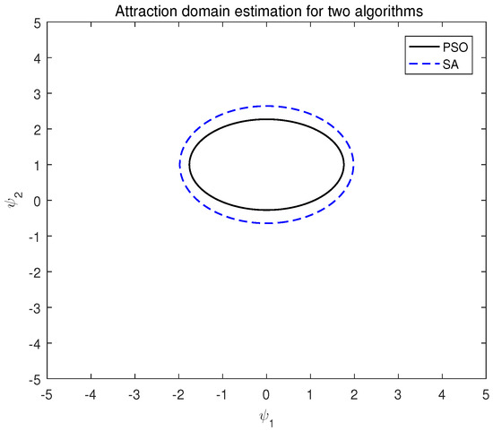
Figure 6.
Attraction domain estimation of two algorithms of system (18).
Based on the aforementioned results, it is evident that variations in the P-value significantly influence the system’s attraction domain. In these instances, the P-value derived from the simulated annealing algorithm yields a more expansive attraction domain for the system.
6. Conclusions
In this paper, we study the attraction domain estimation problem for a quantum system described by the Schrödinger equation. We provide stability conditions for nonlinear quantum systems and estimate the size of the attractor domain using the Lyapunov function method. Our approach transforms the attractor domain estimation into an optimization problem, specifically the minimization of the Lyapunov function on an ellipsoid. The quantum system in [8] employs a Lyapunov function based on the mean value of virtual mechanical quantities to construct the control law. We present two algorithms to solve for the mean value P of the virtual mechanical quantity: the PSO algorithm and the SAA. The primary focus of our research is to determine which of these two algorithms performs better. We estimate the attraction domain of quantum systems with P values obtained from different algorithms and conduct numerical simulations in various 2D test systems and spin 1/2 particle systems. The results indicate that the simulated annealing algorithm more effectively solves for the mean value P of the virtual mechanical quantity. Furthermore, the attracted region of the quantum system obtained through the SA algorithm is larger, signifying a greater locally asymptotically stable region.
Author Contributions
Methodology, I.G.I. and H.Y.; Formal analysis, I.G.I.; Investigation, H.Y. and G.Y.; Writing—original draft, H.Y.; Writing—review & editing, G.Y. All authors have read and agreed to the published version of the manuscript.
Funding
This research received no external funding.
Data Availability Statement
The original contributions presented in the study are included in the article, further inquiries can be directed to the corresponding authors.
Conflicts of Interest
The authors declare no conflicts of interest.
References
- He, W.K.; Li, S.Y. Enhancing topological information of the Lyapunov-based distributed model predictive control design for large-scale nonlinear systems. Asian J. Control 2022, 25, 1476–1487. [Google Scholar] [CrossRef]
- Liu, C.J.; Yang, J.; An, K.; Liu, M.; Chen, Q.J. Robust Control of Semi-passive Biped Dynamic Locomotion based on a Discrete Control Lyapunov Function. Robotica 2019, 38, 1345–1358. [Google Scholar] [CrossRef]
- Wang, J.; He, H.; Yu, J. Stabilization with guaranteed safety using Barrier Function and Control Lyapunov Function. J. Frankl. Inst. 2020, 357, 10472–10491. [Google Scholar] [CrossRef]
- Li, A.N.; Sun, J.T. Stability of nonlinear system under distributed Lyapunov-based economic model predictive control with time-delay. ISA Trans. 2020, 99, 148–153. [Google Scholar] [CrossRef] [PubMed]
- Rahmanei, H.; Aliabadi, A.; Ghaffari, A.; Azadi, S. Lyapunov-based control system design for trajectory tracking in electrical autonomous vehicles with in-wheel motors. J. Frankl. Inst. 2024, 361, 106736. [Google Scholar] [CrossRef]
- Ovchinnikov, M.; Mashtakov, Y.; Shestakov, S. Lyapunov-Based Control via Atmospheric Drag for Tetrahedral Satellite Formation. Mathematics 2024, 12, 189. [Google Scholar] [CrossRef]
- Liu, S.; Zhou, S.M.; Lu, X.J.; Gao, F.; Shuang, F.; Kuang, S. Lyapunov control of finite-dimensional quantum systems based on bi-objective quantum-behaved particle swarm optimization algorithm. J. Frankl. Inst. 2023, 360, 13951–13971. [Google Scholar] [CrossRef]
- Yu, G.H.; Yang, H.L. Quantum control based on three forms of Lyapunov functions. Chin. Phys. B 2024, 33, 1–7. [Google Scholar] [CrossRef]
- Zubov, V.I. Methods of A.M. Lyapunov and their application. Math. Comput. 1965, 19, 349. [Google Scholar]
- Davison, E.J.; Kurak, E.M. A computational method for determining quadratic lyapunov functions for non-linear systems. Automatica 1971, 7, 627–636. [Google Scholar] [CrossRef]
- Loparo, K.; Blankenship, G. Estimating the domain of attraction of nonlinear feedback systems. IEEE Trans. Autom. Control 1978, 23, 602–608. [Google Scholar] [CrossRef]
- Chiang, H.D.; Thorp, J.S. A constructive algorithm to estimate the stability regions of nonlinear dynamical systems. IEEE Int. Symp. Circuits Syst. 1988, 3, 2453–2456. [Google Scholar]
- Khalil, H.K. Nonlinear Systems, 3rd ed.; Prentice Hall Inc.: Upper Saddle River, NJ, USA, 2002. [Google Scholar]
- Chang, F.Y.; Cui, X.F.; Wang, M.Q.; Su, W.C. Region of Attraction Estimation for DC Microgrids With Constant Power Loads Using Potential Theory. IEEE Trans. Smart Grid 2021, 12, 3793–3808. [Google Scholar] [CrossRef]
- Nishino, T.; Ishizaki, T. Estimation of Domain of Attraction Based on Equilibrium-Independent Passivity of Power Systems. IFAC PapersOnLine 2023, 56, 2299–2304. [Google Scholar] [CrossRef]
- Valmorbida, G.; Anderson, J. Region of attraction estimation using invariant sets and rational Lyapunov functions. Automatica 2017, 75, 37–45. [Google Scholar] [CrossRef]
- Vannelli, A.; Vidyasagar, M. Maximal Lyapunov Functions and Domains of Attraction for Autonomous Nonlinear Systems. IFAC Proc. Vol. 1981, 14, 117–122. [Google Scholar] [CrossRef]
- Pesterev, A.V. Estimation of the Attraction Domain for an Affine System with Constrained Vector Control Closed by the Linearizing Feedback. Autom. Remote Control 2019, 80, 840–855. [Google Scholar] [CrossRef]
- Kaouther, M.; Mirko, F.; Mazen, A. Probabilistically certified region of attraction of a tumor growth model with combined chemo- and immunotherapy. Int. J. Robust Nonlinear Control 2022, 32, 6539–6555. [Google Scholar]
- Liu, Y.; Zhang, J.; Chen, S.; Yu, X.D. Stability analysis and estimation of domain of attraction for hydropower station with surge tank. Chaos Solitons Fractals Interdiscip. J. Nonlinear Sci. Nonequilibrium Complex Phenom. 2023, 170, 113–413. [Google Scholar] [CrossRef]
- Zhou, Y.; Li, J.D.; Sun, M.W.; Zhang, J.H.; Chen, Z.Q. Cascade control design for supercavitating vehicles with actuator saturation and the estimation of the domain of attraction. Ocean Eng. 2023, 282, 114996. [Google Scholar] [CrossRef]
- Platonov, A.V. Stability conditions and estimation of the region of attraction for a class of nonlinear switched systems. Int. J. Dyn. Control 2022, 10, 1442–1450. [Google Scholar] [CrossRef]
- Wu, H.J.; Li, C.D.; He, Z.L.; Wang, Y.N. Estimation of attraction domain of nonlinear systems with saturated impulses and input disturbances. Int. J. Robust Nonlinear Control 2021, 31, 9466–9482. [Google Scholar] [CrossRef]
- Jin, D.Q.; Yu, L. An Improved Approach for Estimating Attraction Domain. Sci. Technol. Vis. 2018, 6, 187–188. [Google Scholar]
- Hahn, W. Stability of Motion; Springer: Berlin/Heidelberg, Germany, 1967. [Google Scholar]
- LaSalle, J.; Lefschetz, S. Stability by Liapunov’s Direct Method with Applications; Academic Press: New York, NY, USA; London, UK, 1961. [Google Scholar]
- Hong, Y.G.; Cheng, D.Z. Analysis and Control of Nonlinear Systems; Science Press: Beijing, China, 2005. [Google Scholar]
- Ichikawa, K.; Ortega, R. On stabilization of nonlinear systems with enlarged domain of attraction. Automatica 1992, 28, 623–626. [Google Scholar] [CrossRef]
- Coron, J.M.; Grigoriu, A.; Lefter, C.; Turinici, G. Quantum control design by Lyapunov trajectory tracking for dipole and polarizability coupling. New J. Phys. 2009, 11, 105034. [Google Scholar] [CrossRef]
- Kuang, S.; Cong, S. Lyapunov control methods of closed quantum systems. Automatica 2008, 44, 98–108. [Google Scholar] [CrossRef]
Disclaimer/Publisher’s Note: The statements, opinions and data contained in all publications are solely those of the individual author(s) and contributor(s) and not of MDPI and/or the editor(s). MDPI and/or the editor(s) disclaim responsibility for any injury to people or property resulting from any ideas, methods, instructions or products referred to in the content. |
© 2024 by the authors. Licensee MDPI, Basel, Switzerland. This article is an open access article distributed under the terms and conditions of the Creative Commons Attribution (CC BY) license (https://creativecommons.org/licenses/by/4.0/).