Optimal Investment Strategy for DC Pension Plan with Stochastic Salary and Value at Risk Constraint in Stochastic Volatility Model

Abstract

This paper studies the optimal asset allocation problem of a defined contribution (DC) pension plan with a stochastic salary and value under a constraint within a stochastic volatility model. It is assumed that the financial market contains a risk-free asset and a risky asset whose price process satisfies the Stein–Stein stochastic volatility model. To comply with regulatory standards and offer a risk management tool, we integrate the dynamic versions of Value-at-Risk (VaR), Conditional Value-at-Risk (CVaR), and worst-case CVaR (wcCVaR) constraints into the DC pension fund management model. The salary is assumed to be stochastic and characterized by geometric Brownian motion. In the dynamic setting, a CVaR/wcCVaR constraint is equivalent to a VaR constraint under a higher confidence level. By using the Lagrange multiplier method and the dynamic programming method to maximize the constant absolute risk aversion (CARA) utility of terminal wealth, we obtain closed-form expressions of optimal investment strategies with and without a VaR constraint. Several numerical examples are provided to illustrate the impact of a dynamic VaR/CVaR/wcCVaR constraint and other parameters on the optimal strategy.

1. Introduction

With the growth in both the size and proportion of older persons in the population, managing pension funds becomes increasingly crucial in the social security system. The primary features of a pension fund are the contributions from the active workers and the benefits provided to the retirees. There are generally two types of pension plan worldwide. One is the defined benefit (DB) pension plan, in which the benefits are determined in advance by the sponsor. The contributions are initially set and adjusted as needed to maintain fund balance. The other is the defined contribution (DC) pension plan, where the contributions are fixed and the retirement benefits depend on the accumulated fund wealth at the time of retirement. However, DC pension plans offer the benefit of alleviating pressure on the social security system while shifting investment and longevity risks from plan sponsors to the members. Therefore, solving the problem of the optimal investment strategy for a DC pension plan is of great theoretical and practical value. Many works of literature studied the optimal management of DC pension funds. See [1,2,3,4,5,6,7,8,9,10] for details.

It is well-known that the salaries of DC pension plan participants are periodically adjusted based on economic conditions. Contributions typically depend on the participant’s salary, which is stochastic. This salary volatility risk can be influenced by factors such as economic cycles, industry shifts, and labor market conditions, leading to discrepancies between participants’ actual and expected salaries. Some scholars have investigated the optimal investment problem for DC pension plans considering stochastic salaries. For example, Guan and Liang [11] modeled salary using a stochastic process and studied the optimal asset allocation problem for DC pension funds under S-shaped utility. Sun et al. [6] sought the robust optimal investment strategy for DC pension funds with ambiguity aversion and stochastic salaries. Yan et al. [12] examined a robust optimal investment problem for a DC pension plan with a return of premiums clause, accounting for both inflation and salary risks. Chang et al. [13] investigated robust equilibrium investment strategies for DC pension funds, taking into account both the stochastic volatility and stochastic income under the mean-variance criteria.

However, in most of the aforementioned papers, the price process of the risky asset is modeled using geometric Brownian motion (GBM), which assumes that the volatility of the asset’s price remains constant and deterministic. This assumption contradicts empirical evidence, which shows that historical volatility tends to fluctuate over time. Consequently, an increasing number of scholars are turning their attention from the GBM to the stochastic volatility (SV) model, with the SV model acknowledged as a significant aspect of the pricing process for risky assets. For instance, Gao [14] and Wang et al. [15] derived the optimal investment strategy for DC pension funds, as the price process of the risky asset follows the constant elasticity of variance (CEV) model. Similarly, Zhao and Rong [16], Guan and Liang [17], and Ma et al. [18] investigated the optimal portfolios for DC pension funds under the Heston stochastic volatility model (where volatility follows the Cox–Ingersoll–Ross process). He and Zhu [19] and Lin et al. [20] studied the option pricing problem under the Stein–Stein model (where volatility follows the Ornstein–Uhlenbeck process). Consequently, it is essential to incorporate stochastic volatility into the investment management of DC pension funds.

With the rapid development of the financial market, pension funds face significant exposure to risk. Value-at-Risk (VaR) has emerged as a standard tool for measuring and controlling risks. VaR estimates the maximum expected loss over a specified period at a predetermined confidence level. However, VaR has some undesirable theoretical properties. For instance, Artzner et al. [21] demonstrated that VaR is not a coherent risk measure because it does not fulfill the subadditivity property. Basak and Shapiro [22] found that tail expectation-based measures are preferable to quantile-based measures (such as VaR) in terms of controlling risks. As a result, Conditional Value-at-Risk (CVaR), also known as conditional tail expectation (CTE) and average Value-at-Risk (AVaR), is a convex and coherent risk measure frequently recommended as an alternative to Value-at-Risk (VaR). CVaR, which incorporates elements of VaR while providing additional insight into the tail distribution of returns, represents the expected loss in the worst-case scenarios of a specified percentile. To address the issue of incomplete information on loss distribution, recent research has focused on worst-case scenario risk measures, particularly worst-case Value-at-Risk (wcVaR) and worst-case Conditional Value-at-Risk (wcCVaR). Čerbáková [23] highlighted that wcVaR and wcCVaR are identical when the distribution is identified by its first two moments. Additionally, Natarajan et al. [24] affirmed that wcCVaR is a coherent risk measure.

In recent years, some scholars have used risk measurement technology to measure and control the risk of trading portfolios. For example, Yiu [25] applied a dynamic programming method to solve the optimal investment and consumption problem under the dynamic VaR constraint. Cuoco et al. [26] formulated a dynamically consistent model of optimal portfolio choice subject to a VaR constraint. They found that the risk exposure of a trader under the VaR constraint is consistently lower than that of an unconstrained trader, leading to a reduced probability of extreme losses. Zhang et al. [27] examined the optimal reinsurance strategy within proportional and excess-of-loss frameworks, considering dynamic VaR, CVaR, and wcCVaR constraints. Zhang and Gao [28] studied the problem of dynamic portfolio selection based on a benchmark process and dynamic Value-at-Risk constraint. Dong et al. [29] investigated an optimal investment problem for a DC pension plan, incorporating both a VaR constraint and an expected shortfall constraint. In this paper, we adopt three dynamic risk metrics, dynamic VaR, CVaR, and wcCVaR, to establish constraints on the wealth of DC pension funds.

This paper investigates optimal investment strategies for DC pension funds with stochastic salary and VaR constraint under a stochastic volatility model. The fund managers allocate accumulated pension funds in the financial market comprising a risk-free asset and a risky asset, characterized by the Stein–Stein stochastic volatility model. The salary of DC pension plan participants is assumed to follow geometric Brownian motion. The objective of the fund managers is to maximize the expected utility of the terminal wealth. Within a dynamic setting, it is always feasible to transform a CVaR/wcCVaR constraint into an equivalent VaR limit. Consequently, the optimization problem governed by a dynamic CVaR/wcCVaR constraint can be restructured to fit a dynamic VaR constraint with a higher confidence level. By applying the dynamic programming principle and the Lagrange multiplier method, optimal investment strategies are derived both with and without the dynamic VaR constraint. Numerical examples illustrate how dynamic VaR/CVaR/wcCVaR constraints and various parameters impact optimal investment strategies.

The contributions of this paper are as follows. Firstly, we introduce the dynamic version of the Value-at-Risk (VaR), Conditional Value-at-Risk (CVaR) and worst-case CVaR (wcCVaR) constraints in a DC pension fund management model. Secondly, we investigate the optimal investment strategies for DC pension funds with stochastic salary and a stochastic volatility model under dynamic VaR, CVaR and wcCVaR constraints. Finally, numerical analyses show that considering a dynamic VaR constraint can effectively improve the risk management level of pension funds, ensuring that fund assets are better equipped to handle market fluctuations.

The rest of this paper is organized as follows. In Section 2, we present the model and assumptions about the financial market. In Section 3, we solve the optimization problem without a VaR constraint. By constructing and solving the HJB equation, we obtain the explicit solution of the optimal investment strategy. In Section 4, we introduce dynamic VaR, CVaR and wcCVaR constraints and solve the optimization problem with a dynamic VaR constraint. Numerical illustrations are provided in Section 5. Section 6 concludes the paper. Some proofs are given in Appendix A, Appendix B and Appendix C.

2. Model and Assumptions

Fund managers can trade continuously in the financial market without extra costs or taxes. Let $(\mathsf{\Omega },\mathcal{F},\mathrm{P})$ be a complete probability space with filtration ${\left\{{\mathcal{F}}_t\right\}}_{t\in [0,T]}$, where ${\mathcal{F}}_t$ is the information of the market available up to time t. $T>0$ represents the time horizon. All stochastic processes and random variables are well-defined on the probability space, and any decision made at time t is based on ${\mathcal{F}}_t$.

2.1. Financial Market

We assume that the financial market consists of a risk-free asset and a risky asset (stock). The price process of the risk-free asset $S_0\left(t\right)$ is given by the following equation:

$$\mathrm{d}{S}_0\left(t\right)=r_0{S}_0\left(t\right)\mathrm{dt},{\mathrm{S}}_0\left(0\right)={\mathrm{s}}_0,$$

(1)

where $r_0$ represents a risk-free interest rate.

The price of the risky asset $S_1\left(t\right)$ is described by the Stein–Stein stochastic volatility model:

$$\begin{array}{c}{\displaystyle \frac{\mathrm{d}{S}_1\left(t\right)}{S_1\left(t\right)}}=r_0\mathrm{d}t+\left|V\left(t\right)\right|(\xi \mathrm{d}t+\mathrm{d}W\left(t\right)),S_1\left(0\right)=s_1,\hfill \end{array}$$

(2)

$$\begin{array}{c}\mathrm{d}V\left(t\right)=k(\theta -V\left(t\right))\mathrm{d}t+\sigma \mathrm{d}{W}_v\left(t\right),V\left(0\right)=v_0.\hfill \end{array}$$

(3)

Equation (3) is the Ornstein–Uhlenbeck (O-U) process, which exhibits mean-reverting properties. $\xi >0$ is a constant, and $\xi V\left(t\right)$ represents the risk compensation for the Brownian motion $W\left(t\right)$. $\theta >0$ indicates the long-term mean of $V\left(t\right)$. $k>0$ is the rate of mean reversion. $\sigma$ is the volatility of $V\left(t\right)$. $W\left(t\right)$ and $W_v\left(t\right)$ are correlated standard Brownian motions, and it is assumed that $\mathrm{E}\left[\mathrm{d}W\left(t\right)\mathrm{d}{W}_v\left(t\right)\right]=\rho \mathrm{d}t$, where $\rho \in [-1,1]$ is the correlation coefficient.

2.2. Wealth Process

The participants in the DC pension plan consistently contribute a set percentage of their salaries to the pension fund and receive benefits upon retirement. Since salaries are often subject to uncertainties due to macroeconomic influences, it is more realistic to consider the salary described through a stochastic process. We represent the salary at time t as $Y\left(t\right)$, which satisfies the following stochastic differential equation:

$$\begin{array}{c}\hfill {\displaystyle \frac{\mathrm{d}Y\left(t\right)}{Y\left(t\right)}}=(r_0+\mu )\mathrm{d}t+{\sigma }_y\mathrm{d}W\left(t\right),Y\left(0\right)=y_0,\end{array}$$

(4)

where $r_0+\mu$ represents the expected instantaneous growth rate of the salary, which consists of two components: $r_0$ and $\mu$. The term $r_0$ reflects the influence of the macroeconomic environment and suggests that the salary growth of plan participants is dependent on the interest rate in the financial market. Meanwhile, the constant $\mu$ represents the salary growth of plan participants that can be attributed to inflation or increases in benefits. Additionally, ${\sigma }_y>0$ represents the volatility.

Remark 1. 

In Equation (4), notice that salary is influenced by the financial market (i.e., stocks). This implies that ${\sigma }_y$ is a hedgeable volatility, with its risk source belonging to the financial market. This assumption is consistent with the findings of [30,31,32,33,34].

Remark 2. 

Given the typically long investment horizon of a DC pension fund, a stochastic salary model more accurately reflects the real-world operations of pension plans. The variability in salary, driven by its stochastic nature, is what causes fluctuations in the contribution rate.

We assume that participants in the DC pension plan consistently contribute a fixed proportion, denoted as p, of their salaries to the pension fund until retirement. Define $\pi \left(t\right)$ as the amount invested in the risky asset at time t, while the remainder is allocated to the risk-free asset. Let $F\left(t\right)$ represent the total wealth in the pension fund account at time t under the strategy $\pi \left(t\right)$, then $F\left(t\right)$ satisfies the following stochastic differential equation:

$$\begin{array}{c}\hfill \left\{\begin{array}{cc}\mathrm{d}F\left(t\right)\hfill & =(F\left(t\right)-\pi \left(t\right)){\displaystyle \frac{\mathrm{d}{S}_0\left(t\right)}{S_0\left(t\right)}}+\pi \left(t\right){\displaystyle \frac{\mathrm{d}S\left(t\right)}{S\left(t\right)}}+pY\left(t\right)\mathrm{d}t\hfill \\ & =[r_{0}F\left(t\right)+\xi |V\left(t\right)|\pi \left(t\right)+pY\left(t\right)]\mathrm{d}t+\pi \left(t\right)\left|V\left(t\right)\right|\mathrm{d}W\left(t\right),\hfill \\ F\left(0\right)\hfill & =f_0.\hfill \end{array}\right.\end{array}$$

(5)

Definition 1. 

We refer to the strategy ${\pi \left(t\right)}_{t\in [0,T]}$ as an admissible strategy if $\mathrm{E}\left({\int }_0^T{\pi }^2\left(t\right)\mathrm{d}t\right)<\infty$ and the Equation (5) has a pathwise unique solution ${\left\{F\left(t\right)\right\}}_{t\in [0,T]}$.

Let $\Pi$ denote the set of all admissible strategies.

3. Optimal Strategy without Dynamic VaR Constraint

We suppose that the pension fund managers are concerned about the total wealth in the pension fund account. The more pension fund wealth accumulated in the account, the higher the pension plan participants will receive at the retirement. Therefore, we assume the goal of the fund managers to be maximizing the expected utility of their terminal wealth. The optimization problem can be formulated as follows:

$$\left\{\begin{array}{c}\underset{\pi \in \Pi }{max}E\left[U\right(F\left(T\right)\left)\right]\hfill \\ \mathrm{s}.\mathrm{t}.F\left(t\right)satisfies\left(5\right).\hfill \end{array}\right.$$

(6)

The value function is defined as

$$H(t,f,v,y)=\underset{\pi \in \Pi }{sup}{\mathrm{E}}_{t,f,v,y}\left[U\left(F\left(T\right)\right)\right].$$

(7)

Here, ${\mathrm{E}}_{t,f,v,y}[·]=\mathrm{E}[·\mid F\left(t\right)=f,V\left(t\right)=v,Y\left(t\right)=y]$ represents the conditional expectation given the total wealth $F\left(T\right)$ at terminal time T under strategy $\pi$, the value $V\left(t\right)$, and the value $Y\left(t\right)$. $U(·)$ denotes the utility function.

The Hamilton–Jacobi–Bellman (HJB) equation associated with the optimization problem is

$$\begin{array}{c}{H}_t+\underset{\pi \in \Pi }{sup}\{\left[f{r}_0+\xi \left|v\right|\pi \left(t\right)+py\right]H_f+{\displaystyle \frac{1}{2}}{v}^2{\pi }^2\left(t\right)H_{ff}+\sigma \rho \left|v\right|\pi \left(t\right)H_{fv}+k(\theta -v)H_v\hfill \\ +{\displaystyle \frac{1}{2}}{\sigma }^2{H}_{vv}+y(r_0+\mu )H_y+{\displaystyle \frac{1}{2}}{\sigma }_y^2{y}^2{H}_{yy}+\left|v\right|\pi \left(t\right){\sigma }_{y}y{H}_{fy}+\rho \sigma {\sigma }_{y}y{H}_{vy}\}=0.\hfill \end{array}$$

(8)

Here, $H_t,H_f,H_v,H_y,H_{ff},H_{vv},H_{fv},H_{fy},H_{vy},H_{yy}$ are partial derivatives of first and second orders of the value function H with respect to the corresponding variables.

The first-order condition for the optimal investment strategy ${\pi }^{*}\left(t\right)$ satisfies:

$${\pi }^{*}\left(t\right)={\displaystyle \frac{-\xi H_f-\sigma \rho H_{fv}-{\sigma }_{y}y{H}_{fy}}{\left|v\right|H_{ff}}}.$$

(9)

Suppose that the fund managers adopt the exponential utility function $U\left(x\right)=-{\displaystyle \frac{1}{m}}{\mathrm{e}}^{-mx}$, where $m>0$ represents the risk aversion coefficient of the fund managers. Therefore, we conjecture a solution to the Equation (8) as follows:

$$H(t,f,v,y)=-{\displaystyle \frac{1}{m}}{\mathrm{e}}^{-m\left[A\right(t)+B(t)f+C(t)v+D(t\left)y\right]},$$

with the boundary conditions given by $A\left(T\right)=0,B\left(T\right)=1,C\left(T\right)=0,D\left(T\right)=0$. Hence, we have

$$\begin{array}{c}{H}_t=-m\left(A_t+B_{t}f+C_{t}v+D_{t}y\right)H,H_f=-mB\left(t\right)H,H_v=-mC\left(t\right)H,\\ H_y=-mD\left(t\right)H,H_{ff}=m^2{B}^2\left(t\right)H,H_{yy}=m^{2}D{\left(t\right)}^{2}H,H_{vv}=m^2{C}^2\left(t\right)H,\\ H_{fv}=m^{2}B\left(t\right)C\left(t\right)H,H_{fy}=m^{2}B\left(t\right)D\left(t\right)H,H_{vy}=m^{2}C\left(t\right)D\left(t\right)H.\end{array}$$

(10)

Next, we put (10) into (9) to obtain

$${\pi }^{*}\left(t\right)={\displaystyle \frac{\xi -\sigma \rho mC\left(t\right)-{\sigma }_{y}ymD\left(t\right)}{mB\left(t\right)\left|v\right|}}.$$

(11)

By substituting (10) and (11) into (8), we obtain

$$\begin{array}{c}-m(A_t+B_{t}f+C_{t}v+D_{t}y)H-[f{r}_0+\xi {\displaystyle \frac{\xi -\sigma \rho mC\left(t\right)-{\sigma }_{y}ymD\left(t\right)}{mB\left(t\right)}}+py]mB\left(t\right)H\hfill \\ -k(\theta -v)mC\left(t\right)H+{\displaystyle \frac{1}{2}}{[\xi -\sigma \rho mC\left(t\right)-{\sigma }_{y}ymD\left(t\right)]}^{2}H+{\displaystyle \frac{1}{2}}{\sigma }^2{m}^2{C}^2\left(t\right)H\hfill \\ +\sigma \rho mC\left(t\right)H[\xi -\rho \sigma mC\left(t\right)-{\sigma }_{y}ymD\left(t\right)]-y(r_0+\mu )mD\left(t\right)H+{\displaystyle \frac{1}{2}}{\sigma }_y^2{m}^2{D}^2\left(t\right)y^{2}H\hfill \\ +(\xi -\sigma \rho mC\left(t\right)-{\sigma }_{y}ymD\left(t\right)){\sigma }_{y}ymD\left(t\right)H+\sigma \rho mC\left(t\right){\sigma }_{y}ymD\left(t\right)H=0.\hfill \end{array}$$

(12)

By separating variables in the above equation with respect to $f,v,y$, and other terms, we obtain the following equations.

$$\begin{array}{c}-m{B}_t-m{r}_{0}B\left(t\right)=0,\hfill \end{array}$$

(13)

$$\begin{array}{c}-m{C}_t+kmC\left(t\right)=0,\hfill \end{array}$$

(14)

$$\begin{array}{c}-m{D}_t+\xi {\sigma }_{y}mD\left(t\right)-pmB\left(t\right)-(r_0+\mu )mD\left(t\right)=0,\hfill \end{array}$$

(15)

$$\begin{array}{c}-m{A}_t-\xi (\xi -\sigma \rho mC\left(t\right))-k\theta mC\left(t\right)+{\displaystyle \frac{1}{2}}{[\xi -\sigma \rho mC\left(t\right)]}^2+{\displaystyle \frac{1}{2}}{\sigma }^2{m}^2{C}^2\left(t\right)+\sigma \rho mC\left(t\right)[\xi -\rho \sigma mC\left(t\right)]=0.\hfill \end{array}$$

(16)

Taking the boundary conditions $A\left(T\right)=0,B\left(T\right)=1,C\left(T\right)=0$ and $D\left(T\right)=0$ into account, the solutions of the above equations are as follows:

$$\begin{array}{c}A\left(t\right)={\displaystyle \frac{{\xi }^2}{2m}}(T-t),B\left(t\right)={\mathrm{e}}^{r_0(T-t)},\\ C\left(t\right)=0,D\left(t\right)={\displaystyle \frac{p}{\mu -{\sigma }_y\xi }}\left({\mathrm{e}}^{\left(r_0+\mu -\xi {\sigma }_y\right)(T-t)}-{\mathrm{e}}^{r_0(T-t)}\right).\end{array}$$

(17)

Therefore, the optimal investment strategy and the corresponding optimal value function are respectively

$${\pi }^{*}\left(t\right)={\displaystyle \frac{\xi -{\sigma }_{y}mD\left(t\right)y}{mB\left(t\right)\left|v\right|}},H(t,f,v,y)=-{\displaystyle \frac{1}{m}}{\mathrm{e}}^{-m\left[A\right(t)+B(t)f+D(t\left)y\right]}.$$

(18)

Remark 3. 

When we substitute the optimal investment strategy ${\pi }^{*}\left(t\right)$ into the wealth process Equation (5), we observe that the volatility term $\left|V\right(t\left)\right|$ is cancelled out. This suggests that, according to this criterion, the value function’s specific value does not depend on the volatility $\left|V\right(t\left)\right|$. Furthermore, it implies that under the assumed market conditions, the optimal investment strategy can completely hedge against the stochastic volatility risk of the risky asset.

4. Optimal Strategy with Dynamic VaR Constraint

In this section, we study the optimal investment strategy of the optimization problem under dynamic VaR constraint.

4.1. Dynamic VaR, CVaR and wcCVaR

The investment of DC pension fund focuses on achieving long-term, steady growth. The fund managers utilize the VaR risk measure to manage wealth and prevent significant losses. Motivated by [25,26,35], we formulate the dynamic VaR and CVaR constraint of the fund wealth. We suppose that within a minuscule time span $\tau$, the fund manager ignores the changes in portfolio, stock price volatility, and salaries, i.e., $\pi \left(l\right)=\pi \left(t\right),V\left(l\right)=V\left(t\right),Y\left(l\right)=Y\left(t\right),l\in [t,t+\tau ]$. This implies that in computing the VaR, the amount invested in the risky asset is always maintained at $\pi \left(t\right)$ within the interval $[t,t+\tau ]$, the volatility of the stock remains constant at $\left|V\right(t\left)\right|$, and the salary is held steady at $Y\left(t\right)$. This assumption is reasonable because in practice the fund managers usually adjust its investment strategy on a monthly (quarterly or yearly) basis and salaries are adjusted on a monthly (quarterly or yearly) basis.

Although the adjustment of investment decision and salary process may not be synchronous, as long as $\tau$ is small enough, the investment strategy and salary process can always be adjusted synchronously. Thus, the loss of the fund managers in time interval $[t,t+\tau ]$ can be expressed as $\Delta F\left(t\right)=F\left(t\right){\mathrm{e}}^{r_0\tau }-F(t+\tau ).$ According to the Itô’s formula, the SDE (5) can be rewritten as

$$F\left(t\right)=F\left(0\right){\mathrm{e}}^{r_{0}t}+{\int }_0^t{\mathrm{e}}^{r_0(t-u)}\left[\xi \left|V\right(u\left)\right|\pi \left(u\right)+pY\left(u\right)\right]\mathrm{d}u+{\int }_0^t{\mathrm{e}}^{r_0(t-u)}\pi \left(u\right)\left|V\left(u\right)\right|\mathrm{d}W\left(u\right).$$

(19)

When $s>t$, the above equation can be expressed as follows,

$$\begin{array}{c}\hfill F\left(s\right)=F\left(t\right){\mathrm{e}}^{r_0(s-t)}+{\int }_t^s{\mathrm{e}}^{r_0(s-u)}\left[\xi \left|V\right(u\left)\right|\pi \left(u\right)+pY\left(u\right)\right]\mathrm{d}u+{\int }_t^s{\mathrm{e}}^{r_0(s-u)}\pi \left(u\right)\left|V\left(u\right)\right|\mathrm{d}W\left(u\right).\end{array}$$

(20)

Thus,

$$\begin{array}{cc}\hfill \Delta F\left(t\right)=& -\xi \left|V\left(t\right)\right|\pi \left(t\right){\int }_t^{t+\tau }{\mathrm{e}}^{r_0(t+\tau -u)}\mathrm{d}u-{\int }_t^{t+\tau }{\mathrm{e}}^{r_0(t+\tau -u)}pY\left(u\right)\mathrm{d}u\hfill \\ & -\pi \left(t\right)\left|V\left(t\right)\right|{\int }_t^{t+\tau }{\mathrm{e}}^{r_0(t+\tau -u)}\mathrm{d}W\left(u\right)\hfill \\ \hfill =& \xi \left|V\left(t\right)\right|\pi \left(t\right){\displaystyle \frac{1-{\mathrm{e}}^{r_0\tau }}{r_0}}+pY\left(t\right){\displaystyle \frac{1-{\mathrm{e}}^{r_0\tau }}{r_0}}-\pi \left(t\right)\left|V\left(t\right)\right|{\int }_t^{t+\tau }{\mathrm{e}}^{r_0(t+\tau -u)}\mathrm{d}W\left(u\right).\hfill \end{array}$$

(21)

One feasible way to control its wealth risk for the fund manager is to control the VaR of $\Delta F\left(t\right)$ for any $t\in [0,T]$ with a small time step $\tau$, such as $\tau =1/365$ (any day), $\tau =1/250$ (any trading day), $\tau =1/52$ (any week), $\tau =1/12$ (any month), $\tau =1/4$ (any quarter), and $\tau =1$ (any year).

For a given confidence level $1-\beta$, where $\beta \in [0,1]$, and a given horizon $\tau >0$, we define the VaR at time t of the fund wealth, denoted by ${\mathrm{VaR}}_t^{\beta ,\tau }$, as follows:

$${\mathrm{VaR}}_t^{\beta ,\tau }=inf\left\{M⩾0:P\left(\Delta F\left(t\right)\ge M|{\mathcal{F}}_t\right)⩽\beta \right\}.$$

(22)

In other words, ${\mathrm{VaR}}_t^{\beta ,\tau }$ represents the maximum possible loss over the forthcoming time period of length $\tau$ at the confidence level $1-\beta$. It is adopted by regulators to set capital requirements for an institution. Thus, many studies use VaR as a constraint in their optimization problems.

CVaR, which incorporates elements of VaR while providing additional insight into the tail distribution of returns, represents the expected loss in the worst-case scenarios of a specified percentile. The dynamic Conditional Value-at-Risk ${\mathrm{CVaR}}_t^{\beta ,\tau }$ is then given by

$${\mathrm{CVaR}}_t^{\beta ,\tau }=\mathbb{E}[\Delta F\left(t\right)\mid \Delta F\left(t\right)\ge {\mathrm{VaR}}_t^{\beta ,\tau }].$$

(23)

When distribution information is incomplete, worst-case strategies like wcVaR and wcCVaR are employed. The definition and properties of worst-case CVaR have been studied by [24,36]. Below, we introduce a dynamic version of wcCVaR. The set ${\mathcal{P}}_1$ of feasible probability distributions is defined as follows:

$$\begin{array}{c}{\mathcal{P}}_1= \{p(·):{\mathbb{E}}_p[\Delta F\left(t\right)]=\xi \left|V\left(t\right)\right|\pi \left(t\right){\displaystyle \frac{1-{\mathrm{e}}^{r_0\tau }}{r_0}}+pY\left(t\right){\displaystyle \frac{1-{\mathrm{e}}^{r_0\tau }}{r_0}},\hfill \\ {\mathbb{E}}_p\left[{(\Delta F\left(t\right))}^2\right]={\displaystyle \frac{{\mathrm{e}}^{2r_0\tau }-1}{2r_0}}{\pi }^2\left(t\right)V^2\left(t\right)+\left(\xi \right|V\left(t\right)|\pi \left(t\right){\displaystyle \frac{1-{\mathrm{e}}^{r_0\tau }}{r_0}}+pY\left(t\right){\displaystyle \frac{1-{\mathrm{e}}^{r_0\tau }}{r_0}}{)}^2\},\hfill \end{array}$$

(24)

and the dynamic worst-case Conditional Value-at-Risk, denoted by ${\mathrm{wcCVaR}}_t^{\beta ,\tau }$ is defined as

$$\begin{array}{c}\hfill {\mathrm{wcCVaR}}_t^{\beta ,\tau }=\underset{p(·)\in {\mathcal{P}}_1}{sup}\underset{a\in \mathbb{R}}{inf}\left\{a+{\displaystyle \frac{1}{\beta }}{\mathbb{E}}_p\left[{(\Delta F\left(t\right)-a)}^{+}\right]\right\},\end{array}$$

(25)

where ${\left(x\right)}^{+}=max\{0,x\}$ and the subscript p indicates that expectation is calculated under distribution $p(·)$.

Using the above definitions, we offer the following lemma.

Lemma 1. 

For the wealth process described by Equation (5), given a time horizon τ and a confidence level $1-\beta$, the VaR at time t can be expressed as:

$${\mathrm{VaR}}_t^{\beta ,\tau }={\left\{\xi \left|V\left(t\right)\right|\pi \left(t\right){\displaystyle \frac{1-{\mathrm{e}}^{r_0\tau }}{r_0}}+pY\left(t\right){\displaystyle \frac{1-{\mathrm{e}}^{r_0\tau }}{r_0}}-{\mathsf{\Phi }}^{-1}\left(\beta \right)\sqrt{{\displaystyle \frac{{\mathrm{e}}^{2r_0\tau }-1}{2r_0}}}\left|\pi \left(t\right)\right|\left|V\left(t\right)\right|\right\}}^{+},$$

(26)

and the CVaR at time t can be expressed as:

$${\mathrm{CVaR}}_t^{\beta ,\tau }={\left\{\xi \left|V\left(t\right)\right|\pi \left(t\right){\displaystyle \frac{1-{\mathrm{e}}^{r_0\tau }}{r_0}}+pY\left(t\right){\displaystyle \frac{1-{\mathrm{e}}^{r_0\tau }}{r_0}}+{\displaystyle \frac{\varphi \left({\mathsf{\Phi }}^{-1}\left(\beta \right)\right)}{\beta }}\sqrt{{\displaystyle \frac{{\mathrm{e}}^{2r_0\tau }-1}{2r_0}}}\left|\pi \left(t\right)\right|\left|V\left(t\right)\right|\right\}}^{+},$$

(27)

where $\varphi \left(x\right)$ and $\mathsf{\Phi }\left(x\right)$ represent the probability density function and the cumulative distribution function of a standard normal random variable, respectively. The inverse function of $\mathsf{\Phi }\left(x\right)$ is denoted by ${\mathsf{\Phi }}^{-1}\left(x\right)$. The dynamic wcCVaR can be expressed as:

$${\mathrm{wcCVaR}}_t^{\beta ,\tau }={\left\{\xi \left|V\left(t\right)\right|\pi \left(t\right){\displaystyle \frac{1-{\mathrm{e}}^{r_0\tau }}{r_0}}+pY\left(t\right){\displaystyle \frac{1-{\mathrm{e}}^{r_0\tau }}{r_0}}+\sqrt{{\displaystyle \frac{1-\beta }{\beta }}}\sqrt{{\displaystyle \frac{{\mathrm{e}}^{2r_0\tau }-1}{2r_0}}}\left|\pi \left(t\right)\right|\left|V\left(t\right)\right|\right\}}^{+}.$$

(28)

In particular,

$$0\le {\mathrm{VaR}}_t^{\beta ,\tau }\le {\mathrm{CVaR}}_t^{\beta ,\tau }\le {\mathrm{wcCVaR}}_t^{\beta ,\tau }<F\left(t\right).$$

(29)

Proof. 

The proof is provided in Appendix A. □

Remark 4. 

We have ${\mathrm{CVaR}}_t^{\beta ,\tau }={\mathrm{VaR}}_t^{\tilde{\beta },\tau }$ and ${\mathrm{wcCVaR}}_t^{\beta ,\tau }={\mathrm{VaR}}_t^{\widehat{\beta },\tau }$, where $\tilde{\beta }=\mathsf{\Phi }\left(-{\displaystyle \frac{\varphi \left({\mathsf{\Phi }}^{-1}\left(\beta \right)\right)}{\beta }}\right)$ and $\widehat{\beta }=\mathsf{\Phi }\left(-\sqrt{{\displaystyle \frac{1-\beta }{\beta }}}\right)$. This indicates that within our dynamic framework, a CVaR or wcCVaR constraint can always be converted into an equivalent VaR constraint, and vice versa. Consequently, by adjusting the confidence level β to $\tilde{\beta }$ or $\widehat{\beta }$, we can determine the optimal strategy under the constraints of dynamic CVaR and wcCVaR, respectively.

We suppose the upper boundary of VaR is fixed as a constant. That is to say, the fund managers desire to limit the potential losses ${\mathrm{VaR}}_t^{\beta ,\tau }$ over any time period of length $\tau$ to a constant R, i.e., ${\mathrm{VaR}}_t^{\beta ,\tau }\le R.$ To derive the optimal strategy in this Section, we give an equivalent expression for the VaR constraint in the following lemma.

Lemma 2. 

For the wealth process (5), let

$$\begin{array}{c}{N}_1={\left[{\mathsf{\Phi }}^{-1}\left(\beta \right)\right]}^2{\displaystyle \frac{{\mathrm{e}}^{2r_0\tau }-1}{2r_0}}>0,N_2={\displaystyle \frac{{\mathrm{e}}^{r_0\tau }-1}{r_0}}>0,\hfill \end{array}$$

(30)

$$\begin{array}{c}{\widehat{\pi }}_1\left(t\right)={\displaystyle \frac{R+p{N}_{2}Y\left(t\right)}{-(\sqrt{N_1}+\xi N_2)\left|V\left(t\right)\right|}},{\widehat{\pi }}_2\left(t\right)={\displaystyle \frac{R+p{N}_{2}Y\left(t\right)}{(\sqrt{N_1}-\xi N_2)\left|V\left(t\right)\right|}}.\hfill \end{array}$$

(31)

Then, the investment strategy $\pi \left(t\right)$ subject to VaR constraint during the time interval $[t,t+\tau ]$ under the confidence level $1-\beta$ is restricted within the following range:

$$\left\{\begin{array}{c}[-{\displaystyle \frac{R+p{N}_{2}Y\left(t\right)}{2\xi N_2\left|V\left(t\right)\right|}},+\infty ),if{N}_1={\xi }^2{N}_2^2,\hfill \\ [{\widehat{\pi }}_1\left(t\right),{\widehat{\pi }}_2\left(t\right)],if{N}_1>{\xi }^2{N}_2^2,\hfill \\ [{\widehat{\pi }}_1\left(t\right),+\infty ),if{N}_1<{\xi }^2{N}_2^2.\hfill \end{array}\right.$$

(32)

Proof. 

The proof is provided in Appendix B. □

Definition 2. 

We refer to the strategy ${\pi \left(t\right)}_{t\in [0,T]}$ as an admissible strategy if it satisfies

(1) 

$\mathrm{E}\left({\int }_0^T{\pi }^2\left(t\right)\mathrm{d}t\right)<\infty$;

(2) 

$\pi \left(t\right)$ satisfies $\left(32\right)$;

(3) 

the Equation (5) has a pathwise unique solution ${\left\{F\left(t\right)\right\}}_{t\in [0,T]}$.

Let ${\Pi }_1$ denote the set of all admissible strategies.

4.2. Optimal Investment Strategy with Dynamic VaR Constraint

We suppose that the fund managers want to achieve two goals. Firstly, they seek to maximize the utility of the fund managers’ terminal wealth. Secondly, ensuring the safety of the pension fund is crucial because of the uniqueness of the pension fund. Thus, the fund managers have to take dynamic VaR constraint into account to reduce the risk of significant losses. The optimization problem of the pension fund wealth process under dynamic $\mathrm{VaR}$ constraint is as follows:

$$\left\{\begin{array}{c}\underset{\pi \in {\Pi }_1}{max}E\left[U\right(F\left(T\right)\left)\right]\hfill \\ \mathrm{s}.\mathrm{t}.F\left(t\right)satisfies\left(5\right)and\pi \left(t\right)satisfies\left(32\right).\hfill \end{array}\right.$$

(33)

The HJB equation associated with the optimization problem (33) is (8). Problem (33) is a typical optimization problem with inequality constraints. We apply the Lagrange multiplier method and dynamic programming techniques to solve this problem. We denote the new optimal investment amount under the $\mathrm{VaR}$ constraint as ${\pi }_{\mathrm{VaR}}^{*}\left(t\right)$.

Theorem 1. 

If the wealth process $X\left(t\right)$ as given by Equation (5) is subject to dynamic $\mathrm{VaR}$ constraint, the optimal investment strategy ${\pi }_{\mathrm{VaR}}^{*}\left(t\right)$ is as follows:

(a) 

If $N_1={\xi }^2{N}_3^2,$

$${\pi }_{\mathrm{VaR}}^{*}\left(t\right)=\left\{\begin{array}{cc}{\pi }^{*}\left(t\right),\hfill & {\pi }^{*}\left(t\right)\in \left[-{\displaystyle \frac{R+p{N}_{2}Y\left(t\right)}{2\xi N_2\left|V\left(t\right)\right|}},+\infty \right),\hfill \\ -{\displaystyle \frac{R+p{N}_{2}Y\left(t\right)}{2\xi N_2\left|V\left(t\right)\right|}},\hfill & else.\hfill \end{array}\right.$$

(34)

(b) 

If $N_1>{\xi }^2{N}_3^2,$

$${\pi }_{\mathrm{VaR}}^{*}\left(t\right)=\left\{\begin{array}{cc}{\pi }^{*}\left(t\right),\hfill & {\pi }^{*}\left(t\right)\in \left[{\widehat{\pi }}_1\left(t\right),{\widehat{\pi }}_2\left(t\right)\right],\hfill \\ {\widehat{\pi }}_1\left(t\right),\hfill & {\pi }^{*}\left(t\right)\in \left(-\infty ,{\widehat{\pi }}_1\left(t\right)\right),\hfill \\ {\widehat{\pi }}_2\left(t\right),\hfill & {\pi }^{*}\left(t\right)\in \left({\widehat{\pi }}_2\left(t\right),+\infty \right).\hfill \end{array}\right.$$

(35)

(c) 

If $N_1<{\xi }^2{N}_3^2,$

$${\pi }_{\mathrm{VaR}}^{*}\left(t\right)=\left\{\begin{array}{cc}{\pi }^{*}\left(t\right),\hfill & {\pi }^{*}\left(t\right)\in \left[{\widehat{\pi }}_1\left(t\right),+\infty \right),\hfill \\ {\widehat{\pi }}_1\left(t\right),\hfill & {\pi }^{*}\left(t\right)\in \left(-\infty ,{\widehat{\pi }}_1\left(t\right)\right).\hfill \end{array}\right.$$

(36)

Proof. 

The proof is provided in Appendix C. □

We study the impact of the parameters on the optimal investment strategy under the VaR constraint in the following section through some numerical examples.

5. Analysis of the Results and Numerical Illustration

In this section, we compare the distinctions between the optimal investment strategies with and without the dynamic VaR constraint by presenting a series of numerical examples. These examples are also used to analyze the influence of dynamic constraints, specifically VaR, CVaR, and wcCVaR, on the formulation of optimal investment strategies. Furthermore, we examine how the sensitivity of the optimal strategy to changing parameters is affected when subjected to dynamic VaR constraints.

5.1. Parameter Value

In the field of fund management, regulators implement supervisory activities at regular intervals to curb risk exposures, complemented by self-monitoring practices within commercial entities. The frequency of these supervisory checks can vary from annual to monthly, fortnightly, weekly, or even daily, contingent upon the institution’s size, type of business, and complexity. For the purpose of our analysis, we have designated the time interval as $\tau =1/52$, signifying that risk evaluations are carried out on a weekly basis throughout the year. Concurrently, we have set the VaR confidence level at $1-\beta =0.95$, indicating a focus on scenarios within the adverse tail constituting the worst 5% of outcomes. Additionally, a risk threshold has been established at $R=0.05$, with an investment horizon of 10 years, i.e., $T=10.$ Given that the optimal investment strategy evolves over time in response to the prevailing volatility of the risky asset, denoted by $\left|V\right(t\left)\right|$, our analysis has been streamlined to consider only the optimal strategy at the baseline, $t=0$. The essential parameters for this section are detailed in the following

Table 1. Parameter value.

${\mathit{f}}_0$	${\mathit{v}}_0$	${\mathit{y}}_0$	${\mathit{r}}_0$	$\mathit{\xi }$	$\mathit{\mu }$	p	$\mathit{\beta }$	$\mathit{\tau }$	R	m	T	${\mathit{\sigma }}_{\mathit{y}}$
10	0.1	1	0.05	2	0.02	0.1	0.05	${\displaystyle \frac{1}{52}}$	0.05	5	10	0.02

.

5.2. Optimal Investment Strategy without VaR Constraint

Figure 1 shows the relationship between the optimal investment proportion without VaR constraints and the random volatility of risk asset prices $|v_0|$ and the risk aversion coefficient m. In Figure 1a, it is evident that the optimal investment proportion decreases with an increase in volatility $|v_0|$. Higher volatility means greater uncertainty and risk, leading fund managers to prefer reducing the proportion of the risky asset in their portfolios to lower the overall level of investment risk. Additionally, when the initial wealth $f_0$ increases from 8 to 14, the proportion of investment in risky assets would decrease. This indicates that with increasing initial wealth, the fund managers would reduce their risk exposure. Higher initial wealth gives fund managers a greater ability to withstand certain levels of risk, but it also increases sensitivity to financial losses. Figure 1b shows that with the increase of m, the optimal investment proportion decreases. In fact, an increase in the level of risk aversion typically means that the fund managers prefer to avoid losses rather than pursue higher returns. Consequently, as the level of risk aversion rises, the fund managers tend to reduce the investment proportion of the risky asset.

5.3. Optimal Investment Strategy with VaR Constraint

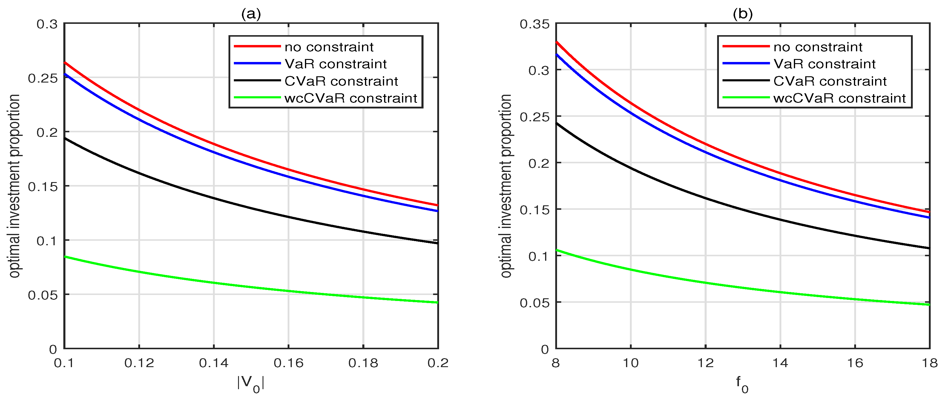
Figure 2 plots the optimal investment strategy without constraints and under dynamic VaR, CVaR and worst-case CVaR constraints. We observe that the optimal investment proportion under dynamic risk measure constraints is lower compared to the scenario without constraints. Among these, the investment proportion is highest under the dynamic VaR constraint and lowest under the dynamic wcCVaR constraint, given that the confidence level remains the same. The introduction of dynamic risk measure constraints restricts managers’ risk exposure to some extent, prompting them to more cautiously control the risk level of their portfolios to avoid potential extreme losses. In addition, from Figure 2b, as the initial wealth $f_0$ increases, the proportion invested in the risky asset relatively decreases. This may reflect that the fund managers tend to adopt a more conservative investment strategy when they have higher initial wealth, reducing the amount of investment in the risky asset to avoid potential financial losses. High initial wealth leads fund managers to focus on preserving value and robust growth, thus decreasing the demand for the risky asset.

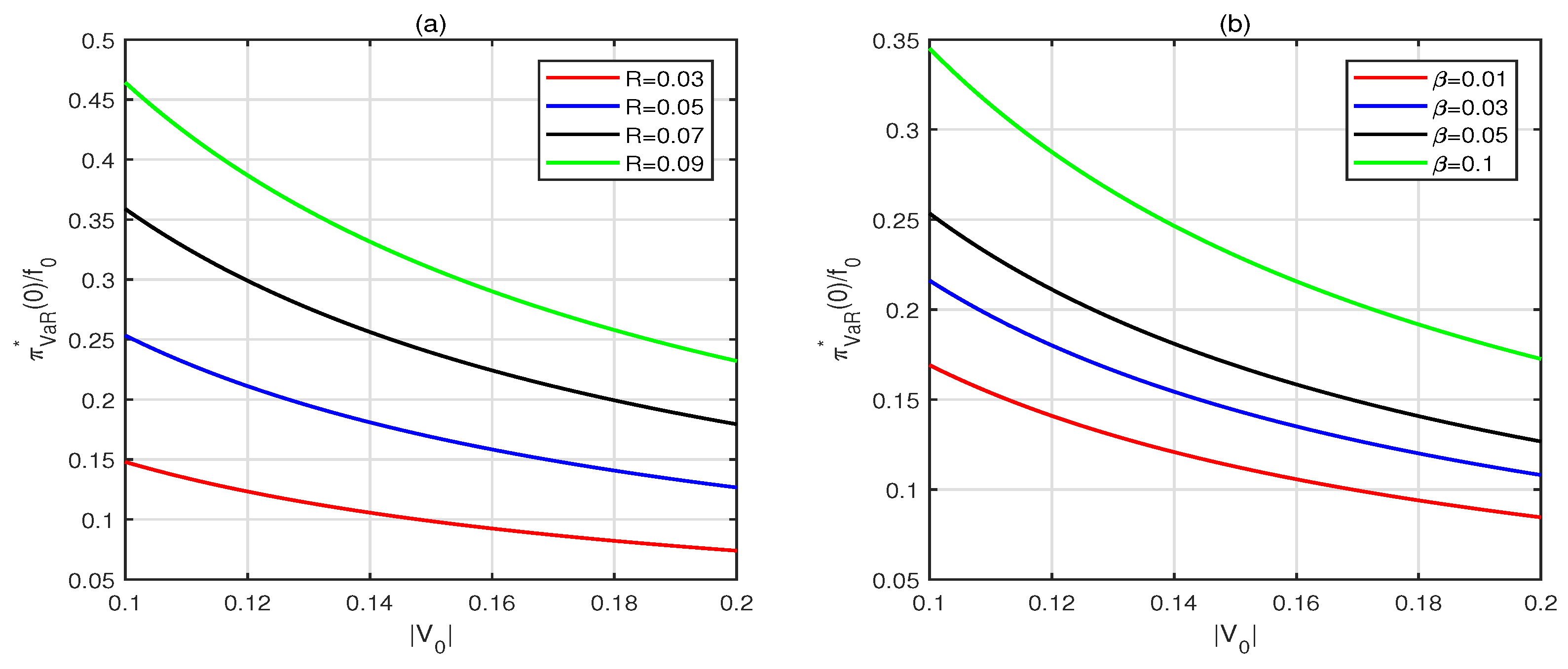
Figure 3a depicts the changes in the optimal investment proportion under different risk levels. It has been observed that as the risk level R increases, the optimal investment proportion also increases. This phenomenon might reflect the notion that fund managers have a higher capacity to bear risk, enabling them to better handle the challenges brought about by risk and uncertainty. With an increase in the risk level, fund managers’ tolerance for extreme losses enhances; thus, they are more inclined to take on greater risks in pursuit of higher returns. This behavior also indicates their confidence in their abilities and investment knowledge, as well as an optimistic view of the market and investment opportunities. Figure 3b shows the optimal investment proportion under dynamic VaR constraint based on different confidence levels. It is found that as $\beta$ decreases, the proportion of investment in the risky asset gradually increases. As the confidence level $1-\beta$ increases, it means that fund managers can maintain investments under a higher potential loss, thereby being more willing to invest in the risky asset. This may be because a lower confidence level reduces sensitivity to asset volatility, allowing for a higher proportion of risk assets in the portfolio in pursuit of higher expected returns.

As the risk premium of the risky asset gradually increases, fund managers often weigh the pursuit of higher returns against taking on greater risks. This trade-off is manifested as an increase in the proportion of the risky asset in the portfolio with the rise of the Sharpe ratio $\xi$. The Sharpe ratio $\xi$ is an important indicator that measures the trade-off between the risk and return of an investment portfolio, helping fund managers to formulate an effective investment strategy. Figure 4a clearly shows this trend, illustrating how the fund managers’ preference for the risky asset gradually strengthens as the risk premium increases. This phenomenon reflects managers’ willingness to bear more risk in the pursuit of higher returns. As shown in Figure 4b, with an increase in pension contribution rate, pension funds usually have more available capital, and thus may consider increasing the allocation proportion of the risky asset to seek higher returns. This trend towards a greater proportion of the risky asset can be seen as a more proactive management approach by pension funds in asset allocation regarding future pension liabilities, while also reflecting the pension funds’ pursuit of long-term investment returns.

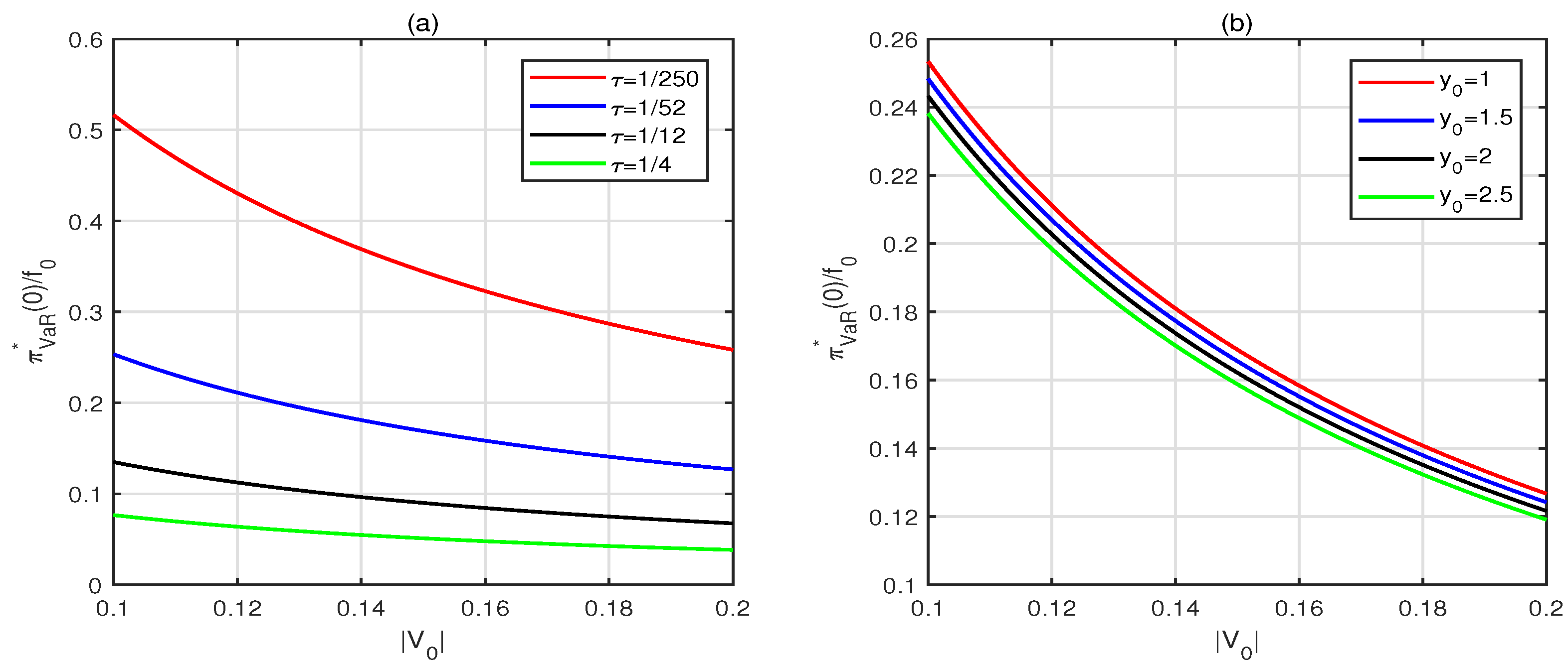
Under the dynamic VaR constraint, the fund manager’s risk reassessment is scheduled at varying frequencies, quarterly, fortnightly, weekly, or daily. Correspondingly, the values of $\tau$ are set as ${\displaystyle \frac{1}{4}}$, ${\displaystyle \frac{1}{25}}$, ${\displaystyle \frac{1}{52}}$, and ${\displaystyle \frac{1}{250}}$. The optimal investment proportions under these different assessment frequencies are depicted in Figure 5a. It is observed that the optimal investment proportion ${\pi }_{\mathrm{VaR}}^{*}\left(0\right)$ shows an upward trend as the interval $\tau$ decreases. A higher level of initial salary typically signifies a greater contribution from an individual or employee to the pension fund, which in turn boosts the total pension fund wealth. As illustrated in Figure 5b, there is a notable trend where the proportion of investments allocated to the risky asset diminishes with an increase in the initial salary level. This indicates a more conservative investment strategy as the pension fund wealth expands.

6. Conclusions

This paper studies the optimal asset allocation problem for a DC pension fund under dynamic VaR, CVaR, and wcCVaR constraints, with a stochastic salary process and a stochastic volatility model. The financial market consists of risk-free and risky assets whose prices are characterized by the Stein–Stein stochastic volatility model. By applying dynamic programming principles and the Lagrange multiplier method, we derive optimal investment strategies both with and without the dynamic VaR constraint.

The results indicate that the optimal investment proportion under dynamic risk measure constraints is lower compared to scenarios without such constraints. Among these, the proportion is highest under the dynamic VaR limit and lowest under the wcCVaR constraint, assuming the same confidence level. Additionally, the confidence level and risk level of the VaR constraint significantly affect the optimal investment strategy. This underscores the necessity of comprehensively considering the VaR constraint to ensure the portfolio can function effectively under various market conditions and achieve long-term asset appreciation goals.

In this paper, we only considered the case where the risk level is constant, which has certain limitations. Risk measures are, in fact, more complex. Therefore, future studies should explore additional risk measures. To better capture the various characteristics of the dynamic VaR, CVaR, and wcCVaR constraints, the upper boundary could be expressed in alternative forms, such as the maximum of a constant value and a percentage of the surplus. Additionally, this paper assumes the Stein–Stein stochastic volatility model. Future research will focus on a broader range of stochastic volatility models.

References

1. Boulier, J.; Huang, S.; Taillard, G. Optimal management under stochastic interest rates: The case of a protected defined contribution pension fund. Insur. Math. Econ. 2001, 28, 173–189. [Google Scholar] [CrossRef]
2. Haberman, S.; Vigna, E. Optimal investment strategies and risk measures in defined contribution pension schemes. Insur. Math. Econ. 2002, 31, 35–69. [Google Scholar] [CrossRef]
3. Cairns, A.; Blake, D.; Dowd, K. Stochastic lifestyling: Optimal dynamic asset allocation for defined contribution pension plans. J. Econ. Dyn. Control 2006, 30, 843–877. [Google Scholar] [CrossRef]
4. Guan, G.; Liang, Z. Mean-variance efficiency of DC pension plan under stochastic interest rate and mean-reverting returns. Insur. Math. Econ. 2015, 61, 99–109. [Google Scholar] [CrossRef]
5. Wu, H.; Zeng, Y. Equilibrium investment strategy for defined-contribution pension schemes with generalized mean-variance criterion and mortality risk. Insur. Math. Econ. 2015, 64, 396–408. [Google Scholar] [CrossRef]
6. Sun, J.; Li, Y.; Zhang, L. Robust portfolio choice for a defined contribution pension plan with stochastic income and interest rate. Commun. Stat.-Theory Methods 2018, 47, 4106–4130. [Google Scholar] [CrossRef]
7. Bian, L.; Li, Z.; Yao, H. Pre-commitment and equilibrium investment strategies for the DC pension plan with regime switching and a return of premiums clause. Insur. Math. Econ. 2018, 81, 78–94. [Google Scholar] [CrossRef]
8. Wang, P.; Shen, Y.; Zhang, L.; Kang, Y. Equilibrium investment strategy for a DC pension plan with learning about stock return predictability. Insur. Math. Econ. 2021, 100, 384–407. [Google Scholar] [CrossRef]
9. Zhang, Y. Optimal DC pension investment with square-root factor processes under stochastic income and inflation risks. Optimization 2023, 72, 2951–2988. [Google Scholar] [CrossRef]
10. Ng, K.; Chong, W. Optimal investment in defined contribution pension schemes with forward utility preferences. Insur. Math. Econ. 2024, 114, 192–211. [Google Scholar] [CrossRef]
11. Guan, G.; Liang, Z. Optimal management of DC pension plan under loss aversion and Value-at-Risk constraints. Insur. Math. Econ. 2016, 69, 224–237. [Google Scholar] [CrossRef]
12. Yan, M.; Cao, Z.; Wang, T.; Zhang, S. Robust optimal investment strategy of DC pension plans with stochastic salary and a return of premiums clause. Commun. Stat.-Theory Methods 2021, 51, 7980–8011. [Google Scholar] [CrossRef]
13. Chang, H.; Li, J.; Zhao, H. Robust optimal strategies of DC pension plans with stochastic volatility and stochastic income under mean-variance criteria. J. Ind. Manag. Optim. 2022, 18, 1393–1423. [Google Scholar] [CrossRef]
14. Gao, J. Optimal portfolios for DC pension plans under a CEV model. Insur. Math. Econ. 2009, 44, 479–490. [Google Scholar] [CrossRef]
15. Wang, Y.; Xu, X.; Zhang, J. Optimal investment strategy for DC pension plan with deposit loan spread under the CEV model. Axioms 2022, 11, 382. [Google Scholar] [CrossRef]
16. Zhao, H.; Rong, X. Portfolio selection problem with multiple risky assets under the constant elasticity of variance model. Insur. Math. Econ. 2012, 50, 179–190. [Google Scholar] [CrossRef]
17. Guan, G.; Liang, Z. Optimal management of DC pension plan in a stochastic interest rate and stochastic volatility framework. Insur. Math. Econ. 2014, 57, 58–66. [Google Scholar] [CrossRef]
18. Ma, J.; Zhao, H.; Rong, X. Optimal investment strategy for a DC pension plan with mispricing under the Heston model. Commun. Stat.-Theory Methods 2020, 49, 3168–3183. [Google Scholar] [CrossRef]
19. He, X.; Zhu, S. An alternative form to calibrate the correlated Stein-Stein option pricing model. Comput. Appl. Math. 2019, 38, 68. [Google Scholar] [CrossRef]
20. Lin, S.; Lin, X.; He, X. Analytically pricing European options with a two-factor Stein-Stein model. J. Comput. Appl. Math. 2024, 440, 115662. [Google Scholar] [CrossRef]
21. Artzner, P.; Delbaen, F.; Eber, J.M.; Heath, D. Coherent measures of risk. Math. Financ. 1999, 9, 203–228. [Google Scholar] [CrossRef]
22. Basak, S.; Shapiro, A. Value-at-risk-based risk management: Optimal policies and asset prices. Rev. Financ. Stud. 2001, 14, 371–405. [Google Scholar] [CrossRef]
23. Čerbáková, J. Worst-case VaR and CVaR. In Operations Research Proceedings; Springer: Berlin/Heidelberg, Germany, 2006; Volume 2005. [Google Scholar]
24. Natarajan, K.; Pachamanova, D.; Sim, M. Constructing risk measures from uncertainty sets. Oper. Res. 2009, 57, 1129–1141. [Google Scholar] [CrossRef]
25. Yiu, K. Optimal portfolios under a value-at-risk constraint. J. Econ. Dyn. Control 2004, 28, 1317–1334. [Google Scholar] [CrossRef]
26. Cuoco, D.; He, H.; Isaenko, S. Optimal dynamic trading strategies with risk limits. Oper. Res. 2008, 56, 358–368. [Google Scholar] [CrossRef]
27. Zhang, N.; Jin, Z.; Li, S.; Chen, P. Optimal reinsurance under dynamic VaR constraint. Insur. Math. Econ. 2016, 71, 232–243. [Google Scholar] [CrossRef]
28. Zhang, Q.; Gao, Y. Portfolio selection based on a benchmark process with dynamic value-at-risk constraints. J. Comput. Appl. Math. 2017, 313, 440–447. [Google Scholar] [CrossRef]
29. Dong, Y.; Tang, C.; Hua, C. Optimal investment of DC pension plan under a joint VaR-ES constraint. AIMS Math. 2024, 9, 2084–2104. [Google Scholar] [CrossRef]
30. Deelstra, G.; Grasselli, M.; Koehl, P.F. Optimal investment strategies in the presence of a minimum guarantee. Insur. Math. Econ. 2003, 33, 189–207. [Google Scholar] [CrossRef]
31. Zhang, C.; Rong, X.; Zhao, H.; Hou, R. Optimal investment for the defined-contribution pension with stochastic salary under a CEV model. Appl. Math.-A J. Chin. Univ. 2013, 28, 187–203. [Google Scholar] [CrossRef]
32. Li, D.; Rong, X.; Zhao, H. Time-consistent investment strategy for DC pension plan with stochastic salary under CEV model. J. Syst. Sci. Complex. 2016, 29, 428–454. [Google Scholar] [CrossRef]
33. Zeng, Y.; Li, D.; Chen, Z.; Yang, Z. Ambiguity aversion and optimal derivative-based pension investment with stochastic income and volatility. J. Econ. Dyn. Control 2018, 88, 70–103. [Google Scholar] [CrossRef]
34. Liu, Z.; Wang, Y.; Huang, Y.; Zhou, J. Optimal portfolios for the DC pension fund with mispricing under the HARA utility framework. J. Ind. Manag. Optim. 2023, 19, 1262–1281. [Google Scholar] [CrossRef]
35. Pirvu, T. Portfolio optimization under the value-at-risk constraint. Quant. Financ. 2007, 7, 125–136. [Google Scholar] [CrossRef]
36. Zhu, S.; Fukushima, M. Worst-case conditional value-at-risk with application to robust portfolio management. Oper. Res. 2009, 57, 1155–1168. [Google Scholar] [CrossRef]
37. Chen, S.; Li, Z.; Li, K. Optimal investment–reinsurance policy for an insurance company with VaR constraint. Insur. Math. Econ. 2010, 47, 144–153. [Google Scholar] [CrossRef]
Figure 1. (a) The effect of | v 0 | and f 0 on the optimal investment strategy π * ( 0 ) / f 0 ; (b) The effect of m on the optimal investment strategy π * ( 0 ) / f 0 .
Axioms 13 00543 g001
Figure 2. (a) The effect of | v 0 | on optimal investment strategies under different constraints; (b) The effect of f 0 on optimal investment strategies under different constraints.
Axioms 13 00543 g002
Figure 3. (a) The effect of R on the optimal investment strategy π VaR * ( 0 ) / f 0 ; (b) The effect of β on the optimal investment strategy π VaR * ( 0 ) / f 0 .
Axioms 13 00543 g003
Figure 4. (a) The effect of ξ on the optimal investment strategy π VaR * ( 0 ) / f 0 ; (b) The effect of p on the optimal investment strategy π VaR * ( 0 ) / f 0 .
Axioms 13 00543 g004
Figure 5. (a) The effect of τ on the optimal investment strategy π VaR * ( 0 ) / f 0 ; (b) The effect of y 0 on the optimal investment strategy π VaR * ( 0 ) / f 0 .
Axioms 13 00543 g005