Well-Posedness of the Schrödinger–Korteweg–de Vries System with Robin Boundary Conditions on the Half-Line

Abstract

The Schrödinger–Korteweg–de Vries (SKdV) system can describe the nonlinear dynamics of phenomena such as Langmuir and ion acoustic waves, which are highly valuable for studying wave behavior and interactions. The SKdV system has wide-ranging applications in physics and applied mathematics. In this article, we investigate the local well-posedness of the SKdV system with Robin boundary conditions and polynomial terms in the Sobolev space. We want to enhance the applicability of this type of SKdV system. Our verification process is as follows: We estimate Fokas solutions for the Robin problem with external forces. Next, we define an iteration map in suitable solution space and prove the iteration map is a contraction mapping and onto some closed ball $B(0,r)$. Finally, by the contraction mapping theorem, we obtain the uniqueness solution. Moreover, we show that the data-to-solution map is locally Lipschitz continuous and conclude with the well-posedness of the SKdV system.

1. Introduction and Main Results

1.1. Introduction

In this article, we study the local well-posedness of the following Schrödinger–Korteweg–de Vries (SKdV) system:

$$\begin{array}{c}\hfill \left\{\begin{array}{cc}i{\partial }_{t}u+{\partial }_x^{2}u=P(u)v,\hfill & x\in (0,\infty ),t\in (0,T),\hfill \\ {\partial }_{t}v+{\partial }_x^{3}v=Q(v)v_x,\hfill & x\in (0,\infty ),t\in (0,T),\hfill \\ u(x,0)=u_0(x)\in H_x^s(0,\infty ),v(x,0)=v_0(x)\in H_x^s(0,\infty ),\hfill & x\in [0,\infty ),\hfill \\ u_x(0,t)-{\gamma }_{1}u(0,t)=g_1(t)\in H_t^{(2s-1)/4}(0,T),\hfill & t\in (0,T),{\gamma }_1\ge 1,\hfill \\ v_x(0,t)-{\gamma }_{2}v(0,t)=g_2(t)\in H_t^{s/3}(0,T),\hfill & t\in (0,T),{\gamma }_2>0,\hfill \end{array}\right.\end{array}$$

where $0<T<1$, $3/4<s<1$, $u(x,t)$ is a complex-valued function, $v(x,t)$ is a real-valued function, and

$$P(u)=\sum _{i=0}^m{a}_i{u}^i\mathrm{and}Q(v)=\sum _{j=0}^n{b}_j{v}^j$$

are polynomials, where $a_i$ and $b_j$ are constants. Well-posedness guarantees the reliability and predictive accuracy of equation models in various fields, making it essential for scientific research, engineering applications, and decision-making. According to our current understanding from studies on the SKdV system, we investigate the local well-posedness of the SKdV system with Robin boundary conditions. We consider the local well-posedness of the SKdV system with Robin boundary conditions from a mathematical point of view. The right side of the equals sign of this system is composed of polynomials mainly because we hope to use polynomials to approximate any arbitrary continuous function, allowing it to be applied to different SKdV systems.

Next, we introduce the SKdV system. The SKdV system is a coupled nonlinear partial differential system consisting of the Schrödinger equation, which describes complex-valued functions, and the Korteweg–de Vries (KdV) equation, which describes real-valued functions. The Schrödinger equation characterizes the temporal evolution of the wave function, while the KdV equation describes the propagation and interaction of nonlinear waves. This system integrates the properties of two types of waves: short waves (described by the Schrödinger equation) and long waves (described by the KdV equation), making it highly applicable to the study of wave phenomena and dynamic behavior.

The SKdV system has wide applications in physics and applied mathematics. In the study of nonlinear waves, the SKdV system can describe the nonlinear dynamics of phenomena such as Langmuir waves and ion acoustic waves, which is very useful for studying wave behavior and interactions [1,2]. In plasma physics, the SKdV system is used to describe wave phenomena in plasmas, such as the interactions between Langmuir waves and ion acoustic waves. This is crucial to understanding the properties and behavior of plasmas [3,4,5,6,7]. In fluid dynamics, the SKdV system is used to study wave phenomena in fluids, such as the nonlinear interactions between short and long waves, and to describe the behavior of water waves under nonlinear and dispersive effects [8,9]. In the field of optics, the SKdV system can be used to describe nonlinear wave and dispersion effects in optical fibers. This helps to understand the propagation characteristics of light in optical fibers and the impact of nonlinear effects on wave behavior [10]. In wave dynamics, the SKdV system is used to describe the propagation and interaction of water waves, which has important applications in oceanography and marine engineering. For example, this system can be used to study the resonant interactions between short and long waves on the water surface [11]. In the control theory of dynamical systems, the SKdV system is used to study the dynamic behavior and control methods of systems [12]. In fractal dynamics, the SKdV system is used to describe dynamical systems with fractal characteristics, and the behavior and properties of such systems are further studied [13,14]. In the study of chaotic synchronization, the SKdV system is used to investigate synchronization phenomena and control methods in chaotic systems [15]. These applications demonstrate the versatile use of the SKdV system in various fields and provide a deep understanding of the dynamic behavior of such systems and control methods.

We present some relatively new research on the SKdV system. Shang, Li, and Li [16] investigate traveling wave solutions of a coupled Schrödinger–Korteweg–de Vries equation using the generalized coupled trial equation method. The researchers have utilized this method to discover a series of exact traveling wave solutions, which hold significant importance in understanding various processes in dusty plasma. This study provides an effective solution for nonlinear evolution equation systems and highlights the practical applications of these equations in physics. Khan, Khan, and Ahmad [17] investigated the fractal fractional nonlinear Korteweg–de-Vries–Schrödinger system with a power law kernel. The study utilizes the Yang transform and Caputo fractional fractal operator, applying the Yang transform homotopy perturbation method to solve this system. The research aims to analyze the existence and uniqueness of the solution and provides graphical representations of the results. The article also involves fixed point theory and nonlinear functional analysis to delve into this challenging mathematical problem. Noor, Alotaibi, Shah, Ismaeel, and El-Tantawy [18] analyze solitary waves and nonlinear oscillations of the fractional Schrödinger–KdV equation using the Caputo Operator framework. They employ the Laplace residual power series method (LRPSM) to study this model and compare the resulting approximations with exact solutions in the integer case. Their research shows that the approximations are highly accurate and more stable over large space-time domains.

Now, we present recent articles that discuss the existence, uniqueness, and well-posedness of solutions associated with the SKdV system. Guo and Miao [6] studied the well-posedness of the Cauchy problem for the SKdV system. By establishing global well-posedness in specific function spaces, this research explored the nonlinear dynamics equations describing one-dimensional Langmuir and ion acoustic waves. The work focused on the mathematical properties of the system, the existence and uniqueness of solutions, and the relationship between the electric field of Langmuir oscillations and low-frequency density perturbations. Corcho and Linares [12] studied the well-posedness of the Cauchy problem for the SKdV system. The authors studied the local well-posedness for weak initial data and obtained well-posedness results for data in Sobolev space $L^2(\mathbb{R})\times H^{-{\displaystyle \frac{3}{4}}+}$. These results also led to global well-posedness in energy space $H^1(\mathbb{R})\times H^1(\mathbb{R})$. The authors improved upon previous research on the well-posedness of the SKdV system. Matheus [19] showed that the Cauchy problem for the SKdV system with periodic functions is globally well-posed in the energy space $H^1\times H^1$. The study used the I-method introduced by Colliander et al. and improved the results of Arbieto et al. on the global well-posedness of the SKdV system. The author conducted a thorough investigation and proof of the global well-posedness of the SKdV system for periodic functions. Guo and Wang [7] studied the well-posedness of the SKdV system, in particular, for initial data in the Sobolev spaces $L^2(\mathbb{R})\times H^{-3/4}(\mathbb{R})$ and $H^s(\mathbb{R})\times H^{-3/4}(\mathbb{R})$ $(s>-1/16)$. The article introduced $F^s$-type spaces to handle the KdV component and coupling terms of the system, overcoming difficulties arising from the lack of scale invariance through unified estimates of multipliers. The authors demonstrated the local well-posedness of the SKdV system for certain initial data under resonance conditions.

Wang and Cui [20] established the local well-posedness of the Cauchy problem for the SKdV system in different function spaces. Using bilinear estimates and other techniques, the authors presented results on the local well-posedness of the system under certain conditions. Guo, Ma, and Zhang [21] investigated the global existence and uniqueness of solutions for the fractional SKdV system. Using the contraction method, the authors addressed local existence and uniqueness and proved the global existence of solutions over time using a priori estimates. Cavalcante and Corcho [10] studied the local progress theory of the SKdV system on the half-line. Cavalcante and Corcho [22] studied the well-posedness and lower bounds of the growth of weighted norms for the SKdV system on the half-line. The authors studied the initial boundary value problem for the SKdV system, analyzing the growth of the weighted norms of the solutions over time. By studying the dynamical properties and norm growth of the SKdV system, they determined the well-posedness and lower bounds, thus gaining a deeper understanding of the behavior and characteristics of this nonlinear evolution system. Chen [23] studied the periodic solutions of the SKdV system, in particular, the influence of boundary and external forces on the solutions. The author discussed the existence of theorems for periodic, quasi-periodic, and nearly periodic solutions, investigating their properties and characteristics under various conditions. The focus was on the stability and periodicity of the solutions, as well as on the influence of external forces on the dynamical behavior of the system. Compaan, Shin, and Tzirakis [24] studied the well-posedness of the SKdV system on the half-line. By applying multilinear harmonic analysis techniques, the authors improved the well-posedness theory based on $L^2$ solutions. They studied the local well-posedness and global existence of the system and proposed theorems describing the behavior of the solutions. In addition, they discussed the smoothing effects and the growth of the solutions under different parameter conditions. Himonas and Yan [11] investigated the well-posedness of the initial boundary value problem for the SKdV system on the half-line. Using the Fokas unified transform method, they analyzed the well-posedness of the problem, discussing linear space-time estimates and quadratic/cubic estimates in Bourgain space.

After introducing the SKdV system, the main research of this paper will be presented next.

1.2. Main Results

In this paper, we demonstrate the local well-posedness of the SKdV system presented below.

$$\begin{array}{c}\hfill \left\{\begin{array}{cc}i{\partial }_{t}u+{\partial }_x^{2}u=P(u)v,\hfill & x\in (0,\infty ),t\in (0,T),\hfill \\ {\partial }_{t}v+{\partial }_x^{3}v=Q(v)v_x,\hfill & x\in (0,\infty ),t\in (0,T),\hfill \\ u(x,0)=u_0(x),v(x,0)=v_0(x),\hfill & x\in [0,\infty ),\hfill \\ u_x(0,t)-{\gamma }_{1}u(0,t)=g_1(t),\hfill & t\in (0,T),{\gamma }_1\ge 1,\hfill \\ v_x(0,t)-{\gamma }_{2}v(0,t)=g_2(t),\hfill & t\in (0,T),{\gamma }_2>0,\hfill \end{array}\right.\end{array}$$

(1)

where $0<T<1$, $u(x,t)$ is a complex-valued function, $v(x,t)$ is a real-valued function,

$$P(u)=\sum _{i=0}^m{a}_i{u}^i\mathrm{and}Q(v)=\sum _{j=0}^n{b}_j{v}^j$$

are polynomials, $a_i$ and $b_j$ are constants, and $u_0(x)\in H_x^s(0,\infty )$ and $v_0(x)\in H_x^s(0,\infty )$ are initial data with $3/4<s<1$. The boundary data $g_1(t)\in H_t^{(2s-1)/4}(0,T)$ and $g_2(t)\in H_t^{s/3}(0,T)$ are suggested by the time regularity of the boundary value problems (BVPs) for the corresponding linear equations.

In this article, we demonstrate the local well-posedness of the initial boundary value problem (IBVP) (1). The proof consists of four steps. In the first step, we replace the nonlinear terms $P(u)v$ and $Q(v)v_x$ with external forces and apply the unified transform method (UTM) to solve the corresponding linear IBVPs. In the second step, we derive linear estimates using the UTM formula, considering data and forcing in suitable spaces. (The UTM and its applications were introduced by Fokas [25,26,27,28]). In the third step, we define an iteration map in a suitable solution space by the UTM formula with the forcing terms replaced by the nonlinearities and prove that the iteration map is a contraction map and onto some closed ball $B(0,r)$, and by the contraction mapping theorem, the IBVP (1) has a unique solution. Finally, in the fourth step, we prove the local Lipschitz continuity of the data-to-solution map, thereby confirming the local well-posedness of the IBVP (1).

In [29], the authors mentioned the advantages of UTM over other standard methods and gave some examples for discussion. The UTM complements the standard method for the following reasons: In situations where the standard method can produce an explicit solution, the UTM can also do so, and the solution formula obtained is equivalent; it is more efficient than the standard method. It is versatile and can generate solution formulas for many problems that cannot be solved by classical methods, especially problems with higher than second-order derivatives; the standard method is a collection of methods for specific equations and boundary conditions, while the UTM uses the same idea. The UTM can generate explicit solution formulas and determine in a straightforward way how many and which boundary conditions lead to a well-formulated problem, especially for problems with higher than second-order derivatives. The solution can be efficiently evaluated by various means, such as parameterization of the integration path, to make the integral easy to evaluate by numerical methods, asymptotic methods like the steep descent method, the residue theorem, etc. Background knowledge is limited to knowledge of Fourier transform and inverse Fourier transform pairs, the residue theorem, and Jordan’s lemma.

Now, we provide an overview of Sobolev spaces. For $s\in \mathbb{R}$, the Sobolev space $H^s(\mathbb{R})$ consists of all tempered distributions F with the finite norm:

$$\begin{array}{c}\hfill {\Vert F\Vert }_{H^s(\mathbb{R})}\doteq {\left({\int }_{\mathbb{R}}{(1+{\xi }^2)}^s{|\widehat{F}(\xi )|}^{2}d\xi \right)}^{{\displaystyle \frac{1}{2}}},\end{array}$$

where the Fourier transform $\widehat{F}(\xi )$ is defined by

$$\begin{array}{c}\hfill \widehat{F}(\xi )\doteq {\int }_{\mathbb{R}}{e}^{-ix\xi }F(x)dx.\end{array}$$

Additionally, for an interval $(a,b)\subset \mathbb{R}$ which may extend to infinity on either side, the Sobolev space $H^s(a,b)$ is defined as

$$\begin{array}{c}\hfill H^s(a,b)=\left\{\begin{array}{c}{f:f=F|}_{(a,b)},\mathrm{where}F\in H^s(\mathbb{R})\hfill \\ {\mathrm{and}\Vert f\Vert }_{H^s(a,b)}\doteq \underset{F\in H^s(\mathbb{R})}{inf}{\Vert F\Vert }_{H^s(\mathbb{R})}<\infty \hfill \end{array}\right\}.\end{array}$$

Solving the forced linear Robin IBVP using the UTM leads us to the following Fourier transform.

Definition 1

(Fourier transform on the half-line). For a test function $\psi (x)$ which is defined on $(0,\infty )$, its half-line Fourier transform is expressed as

$$\begin{array}{c}\hfill \widehat{\psi }(k)\doteq {\int }_0^{\infty }{e}^{-ikx}\psi (x)dx,\end{array}$$

(2)

where $k\in \mathbb{C}$ and $\Im (k)\le 0$. Here, $\Im (k)$ and $\Re (k)$ denote the imaginary and real parts of k, respectively.

Remark 1.

For Equation (2), it is evident that if ψ is an integrable function on $(0,\infty )$, then $\widehat{\psi }(k)$ is well-defined for $\Im (k)\le 0$. In fact, within the more suitable space $L^2(0,\infty )$, the half-line Fourier transform can be defined. Specifically, ψ in $L^2(0,\infty )$ can be extended to the entire real line by defining $\psi (x)=0$ for $x<0$, resulting in a function in $L^2(\mathbb{R})$. Consequently, the half-line Fourier transform of ψ can be expressed using the same formula as the Fourier transform for its extension to the real line. Thus, the inverse of this transform can also be derived, which corresponds to the inverse Fourier transform on the real line.

Let’s start by outlining the first step of our approach to solving the Robin problem related to the forced linear Schrödinger equation and the forced linear KdV equation:

$$\begin{array}{c}\hfill \left\{\begin{array}{cc}i{u}_t+u_{xx}=f_1(x,t),\hfill & x\in (0,\infty ),0<t<T<1,\hfill \\ u(x,0)=u_0(x)\in H_x^s(0,\infty ),\hfill & x\in [0,\infty ),\hfill \\ u_x(0,t)-{\gamma }_{1}u(0,t)=g_1(t)\in H_t^{{\displaystyle \frac{2s-1}{4}}}(0,T),\hfill & 0<t<T<1,{\gamma }_1\ge 1\hfill \end{array}\right.\end{array}$$

(3)

and

$$\begin{array}{c}\hfill \left\{\begin{array}{cc}{v}_t+v_{xxx}=f_2(x,t),\hfill & x\in (0,\infty ),0<t<T<1,\hfill \\ v(x,0)=v_0(x)\in H_x^s(0,\infty ),\hfill & x\in [0,\infty ),\hfill \\ v_x(0,t)-{\gamma }_{2}v(0,t)=g_2(t)\in H_t^{{\displaystyle \frac{s}{3}}}(0,T),\hfill & 0<t<T<1,{\gamma }_2>0,\hfill \end{array}\right.\end{array}$$

(4)

respectively. By the UTM formulation, the solution to (3) is denoted by

$$\begin{array}{cc}\hfill u(x,t)& \doteq S_{LS}[u_0,g_1;f_1](x,t)\hfill \\ \hfill & ={\displaystyle \frac{1}{2\pi }}{\int }_{\mathbb{R}}{e}^{ikx-i{k}^{2}t}\left(\widehat{u_0}(k)-i{\int }_0^t{e}^{i{k}^{2}y}\widehat{f_1}(k,y)dy\right)dk\hfill \\ \hfill & +{\displaystyle \frac{1}{2\pi }}{\int }_{\partial D_1^{+}}{e}^{ikx-i{k}^{2}t}{\displaystyle \frac{k-i{\gamma }_1}{k+i{\gamma }_1}}\left(\widehat{u_0}(-k)-i{\int }_0^t{e}^{i{k}^{2}y}\widehat{f_1}(k,y)dy\right)dk\hfill \\ \hfill & -{\displaystyle \frac{i}{\pi }}{\int }_{\partial D_1^{+}}{e}^{ikx-i{k}^{2}t}{\displaystyle \frac{k}{k+i{\gamma }_1}}\left({\int }_0^t{e}^{i{k}^{2}y}{g}_1(y)dy\right)dk,\hfill \end{array}$$

(5)

where

$$\begin{array}{c}\hfill \widehat{u_0}(k)={\int }_0^{\infty }{e}^{-ikx}{u}_0(x)dx,\Im (k)\le 0,\end{array}$$

and the solution of (4) is denoted by

$$\begin{array}{cc}\hfill v(x,t)& \doteq S_{LK}[v_0,g_2;f_2](x,t)\hfill \\ \hfill & ={\displaystyle \frac{1}{2\pi }}{\int }_{\mathbb{R}}{e}^{ikx+i{k}^{3}t}\left(\widehat{v_0}(k)+F(k,t)\right)dk\hfill \\ \hfill & +{\displaystyle \frac{1}{2\pi }}{\int }_{\partial D_2^{+}}{e}^{ikx+i{k}^{3}t}{\displaystyle \frac{(k-i(\alpha +1){\gamma }_2)\left(F(\alpha k,T)+\widehat{v_0}(\alpha k)\right)}{\alpha (k+i{\gamma }_2)}}dk\hfill \\ \hfill & -{\displaystyle \frac{1}{2\pi }}{\int }_{\partial D_2^{+}}{e}^{ikx+i{k}^{3}t}{\displaystyle \frac{(k(\alpha +1)-i{\gamma }_2)\left(F({\alpha }^{2}k,T)+\widehat{v_0}({\alpha }^{2}k)\right)}{\alpha (k+i{\gamma }_2)}}dk\hfill \\ \hfill & +{\displaystyle \frac{3i}{2\pi }}{\int }_{\partial D_2^{+}}{e}^{ikx+i{k}^{3}t}{\displaystyle \frac{k^2}{k+i{\gamma }_2}}\widetilde{g_2}(k^3,T)dk,\hfill \end{array}$$

(6)

where $\alpha =e^{i2\pi /3}$,

$$\begin{array}{cc}\hfill \widehat{v_0}(k)& ={\int }_0^{\infty }{e}^{-ikx}{v}_0(x)dx,\Im (k)\le 0,\hfill \\ \hfill \widetilde{g_2}(k^3,\tau )& \doteq {\int }_0^{\tau }{e}^{-i{k}^{3}t}{g}_2(t)dt,k\in \mathbb{C},\hfill \\ \hfill F(k,\tau )& \doteq {\int }_0^{\tau }{e}^{-i{k}^{3}t}\widehat{f_2}(k,t)dt={\int }_0^{\tau }{e}^{-i{k}^{3}t}\left({\int }_0^{\infty }{e}^{-ikx}{f}_2(x,t)dx\right)dt,\Im (k)\le 0,\hfill \end{array}$$

and $D_1^{+}$ and $D_2^{+}$ are represented in Figure 1.

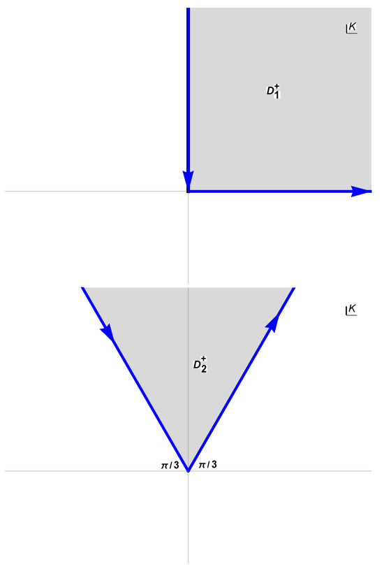
Figure 1. The positively oriented boundaries and regions for $D_1^{+}$ and $D_2^{+}$.

Next, we outline the second step, which involves estimating the Hadamard norm of the UTM solution formulas $S_{LS}[u_0,g_1;f_1]$ (5) and $S_{LK}[v_0,g_2;f_2]$ (6) based on the Sobolev norms of the data and a suitable norm of the forcing. In particular, we have the following linear estimates. The linear estimate for the Schrödinger equation IBVP is as follows:

Theorem 1

(The linear estimate for the Schrödinger equation IBVP [30]). Suppose $1/2<s<3/2$, $u_0(x)\in H_x^s(0,\infty )$, and $g_1(t)\in H_t^{(2s-1)/4}(0,T)$. Then, the solution $u=S_{LS}[u_0,g_1;f_1]\in C\left([0,T];H_x^s(0,\infty )\right)$ of the forced linear Schrödinger equation IBVP (3) given by (5) satisfies the estimate:

$$\begin{array}{c}\underset{t\in [0,T]}{\sup }{\Vert u(t)\Vert }_{H_x^s(0,\infty )}+\underset{x\in [0,\infty )}{\sup }{\Vert u(x)\Vert }_{H_t^{{\displaystyle \frac{2s+1}{4}}}(0,T)}\hfill \\ \le C_s\left(\Vert u_0{\Vert }_{H_x^s(0,\infty )}+\Vert g_1{\Vert }_{H_t^{{\displaystyle \frac{2s-1}{4}}}(0,T)}+\sqrt{T}\underset{t\in [0,T]}{\sup }{\Vert f_1(t)\Vert }_{H_x^s(0,\infty )}\right),\hfill \end{array}$$

(7)

where $C_s=C(s)>0$ is a constant depending on s.

We can use a similar proof process for Theorem 1.2 in [30] to obtain the above theorem.

The linear estimate for the KdV equation IBVP is as follows:

Theorem 2

(The linear estimate for the KdV equation IBVP [31]). Suppose $1/2<s<3/2$, $v_0(x)\in H_x^s(0,\infty )$, and $g_2(t)\in H_t^{s/3}(0,T)$. Then, the solution $v=S_{LK}[v_0,g_2;f_2]\in C\left([0,T];H_x^s(0,\infty )\right)$ of the forced linear KdV equation IBVP (4) given by (6) satisfies the estimate:

$$\begin{array}{c}\underset{t\in [0,T]}{\sup }{\Vert v(t)\Vert }_{H_x^s(0,\infty )}\hfill \\ \le d_s\left(\Vert v_0{\Vert }_{H_x^s(0,\infty )}+{\Vert g_2\Vert }_{H_t^{{\displaystyle \frac{s}{3}}}(0,T)}+T^{{\displaystyle \frac{3-2s}{6}}}{\left({\int }_0^T{\Vert f_2(t)\Vert }_{H_x^s(0,\infty )}^{2}dt\right)}^{{\displaystyle \frac{1}{2}}}\right),\hfill \end{array}$$

(8)

where $d_s=d(s)>0$ is a constant depending on s.

We can find the above theorem in [31].

In the third and fourth steps, our objective is to prove the uniqueness of the solution for (1) and to demonstrate that the data-to-solution map is locally Lipschitz continuous. To achieve this, for $s>1/2$ and $0<T<1$, we define two Banach spaces $X_T$ and $Y_T$:

$$\begin{array}{c}\hfill X_T\doteq C\left([0,T];H_x^s(0,\infty )\right)\cap C\left([0,\infty );H_t^{{\displaystyle \frac{2s+1}{4}}}(0,T)\right)\end{array}$$

with the norm

$$\begin{array}{c}\hfill {\Vert u\Vert }_{X_T}=\underset{t\in [0,T]}{\sup }{\Vert u(t)\Vert }_{H_x^s(0,\infty )}+\underset{x\in [0,\infty )}{\sup }{\Vert u(x)\Vert }_{H_t^{{\displaystyle \frac{2s+1}{4}}}(0,T)}\end{array}$$

(9)

and

$$\begin{array}{c}\hfill Y_T\doteq \left\{\begin{array}{c}v\in C\left([0,T];H_x^s(0,\infty )\right):\hfill \\ {\Vert v\Vert }_{Y_T}\doteq {\Lambda }^T(v)=max\left\{{\Lambda }_{1,s}^T(v),{\Lambda }_{2,s}^T(v),{\Lambda }_3^T(v),{\Lambda }_4^T(v)\right\}<\infty \hfill \end{array}\right\},\end{array}$$

(10)

where the norms ${\Lambda }_{1,s}^T(v),{\Lambda }_{2,s}^T(v),{\Lambda }_3^T(v),{\Lambda }_4^T(v)$ are defined as

$$\begin{array}{c}\hfill {\Lambda }_{1,s}^T(v)=\underset{t\in [0,T]}{\sup }{\Vert v(t)\Vert }_{H_x^s(0,\infty )},{\Lambda }_{2,s}^T(v)={\left(\underset{x\in [0,\infty )}{\sup }{\int }_0^T{\left|D_x^s{\partial }_{x}v(x,t)\right|}^{2}dt\right)}^{{\displaystyle \frac{1}{2}}},\end{array}$$

(11)

$$\begin{array}{c}\hfill {\Lambda }_3^T(v)={\left({\int }_0^{\infty }\underset{t\in [0,T]}{\sup }{\left|v(x,t)\right|}^{2}dx\right)}^{{\displaystyle \frac{1}{2}}},{\Lambda }_4^T(v)={\left({\int }_0^T\underset{x\in [0,\infty )}{\sup }{\left|{\partial }_{x}v(x,t)\right|}^{4}dt\right)}^{{\displaystyle \frac{1}{4}}},\end{array}$$

(12)

where $D_x^s$ is defined by

$$\begin{array}{c}\hfill {\left|D_x^{s}v(x,t)\right|}^2\doteq \left\{\begin{array}{c}{\left|{\partial }_x^{s}v(x,t)\right|}^2,s\in \mathbb{N},\hfill \\ {\int }_0^{\infty }{\displaystyle \frac{{\left|{\partial }_x^{\lfloor s\rfloor }v(x+\zeta ,t)-{\partial }_x^{\lfloor s\rfloor }v(x,t)\right|}^2}{{\zeta }^{1+2\beta }}}d\zeta ,\hfill \end{array}\right.\end{array}$$

where $\lfloor s\rfloor \in {\mathbb{Z}}^{+}\cup \left\{0\right\}$, $s=\lfloor s\rfloor +\beta$, and $0<\beta <1$.

Then, we define the complete metric space ${\mathbb{X}}_T$ and the data space D as

$$\begin{array}{c}\hfill {\mathbb{X}}_T\doteq X_T\times Y_T=\left\{(u,v):u\in X_T,v\in Y_T\right\}\end{array}$$

with the norm

$$\begin{array}{c}\hfill {\Vert (u,v)\Vert }_{{\mathbb{X}}_T}={\Vert u\Vert }_{X_T}+{\Vert v\Vert }_{Y_T}.\end{array}$$

(13)

The data space

$$D=H_x^s(0,\infty )\times H_t^{{\displaystyle \frac{2s-1}{4}}}(0,T)\times H_x^s(0,\infty )\times H_t^{{\displaystyle \frac{s}{3}}}(0,T)$$

with the norm

$$\begin{array}{c}\hfill \Vert (u_0,g_1,v_0,g_2){\Vert }_D=\Vert u_0{\Vert }_{H_x^s(0,\infty )}+\Vert g_1{\Vert }_{H_t^{{\displaystyle \frac{2s-1}{4}}}(0,T)}+\Vert v_0{\Vert }_{H_x^s(0,\infty )}+{\Vert g_2\Vert }_{H_t^{{\displaystyle \frac{s}{3}}}(0,T),}\end{array}$$

(14)

for $(u_0,g_1,v_0,g_2)\in D$.

We then present the main result of this work using the definitions provided above.

Theorem 3

(The local well-posedness of the SKdV system). Consider the SKdV system (1). Suppose $3/4<s<1$ and $0<T<1$. For the data $u_0,v_0\in H_x^s(0,\infty )$, $g_1(t)\in H_t^{(2s-1)/4}(0,T)$, and $g_2(t)\in H_t^{s/3}(0,T)$.

Then, there exist ${\mathfrak{K}}_s=\mathfrak{K}(s)>0$ and ${\tilde{C}}_s=\tilde{C}(s)>0$ which are constants depending on s, and $T^{*}=min\{T,T_1,T_2\}>0$, where

$$\begin{array}{c}\hfill r=max\left\{1,\sqrt{{\displaystyle \frac{3}{2}}}{\widetilde{C_s}}^{-1},2{\mathfrak{K}}_s^{*}{\Vert (u_0,g_1,v_0,g_2)\Vert }_D\right\},\end{array}$$

$$\begin{array}{c}\hfill n_0=max\{m,n\},A=max\{|a_0|,|a_1|,\cdots ,|a_m|\},B=max\{|b_0|,|b_1|\cdots ,|b_n|\},\end{array}$$

$$\begin{array}{c}\hfill T_1={\displaystyle \frac{1}{64{(A(m+1)+\sqrt{10}B)}^6{\left({\mathfrak{K}}_s^{*}\right)}^{6n_0+6}{r}^{6n_0+6}}},\end{array}$$

and

$$\begin{array}{c}\hfill T_2={\displaystyle \frac{1}{64{(A(m^2+m+1)+\sqrt{5}B{\left(2^{n+1}(n+1)+2^n{n}^3\right)}^{\frac{1}{2}})}^6{\left({\mathfrak{K}}_s^{*}\right)}^{6n_0+6}{r}^{6n_0}}},\end{array}$$

such that the SKdV system (1) has a unique solution $(u,v)\in {\mathbb{X}}_{T^{*}}$ and the solution satisfies the size estimate

$$\begin{array}{c}\hfill {\Vert (u,v)\Vert }_{{\mathbb{X}}_{T^{*}}}\le r.\end{array}$$

Furthermore, the data-to-solution map $(u_0,g_1,v_0,g_2)⟼(u,v)$ is locally Lipschitz continuous.

According to the above theorem, we have proven that under certain conditions there will be a unique solution to the SKdV system (1). Regarding the difficulty in studying the local well-posedness of the SKdV system: The SKdV system will involve the algebraic property of the nonlinear estimation term. In two-dimensional space, $H_x^s({\mathbb{R}}^2)$ must be in $s>1$, even in $n\ge 2$ dimensional space, and $H_x^s({\mathbb{R}}^n)$ must be in $s>n/2$ to satisfy the algebraic property. This is a major challenge for existing estimation techniques for the KdV equation.

To facilitate calculations and presentation, we use the following notations.

Remark 2.

For two quantities $\mathcal{A}$ and $\mathcal{B}$ that depend on one or several variables, we write $\mathcal{A}\lesssim \mathcal{B}$ if there exists a positive constant c such that $\mathcal{A}\le c\mathcal{B}$. If $\mathcal{A}\lesssim \mathcal{B}$ and $\mathcal{B}\lesssim \mathcal{A}$, then we denote this relationship by $\mathcal{A}\simeq \mathcal{B}$.

In Section 2, we provide some tools that will be used in later sections. Section 3 outlines the proof of Theorem 2 in preparation for the proof in Section 5. In Section 4 and Section 5, we define a new space, give the $\Lambda$-norm estimates for the UTM solution of the forced linear KdV IBVP (4), and finish the proof of Proposition 2. In Section 6, we define the iteration map and demonstrate that it is a contraction mapping onto a closed ball. We then use the contraction mapping theorem to establish the uniqueness of the solution. Additionally, in Lemma 12, we show that the data-to-solution map is locally Lipschitz continuous. Finally, we complete the proof of Theorem 3.

Regarding Section 6, since we consider the SKdV system with polynomial nonlinear terms, the proof of existence and uniqueness of solutions is more complex than in [30,31,32,33]. In proving that the iteration map is both onto and a contraction, more considerations about the lifetime of the solution are required. For example, the coefficients and degrees of the polynomials affect the length of the existence time, and the size of the unique solution also requires additional considerations based on the data norm and the corresponding range of s. Furthermore, in proving the data-to-solution aspect of local well-posedness, the determination of the lifetime requires more complicated estimates due to the polynomial nonlinear terms in the SKdV system. For example, the existence range of the solution is also affected by the coefficients and degrees of the polynomials. Therefore, the estimates in Section 6 extend and apply the results of [30,31,32,33].

In this paper, we consider the SKdV system with polynomial nonlinear terms and Robin boundary conditions and discuss linear space-time estimates and the polynomial nonlinear terms in Sobolev space. This differs from the work of Himonas and Yan [11], who considered the SKdV system under Dirichlet boundary conditions and discussed linear space-time estimates and quadratic/cubic estimates in Bourgain space.

2. Preliminary Results and Some Useful Tools

This section provides some tools that will be used in later sections.

Lemma 1

([33]). If $r=r_R+i{r}_I$ with $r_I>0$, then

$$\begin{array}{c}\hfill \left|e^{irkx}-e^{irk\zeta }\right|\le \sqrt{2}\left(1+{\displaystyle \frac{|r_R|}{r_I}}\right)\left|e^{-r_{I}kx}-e^{-r_{I}k\zeta }\right|,\forall k,x,\zeta \ge 0.\end{array}$$

Lemma 2

([33]). Suppose $\varphi (k)\in L_k^2(0,\infty )$. Then, the map

$$\varphi (k)⟼{\int }_0^{\infty }{e}^{-ky}\varphi (k)dk$$

is bounded from $L_k^2(0,\infty )$ into $L_y^2(0,\infty )$ with

$$\begin{array}{c}\hfill \Vert {\int }_0^{\infty }{e}^{-ky}{\varphi (k)dk\Vert }_{L_y^2(0,\infty )}\le \sqrt{\pi }{\Vert \varphi (k)\Vert }_{L_k^2(0,\infty )}.\end{array}$$

Lemma 3

([32]). For $m_1<m<m_2$, we have

$$\begin{array}{c}\hfill {\Vert f\Vert }_{H^m}\le {\Vert f\Vert }_{H^{m_1}}^{{\displaystyle \frac{m_2-m}{m_2-m_1}}}{\Vert f\Vert }_{H^{m_2}}^{{\displaystyle \frac{m-m_1}{m_2-m_1}}}.\end{array}$$

Lemma 4

([34]). If $s>n/2$, then $H_x^s({\mathbb{R}}^n)$ is an algebra with respect to the product of functions. That is, if f and g in $H_x^s({\mathbb{R}}^n)$, then $fg\in H_x^s({\mathbb{R}}^n)$ with

$$\begin{array}{c}\hfill {\Vert fg\Vert }_{H_x^s({\mathbb{R}}^n)}\le {(C_1)}_s{\Vert f\Vert }_{H_x^s({\mathbb{R}}^n)}{\Vert g\Vert }_{H_x^s({\mathbb{R}}^n)},\end{array}$$

for some constant ${(C_1)}_s>0$ depending on s.

For the following lemma, we define the following operator

$$\begin{array}{c}\hfill D^r{U}^2(t)R(x)\doteq {\int }_{\mathbb{R}}{e}^{ikx+i{k}^{3}t}{(ik)}^r\widehat{R}(k)dk\simeq {\int }_{\mathbb{R}}{e}^{ikx+i{k}^{3}t}{|k|}^r\widehat{R}(k)dk,\end{array}$$

(15)

where $\widehat{R}(k)$ is the Fourier transform of $R(x)$.

Lemma 5

([31,35,36,37]). For $R\in L_x^2(\mathbb{R})$, the operator $D^{{\displaystyle \frac{1}{4}}}{U}^2(t)R(x)$ defined by (15) is bounded from $L_x^2$ into $L^4[{\mathbb{R}}_t;L_x^{\infty }(0,\infty )]$; that is, it satisfies the estimate

$$\begin{array}{c}\hfill \Vert D^{{\displaystyle \frac{1}{4}}}{U}^2{(t)R(x)\Vert }_{L^4[{\mathbb{R}}_t;L_x^{\infty }(\mathbb{R})]}\le C_T{\Vert R\Vert }_{L_x^2(\mathbb{R})},\end{array}$$

for some constant $C_T>0$.

For the following lemma, we define the operator

$$\begin{array}{c}\hfill {\Delta }^{r}R(x,t)\doteq {\int }_0^{\infty }{e}^{ia{\tau }^{{\displaystyle \frac{1}{3}}}x+i\tau t}{\tau }^r\widehat{R}(\tau )d\tau ,\end{array}$$

(16)

where $\widehat{R}(\tau )$ is the Fourier transform of $R(t)$.

Lemma 6

([35,38]). For $R\in L_t^2(\mathbb{R})$, the operator ${\Delta }^{{\displaystyle \frac{-1}{4}}}R$ defined by (16) is bounded from $L_t^2$ into $L^4[{\mathbb{R}}_t;L_x^{\infty }(0,\infty )]$; that is, it satisfies the estimate

$$\begin{array}{c}\hfill \Vert {\Delta }^{{\displaystyle \frac{-1}{4}}}{R(x,-t)\Vert }_{L^4[{\mathbb{R}}_t;L_x^{\infty }(0,\infty )]}=\Vert {\Delta }^{{\displaystyle \frac{-1}{4}}}{R(x,t)\Vert }_{L^4[{\mathbb{R}}_t;L_x^{\infty }(0,\infty )]}\le C_T{\Vert R\Vert }_{L_t^2(\mathbb{R})},\end{array}$$

for some constant $C_T>0$.

Lemma 7

([32]). If $\mu \in [0,\infty )$, $\beta \in (0,1)\setminus \left\{{\displaystyle \frac{1}{2}}\right\}$, and

$$\begin{array}{c}\hfill \Delta (\mu ,{\displaystyle \frac{1}{\mu }},\beta )\doteq {\int }_0^{\infty }{\int }_0^{\infty }{\displaystyle \frac{\left(e^{-\mu x}-e^{-\mu y}\right)\left(e^{\frac{-x}{\mu }}-e^{\frac{-y}{\mu }}\right)}{{|x-y|}^{1+2\beta }}}dxdy,\end{array}$$

then

$$\begin{array}{c}\hfill \Delta (\mu ,{\displaystyle \frac{1}{\mu }},\beta )={\mathcal{C}}_{\beta }{\left(\mu +{\displaystyle \frac{1}{\mu }}\right)}^{-1}\left({\mu }^{2\beta }+{\left({\displaystyle \frac{1}{\mu }}\right)}^{2\beta }-{\left(\mu +{\displaystyle \frac{1}{\mu }}\right)}^{2\beta }\right),\end{array}$$

where

$$\begin{array}{c}\hfill {\mathcal{C}}_{\beta }=\left\{\begin{array}{cc}{\displaystyle \frac{\Gamma (1-2\beta )}{\beta }},\hfill & \beta \in (0,{\displaystyle \frac{1}{2}}),\hfill \\ {\displaystyle \frac{\pi }{\beta sin(2\pi \beta )\Gamma (2\beta )}},\hfill & \beta \in ({\displaystyle \frac{1}{2}},1),\hfill \end{array}\right.\end{array}$$

and we obtain the estimate

$$\begin{array}{c}\hfill \Delta (\mu ,{\displaystyle \frac{1}{\mu }},\beta )\lesssim {\mathcal{C}}_{\beta }{\left(\mu +{\displaystyle \frac{1}{\mu }}\right)}^{-1},{\mathcal{C}}_{\beta }>0,\beta \in (0,1)\setminus \left\{{\displaystyle \frac{1}{2}}\right\}.\end{array}$$

3. Sketch the Proof of the Theorem 2

This section details the proof of Theorem 2 by breaking down the Robin problem for the forced linear KdV equation into four simpler problems. In Section 3.2, we use Theorems 4 and 5 from Section 3.1 to derive estimates for the IBVPs.

3.1. The Discussion of the Reduced Pure IBVP for the Linear KdV Equation

In this subsection, Theorems 4 and 5 analyze a fundamental Robin problem related to the linear KdV equation and are key tools for estimating the linear IBVPs $(\mathrm{III})$ and $(\mathrm{IV})$ discussed in Section 3.2.

3.1.1. Reduced Pure IBVP

We begin with the most basic linear KdV equation IBVP on the half-line. That is, the homogeneous IBVP with zero initial data and nonzero boundary data.

Furthermore, we assume that the boundary data $g\in H_t^{s/3}(\mathbb{R})$ extends $g_2\in H_t^{s/3}(0,T)$, which is compactly supported in the interval $[0,2]$, and

$$\begin{array}{c}\hfill {\Vert g\Vert }_{H_t^{s/3}(\mathbb{R})}\le 2{\Vert g_2\Vert }_{H_t^{s/3}(0,T)}.\end{array}$$

(17)

This specific problem, referred to as the reduced pure IBVP, can be formulated as follows:

$$\begin{array}{c}\hfill \left\{\begin{array}{cc}{\omega }_t+{\omega }_{xxx}=0\hfill & x\in (0,\infty ),0<t<2,\hfill \\ \omega (x,0)=0,\hfill & x\in [0,\infty ),\hfill \\ {\omega }_x(0,t)-{\gamma }_2\omega (0,t)=g(t)\in H_t^{{\displaystyle \frac{s}{3}}}(\mathbb{R}),\hfill & t\in [0,2],{\gamma }_2>0.\hfill \end{array}\right.\end{array}$$

(18)

According to the UTM formula, the solution to (18) is

$$\begin{array}{cc}\hfill \omega (x,t)=S_{LK}[0,g;0](x,t)& ={\displaystyle \frac{3i}{2\pi }}{\int }_{\partial D_2^{+}}{e}^{ikx+i{k}^{3}t}{\displaystyle \frac{k^2}{k+i{\gamma }_2}}\tilde{g}(k^3,T)dk\hfill \\ \hfill & ={\omega }_1(x,t)+{\omega }_2(x,t).\hfill \end{array}$$

(19)

We use the parameterization $k⟼ak\mathrm{or}{a}^{2}k$, with $a=e^{i\pi /3}$, where

$${\omega }_1(x,t)={\displaystyle \frac{-3i}{2\pi }}{\int }_0^{\infty }{e}^{iakx-i{k}^{3}t}{\displaystyle \frac{k^2}{ak+i{\gamma }_2}}\tilde{g}(-k^3,T)dk,$$

(20)

$${\omega }_2(x,t)={\displaystyle \frac{-3i}{2\pi }}{\int }_0^{\infty }{e}^{i{a}^{2}kx+i{k}^{3}t}{\displaystyle \frac{k^2}{a^{2}k+i{\gamma }_2}}\tilde{g}(k^3,T)dk.$$

(21)

Our objective is to estimate the Hadamard norm of the solution to the IBVP (18). The following theorem, which we found in [31], addresses this estimation.

Theorem 4

(Reduced linear KdV IBVP with Sobolev data [31]). Let $s\ge 0$. For a test function g which is compactly supported in the interval $[0,2]$, the solution (19) to the Robin problem (18) satisfies the estimate

$$\begin{array}{c}\hfill \underset{t\in \mathbb{R}}{\sup }{\Vert \omega (t)\Vert }_{H_x^s(0,\infty )}\le \widetilde{{(C_3)}_s}{\Vert g\Vert }_{H_t^{{\displaystyle \frac{s}{3}}}(\mathbb{R})},\end{array}$$

(22)

where $\widetilde{{(C_3)}_s}$ is a constant depending on s.

3.1.2. Homogeneous IBVP with Zero Initial Data

In this subsection, we consider the pure IBVP:

$$\begin{array}{c}\hfill \left\{\begin{array}{cc}{\tilde{\omega }}_t+{\tilde{\omega }}_{xxx}=0\hfill & x\in (0,\infty ),t\in [0,T],\hfill \\ \tilde{\omega }(x,0)=0,\hfill & x\in [0,\infty ),\hfill \\ {\tilde{\omega }}_x(0,t)-{\gamma }_2\tilde{\omega }(0,t)=g_2(t)\in H_t^{{\displaystyle \frac{s}{3}}}(0,T),\hfill & t\in [0,T],{\gamma }_2>0.\hfill \end{array}\right.\end{array}$$

(23)

We will extend the boundary data $g_2(t)$ from the interval $[0,T]$ to the entire real line $\mathbb{R}$. Our goal is to define a function $g(t)\in H_t^{{\displaystyle \frac{s}{3}}}(\mathbb{R})$ with g compactly supported in the interval $[0,2]$ as an extension of $g_2(t)\in H_t^{{\displaystyle \frac{s}{3}}}(0,T)$. For $1/2<s<3/2$, g is defined by

$$\begin{array}{c}\hfill g(t)=\left\{\begin{array}{cc}{E}_{\theta }(t),\hfill & t\in (0,2),\hfill \\ 0,\hfill & t\in {(0,2)}^c,\hfill \end{array}\right.\end{array}$$

where $\theta \in C_0^{\infty }(\mathbb{R})$ with $|\theta (t)|\le 1$ for all $t\in \mathbb{R}$, $\theta (t)=1$ for all $|t|\le 1$, $\theta (t)=0$ for all $|t|\ge 2$, and $E_{\theta }=\theta (t)E(t)$. Here, $E\in H_t^{{\displaystyle \frac{s}{3}}}(\mathbb{R})$ is an extension of $g_2\in H_t^{{\displaystyle \frac{s}{3}}}(0,T)$ such that

$${\Vert E\Vert }_{H_t^{{\displaystyle \frac{s}{3}}}(\mathbb{R})}\le 2{\Vert g_2\Vert }_{H_t^{{\displaystyle \frac{s}{3}}}(0,T)}.$$

Consequently, we have that g is compactly supported in the interval $[0,2]$ and (17):

$$\begin{array}{c}\hfill {\Vert g\Vert }_{H_t^{{\displaystyle \frac{s}{3}}}(\mathbb{R})}\le 2{\Vert g_2\Vert }_{H_t^{{\displaystyle \frac{s}{3}}}(0,T)},\mathrm{for}{\displaystyle \frac{1}{2}}<s<{\displaystyle \frac{3}{2}}.\end{array}$$

Thus, for IBVP (23), we can derive the following two inequalities: one for space estimates and one for time estimates.

$$\begin{array}{cc}\hfill \underset{t\in [0,T]}{\sup }{\Vert \tilde{\omega }(t)\Vert }_{H_x^s(0,\infty )}& \le \widetilde{{(C_3)}_s}{\Vert g\Vert }_{H_t^{{\displaystyle \frac{s}{3}}}(\mathbb{R})},(\mathrm{by}\mathrm{Theorem}4)\hfill \\ \hfill & \le 2\widetilde{{(C_3)}_s}{\Vert g_2\Vert }_{H_t^{{\displaystyle \frac{s}{3}}}(0,T)},\mathrm{for}{\displaystyle \frac{1}{2}}<s<{\displaystyle \frac{3}{2}},(\mathrm{by}(17)),\hfill \end{array}$$

where $\widetilde{{(C_3)}_s}$ is a constant depending on s.

Therefore, we obtain the following result:

Theorem 5.

For $1/2<s<3/2$ and the boundary data test function $g_2\in H_t^{{\displaystyle \frac{s}{3}}}(0,T)$. The solution for the IBVP (23) which satisfies the following Hadamard space estimate:

$$\begin{array}{c}\hfill \underset{t\in [0,T]}{\sup }\Vert S[0,g_2;0](t){\Vert }_{H_x^s(0,\infty )}\le 2\widetilde{{(C_3)}_s}{\Vert g_2\Vert }_{H_t^{{\displaystyle \frac{s}{3}}}(0,T)},\end{array}$$

where $\widetilde{{(C_3)}_s}$ is a constant depending on s.

3.2. The Norm Estimates of the Forced Linear KdV Equation IBVP (4) (Theorem 2)

In this subsection, we will prove Theorem 2 by breaking down the forced linear KdV equation into four simpler problems.

3.2.1. Decomposition into Simple Problems

To prove Theorem 2, we start by decomposing the forced linear IBVP (4) into a combination of the following problems:

(I)

The homogeneous linear initial value problem (IVP):

$$\begin{array}{c}\hfill \left\{\begin{array}{cc}{V}_t+V_{xxx}=0,\hfill & x\in \mathbb{R},t\in (0,T),\hfill \\ V(x,0)=V_0(x)\in H_x^s(\mathbb{R}),\hfill & x\in \mathbb{R},\hfill \end{array}\right.\end{array}$$

(24)

where $V_0\in H_x^s(\mathbb{R})$ is an extension of the initial datum $v_0\in H_x^s(0,\infty )$ such that

$$\begin{array}{c}\hfill \Vert V_0{\Vert }_{H_x^s(\mathbb{R})}\le 2{\Vert v_0\Vert }_{H_x^s(0,\infty )}\end{array}$$

(25)

with the solution to IVP (24) expressed using the Duhamel formula

$$\begin{array}{c}\hfill V(x,t)=S[V_0;0](x,t)={\displaystyle \frac{1}{2\pi }}{\int }_{\mathbb{R}}{e}^{ikx+i{k}^{3}t}\widehat{V_0}(k)dk,\end{array}$$

(26)

where the Fourier transform with respect to the spatial variable $\widehat{V_0}(\zeta )$ is defined by

$$\begin{array}{c}\hfill \widehat{V_0}(\zeta )={\int }_{\mathbb{R}}{e}^{-i\zeta k}{V}_0(k)dk,\zeta \in \mathbb{R}.\end{array}$$

(II)

The forced linear IVP with zero initial condition:

$$\begin{array}{c}\hfill \left\{\begin{array}{cc}{W}_t^{*}+W_{xxx}^{*}=F_2(x,t),\hfill & x\in \mathbb{R},t\in (0,T),\hfill \\ W^{*}(x,0)=0,\hfill & x\in \mathbb{R},\hfill \end{array}\right.\end{array}$$

(27)

where $F_2(x,t)\in C\left([0,T];H_x^s(\mathbb{R})\right)$ is an extension of $f_2(x,t)\in C\left([0,T];H_x^s(0,\infty )\right)$, which satisfies

$$\begin{array}{c}\hfill \Vert F_2{\Vert }_{L^2\left([0,T];H_x^s(\mathbb{R})\right)}\le 2{\Vert f_2\Vert }_{L^2\left([0,T];H_x^s(0,\infty )\right)}.\end{array}$$

(28)

The solution to IVP (27) is expressed using the Duhamel formula

$$\begin{array}{cc}\hfill W^{*}(x,t)& =S[0;F_2](x,t)={\displaystyle \frac{1}{2\pi }}{\int }_{\mathbb{R}}\left({\int }_0^t{e}^{ikx+i{k}^3(t-t^{\prime })}\widehat{F_2}(k,t^{\prime })d{t}^{\prime }\right)dk\hfill \\ \hfill & ={\int }_0^{t}S[F_2(·,t^{\prime });0](x,t-t^{\prime })d{t}^{\prime }.\hfill \end{array}$$

(29)

(III)

The linear IBVP on the half-line:

$$\begin{array}{c}\hfill \left\{\begin{array}{cc}{v}_t^{\#}+v_{xxx}^{\#}=0\hfill & x\in (0,\infty ),t\in (0,T),\hfill \\ v^{\#}(x,0)=0,\hfill & x\in [0,\infty ),\hfill \\ v_x^{\#}(0,t)-{\gamma }_2{v}^{\#}(0,t)=G_1(t),\hfill & t\in [0,T],{\gamma }_2>0,\hfill \end{array}\right.\end{array}$$

(30)

where $G_1(t)\doteq g_2(t)-V_x(0,t)-W_x^{*}(0,t)$ and $v^{\#}=S[0,G_0;0]$ is the solution of (30).

(IV)

Homogeneous linear IBVP with zero initial condition:

$$\begin{array}{c}\hfill \left\{\begin{array}{cc}{v}_t^{*}+v_{xxx}^{*}=0\hfill & x\in (0,\infty ),t\in (0,T),\hfill \\ v^{*}(x,0)=0,\hfill & x\in [0,\infty ),\hfill \\ v_x^{*}(0,t)-{\gamma }_2{v}^{*}(0,t)=H_1(t),\hfill & t\in [0,T],{\gamma }_2>0,\hfill \end{array}\right.\end{array}$$

(31)

where $H_1(t)\doteq {\gamma }_2(V(0,t)+W^{*}(0,t))$ and $v^{*}=S[0,H_1;0]$ is the solution of (31).

By applying the superposition principle, the UTM solution (6) of the linear IBVP (4) is expressed as follows: for $x>0$ and $0<t<T$,

$$\begin{array}{c}\hfill S_{LK}[v_0,g_2;f_2]={\left.S[V_0;0]\right|}_{x>0}+{\left.S[0;F_2]\right|}_{x>0}+S[0,G_1;0]+S[0,H_1;0],\end{array}$$

(32)

where the four terms on the right-hand side correspond to the solutions of problems (24), (27), (30), and (31), respectively.

3.2.2. The Estimates for the Linear IVPs

We begin by analyzing the components of (32). First, we will estimate the solutions of the homogeneous linear IVP (24) and the forced linear IVP with zero initial condition (27) in Sobolev spaces. The following two theorems from [31] provide the necessary estimates for these IVPs.

Theorem 6

([31]). The function V defined by Formula (26) solves the linear KdV IVP (24) and satisfies the following estimates:

1. 

Space estimate:

$$\begin{array}{c}\hfill \underset{t\in [0,T]}{\sup }{\Vert V(t)\Vert }_{H_x^s(\mathbb{R})}={\Vert V_0\Vert }_{H_x^s(\mathbb{R})},s\in \mathbb{R}.\end{array}$$

(33)

2. 

Time estimates:

$$\begin{array}{cc}\hfill \underset{x\in \mathbb{R}}{\sup }{\Vert V(x)\Vert }_{H_t^{{\displaystyle \frac{s+1}{3}}}(0,T)}& \le {(C_6)}_s{\Vert V_0\Vert }_{H_x^s(\mathbb{R})},s\in \mathbb{R},\hfill \end{array}$$

(34)

$$\begin{array}{cc}\hfill \underset{x\in \mathbb{R}}{\sup }{\Vert V_x(x)\Vert }_{H_t^{{\displaystyle \frac{s}{3}}}(\mathbb{R})}& \le {(C_7)}_s{\Vert V_0\Vert }_{H_x^s(\mathbb{R})},s\in \mathbb{R},\hfill \end{array}$$

(35)

where ${(C_6)}_s$ and ${(C_7)}_s$ are constants depending on s.

Having analyzed the homogeneous linear IVP (24), we now turn to the estimation of the forced linear IVP with zero initial condition (27).

Theorem 7

([31]). The solution $W^{*}=S[0;F_2]$ of the forced linear IVP (27) given by (29) admits the following senses:

1. 

Space estimate:

$$\begin{array}{c}\hfill \underset{t\in [0,T]}{\sup }{\Vert W^{*}(t)\Vert }_{H_x^s(\mathbb{R})}\le {(C_8)}_s{T}^{{\displaystyle \frac{1}{2}}}{\left({\int }_0^T{\Vert F_2(·,t^{\prime })\Vert }_{H_x^s(\mathbb{R})}^{2}d{t}^{\prime }\right)}^{{\displaystyle \frac{1}{2}}},s\in \mathbb{R}.\end{array}$$

(36)

2. 

Time estimates:

$$\begin{array}{cc}\hfill \underset{x\in \mathbb{R}}{\sup }{\Vert W^{*}(x)\Vert }_{H_t^{{\displaystyle \frac{s+1}{3}}}(0,T)}& \le {(C_9)}_s{T}^{{\displaystyle \frac{2-s}{3}}}{\Vert F_2\Vert }_{L^2([0,T];H_x^s(\mathbb{R}))},{\displaystyle \frac{1}{2}}<s<2,\hfill \end{array}$$

(37)

$$\begin{array}{cc}\hfill \underset{x\in \mathbb{R}}{\sup }{\Vert W_x^{*}(x)\Vert }_{H_t^{{\displaystyle \frac{s}{3}}}(0,T)}& \le {(C_{10})}_s{T}^{{\displaystyle \frac{3-2s}{6}}}{\Vert F_2\Vert }_{L^2([0,T];H_x^s(\mathbb{R}))},0\le s<{\displaystyle \frac{3}{2}},\hfill \end{array}$$

(38)

where ${(C_8)}_s$, ${(C_9)}_s$, and ${(C_{10})}_s$ are constants depending on s.

3.2.3. Proof of Theorem 2

In this subsection, we establish Theorem 2 by utilizing Theorems 4–7.

According to Theorem 5, we obtain the following inequality:

$$\underset{t\in [0,T]}{\sup }{\Vert S[0,G_1;0](t)\Vert }_{H_x^s(0,\infty )}\le 2\widetilde{{(C_3)}_s}{\Vert G_1\Vert }_{H_t^{{\displaystyle \frac{s}{3}}}(0,T)},$$

(39)

$$\underset{t\in [0,T]}{\sup }{\Vert S[0,H_1;0](t)\Vert }_{H_x^s(0,\infty )}\le 2\widetilde{{(C_3)}_s}{\Vert H_1\Vert }_{H_t^{{\displaystyle \frac{s}{3}}}(0,T)}.$$

(40)

According to (32), we have the following inequality:

$$\begin{array}{cc}\hfill & \underset{t\in [0,T]}{\sup }{\Vert S_{LK}[v_0,g_2;f_2]\Vert }_{H_x^s(0,\infty )}\hfill \\ \hfill & \le 2\Vert v_0{\Vert }_{H_x^s(0,\infty )}+2{(C_8)}_s{T}^{{\displaystyle \frac{1}{2}}}{\left({\int }_0^T{\Vert f_2(t)\Vert }_{H_x^s(0,\infty )}^{2}dt\right)}^{{\displaystyle \frac{1}{2}}}+2\widetilde{{(C_3)}_s}{\Vert G_1\Vert }_{H_t^{{\displaystyle \frac{s}{3}}}(0,T)}\hfill \\ \hfill & +2\widetilde{{(C_3)}_s}{\Vert H_1\Vert }_{H_t^{{\displaystyle \frac{s}{3}}}(0,T)},(\mathrm{by} (25), (28), (33), (36), (39), (40)).\hfill \end{array}$$

We must estimate $\Vert G_1{\Vert }_{H_t^{{\displaystyle \frac{s}{3}}}(0,T)}$ and $\Vert H_1{\Vert }_{H_t^{{\displaystyle \frac{s}{3}}}(0,T)}$. Then, we obtain the following inequalities:

$$\begin{array}{cc}\hfill \Vert G_1{\Vert }_{H_t^{{\displaystyle \frac{s}{3}}}(0,T)}& =\Vert g_2(t)-V_x(0,t)-W_x^{*}{(0,t)\Vert }_{H_t^{{\displaystyle \frac{s}{3}}}(0,T)}\hfill \\ \hfill & \le \Vert g_2{\Vert }_{H_t^{{\displaystyle \frac{s}{3}}}(0,T)}+\Vert V_x{(0,t)\Vert }_{H_t^{{\displaystyle \frac{s}{3}}}(0,T)}+{\Vert W_x^{*}(0,t)\Vert }_{H_t^{{\displaystyle \frac{s}{3}}}(0,T)}\hfill \\ \hfill & \lesssim \Vert g_2{\Vert }_{H_t^{{\displaystyle \frac{s}{3}}}(0,T)}+\Vert V_0{\Vert }_{H_x^s(\mathbb{R})}+T^{{\displaystyle \frac{3-2s}{6}}}{\Vert F_2\Vert }_{L^2([0,T];H_x^s(\mathbb{R}))},\hfill \\ \hfill & (\mathrm{by}(35)\mathrm{and}(38))\hfill \\ \hfill & \lesssim \Vert g_2{\Vert }_{H_t^{{\displaystyle \frac{s}{3}}}(0,T)}+\Vert v_0{\Vert }_{H_x^s(0,\infty )}+T^{{\displaystyle \frac{3-2s}{6}}}{\Vert f_2\Vert }_{L^2\left([0,T];H_x^s(0,\infty )\right)},\hfill \\ \hfill & (\mathrm{by}(25)\mathrm{and}(28)),\hfill \end{array}$$

(41)

and

$$\begin{array}{cc}\hfill \Vert H_1{\Vert }_{H_t^{{\displaystyle \frac{s}{3}}}(0,T)}& =\Vert {\gamma }_{2}V(0,t)+{\gamma }_2{W}^{*}{(0,t)\Vert }_{H_t^{{\displaystyle \frac{s}{3}}}(0,T)}\hfill \\ \hfill & \le {\gamma }_2{\Vert V(0,t)\Vert }_{H_t^{{\displaystyle \frac{s}{3}}}(0,T)}+{\gamma }_2{\Vert W^{*}(0,t)\Vert }_{H_t^{{\displaystyle \frac{s}{3}}}(0,T)}\hfill \\ \hfill & \le {\gamma }_2{\Vert V(0,t)\Vert }_{H_t^{{\displaystyle \frac{s+1}{3}}}(0,T)}+{\gamma }_2{\Vert W^{*}(0,t)\Vert }_{H_t^{{\displaystyle \frac{s+1}{3}}}(0,T)}\hfill \\ \hfill & \le {(C_6)}_s{\gamma }_2\Vert V_0{\Vert }_{H_x^s(\mathbb{R})}+{(C_9)}_s{\gamma }_2{T}^{{\displaystyle \frac{2-s}{3}}}{\Vert F_2\Vert }_{L^2([0,T];H_x^s(\mathbb{R}))},\hfill \\ \hfill & (\mathrm{by}(34)\mathrm{and}(37))\hfill \\ \hfill & \le 2{(C_6)}_s{\gamma }_2\Vert v_0{\Vert }_{H_x^s(0,\infty )}+2{(C_9)}_s{\gamma }_2{T}^{{\displaystyle \frac{2-s}{3}}}{\Vert f_2\Vert }_{L^2\left([0,T];H_x^s(0,\infty )\right)},\hfill \\ \hfill & (\mathrm{by}(25)\mathrm{and}(28)).\hfill \end{array}$$

(42)

Hence, by (41) and (42), we can yield (8):

$$\begin{array}{cc}\hfill & \underset{t\in [0,T]}{\sup }{\Vert S_{LK}[v_0,g_2;f_2]\Vert }_{H_x^s(0,\infty )}\hfill \\ \hfill & \le d_s\left(\Vert v_0{\Vert }_{H_x^s(0,\infty )}+{\Vert g_2\Vert }_{H_t^{{\displaystyle \frac{s}{3}}}(0,T)}+T^{{\displaystyle \frac{3-2s}{6}}}{\left({\int }_0^T{\Vert f_2(t)\Vert }_{H_x^s(0,\infty )}^{2}dt\right)}^{{\displaystyle \frac{1}{2}}}\right),\hfill \end{array}$$

which concludes this proof of Theorem 2.

4. About the New Solution Space and Some Estimates

One strategy to prove the existence of solutions to our Robin problem for the KdV equation on $(0,\infty )$ is to use (8) with $f_2$ replaced by $Q(v)v_x$. However, the Hadamard space $C([0,T];H_x^s(0,\infty ))$ is not a suitable candidate due to the presence of the term

$${\int }_0^T{\Vert v{v}_x\Vert }_{H_x^s(0,\infty )}^{2}dt.$$

This is precisely the necessary “algebraic property” (refer to Lemma 4).

Hence,

$$\Vert v{v}_x{\Vert }_{H_x^s(0,\infty )}\le {(C_1)}_s{\Vert v\Vert }_{H_x^s(0,\infty )}{\Vert v_x\Vert }_{H_x^s(0,\infty )}$$

for closing the loop is not true. Therefore, we introduce a new solution space, a subspace of the Hadamard space, defined by specific $\Lambda$-norms.

The following lemma was proven in [33]; therefore, we omit its proof here. Below, we provide the bilinear estimate for the problem term.

Lemma 8

(Bilinear estimate on the half-line). For $0\le s<1$ and any u and v in $Y_T$, where the space $Y_T$ is defined in (10), we have the bilinear estimate

$$\begin{array}{cc}\hfill \Vert u{v}_x{\Vert }_{L^2\left([0,T];H_x^s(0,\infty )\right)}^2& \doteq {\int }_0^T{\Vert u{v}_x(t)\Vert }_{H_x^s(0,\infty )}^{2}dt\hfill \\ \hfill & \le T^{{\displaystyle \frac{1}{2}}}{\left({\Lambda }_3^T(u){\Lambda }_4^T(v)\right)}^2+2{\left({\Lambda }_3^T(u){\Lambda }_{2,s}^T(v)\right)}^2+2T^{{\displaystyle \frac{1}{2}}}{\left({\Lambda }_{1,s}^T(u){\Lambda }_4^T(v)\right)}^2.\hfill \end{array}$$

(43)

We now turn to the following useful lemma for our estimation.

Lemma 9.

For $1/2<s<1$ and $0<T<1$, we have the following results:

$$\begin{array}{c}\hfill {\Lambda }_3^T(uv)\le {\Lambda }_{1,s}^T(u){\Lambda }_3^T(v),\end{array}$$

(44)

and

$$\begin{array}{c}\hfill {\Lambda }_{1,s}^T(uv)\le {(C_1)}_s{\Lambda }_{1,s}^T(u){\Lambda }_{1,s}^T(v),\end{array}$$

(45)

for $u,v\in C([0,T];H_x^s(0,\infty ))$, where ${(C_1)}_s$ is a constant depending on s.

Proof. 

By definition of ${\Lambda }_3^T(uv)$,

$$\begin{array}{cc}\hfill {\Lambda }_3^T(uv)& ={\left({\int }_0^{\infty }\underset{t\in [0,T]}{\sup }{\left|u(x,t)v(x,t)\right|}^{2}dx\right)}^{{\displaystyle \frac{1}{2}}}\hfill \\ \hfill & \le {\left({\int }_0^{\infty }\underset{t\in [0,T]}{\sup }\left(\underset{x\in [0,\infty )}{\sup }{\left|u(x,t)\right|}^2\right)\underset{t\in [0,T]}{\sup }{\left|v(x,t)\right|}^{2}dx\right)}^{{\displaystyle \frac{1}{2}}}\hfill \\ \hfill & \le {\left({\int }_0^{\infty }\underset{t\in [0,T]}{\sup }{\Vert u(t)\Vert }_{H_x^s(0,\infty )}^2\underset{t\in [0,T]}{\sup }{\left|v(x,t)\right|}^{2}dx\right)}^{{\displaystyle \frac{1}{2}}},\hfill \\ \hfill & (\mathrm{by}\mathrm{the}\mathrm{Sobolev}\mathrm{Imbedding}\mathrm{Theorem}\mathrm{for}s>1/2)\hfill \\ \hfill & \le \underset{t\in [0,T]}{\sup }{\Vert u(t)\Vert }_{H_x^s(0,\infty )}{\left({\int }_0^{\infty }\underset{t\in [0,T]}{\sup }{\left|v(x,t)\right|}^{2}dx\right)}^{{\displaystyle \frac{1}{2}}},\hfill \\ \hfill & ={\Lambda }_{1,s}^T(u){\Lambda }_3^T(v),\hfill \end{array}$$

we obtain Equation (44).

To estimate ${\Lambda }_{1,s}^T(uv)$:

$$\begin{array}{cc}\hfill {\Lambda }_{1.s}^T(uv)& =\underset{t\in [0,T]}{\sup }{\Vert uv(t)\Vert }_{H_x^s(0,\infty )}\hfill \\ \hfill & \le \underset{t\in [0,T]}{\sup }\left({(C_1)}_s\Vert u(t){\Vert }_{H_x^s(0,\infty )}{\Vert v(t)\Vert }_{H_x^s(0,\infty )}\right),(\mathrm{by}\mathrm{Lemma}4)\hfill \\ \hfill & \le {(C_1)}_s\left(\underset{t\in [0,T]}{\sup }{\Vert u(t)\Vert }_{H_x^s(0,\infty )}\right)\left(\underset{t\in [0,T]}{\sup }{\Vert v(t)\Vert }_{H_x^s(0,\infty )}\right)\hfill \\ \hfill & ={(C_1)}_s{\Lambda }_{1,s}^T(u){\Lambda }_{1,s}^T(v),\hfill \end{array}$$

we obtain Equation (45). □

Finally, we obtain the following proposition.

Proposition 1.

For $1/2<s<1$ and $0<T<1$, we have the following results:

$$\begin{array}{cc}\hfill & {\int }_0^T{\Vert u_1{u}_2\cdots u_n{v}_x(t)\Vert }_{H_x^s(0,\infty )}^{2}dt\hfill \\ \hfill & \le T^{{\displaystyle \frac{1}{2}}}{\left({\Lambda }_{1,s}^T(u_1){\Lambda }_{1,s}^T(u_2)\cdots {\Lambda }_{1,s}^T(u_{n-1}){\Lambda }_3^T(u_n){\Lambda }_4^T(v)\right)}^2\hfill \\ \hfill & +2{\left({\Lambda }_{1,s}^T(u_1){\Lambda }_{1,s}^T(u_2)\cdots {\Lambda }_{1,s}^T(u_{n-1}){\Lambda }_3^T(u_n){\Lambda }_{2,s}^T(v)\right)}^2\hfill \\ \hfill & +2{({(C_1)}_s)}^{2(n-1)}{T}^{{\displaystyle \frac{1}{2}}}{\left({\Lambda }_{1,s}^T(u_1){\Lambda }_{1,s}^T(u_2)\cdots {\Lambda }_{1,s}^T(u_n){\Lambda }_4^T(v)\right)}^2\hfill \\ \hfill & \le 5{\tilde{C}}_s^{2(n-1)}\Vert u_1{\Vert }_{Y_T}^2\Vert u_2{\Vert }_{Y_T}^2\cdots \Vert u_n{\Vert }_{Y_T}^2{\Vert v\Vert }_{Y_T}^2,\hfill \end{array}$$

(46)

where $n\ge 2$, $n\in \mathbb{N}$, and ${\tilde{C}}_s=max\{1,{(C_1)}_s\}$.

Proof. 

We use mathematical induction to prove this lemma.

In the first part, we assume $n=2$. We have

$$\begin{array}{cc}\hfill & {\int }_0^T{\Vert u_1{u}_2{v}_x(t)\Vert }_{H_x^s(0,\infty )}^{2}dt\hfill \\ \hfill & \le T^{{\displaystyle \frac{1}{2}}}{\left({\Lambda }_3^T(u_1{u}_2){\Lambda }_4^T(v)\right)}^2+2{\left({\Lambda }_3^T(u_1{u}_2){\Lambda }_{2,s}^T(v)\right)}^2+2T^{{\displaystyle \frac{1}{2}}}{\left({\Lambda }_{1,s}^T(u_1{u}_2){\Lambda }_4^T(v)\right)}^2,\hfill \\ \hfill & (\mathrm{by}\mathrm{Lemma}8)\hfill \\ \hfill & \le T^{{\displaystyle \frac{1}{2}}}{\left({\Lambda }_{1,s}^T(u_1){\Lambda }_3^T(u_2){\Lambda }_4^T(v)\right)}^2+2{\left({\Lambda }_{1,s}^T(u_1){\Lambda }_3^T(u_2){\Lambda }_{2,s}^T(v)\right)}^2\hfill \\ \hfill & +2T^{{\displaystyle \frac{1}{2}}}{\left({(C_1)}_s{\Lambda }_{1,s}^T(u_1){\Lambda }_{1,s}^T(u_2){\Lambda }_4^T(v)\right)}^2,(\mathrm{by}\mathrm{Lemmas}4\mathrm{and}9)\hfill \\ \hfill & \le 5{\tilde{C}}_s^{2(n-1)}\Vert u_1{\Vert }_{Y_T}^2\Vert u_2{\Vert }_{Y_T}^2{\Vert v\Vert }_{Y_T}^2.\hfill \end{array}$$

Therefore, when $n=2$, the inequality (46) holds.

In the second part, we assume $n=k>2$ and the following inequality

$$\begin{array}{cc}\hfill & {\int }_0^T{\Vert u_1{u}_2\cdots u_k{v}_x(t)\Vert }_{H_x^s(0,\infty )}^{2}dt\hfill \\ \hfill & \le T^{{\displaystyle \frac{1}{2}}}{\left({\Lambda }_{1,s}^T(u_1){\Lambda }_{1,s}^T(u_2)\cdots {\Lambda }_{1,s}^T(u_{k-1}){\Lambda }_3^T(u_k){\Lambda }_4^T(v)\right)}^2\hfill \\ \hfill & +2{\left({\Lambda }_{1,s}^T(u_1){\Lambda }_{1,s}^T(u_2)\cdots {\Lambda }_{1,s}^T(u_{k-1}){\Lambda }_3^T(u_k){\Lambda }_{2,s}^T(v)\right)}^2\hfill \\ \hfill & +2{({(C_1)}_s)}^{2(k-1)}{T}^{{\displaystyle \frac{1}{2}}}{\left({\Lambda }_{1,s}^T(u_1){\Lambda }_{1,s}^T(u_2)\cdots {\Lambda }_{1,s}^T(u_k){\Lambda }_4^T(v)\right)}^2\hfill \\ \hfill & \le 5{\tilde{C}}_s^{2(k-1)}\Vert u_1{\Vert }_{Y_T}^2\Vert u_2{\Vert }_{Y_T}^2\cdots \Vert u_k{\Vert }_{Y_T}^2{\Vert v\Vert }_{Y_T}^2\hfill \end{array}$$

(47)

holds.

Then, when $n=k+1$, we obtain

$$\begin{array}{cc}\hfill & {\int }_0^T{\Vert u_1{u}_2\cdots u_{k+1}{v}_x(t)\Vert }_{H_x^s(0,\infty )}^{2}dt\hfill \\ \hfill & \le T^{{\displaystyle \frac{1}{2}}}{\left({\Lambda }_{1,s}^T(u_1){\Lambda }_{1,s}^T(u_2)\cdots {\Lambda }_{1,s}^T(u_{k-1}){\Lambda }_3^T(u_k{u}_{k+1}){\Lambda }_4^T(v)\right)}^2\hfill \\ \hfill & +2{\left({\Lambda }_{1,s}^T(u_1){\Lambda }_{1,s}^T(u_2)\cdots {\Lambda }_{1,s}^T(u_{k-1}){\Lambda }_3^T(u_k{u}_{k+1}){\Lambda }_{2,s}^T(v)\right)}^2\hfill \\ \hfill & +2{({(C_1)}_s)}^{2(k-1)}{T}^{{\displaystyle \frac{1}{2}}}{\left({\Lambda }_{1,s}^T(u_1){\Lambda }_{1,s}^T(u_2)\cdots {\Lambda }_{1,s}^T(u_{k-1}){\Lambda }_{1,s}^T(u_k{u}_{k+1}){\Lambda }_4^T(v)\right)}^2,\hfill \\ \hfill & (\mathrm{by}\mathrm{Formula}(47))\hfill \\ \hfill & \le T^{{\displaystyle \frac{1}{2}}}{\left({\Lambda }_{1,s}^T(u_1){\Lambda }_{1,s}^T(u_2)\cdots {\Lambda }_{1,s}^T(u_k){\Lambda }_3^T(u_{k+1}){\Lambda }_4^T(v)\right)}^2\hfill \\ \hfill & +2{\left({\Lambda }_{1,s}^T(u_1){\Lambda }_{1,s}^T(u_2)\cdots {\Lambda }_{1,s}^T(u_k){\Lambda }_3^T(u_{k+1}){\Lambda }_{2,s}^T(v)\right)}^2\hfill \\ \hfill & +2{({(C_1)}_s)}^{2(k-1)}{T}^{{\displaystyle \frac{1}{2}}}{\left({\Lambda }_{1,s}^T(u_1){\Lambda }_{1,s}^T(u_2)\cdots {\Lambda }_{1,s}^T(u_{k-1}){(C_1)}_s{\Lambda }_{1,s}^T(u_k){\Lambda }_{1,s}^T(u_{k+1}){\Lambda }_4^T(v)\right)}^2,\hfill \\ \hfill & (\mathrm{by}\mathrm{Lemma}9)\hfill \\ \hfill & \le T^{{\displaystyle \frac{1}{2}}}{\left({\Lambda }_{1,s}^T(u_1){\Lambda }_{1,s}^T(u_2)\cdots {\Lambda }_{1,s}^T(u_k){\Lambda }_3^T(u_{k+1}){\Lambda }_4^T(v)\right)}^2\hfill \\ \hfill & +2{\left({\Lambda }_{1,s}^T(u_1){\Lambda }_{1,s}^T(u_2)\cdots {\Lambda }_{1,s}^T(u_k){\Lambda }_3^T(u_{k+1}){\Lambda }_{2,s}^T(v)\right)}^2\hfill \\ \hfill & +2{({(C_1)}_s)}^{2k}{T}^{{\displaystyle \frac{1}{2}}}{\left({\Lambda }_{1,s}^T(u_1){\Lambda }_{1,s}^T(u_2)\cdots {\Lambda }_{1,s}^T(u_{k-1}){\Lambda }_{1,s}^T(u_k){\Lambda }_{1,s}^T(u_{k+1}){\Lambda }_4^T(v)\right)}^2\hfill \\ \hfill & \le 5{\tilde{C}}_s^{2k}\Vert u_1{\Vert }_{Y_T}^2\Vert u_2{\Vert }_{Y_T}^2\cdots \Vert u_{k+1}{\Vert }_{Y_T}^2{\Vert v\Vert }_{Y_T}^2.\hfill \end{array}$$

Therefore, when $n=k+1$, the inequality (46) holds.

By mathematical induction, we finish the proof of inequality (46). □

Refining our solution space from $C([0,T];H_x^s(0,\infty )$ to $Y_T$ requires additional estimates for the UTM solution $S_{LK}[v_0,g_2;f_2]$ of (4). Therefore, $S_{LK}[v_0,g_2;f_2]$ must be estimated using the $\Lambda$-norms (11) and (12), which define the norm (10) of $Y_T$.

These new linear estimates are presented in the following proposition and are proven in Section 5.

Proposition 2

($\Lambda$-norms estimates for the forced linear IBVP). For $3/4<s<1$, the solution $S_{LK}[v_0,g_2;f_2]$ of the forced linear KdV IBVP (4) defined by the UTM Formula (6) admits the estimate:

$$\begin{array}{cc}\hfill & {\Lambda }^T(S_{LK}[v_0,g_2;f_2])\hfill \\ \hfill & \le {(d_2)}_s\left(\Vert v_0{\Vert }_{H_x^s(o,\infty )}+{\Vert g_2\Vert }_{H_t^{{\displaystyle \frac{s}{3}}}(0,T)}+T^{{\displaystyle \frac{3-2s}{6}}}{\left({\int }_0^T{\Vert f_2(t)\Vert }_{H_x^s(0,\infty )}^{2}dt\right)}^{{\displaystyle \frac{1}{2}}}\right),\hfill \end{array}$$

(48)

where ${(d_2)}_s>0$ is a constant depending on s.

5. The Proof of Proposition 2 (About the Norms Estimates of the Forced Linear KdV IBVP)

In this section, we will prove Proposition 2. Recall that $S_{LK}[v_0,g_2;f_2]$ (32) is the solution of the forced linear KdV IBVP (4),

$$\begin{array}{c}\hfill S_{LK}[v_0,g_2;f_2]={\left.S[V_0;0]\right|}_{x>0}+{\left.S[0;F_2]\right|}_{x>0}+S[0,G_1;0]+S[0,H_1;0],\end{array}$$

where $S[V_0;0]$ is the solution of the linear IVP (24).

$S[0;F_2]$ is the solution of the forced linear IVP (27), and $S[0,G_1;0]$ and $S[0,H_1;0]$ are the solution of the linear IVP (30) and (31), respectively. Now, we must estimate the $\Lambda$-norms for $S_{LK}[v_0,g_2;f_2]$. We decompose the estimate into four cases:

(A)

We estimate the ${\Lambda }_{1,s}^T$-norm for $S_{LK}[v_0,g_2;f_2]$ to obtain

$$\begin{array}{c}\hfill {\Lambda }_{1,s}^T\left(S_{LK}[v_0,g_2;f_2]\right)\lesssim \Vert v_0{\Vert }_{H_x^s(0,\infty )}+{\Vert g_2\Vert }_{H_t^{{\displaystyle \frac{s}{3}}}(0,T)}+T^{{\displaystyle \frac{3-2s}{6}}}{\left({\int }_0^T{\Vert f_2(t)\Vert }_{H_x^s(0,\infty )}^{2}dt\right)}^{{\displaystyle \frac{1}{2}}};\end{array}$$

(49)

(B)

We estimate the ${\Lambda }_{2,s}^T$-norm for $S_{LK}[v_0,g_2;f_2]$ to obtain

$$\begin{array}{c}\hfill {\Lambda }_{2,s}^T\left(S_{LK}[v_0,g_2;f_2]\right)\lesssim \Vert v_0{\Vert }_{H_x^s(o,\infty )}+{\Vert g_2\Vert }_{H_t^{{\displaystyle \frac{s}{3}}}(0,T)}+T^{{\displaystyle \frac{3-2s}{6}}}{\left({\int }_0^T{\Vert f_2(t)\Vert }_{H_x^s(0,\infty )}^{2}dt\right)}^{{\displaystyle \frac{1}{2}}};\end{array}$$

(50)

(C)

When $s>3/4$, we estimate the ${\Lambda }_3^T$-norm for $S_{LK}[v_0,g_2;f_2]$ to obtain

$$\begin{array}{c}\hfill {\Lambda }_3^T\left(S_{LK}[v_0,g_2;f_2]\right)\lesssim \Vert v_0{\Vert }_{H_x^s(o,\infty )}+{\Vert g_2\Vert }_{H_t^{{\displaystyle \frac{s}{3}}}(0,T)}+T^{{\displaystyle \frac{3-2s}{6}}}{\left({\int }_0^T{\Vert f_2(t)\Vert }_{H_x^s(0,\infty )}^{2}dt\right)}^{{\displaystyle \frac{1}{2}}};\end{array}$$

(51)

(D)

We estimate the ${\Lambda }_4^T$-norm for $S_{LK}[v_0,g_2;f_2]$ to obtain

$$\begin{array}{c}\hfill {\Lambda }_4^T\left(S_{LK}[v_0,g_2;f_2]\right)\lesssim \Vert v_0{\Vert }_{H_x^s(o,\infty )}+{\Vert g_2\Vert }_{H_t^{{\displaystyle \frac{s}{3}}}(0,T)}+T^{{\displaystyle \frac{3-2s}{6}}}{\left({\int }_0^T{\Vert f_2(t)\Vert }_{H_x^s(0,\infty )}^{2}dt\right)}^{{\displaystyle \frac{1}{2}}}.\end{array}$$

(52)

Since

$$\begin{array}{cc}\hfill & {\Lambda }^T\left(S_{LK}[v_0,g_2;f_2]\right)\hfill \\ \hfill & =max\left\{{\Lambda }_{1,s}^T\left(S_{LK}[v_0,g_2;f_2]\right),{\Lambda }_{2,s}^T\left(S_{LK}[v_0,g_2;f_2]\right),{\Lambda }_3^T\left(S_{LK}[v_0,g_2;f_2]\right),{\Lambda }_4^T\left(S_{LK}[v_0,g_2;f_2]\right)\right\},\hfill \end{array}$$

and by (49), (50), (51), and (52), we can yield that (48)

$$\begin{array}{cc}\hfill & \Lambda \left(S[v_0,g_2;f_2]\right)\hfill \\ \hfill & \lesssim \Vert v_0{\Vert }_{H_x^s(0,\infty )}+{\Vert g_2\Vert }_{H_t^{{\displaystyle \frac{s}{3}}}(0,T)}+T^{{\displaystyle \frac{3-2s}{6}}}{\left({\int }_0^T{\Vert f_2(t)\Vert }_{H_x^s(0,\infty )}^{2}dt\right)}^{{\displaystyle \frac{1}{2}}},\mathrm{for}{\displaystyle \frac{3}{4}}<s<1.\hfill \end{array}$$

Therefore, the proof of Proposition 2 is complete.

We will now proceed to prove statements $(A)$, $(B)$, $(C)$, and $(D)$.

(A)

The estimate of ${\Lambda }_{1,s}^T$-norm for $S_{LK}[v_0,g_2;f_2]$ is as follows: For $3/4<s<1$,

$$\begin{array}{cc}\hfill & {\Lambda }_{1,s}^T\left(S_{LK}[v_0,g_2;f_2]\right)\hfill \\ \hfill & ={\Lambda }_{1,s}^T\left({\left.S[V_0;0]\right|}_{x>0}+{\left.S[0;F_2]\right|}_{x>0}+S[0,G_1;0]+S[0,H_1;0]\right)\hfill \\ \hfill & \le \underset{t\in [0,T]}{\sup }\Vert {\left.S[V_0;0]\right|}_{x>0}{\Vert }_{H_x^s(0,\infty )}+\underset{t\in [0,T]}{\sup }{\Vert {\left.S[0;F_2]\right|}_{x>0}\Vert }_{H_x^s(0,\infty )}\hfill \\ \hfill & +\underset{t\in [0,T]}{\sup }\Vert S[0,G_1;0]{\Vert }_{H_x^s(0,\infty )}+\underset{t\in [0,T]}{\sup }{\Vert S[0,H_1;0]\Vert }_{H_x^s(0,\infty )}\hfill \\ \hfill & \lesssim \Vert v_0{\Vert }_{H_x^s(0,\infty )}+{\Vert g_2\Vert }_{H_t^{{\displaystyle \frac{s}{3}}}(0,T)}+T^{{\displaystyle \frac{3-2s}{6}}}{\left({\int }_0^T{\Vert f_2(t)\Vert }_{H_x^s(0,\infty )}^{2}dt\right)}^{{\displaystyle \frac{1}{2}}},\hfill \\ \hfill & (\mathrm{by}(25),(28),(33),(36),(39),(40),(41),\mathrm{and}(42).\hfill \end{array}$$

In fact, by (8), we can attain (49).

(B)

The estimate of ${\Lambda }_{2,s}^T$-norm for $S_{LK}[v_0,g_2;f_2]$ is as follows: For $3/4<s<1$,

$$\begin{array}{cc}\hfill & {\Lambda }_{2,s}^T\left(S_{LK}[v_0,g_2;f_2]\right)\hfill \\ \hfill & ={\Lambda }_{2,s}^T\left({\left.S[V_0;0]\right|}_{x>0}+{\left.S[0;F_2]\right|}_{x>0}+S[0,G_1;0]+S[0,H_1;0]\right)\hfill \\ \hfill & ={\left(\underset{x\in [0,\infty )}{\sup }{\int }_0^T{\left|D_x^s{\partial }_x\left({\left.S[V_0;0]\right|}_{x>0}+{\left.S[0;F_2]\right|}_{x>0}+S[0,G_1;0]+S[0,H_1;0]\right)\right|}^{2}dt\right)}^{{\displaystyle \frac{1}{2}}}\hfill \\ \hfill & \lesssim \underset{(a)}{\underbrace{{\left({\sup }_{x\in [0,\infty )}{\int }_0^T{\left|D_x^s{\partial }_{x}S[V_0;0]\right|}^{2}dt\right)}^{{\displaystyle \frac{1}{2}}}}}+\underset{(b)}{\underbrace{{\left({\sup }_{x\in [0,\infty )}{\int }_0^T{\left|D_x^s{\partial }_{x}S[0;F_2]\right|}^{2}dt\right)}^{{\displaystyle \frac{1}{2}}}}}\hfill \\ \hfill & +\underset{(c)}{\underbrace{{\left({\sup }_{x\in [0,\infty )}{\int }_0^T{\left|D_x^s{\partial }_{x}S[0,G_1;0]\right|}^{2}dt\right)}^{{\displaystyle \frac{1}{2}}}}}+\underset{(d)}{\underbrace{{\left({\sup }_{x\in [0,\infty )}{\int }_0^T{\left|D_x^s{\partial }_{x}S[0,H_1;0]\right|}^{2}dt\right)}^{{\displaystyle \frac{1}{2}}}}}.\hfill \end{array}$$

We must estimate $(a)$, $(b)$, $(c)$, and $(d)$; then, we attain the following results:

We estimate $(a)$ as follows:

$$\begin{array}{cc}\hfill (a)& ={\left(\underset{x\in [0,\infty )}{\sup }{\int }_0^T\left|{\int }_0^{\infty }{\displaystyle \frac{{\left|V_x(x+\zeta ,t)-V_x(x,t)\right|}^2}{{\zeta }^{1+2\beta }}}d\zeta \right|dt\right)}^{{\displaystyle \frac{1}{2}}}\hfill \\ \hfill & ={\left(\underset{x\in [0,\infty )}{\sup }{\int }_0^T\left({\int }_0^{\infty }{\displaystyle \frac{{\left|{\int }_{\mathbb{R}}k{e}^{ikx+i{k}^{3}t}\left(e^{ik\zeta }-1\right)\widehat{V_0}(k)dk\right|}^2}{2\pi {\zeta }^{1+2\beta }}}d\zeta \right)dt\right)}^{{\displaystyle \frac{1}{2}}},\hfill \\ \hfill & (\mathrm{let}\eta =k^3\mathrm{and}\mathrm{by}\mathrm{the}\mathrm{Parseval}’\mathrm{s}\mathrm{Theorem})\hfill \\ \hfill & \le {\left(\underset{x\in [0,\infty )}{\sup }{\int }_0^{\infty }\left({\displaystyle \frac{{\int }_{\mathbb{R}}{\left|e^{i{\eta }^{\frac{1}{3}}x}\left(e^{i{\eta }^{\frac{1}{3}}\zeta }-1\right)\frac{\widehat{V_0}({\eta }^{\frac{1}{3}})}{3{\eta }^{\frac{1}{3}}}\right|}^{2}d\eta }{{\zeta }^{1+2\beta }}}\right)d\zeta \right)}^{{\displaystyle \frac{1}{2}}}\hfill \\ \hfill & ={\displaystyle \frac{1}{3}}{\left(\underset{x\in [0,\infty )}{\sup }{\int }_{\mathbb{R}}{\left|{\displaystyle \frac{\widehat{V_0}({\eta }^{\frac{1}{3}})}{3{\eta }^{\frac{1}{3}}}}\right|}^2\left({\int }_0^{\infty }{\displaystyle \frac{{\left|e^{i{\eta }^{\frac{1}{3}}\zeta }-1\right|}^2}{{\zeta }^{1+2\beta }}}d\zeta \right)d\eta \right)}^{{\displaystyle \frac{1}{2}}}\hfill \\ \hfill & ={\displaystyle \frac{1}{3}}{\left(\underset{x\in [0,\infty )}{\sup }{\int }_{\mathbb{R}}{\left|{\displaystyle \frac{\widehat{V_0}({\eta }^{\frac{1}{3}})}{3{\eta }^{\frac{1}{3}}}}\right|}^2\left({\int }_0^{\infty }{\displaystyle \frac{4{sin}^2\left(\frac{{\eta }^{\frac{1}{3}}\zeta }{2}\right)}{{\zeta }^{1+2\beta }}}d\zeta \right)d\eta \right)}^{{\displaystyle \frac{1}{2}}},(\mathrm{let}y={\displaystyle \frac{{\eta }^{\frac{1}{3}}\zeta }{2}})\hfill \\ \hfill & \simeq {\displaystyle \frac{1}{3}}{\left(\underset{x\in [0,\infty )}{\sup }{\int }_{\mathbb{R}}{\left|{\displaystyle \frac{\widehat{V_0}({\eta }^{\frac{1}{3}})}{{\eta }^{\frac{1}{3}}}}\right|}^2{\eta }^{{\displaystyle \frac{2\beta }{3}}}\left({\int }_0^1{\displaystyle \frac{{sin}^{2}y}{y^{1+2\beta }}}dy+\underset{\tau \to \infty }{lim}{\int }_1^{\tau }{\displaystyle \frac{{sin}^{2}y}{y^{1+2\beta }}}dy\right)d\eta \right)}^{{\displaystyle \frac{1}{2}}}\hfill \\ \hfill & \lesssim {\left(\underset{x\in [0,\infty )}{\sup }{\int }_{\mathbb{R}}{\left|{\displaystyle \frac{\widehat{V_0}({\eta }^{\frac{1}{3}})}{{\eta }^{\frac{1}{3}}}}\right|}^2{\eta }^{{\displaystyle \frac{2\beta }{3}}}d\eta \right)}^{{\displaystyle \frac{1}{2}}},(\mathrm{let}\eta =k^3)\hfill \\ \hfill & ={\left({\int }_{\mathbb{R}}3{\left|\widehat{V_0}(k)\right|}^2{k}^{2\beta }dk\right)}^{{\displaystyle \frac{1}{2}}}\le {\left({\int }_{\mathbb{R}}3{\left|\widehat{V_0}(k)\right|}^2{(1+k^2)}^{\beta }dk\right)}^{{\displaystyle \frac{1}{2}}}\lesssim {\Vert V_0\Vert }_{H_x^s(\mathbb{R})}.\hfill \end{array}$$

Therefore, we derive the following inequality:

$$\begin{array}{c}\hfill (a)\lesssim \Vert V_0{\Vert }_{H_x^s(\mathbb{R})}\le 2{\Vert v_0\Vert }_{H_x^s(0,\infty )},(\mathrm{by}(25)).\end{array}$$

(53)

We estimate $(b)$ as follows:

$$\begin{array}{cc}\hfill (b)& ={\left(\underset{x\in [0,\infty )}{\sup }{\int }_0^T{\left|D_x^s{\partial }_{x}S[0;F_2]\right|}^{2}dt\right)}^{{\displaystyle \frac{1}{2}}}\hfill \\ \hfill & ={\left(\underset{x\in [0,\infty )}{\sup }{\int }_0^T{\left|D_x^s{\partial }_x\left({\int }_0^{t}S[F_2(·,t^{\prime });0](x,t-t^{\prime })d{t}^{\prime }\right)\right|}^{2}dt\right)}^{{\displaystyle \frac{1}{2}}}\hfill \\ \hfill & \le {\left(\underset{x\in [0,\infty )}{\sup }{\int }_0^T{\left({\int }_0^t\left|D_x^s{\partial }_{x}S[F_2(·,t^{\prime });0](x,t-t^{\prime })\right|d{t}^{\prime }\right)}^{2}dt\right)}^{{\displaystyle \frac{1}{2}}}\hfill \\ \hfill & \le \underset{x\in [0,\infty )}{\sup }{\int }_0^T{\left({\int }_{t^{\prime }}^T{\left|D_x^s{\partial }_{x}S[F_2(·,t^{\prime });0](x,t-t^{\prime })\right|}^{2}dt\right)}^{{\displaystyle \frac{1}{2}}}d{t}^{\prime }\hfill \\ \hfill & \le \underset{x\in [0,\infty )}{\sup }{\int }_0^T{\left({\int }_0^T{\left|D_x^s{\partial }_{x}S[F_2(·,t^{\prime });0](x,\tau )\right|}^{2}d\tau \right)}^{{\displaystyle \frac{1}{2}}}d{t}^{\prime },(\mathrm{let}\tau =t-t^{\prime })\hfill \\ \hfill & \le {\int }_0^T{\left(\underset{x\in [0,\infty )}{\sup }{\int }_0^T{\left|D_x^s{\partial }_{x}S[F_2(·,t^{\prime });0](x,\tau )\right|}^{2}d\tau \right)}^{{\displaystyle \frac{1}{2}}}d{t}^{\prime }={\int }_0^T{\Lambda }_{2,s}^T\left(S[F_2(·,t^{\prime });0]\right)d{t}^{\prime }\hfill \\ \hfill & \lesssim {\int }_0^T{\Vert F_2(t^{\prime })\Vert }_{H_x^s(\mathbb{R})}d{t}^{\prime },(\mathrm{by}(53))\hfill \\ \hfill & \le T^{{\displaystyle \frac{1}{2}}}{\left({\int }_0^T{\Vert F_2(t^{\prime })\Vert }_{H_x^s(\mathbb{R})}^{2}d{t}^{\prime }\right)}^{{\displaystyle \frac{1}{2}}}\le 2T^{{\displaystyle \frac{1}{2}}}{\left({\int }_0^T{\Vert f_2(t^{\prime })\Vert }_{H_x^s(0,\infty )}^{2}d{t}^{\prime }\right)}^{{\displaystyle \frac{1}{2}}},(\mathrm{by}(28)).\hfill \end{array}$$

Hence, we derive the following inequality:

$$\begin{array}{c}\hfill (b)\lesssim T^{{\displaystyle \frac{1}{2}}}{\left({\int }_0^T{\Vert f_2(t^{\prime })\Vert }_{H_x^s(0,\infty )}^{2}d{t}^{\prime }\right)}^{{\displaystyle \frac{1}{2}}}.\end{array}$$

(54)

To estimate $(c)$ and $(d)$, we consider the UTM solution formula

$$\begin{array}{c}\hfill S_{LK}[0,g;0]={\omega }_1+{\omega }_2,\end{array}$$

(55)

where

$$\begin{array}{c}\hfill {\omega }_1(x,t)={\displaystyle \frac{-3i}{2\pi }}{\int }_0^{\infty }{e}^{iakx-i{k}^{3}t}{\displaystyle \frac{k^2}{ak+i{\gamma }_2}}\tilde{g}(-k^3,T)dk,\\ \hfill {\omega }_2(x,t)={\displaystyle \frac{-3i}{2\pi }}{\int }_0^{\infty }{e}^{i{a}^{2}kx+i{k}^{3}t}{\displaystyle \frac{k^2}{a^{2}k+i{\gamma }_2}}\tilde{g}(k^3,T)dk.\end{array}$$

We assume

$$\begin{array}{c}\hfill {\mathcal{X}}_{[0,T]}=\left\{\begin{array}{cc}1,\hfill & \mathrm{if}x\in [0,T],\hfill \\ 0,\hfill & \mathrm{if}x\in \mathbb{R}\setminus [0,T].\hfill \end{array}\right.\end{array}$$

Now, we estimate ${\Lambda }_{2,s}^T({\omega }_1)$, and the estimate of ${\Lambda }_{2,s}^T({\omega }_2)$ is similar to the estimate of ${\Lambda }_{2,s}^T({\omega }_1)$.

$$\begin{array}{cc}\hfill {\left({\Lambda }_{2,s}^T({\omega }_1)\right)}^2& =\underset{x\in [0,\infty )}{\sup }{\int }_0^T{\left|D_x^s{\partial }_x{\omega }_1(x,t)\right|}^{2}dt\hfill \\ \hfill & =\underset{x\in [0,\infty )}{\sup }{\int }_0^T\left({\int }_0^{\infty }{\displaystyle \frac{{\left|{\partial }_x{\omega }_1(x+\zeta ,t)-{\partial }_x{\omega }_1(x,t)\right|}^2}{{\zeta }^{1+2\beta }}}d\zeta \right)dt\hfill \\ \hfill & \simeq \underset{x\in [0,\infty )}{\sup }{\int }_0^T\left({\int }_0^{\infty }{\displaystyle \frac{{\left|{\int }_0^{\infty }{e}^{iakx-i{k}^{3}t}\left(e^{iak\zeta }-1\right)\frac{k^3}{ak+i{\gamma }_2}\widehat{{\mathcal{X}}_{[0,T]}g}(-k^3)dk\right|}^2}{2\pi {\zeta }^{1+2\beta }}}d\zeta \right)dt\hfill \\ \hfill & \le \underset{x\in [0,\infty )}{\sup }{\int }_0^{\infty }\left({\int }_0^T{\displaystyle \frac{{\left|{\int }_{-\infty }^0{e}^{-ia{\tau }^{\frac{1}{3}}x+i\tau t}\left(e^{-ia{\tau }^{\frac{1}{3}}\zeta }-1\right)\frac{-\tau }{-a{\tau }^{\frac{1}{3}}+i{\gamma }_2}\widehat{{\mathcal{X}}_{[0,T]}g}(\tau )d\tau \right|}^2}{2\pi {\zeta }^{1+2\beta }{|\tau |}^{\frac{2}{3}}}}dt\right)d\zeta ,\hfill \\ \hfill & (\mathrm{by}\mathrm{Fubini}’\mathrm{s}\mathrm{Theorem}\mathrm{and}\mathrm{let}\tau =-k^3)\hfill \\ \hfill & \le \underset{x\in [0,\infty )}{\sup }{\int }_0^{\infty }\left({\displaystyle \frac{{\int }_{-\infty }^0{\left|e^{-ia{\tau }^{\frac{1}{3}}x}\left(e^{-ia{\tau }^{\frac{1}{3}}\zeta }-1\right)\widehat{{\mathcal{X}}_{[0,T]}g}(\tau )\right|}^{2}d\tau }{{\zeta }^{1+2\beta }}}\right)d\zeta ,\hfill \\ \hfill & (\mathrm{by}\mathrm{Parseval}’\mathrm{s}\mathrm{Theorem})\hfill \\ \hfill & \le \underset{x\in [0,\infty )}{\sup }{\int }_0^{\infty }\left({\displaystyle \frac{{\int }_{-\infty }^0{e}^{\sqrt{3}{\tau }^{\frac{1}{3}}x}{\left|e^{\frac{\sqrt{3}}{2}{\tau }^{\frac{1}{3}}\zeta }-1\right|}^2{\left|\widehat{{\mathcal{X}}_{[0,T]}g}(\tau )\right|}^{2}d\tau }{{\zeta }^{1+2\beta }}},\right)d\zeta ,(\mathrm{by}\mathrm{Lemma}1)\hfill \\ \hfill & \le {\int }_0^{\infty }\left({\displaystyle \frac{{\int }_{-\infty }^0{\left|e^{\frac{\sqrt{3}}{2}{\tau }^{\frac{1}{3}}\zeta }-1\right|}^2{\left|\widehat{{\mathcal{X}}_{[0,T]}g}(\tau )\right|}^{2}d\tau }{{\zeta }^{1+2\beta }}}\right)d\zeta \hfill \\ \hfill & ={\int }_{-\infty }^0{\left|\widehat{{\mathcal{X}}_{[0,T]}g}(\tau )\right|}^2\left({\int }_0^{\infty }{\displaystyle \frac{{\left|e^{\frac{\sqrt{3}}{2}{\tau }^{\frac{1}{3}}\zeta }-1\right|}^2}{{\zeta }^{1+2\beta }}}d\zeta \right)d\tau \lesssim {\int }_{-\infty }^0{\left|\widehat{{\mathcal{X}}_{[0,T]}g}(\tau )\right|}^2{\left({\displaystyle \frac{\sqrt{3}}{2}}{\tau }^{{\displaystyle \frac{1}{3}}}\right)}^{2\beta }d\tau ,\hfill \\ \hfill & (\mathrm{let}r=-{\displaystyle \frac{\sqrt{3}}{2}}{\tau }^{{\displaystyle \frac{1}{3}}}\zeta ,\mathrm{and}\mathrm{by}{\int }_0^{\infty }{\displaystyle \frac{{\left(1-e^{-r}\right)}^2}{r^{1+2\beta }}}dr<\infty )\hfill \\ \hfill & \le {\int }_{\mathbb{R}}{\left(1+{\tau }^2\right)}^{{\displaystyle \frac{\beta }{3}}}{\left|\widehat{{\mathcal{X}}_{[0,T]}g}(\tau )\right|}^{2}d\tau =\Vert {\mathcal{X}}_{[0,T]}g{\Vert }_{H_t^{{\displaystyle \frac{\beta }{3}}}(\mathbb{R})}^2\le {\Vert g\Vert }_{H_t^{{\displaystyle \frac{s}{3}}}(\mathbb{R})}^2.\hfill \end{array}$$

We can estimate ${\Lambda }_{2,s}^T({\omega }_2)$ in a similar way. Hence, we obtain the following inequalities:

$$\begin{array}{c}\hfill {\Lambda }_{2,s}^T({\omega }_1)\lesssim {\Vert g\Vert }_{H_t^{{\displaystyle \frac{s}{3}}}(\mathbb{R})},{\Lambda }_{2,s}^T({\omega }_2)\lesssim {\Vert g\Vert }_{H_t^{{\displaystyle \frac{s}{3}}}(\mathbb{R})}.\end{array}$$

(56)

According to (17) and (56), we obtain

$$\begin{array}{c}\hfill {\Lambda }_{2,s}^T\left(S[0,g;0]\right)\lesssim {\Lambda }_{2,s}^T({\omega }_1)+{\Lambda }_{2,s}^T({\omega }_2)\lesssim {\Vert g\Vert }_{H_t^{{\displaystyle \frac{s}{3}}}(\mathbb{R})}\le 2{\Vert g_2\Vert }_{H_t^{{\displaystyle \frac{s}{3}}}(0,T)}.\end{array}$$

(57)

Therefore, we can have the following results:

$$\begin{array}{cc}\hfill (c)& \lesssim \Vert G_1{\Vert }_{H_t^{{\displaystyle \frac{s}{3}}}(0,T)}={\Vert g_2(t)-V_x(0,t)-W_x^{*}(0,t)\Vert }_{H_t^{{\displaystyle \frac{s}{3}}}(0,T)},\hfill \\ \hfill & (\mathrm{by}(17),(30),\mathrm{and}(57))\hfill \\ \hfill & \le \Vert g_2{\Vert }_{H_t^{{\displaystyle \frac{s}{3}}}(0,T)}+\Vert V_x{(0,t)\Vert }_{H_t^{{\displaystyle \frac{s}{3}}}(0,T)}+{\Vert W_x^{*}(0,t)\Vert }_{H_t^{{\displaystyle \frac{s}{3}}}(0,T)}\hfill \\ \hfill & \le \Vert g_2{\Vert }_{H_t^{{\displaystyle \frac{s}{3}}}(0,T)}+{(C_7)}_s\Vert V_0{\Vert }_{H_x^s(\mathbb{R})}+{(C_{10})}_s{T}^{{\displaystyle \frac{3-2s}{6}}}{\Vert F_2\Vert }_{L^2([0,T];H_x^s(\mathbb{R}))},\hfill \\ \hfill & (\mathrm{by}(35)\mathrm{and}(38))\hfill \\ \hfill & \le \Vert g_2{\Vert }_{H_t^{{\displaystyle \frac{s}{3}}}(0,T)}+2{(C_7)}_s\Vert v_0{\Vert }_{H_x^s(0,\infty )}+2{(C_{10})}_s{T}^{{\displaystyle \frac{3-2s}{6}}}{\Vert f_2\Vert }_{L^2\left([0,T];H_x^s(0,\infty )\right)},\hfill \\ \hfill & (\mathrm{by}(25)\mathrm{and}(28))\hfill \\ \hfill & \lesssim \Vert v_0{\Vert }_{H_x^s(o,\infty )}+{\Vert g_2\Vert }_{H_t^{{\displaystyle \frac{s}{3}}}(0,T)}+T^{{\displaystyle \frac{3-2s}{6}}}{\left({\int }_0^T{\Vert f_2(t)\Vert }_{H_x^s(0,\infty )}^{2}dt\right)}^{{\displaystyle \frac{1}{2}}},\hfill \end{array}$$

(58)

and

$$\begin{array}{cc}\hfill (d)& \lesssim \Vert H_1{\Vert }_{H_t^{{\displaystyle \frac{s}{3}}}(0,T)}={\Vert {\gamma }_{2}V(0,t)+{\gamma }_2{W}^{*}(0,t)\Vert }_{H_t^{{\displaystyle \frac{s}{3}}}(0,T)},\hfill \\ \hfill & (\mathrm{by}(17),(31),\mathrm{and}(57))\hfill \\ \hfill & \le |{\gamma }_2{|\Vert V(0,t)\Vert }_{H_t^{{\displaystyle \frac{s}{3}}}(0,T)}+|{\gamma }_2{|\Vert W(0,t)\Vert }_{H_t^{{\displaystyle \frac{s}{3}}}(0,T)}\hfill \\ \hfill & \le |{\gamma }_2{|\Vert V(0,t)\Vert }_{H_t^{{\displaystyle \frac{s+1}{3}}}(0,T)}+|{\gamma }_2{|\Vert W(0,t)\Vert }_{H_t^{{\displaystyle \frac{s+1}{3}}}(0,T)}\hfill \\ \hfill & \le {(C_6)}_s|{\gamma }_2|\Vert V_0{\Vert }_{H_x^s(\mathbb{R})}+{(C_9)}_s|{\gamma }_2|T^{{\displaystyle \frac{2-s}{3}}}{\Vert F_2\Vert }_{L^2([0,T];H_x^s(\mathbb{R}))},\hfill \\ \hfill & (\mathrm{by}(34)\mathrm{and}(37))\hfill \\ \hfill & \le 2{(C_6)}_s|{\gamma }_2|\Vert v_0{\Vert }_{H_x^s(0,\infty )}+2{(C_9)}_s|{\gamma }_2|T^{{\displaystyle \frac{2-s}{3}}}{\Vert f_2\Vert }_{L^2\left([0,T];H_x^s(0,\infty )\right)},\hfill \\ \hfill & (\mathrm{by}(25)\mathrm{and}(28))\hfill \\ \hfill & \lesssim \Vert v_0{\Vert }_{H_x^s(o,\infty )}+T^{{\displaystyle \frac{2-s}{3}}}{\left({\int }_0^T{\Vert f_2(t)\Vert }_{H_x^s(0,\infty )}^{2}dt\right)}^{{\displaystyle \frac{1}{2}}}.\hfill \end{array}$$

(59)

According to (53), (54), (58), and (59), we obtain (50):

$$\begin{array}{cc}\hfill & {\Lambda }_{2,s}^T\left(S_{LK}[v_0,g_2;f_2]\right)\hfill \\ \hfill & \lesssim \Vert v_0{\Vert }_{H_x^s(o,\infty )}+{\Vert g_2\Vert }_{H_t^{{\displaystyle \frac{s}{3}}}(0,T)}+T^{{\displaystyle \frac{3-2s}{6}}}{\left({\int }_0^T{\Vert f_2(t)\Vert }_{H_x^s(0,\infty )}^{2}dt\right)}^{{\displaystyle \frac{1}{2}}}.\hfill \end{array}$$

(C)

The estimate of ${\Lambda }_3^T$-norm for $S_{LK}[v_0,g_2;f_2]$ is as follows: For $3/4<s<1$,

$$\begin{array}{cc}\hfill & {\Lambda }_3^T\left(S_{LK}[v_0,g_2;f_2]\right)\hfill \\ \hfill & ={\left({\int }_0^{\infty }\underset{t\in [0,T]}{\sup }{\left|S_{LK}[v_0,g_2;f_2](x,t)\right|}^{2}dx\right)}^{{\displaystyle \frac{1}{2}}}\hfill \\ \hfill & ={\left({\int }_0^{\infty }\underset{t\in [0,T]}{\sup }{\left|{\left.S[V_0;0]\right|}_{x>0}+{\left.S[0;F_2]\right|}_{x>0}+S[0,G_1;0]+S[0,H_1;0]\right|}^{2}dx\right)}^{{\displaystyle \frac{1}{2}}}\hfill \\ \hfill & \lesssim {\Lambda }_3^T\left(S[V_0;0]\right)+{\Lambda }_3^T\left(S[0;F_2]\right)+{\Lambda }_3^T\left(S[0,G_1;0]\right)+{\Lambda }_3^T\left(S[0,H_1;0]\right).\hfill \end{array}$$

We must estimate ${\Lambda }_3^T\left(S[V_0;0]\right)$, ${\Lambda }_3^T\left(S[0;F_2]\right)$, ${\Lambda }_3^T\left(S[0,G_1;0]\right)$, and ${\Lambda }_3^T\left(S[0,H_1;0]\right)$.

The estimate of ${\Lambda }_3^T\left(S[V_0;0]\right)$ according to (25) in [37] is

$$\begin{array}{c}\hfill {\Lambda }_3^T\left(S[V_0;0]\right)\le {(C_{14})}_s{(1+T)}^{\rho }{\Vert v_0\Vert }_{H_x^s(0,\infty )},\mathrm{for}s,\rho >{\displaystyle \frac{3}{4}}.\end{array}$$

(60)

The estimate of ${\Lambda }_3^T\left(S_{LK}[0;F_2]\right)$ is as follows:

$$\begin{array}{cc}\hfill & {\Lambda }_3^T\left(S_{LK}[0;F_2]\right)\hfill \\ \hfill & ={\left({\int }_0^{\infty }\underset{t\in [0,T]}{\sup }{\left|{\int }_0^t{S}_{LK}[F_2(·,t^{\prime });0](x,t-t^{\prime })d{t}^{\prime }\right|}^{2}dx\right)}^{{\displaystyle \frac{1}{2}}},\hfill \\ \hfill & (\sin \mathrm{ce}\left|S_{LK}[F_2(·,t^{\prime });0](x,t-t^{\prime })\right|\le {\sup }_{\tau \in [0,T]}\left|S_{LK}[F_2(·,t^{\prime });0](x,\tau )\right|,0\le t^{\prime }\le t\le T,x\in [0,\infty ),\hfill \\ \hfill & \mathrm{and}\mathrm{let}\tau =t-t^{\prime }),\hfill \\ \hfill & \le {\left({\int }_0^{\infty }{\left|{\int }_0^T\underset{\tau \in [0,T]}{\sup }\left|S_{LK}[F_2(·,t^{\prime });0](x,\tau )\right|d{t}^{\prime }\right|}^{2}dx\right)}^{{\displaystyle \frac{1}{2}}}\hfill \\ \hfill & \le {\int }_0^T{\left({\int }_0^{\infty }\underset{\tau \in [0,T]}{\sup }{\left|S_{LK}[F_2(·,t^{\prime });0](x,\tau )\right|}^{2}dx\right)}^{{\displaystyle \frac{1}{2}}}d{t}^{\prime }\hfill \\ \hfill & ={\int }_0^T{\Lambda }_3^T\left(S_{LK}[F_2(·,t^{\prime });0]\right)d{t}^{\prime }\hfill \\ \hfill & \lesssim {\int }_0^T{(1+T)}^{\rho }{\Vert f_2(t^{\prime })\Vert }_{H_x^s(0,\infty )}d{t}^{\prime },(\mathrm{by}(60))\hfill \\ \hfill & \lesssim {(1+T)}^{\rho }{T}^{{\displaystyle \frac{1}{2}}}{\left({\int }_0^T{\Vert f_2(t)\Vert }_{H_x^s(0,\infty )}^{2}dt\right)}^{{\displaystyle \frac{1}{2}}},\mathrm{for}s,\rho >{\displaystyle \frac{3}{4}}.\hfill \end{array}$$

(61)

The estimates of ${\Lambda }_3^T\left(S_{LK}[0,G_1;0]\right)$ and ${\Lambda }_3^T\left(S_{LK}[0,H_1;0]\right)$ are as follows: We consider the UTM solution Formula (55) and

$$\begin{array}{cc}\hfill {\Lambda }_3^T\left(S_{LK}[0,g;0]\right)& ={\Lambda }_3^T\left({\omega }_1+{\omega }_2\right)\hfill \\ \hfill & \le \sqrt{2}{\left({\int }_0^{\infty }\underset{t\in [0,T]}{\sup }{\left|{\omega }_1(x,t)\right|}^{2}dx\right)}^{{\displaystyle \frac{1}{2}}}+\sqrt{2}{\left({\int }_0^{\infty }\underset{t\in [0,T]}{\sup }{\left|{\omega }_2(x,t)\right|}^{2}dx\right)}^{{\displaystyle \frac{1}{2}}}\hfill \\ \hfill & =\sqrt{2}{\Lambda }_3^T\left({\omega }_1\right)+\sqrt{2}{\Lambda }_3^T\left({\omega }_2\right).\hfill \end{array}$$

We will estimate ${\Lambda }_3^T\left({\omega }_1\right)$, noting that the estimate for ${\Lambda }_3^T\left({\omega }_2\right)$ follows similarly to that of ${\Lambda }_3^T\left({\omega }_1\right)$.

$$\begin{array}{cc}\hfill {\Lambda }_3^T\left({\omega }_1\right)& ={\left({\int }_0^{\infty }\underset{t\in [0,T]}{\sup }{\left|{\omega }_1(x,t)\right|}^{2}dx\right)}^{{\displaystyle \frac{1}{2}}}\hfill \\ \hfill & \le {\left({\int }_0^{\infty }\underset{t\in [0,T]}{\sup }{\left({\int }_0^{\infty }{e}^{-{\displaystyle \frac{\sqrt{3}}{2}}kx}k\left|\widehat{{\mathcal{X}}_{[0,T]}g}(-k^3)\right|dk\right)}^{2}dx\right)}^{{\displaystyle \frac{1}{2}}}\hfill \\ \hfill & ={\left({\int }_0^{\infty }\underset{t\in [0,T]}{\sup }{\left({\int }_0^{\infty }{e}^{-ky}k\left|\widehat{{\mathcal{X}}_{[0,T]}g}(-k^3)\right|dk\right)}^2{\displaystyle \frac{2}{\sqrt{3}}}dy\right)}^{{\displaystyle \frac{1}{2}}},(\mathrm{let}y={\displaystyle \frac{\sqrt{3}}{2}}x)\hfill \\ \hfill & \lesssim {\left({\int }_0^{\infty }{k}^2{\left|\widehat{{\mathcal{X}}_{[0,T]}g}(-k^3)\right|}^{2}dk\right)}^{{\displaystyle \frac{1}{2}}},(\mathrm{by}\mathrm{Lemma}2)\hfill \\ \hfill & \le {\left({\int }_{\mathbb{R}}{\left|\widehat{{\mathcal{X}}_{[0,T]}g}(\eta )\right|}^{2}d\eta \right)}^{{\displaystyle \frac{1}{2}}},(\mathrm{let}\eta =-k^3)\hfill \\ \hfill & =\Vert {\mathcal{X}}_{[0,T]}g{\Vert }_{L^2(\mathbb{R})}\le {\Vert g\Vert }_{H_t^{{\displaystyle \frac{s}{3}}}(\mathbb{R})}.\hfill \end{array}$$

We can estimate ${\Lambda }_3^T\left({\omega }_2\right)$ in the same way. Hence, we obtain the following inequalities:

$$\begin{array}{c}\hfill {\Lambda }_3^T\left({\omega }_1\right)\lesssim {\Vert g\Vert }_{H_t^{{\displaystyle \frac{s}{3}}}(\mathbb{R})},{\Lambda }_3^T\left({\omega }_2\right)\lesssim {\Vert g\Vert }_{H_t^{{\displaystyle \frac{s}{3}}}(\mathbb{R})}.\end{array}$$

Hence, we can yield that

$$\begin{array}{c}\hfill {\Lambda }_3^T\left(S_{LK}[0,g;0]\right)\lesssim {\Vert g\Vert }_{H_t^{{\displaystyle \frac{s}{3}}}(\mathbb{R})}\le 2{\Vert g_2\Vert }_{H_t^{{\displaystyle \frac{s}{3}}}(0,T)},(\mathrm{by}(17)).\end{array}$$

(62)

Therefore, we can have the following results:

$$\begin{array}{cc}\hfill & {\Lambda }_3^T\left(S[0,G_1;0]\right)\hfill \\ \hfill & \lesssim \Vert G_1{\Vert }_{H_t^{{\displaystyle \frac{s}{3}}}(0,T)}={\Vert g_2(t)-V_x(0,t)-W_x^{*}(0,t)\Vert }_{H_t^{{\displaystyle \frac{s}{3}}}(0,T)},\hfill \\ \hfill & (\mathrm{by}(17),(18),(30),\mathrm{and}(62))\hfill \\ \hfill & \le \Vert g_2{\Vert }_{H_t^{{\displaystyle \frac{s}{3}}}(0,T)}+\Vert V_x{(0,t)\Vert }_{H_t^{{\displaystyle \frac{s}{3}}}(0,T)}+{\Vert W_x^{*}(0,t)\Vert }_{H_t^{{\displaystyle \frac{s}{3}}}(0,T)}\hfill \\ \hfill & \le \Vert g_2{\Vert }_{H_t^{{\displaystyle \frac{s}{3}}}(0,T)}+{(C_7)}_s\Vert V_0{\Vert }_{H_x^s(\mathbb{R})}+{(C_{10})}_s{T}^{{\displaystyle \frac{3-2s}{6}}}{\Vert F_2\Vert }_{L^2([0,T];H_x^s(\mathbb{R}))},\hfill \\ \hfill & (\mathrm{by}(35)\mathrm{and}(38))\hfill \\ \hfill & \le \Vert g_2{\Vert }_{H_t^{{\displaystyle \frac{s}{3}}}(0,T)}+2{(C_7)}_s\Vert v_0{\Vert }_{H_x^s(0,\infty )}+2{(C_{10})}_s{T}^{{\displaystyle \frac{3-2s}{6}}}{\Vert f_2\Vert }_{L^2\left([0,T];H_x^s(0,\infty )\right)},\hfill \\ \hfill & (\mathrm{by}(25)\mathrm{and}(28))\hfill \\ \hfill & \lesssim \Vert v_0{\Vert }_{H_x^s(o,\infty )}+{\Vert g_2\Vert }_{H_t^{{\displaystyle \frac{s}{3}}}(0,T)}+T^{{\displaystyle \frac{3-2s}{6}}}{\left({\int }_0^T{\Vert f_2(t)\Vert }_{H_x^s(0,\infty )}^{2}dt\right)}^{{\displaystyle \frac{1}{2}}},\hfill \end{array}$$

(63)

and

$$\begin{array}{cc}\hfill {\Lambda }_3^T\left(S[0,H_1;0]\right)& \lesssim \Vert H_1{\Vert }_{H_t^{{\displaystyle \frac{s}{3}}}(0,T)}={\Vert {\gamma }_{2}V(0,t)+{\gamma }_2{W}^{*}(0,t)\Vert }_{H_t^{{\displaystyle \frac{s}{3}}}(0,T)},\hfill \\ \hfill & (\mathrm{by}(17),(18),(30),\mathrm{and}(62))\hfill \\ \hfill & \le |{\gamma }_2{|\Vert V(0,t)\Vert }_{H_t^{{\displaystyle \frac{s}{3}}}(0,T)}+|{\gamma }_2|\Vert W^{*}{(0,t)\Vert }_{H_t^{{\displaystyle \frac{s}{3}}}(0,T)}\hfill \\ \hfill & \le |{\gamma }_2{|\Vert V(0,t)\Vert }_{H_t^{{\displaystyle \frac{s+1}{3}}}(0,T)}+|{\gamma }_2|\Vert W^{*}{(0,t)\Vert }_{H_t^{{\displaystyle \frac{s+1}{3}}}(0,T)}\hfill \\ \hfill & \le {(C_6)}_s|{\gamma }_2|\Vert V_0{\Vert }_{H_x^s(\mathbb{R})}+{(C_9)}_s|{\gamma }_2|T^{{\displaystyle \frac{2-s}{3}}}{\Vert F_2\Vert }_{L^2([0,T];H_x^s(\mathbb{R}))},\hfill \\ \hfill & (\mathrm{by}(34)\mathrm{and}(37))\hfill \\ \hfill & \le 2{(C_6)}_s|{\gamma }_2|\Vert v_0{\Vert }_{H_x^s(0,\infty )}+2{(C_9)}_s|{\gamma }_2|T^{{\displaystyle \frac{2-s}{3}}}{\Vert f_2\Vert }_{L^2\left([0,T];H_x^s(0,\infty )\right)},\hfill \\ \hfill & (\mathrm{by}(25)\mathrm{and}(28))\hfill \\ \hfill & \lesssim \Vert v_0{\Vert }_{H_x^s(o,\infty )}+T^{{\displaystyle \frac{2-s}{3}}}{\left({\int }_0^T{\Vert f_2(t)\Vert }_{H_x^s(0,\infty )}^{2}dt\right)}^{{\displaystyle \frac{1}{2}}}.\hfill \end{array}$$

(64)

According to (60), (61), (63), and (64), we obtain (51):

$$\begin{array}{cc}\hfill & {\Lambda }_3^T\left(S_{LK}[v_0,g_2;f_2]\right)\hfill \\ \hfill & \lesssim \Vert v_0{\Vert }_{H_x^s(o,\infty )}+{\Vert g_2\Vert }_{H_t^{{\displaystyle \frac{s}{3}}}(0,T)}+T^{{\displaystyle \frac{3-2s}{6}}}{\left({\int }_0^T{\Vert f_2(t)\Vert }_{H_x^s(0,\infty )}^{2}dt\right)}^{{\displaystyle \frac{1}{2}}},\mathrm{for}s>{\displaystyle \frac{3}{4}}.\hfill \end{array}$$

(D)

The estimate of ${\Lambda }_4^T$-norm for $S_{LK}[v_0,g_2;f_2]$ is as follows: For $3/4<s<1$,

$$\begin{array}{cc}\hfill & {\Lambda }_4^T\left(S_{LK}[v_0,g_2;f_2]\right)\hfill \\ \hfill & ={\left({\int }_0^T\underset{x\in [0,\infty )}{\sup }{\left|{\partial }_x{S}_{LK}[v_0,g_2;f_2](x,t)\right|}^{4}dt\right)}^{{\displaystyle \frac{1}{4}}}\hfill \\ \hfill & ={\left({\int }_0^T\underset{x\in [0,\infty )}{\sup }{\left|{\left.{\partial }_{x}S[V_0;0]\right|}_{x>0}+{\left.{\partial }_{x}S[0;F_2]\right|}_{x>0}+{\partial }_{x}S[0,G_1;0]+{\partial }_{x}S[0,H_1;0]\right|}^{4}dt\right)}^{{\displaystyle \frac{1}{4}}}\hfill \\ \hfill & \lesssim {\left({\int }_0^T\underset{x\in [0,\infty )}{\sup }{\left({\left|{\partial }_{x}S[V_0;0]\right|}^2+{\left|{\partial }_{x}S[0;F_2]\right|}^2+{\left|{\partial }_{x}S[0,G_1;0]\right|}^2+{\left|{\partial }_{x}S[0,H_1;0]\right|}^2\right)}^{2}dt\right)}^{{\displaystyle \frac{1}{4}}}\hfill \\ \hfill & \lesssim {\Lambda }_4^T\left(S[V_0;0]\right)+{\Lambda }_4^T\left(S[0;F_2]\right)+{\Lambda }_4^T\left(S[0,G_1;0]\right)+{\Lambda }_4^T\left(S[0,H_1;0]\right).\hfill \end{array}$$

We must estimate ${\Lambda }_4^T\left(S[V_0;0]\right)$, ${\Lambda }_4^T\left(S[0;F_2]\right)$, ${\Lambda }_4^T\left(S[0,G_1;0]\right)$, and ${\Lambda }_4^T\left(S[0,H_1;0]\right)$.

The estimate of ${\Lambda }_4^T\left(S_{LK}[V_0;0]\right)$ is as follows: we define the operator

$$\begin{array}{c}\hfill D^r{U}^2(t)R(x)\doteq {\int }_{\mathbb{R}}{e}^{ikx+i{k}^{3}t}{(ik)}^r\widehat{R}(k)dk\simeq {\int }_{\mathbb{R}}{e}^{ikx+i{k}^{3}t}{|k|}^r\widehat{R}(k)dk,\end{array}$$

where $\widehat{R}(k)$ denotes the Fourier transform of $R(x)$.

Now, we apply Lemma 5 to estimate ${\Lambda }_4^T\left(S_{LK}[V_0;0]\right)$:

$$\begin{array}{cc}\hfill {\Lambda }_4^T\left(S_{LK}[V_0;0]\right)& ={\left({\int }_0^T\underset{x\in [0,\infty )}{\sup }{\left|{\partial }_{x}V(x,t)\right|}^{4}dt\right)}^{{\displaystyle \frac{1}{4}}}\hfill \\ \hfill & ={\left({\int }_0^T\underset{x\in [0,\infty )}{\sup }{\left|{\displaystyle \frac{1}{2\pi }}{\int }_{\mathbb{R}}ik{e}^{ikx+i{k}^{3}t}\widehat{V_0}(k)dk\right|}^{4}dt\right)}^{{\displaystyle \frac{1}{4}}},\hfill \\ \hfill & (\mathrm{let}R(x)={\displaystyle \frac{1}{2\pi }}{\int }_{\mathbb{R}}{e}^{ikx}\widehat{R}(k)dk\mathrm{and}\widehat{R}(k)=k^{{\displaystyle \frac{3}{4}}}\widehat{V_0}(k))\hfill \\ \hfill & ={\left({\int }_0^T\underset{x\in [0,\infty )}{\sup }{\left|{\displaystyle \frac{1}{2\pi }}{D}^{{\displaystyle \frac{1}{4}}}{U}^2(t)R(x)\right|}^{4}dt\right)}^{{\displaystyle \frac{1}{4}}}\hfill \\ \hfill & \le {\left({\int }_0^T{\Vert D^{{\displaystyle \frac{1}{4}}}{U}^2(t)R(x)\Vert }_{L_x^{\infty }(\mathbb{R})}^{4}dt\right)}^{{\displaystyle \frac{1}{4}}}\hfill \\ \hfill & \le \Vert D^{{\displaystyle \frac{1}{4}}}{U}^2{(t)R(x)\Vert }_{L^4[{\mathbb{R}}_t;L_x^{\infty }(\mathbb{R})]}\lesssim {\Vert R\Vert }_{L_x^2(\mathbb{R})},(\mathrm{by}\mathrm{Lemma}5)\hfill \\ \hfill & ={\left({\int }_{\mathbb{R}}{\left|R(x)\right|}^{2}dx\right)}^{{\displaystyle \frac{1}{2}}}={\left({\int }_{\mathbb{R}}{|\widehat{R}(k)|}^{2}dk\right)}^{{\displaystyle \frac{1}{2}}}\hfill \\ \hfill & \le {\left({\int }_{\mathbb{R}}{\left(1+k^2\right)}^{{\displaystyle \frac{3}{4}}}{\left|\widehat{V_0}(k)\right|}^{2}dk\right)}^{{\displaystyle \frac{1}{2}}}=\Vert V_0{\Vert }_{H_x^{{\displaystyle \frac{3}{4}}}(\mathbb{R})}\le 2{\Vert v_0\Vert }_{H_x^s(0,\infty )},\mathrm{for}s\ge {\displaystyle \frac{3}{4}}.\hfill \end{array}$$

(65)

Hence, we can yield that

$$\begin{array}{c}\hfill {\Lambda }_4^T\left(S_{LK}[V_0;0]\right)\lesssim 2{\Vert v_0\Vert }_{H_x^s(0,\infty )},\mathrm{for}s\ge {\displaystyle \frac{3}{4}}.\end{array}$$

(66)

The estimate of ${\Lambda }_4^T\left(S_{LK}[0;F_2]\right)$ is as follows:

$$\begin{array}{cc}\hfill & {\Lambda }_4^T\left(S_{LK}[0;F_2]\right)\hfill \\ \hfill & ={\left({\int }_0^T\underset{x\in [0,\infty )}{\sup }{\left|{\partial }_x{S}_{LK}[0;F_2](x,t)\right|}^{4}dt\right)}^{{\displaystyle \frac{1}{4}}}\hfill \\ \hfill & \le {\left({\int }_0^T{\left({\int }_0^t\underset{x\in [0,\infty )}{\sup }\left|{\partial }_x{S}_{LK}[F_2(·,t^{\prime });0](x,t-t^{\prime })\right|d{t}^{\prime }\right)}^{4}dt\right)}^{{\displaystyle \frac{1}{4}}},\hfill \\ \hfill & \le {\int }_0^T{\left({\int }_{t^{\prime }}^T\underset{x\in [0,\infty )}{\sup }{\left|{\partial }_x{S}_{LK}[F_2(·,t^{\prime });0](x,t-t^{\prime })\right|}^{4}dt\right)}^{{\displaystyle \frac{1}{4}}}d{t}^{\prime },\hfill \\ \hfill & (\mathrm{by}\mathrm{Minkowski}’\mathrm{s}\mathrm{integral}\mathrm{inequality})\hfill \\ \hfill & \le {\int }_0^T{\left({\int }_0^T\underset{x\in [0,\infty )}{\sup }{\left|{\partial }_x{S}_{LK}[F_2(·,t^{\prime });0](x,\tau )\right|}^{4}d\tau \right)}^{{\displaystyle \frac{1}{4}}}d{t}^{\prime }\hfill \\ \hfill & (\mathrm{let}\tau =t-t^{\prime })\hfill \\ \hfill & ={\int }_0^T{\Lambda }_4^T\left(S_{LK}[F_2(·,t^{\prime });0]\right)d{t}^{\prime }\lesssim {\int }_0^T{\Vert f_2(t^{\prime })\Vert }_{H_x^s(0,\infty )}d{t}^{\prime },(\mathrm{by}(65))\hfill \\ \hfill & \le T^{{\displaystyle \frac{1}{2}}}{\left({\int }_0^T{\Vert f_2(t^{\prime })\Vert }_{H_x^s(0,\infty )}^{2}d{t}^{\prime }\right)}^2,(\mathrm{by}\mathrm{the}\mathrm{Cauchy}\text{–}\mathrm{Schwartz}\mathrm{inequality}).\hfill \end{array}$$

Hence, we can yield that

$$\begin{array}{c}\hfill {\Lambda }_4^T\left(S_{LK}[0;F_2]\right)\lesssim T^{{\displaystyle \frac{1}{2}}}{\left({\int }_0^T{\Vert f_2(t^{\prime })\Vert }_{H_x^s(0,\infty )}^{2}d{t}^{\prime }\right)}^2.\end{array}$$

The estimate of ${\Lambda }_4^T\left(S_{LK}[0,G_1;0]\right)$ and ${\Lambda }_4^T\left(S_{LK}[0,H_1;0]\right)$ are as follows: According to the UTM solution Formula (55) and

$$\begin{array}{cc}\hfill {\Lambda }_4^T\left(S[0,g;0]\right)& ={\Lambda }_4^T\left({\omega }_1+{\omega }_2\right)\hfill \\ \hfill & \lesssim {\left({\int }_0^T\underset{t\in [0,T]}{\sup }{\left|{\partial }_x{\omega }_1(x,t)\right|}^{4}dx\right)}^{{\displaystyle \frac{1}{4}}}+{\left({\int }_0^T\underset{t\in [0,T]}{\sup }{\left|{\partial }_x{\omega }_2(x,t)\right|}^{4}dx\right)}^{{\displaystyle \frac{1}{4}}}\hfill \\ \hfill & ={\Lambda }_4^T\left({\omega }_1\right)+{\Lambda }_4^T\left({\omega }_2\right).\hfill \end{array}$$

We will estimate ${\Lambda }_4^T\left({\omega }_1\right)$, noting that the estimate for ${\Lambda }_4^T\left({\omega }_2\right)$ follows similarly to that of ${\Lambda }_4^T\left({\omega }_1\right)$.

$$\begin{array}{cc}\hfill {\Lambda }_4^T\left({\omega }_1\right)& ={\left({\int }_0^T\underset{x\in [0,\infty )}{\sup }{\left|{\displaystyle \frac{-3i}{2\pi }}{\int }_0^{\infty }iak{e}^{iakx-i{k}^{3}t}{\displaystyle \frac{k^2}{ak+i{\gamma }_2}}\tilde{g}(-k^3,T)dk\right|}^{4}dt\right)}^{{\displaystyle \frac{1}{4}}},(\mathrm{let}\tau =k^3)\hfill \\ \hfill & \simeq {\left({\int }_0^T\underset{x\in [0,\infty )}{\sup }{\left|ia{\int }_0^{\infty }{e}^{ia{\tau }^{{\displaystyle \frac{1}{3}}}x-i\tau t}{\tau }^{{\displaystyle \frac{-1}{4}}}{{\displaystyle \frac{{\tau }^{\frac{7}{12}}}{a{\tau }^{\frac{1}{3}}+ir}}}_2\widehat{{\mathcal{X}}_{[0,T]}g}(-\tau )d\tau \right|}^{4}dt\right)}^{{\displaystyle \frac{1}{4}}},\hfill \\ \hfill & (\mathrm{let}R(t)={\displaystyle \frac{1}{2\pi }}{\int }_{\mathbb{R}}{e}^{i\tau t}\widehat{R}(\tau )d\tau ,\widehat{R}(\tau )={\displaystyle \frac{{\tau }^{\frac{7}{12}}}{a{\tau }^{\frac{1}{3}}+i{\gamma }_2}}\widehat{{\mathcal{X}}_{[0,T]}g}(-\tau )\mathrm{for}\tau \ge 0\mathrm{and}\widehat{R}(\tau )=0\mathrm{for}\tau <0)\hfill \\ \hfill & ={\left({\int }_0^T\underset{x\in [0,\infty )}{\sup }{\left|{\int }_0^{\infty }{e}^{ia{\tau }^{{\displaystyle \frac{1}{3}}}x-i\tau t}{\tau }^{{\displaystyle \frac{-1}{4}}}\widehat{R}(\tau )d\tau \right|}^{4}dt\right)}^{{\displaystyle \frac{1}{4}}}={\left({\int }_0^T\underset{x\in [0,\infty )}{\sup }{\left|{\Delta }^{{\displaystyle \frac{-1}{4}}}R(x,-t)\right|}^{4}dt\right)}^{{\displaystyle \frac{1}{4}}}\hfill \\ \hfill & \lesssim {\Vert R\Vert }_{L_t^2(\mathbb{R})},(\mathrm{by}\mathrm{Lemma}6)\hfill \\ \hfill & =\Vert \widehat{R}{\Vert }_{L_{\tau }^2(\mathbb{R})}={\left({\int }_{\mathbb{R}}{\left|{\displaystyle \frac{{\tau }^{\frac{7}{12}}}{a{\tau }^{\frac{1}{3}}+i{\gamma }_2}}\widehat{{\mathcal{X}}_{[0,T]}g}(-\tau )\right|}^{2}d\tau \right)}^{{\displaystyle \frac{1}{2}}}\le {\left({\int }_{\mathbb{R}}{|\tau |}^{{\displaystyle \frac{1}{2}}}{\left|\widehat{{\mathcal{X}}_{[0,T]}g}(-\tau )\right|}^{2}d\tau \right)}^{{\displaystyle \frac{1}{2}}}\hfill \\ \hfill & \lesssim {\Vert g\Vert }_{H_t^{{\displaystyle \frac{s}{3}}}(\mathbb{R})}\lesssim {\Vert g_2\Vert }_{H_t^{{\displaystyle \frac{s}{3}}}(0,T)},\mathrm{for}s\ge {\displaystyle \frac{3}{4}}.\hfill \end{array}$$

We can estimate ${\Lambda }_4^T\left({\omega }_2\right)$ in the same way. Hence, we obtain the following inequalities:

$$\begin{array}{c}\hfill {\Lambda }_4^T\left({\omega }_1\right)\lesssim \Vert g_2{\Vert }_{H_t^{{\displaystyle \frac{s}{3}}}(0,T)},{\Lambda }_4^T\left({\omega }_2\right)\lesssim {\Vert g_2\Vert }_{H_t^{{\displaystyle \frac{s}{3}}}(0,T)},\mathrm{for}s\ge {\displaystyle \frac{3}{4}},\end{array}$$

then

$$\begin{array}{c}\hfill {\Lambda }_4^T\left(S_{LK}[0,g;0]\right)\lesssim {\Vert g_2\Vert }_{H_t^{{\displaystyle \frac{s}{3}}}(0,T)}.\end{array}$$

(67)

Therefore, we can have the following results:

$$\begin{array}{cc}\hfill & {\Lambda }_4^T\left(S[0,G_1;0]\right)\hfill \\ \hfill & \lesssim \Vert G_0{\Vert }_{H_t^{{\displaystyle \frac{s}{3}}}(0,T)}={\Vert g_2(t)-V_x(0,t)-W_x^{*}(0,t)\Vert }_{H_t^{{\displaystyle \frac{s}{3}}}(0,T)},\hfill \\ \hfill & (\mathrm{by}(17),(18),(30),\mathrm{and}(67))\hfill \\ \hfill & \le \Vert g_2{\Vert }_{H_t^{{\displaystyle \frac{s}{3}}}(0,T)}+\Vert V_x{(0,t)\Vert }_{H_t^{{\displaystyle \frac{s}{3}}}(0,T)}+{\Vert W_x^{*}(0,t)\Vert }_{H_t^{{\displaystyle \frac{s}{3}}}(0,T)}\hfill \\ \hfill & \le \Vert g_2{\Vert }_{H_t^{{\displaystyle \frac{s}{3}}}(0,T)}+{(C_7)}_s\Vert V_0{\Vert }_{H_x^s(\mathbb{R})}+{(C_{10})}_s{T}^{{\displaystyle \frac{3-2s}{6}}}{\Vert F_2\Vert }_{L^2([0,T];H_x^s(\mathbb{R}))},\hfill \\ \hfill & (\mathrm{by}(35)\mathrm{and}(38))\hfill \\ \hfill & \le \Vert g_2{\Vert }_{H_t^{{\displaystyle \frac{s}{3}}}(0,T)}+2{(C_7)}_s\Vert v_0{\Vert }_{H_x^s(0,\infty )}+2{(C_{10})}_s{T}^{{\displaystyle \frac{3-2s}{6}}}{\Vert f_2\Vert }_{L^2\left([0,T];H_x^s(0,\infty )\right)},\hfill \\ \hfill & (\mathrm{by}(25)\mathrm{and}(28))\hfill \\ \hfill & \lesssim \Vert v_0{\Vert }_{H_x^s(o,\infty )}+{\Vert g_2\Vert }_{H_t^{{\displaystyle \frac{s}{3}}}(0,T)}+T^{{\displaystyle \frac{3-2s}{6}}}{\left({\int }_0^T{\Vert f_2(t)\Vert }_{H_x^s(0,\infty )}^{2}dt\right)}^{{\displaystyle \frac{1}{2}}}dt,\hfill \end{array}$$

and

$$\begin{array}{cc}\hfill {\Lambda }_4^T\left(S[0,H_1;0]\right)& \lesssim \Vert H_1{\Vert }_{H_t^{{\displaystyle \frac{s}{3}}}(0,T)}={\Vert {\gamma }_{2}V(0,t)+{\gamma }_2{W}^{*}(0,t)\Vert }_{H_t^{{\displaystyle \frac{s}{3}}}(0,T)},\hfill \\ \hfill & (\mathrm{by}(17),(18),(31),\mathrm{and}(67))\hfill \\ \hfill & \le |{\gamma }_2{|\Vert V(0,t)\Vert }_{H_t^{{\displaystyle \frac{s}{3}}}(0,T)}+|{\gamma }_2|\Vert W^{*}{(0,t)\Vert }_{H_t^{{\displaystyle \frac{s}{3}}}(0,T)}\hfill \\ \hfill & \le |{\gamma }_2{|\Vert V(0,t)\Vert }_{H_t^{{\displaystyle \frac{s+1}{3}}}(0,T)}+|{\gamma }_2|\Vert W^{*}{(0,t)\Vert }_{H_t^{{\displaystyle \frac{s+1}{3}}}(0,T)}\hfill \\ \hfill & \le {(C_6)}_s|{\gamma }_2|\Vert V_0{\Vert }_{H_x^s(\mathbb{R})}+{(C_9)}_s|{\gamma }_2|T^{{\displaystyle \frac{2-s}{3}}}{\Vert F_2\Vert }_{L^2([0,T];H_x^s(\mathbb{R}))},\hfill \\ \hfill & (\mathrm{by}(34)\mathrm{and}(37))\hfill \\ \hfill & \le 2{(C_6)}_s|{\gamma }_2|\Vert v_0{\Vert }_{H_x^s(0,\infty )}+2{(C_9)}_s|{\gamma }_2|T^{{\displaystyle \frac{2-s}{3}}}{\Vert f_2\Vert }_{L^2\left([0,T];H_x^s(0,\infty )\right)},\hfill \\ \hfill & (\mathrm{by}(25)\mathrm{and}(28))\hfill \\ \hfill & \lesssim \Vert v_0{\Vert }_{H_x^s(o,\infty )}+T^{{\displaystyle \frac{2-s}{3}}}{\left({\int }_0^T{\Vert f_2(t)\Vert }_{H_x^s(0,\infty )}^{2}dt\right)}^{{\displaystyle \frac{1}{2}}}.\hfill \end{array}$$

(68)

Now, by combining the estimates (66)–(68), we obtain (52):

$$\begin{array}{c}\hfill {\Lambda }_4^T\left(S_{LK}[v_0,g_2;f_2]\right)\lesssim \Vert v_0{\Vert }_{H_x^s(o,\infty )}+{\Vert g_2\Vert }_{H_t^{{\displaystyle \frac{s}{3}}}(0,T)}+T^{{\displaystyle \frac{3-2s}{6}}}{\left({\int }_0^T{\Vert f_2(t)\Vert }_{H_x^s(0,\infty )}^{2}dt\right)}^{{\displaystyle \frac{1}{2}}},\mathrm{for}s\ge {\displaystyle \frac{3}{4}}.\end{array}$$

Since

$$\begin{array}{cc}\hfill & {\Lambda }^T\left(S_{LK}[v_0,g_2;f_2]\right)\hfill \\ \hfill & =max\left\{{\Lambda }_{1,s}^T\left(S_{LK}[v_0,g_2;f_2]\right),{\Lambda }_{2,s}^T\left(S_{LK}[v_0,g_2;f_2]\right),{\Lambda }_3^T\left(S_{LK}[v_0,g_2;f_2]\right),{\Lambda }_4^T\left(S_{LK}[v_0,g_2;f_2]\right)\right\},\hfill \end{array}$$

and by (50)∼(52), we obtain (48):

$$\begin{array}{cc}\hfill & {\Lambda }^T(S_{LK}[v_0,g_2;f_2])\hfill \\ \hfill & \le {(d_2)}_s\left(\Vert v_0{\Vert }_{H_x^s(o,\infty )}+{\Vert g_2\Vert }_{H_t^{{\displaystyle \frac{s}{3}}}(0,T)}+T^{{\displaystyle \frac{3-2s}{6}}}{\left({\int }_0^T{\Vert f_2(t)\Vert }_{H_x^s(0,\infty )}^{2}dt\right)}^{{\displaystyle \frac{1}{2}}}\right),\hfill \end{array}$$

for $3/4<s<1$, where ${(d_2)}_s>0$ is a constant depending on s. Therefore, the proof of Proposition 2 is complete.

6. The Proof of Theorem 3 (About Solving the SKdV System in Sobolev Spaces)

In this section, we first define the iteration map. Next, Lemmas 10 and 11 demonstrate that the iteration map is a contraction and maps onto a closed ball. By the contraction mapping theorem, the solution is unique. Finally, Lemma 12 shows that the data-to-solution map is locally Lipschitz continuous. With these results, we complete the proof of Theorem 3.

Now, we define the iteration map:

$$(u,v)⟼{\Phi }_{T^{*}}\times {\Psi }_{T^{*}}(u,v)\doteq \left({\Phi }_{T^{*}}(u,v),{\Psi }_{T^{*}}(u,v)\right),$$

which is derived from the UTM Formulas (5) and (6) for the forced linear SKdV IBVP, with the forcing terms replaced by the nonlinearities, and localized appropriately. Let $0<T^{*}\le T<1$. More precisely we have

$$\begin{array}{cc}\hfill & {\Phi }_{T^{*}}(u,v)\doteq S_{LS}\left[u_0,g_1;P(u)v\right],\hfill \\ \hfill & {\Psi }_{T^{*}}(u,v)\doteq S_{Lk}\left[v_0,g_2;Q(v)v_x\right].\hfill \end{array}$$

The iteration map E is defined by

$$\begin{array}{c}\hfill E(u,v)=\left({\Phi }_{T^{*}}(u,v),{\Phi }_{T^{*}}(u,v)\right)=\left(S_{LS}\left[u_0,g_{1;}P(u)v\right],S_{Lk}\left[v_0,g_2;Q(v)v_x\right]\right).\end{array}$$

(69)

We will prove the iteration map (69) is a contraction map in the complete metric space ${\mathbb{X}}_{T^{*}}=X_{T^{*}}\times Y_{T^{*}}$, where

$$\begin{array}{c}\hfill {\mathbb{X}}_{T^{*}}=\left\{(u,v):u\in X_{T^{*}},v\in Y_{T^{*}}\right\},\end{array}$$

and where

$$\begin{array}{cc}\hfill & X_{T^{*}}=C\left(\left[0,T^{*}\right];H_x^s(0,\infty )\right)\cap C\left([0,\infty );H_t^{{\displaystyle \frac{2s+1}{4}}}\left(0,T^{*}\right)\right),\hfill \\ \hfill & Y_{T^{*}}=C\left(\left[0,T^{*}\right];H_x^s(0,\infty )\right),\hfill \end{array}$$

with

$$\begin{array}{cc}\hfill {\Vert u\Vert }_{X_{T^{*}}}& =\underset{t\in [0,T^{*}]}{\sup }{\Vert u\Vert }_{H_x^s(0,\infty )}+\underset{x\in [0,\infty )}{\sup }{\Vert u\Vert }_{H_t^{{\displaystyle \frac{2s+1}{4}}}(0,T^{*})},\hfill \\ \hfill {\Vert v\Vert }_{Y_{T^{*}}}& ={\Lambda }^{T^{*}}(v)=max\left\{{\Lambda }_{1,s}^{T^{*}}(v),{\Lambda }_{2,s}^{T^{*}}(v),{\Lambda }_3^{T^{*}}(v),{\Lambda }_4^{T^{*}}(v)\right\},\hfill \end{array}$$

and

$$\begin{array}{c}\hfill {\Vert (u,v)\Vert }_{{\mathbb{X}}_{T^{*}}}={\Vert u\Vert }_{X_{T^{*}}}+{\Vert v\Vert }_{Y_{T^{*}}}.\end{array}$$

(70)

Next, when $3/4<s<1$, we define a closed ball $B(0,r)=\left\{(u,v)\in {\mathbb{X}}_{T^{*}}:{\Vert (u,v)\Vert }_{{\mathbb{X}}_{T^{*}}}\le r\right\}$, where

$$\begin{array}{cc}\hfill {\tilde{C}}_s& =max\left\{1,{\left(C_1\right)}_s\right\},\hfill \end{array}$$

(71)

$$\begin{array}{cc}\hfill {\mathfrak{K}}_s^{*}& =max\left\{C_s,{\left(C_1\right)}_s,{\left(C_2\right)}_s,\cdots ,{\left(C_{11}\right)}_s,d_s,{\left(d_2\right)}_s,{\tilde{C}}_s\right\},\hfill \end{array}$$

(72)

$$\begin{array}{cc}\hfill r& =max\left\{2{\mathfrak{K}}_s^{*}{\Vert \left(u_0,g_1,v_0,g_2\right)\Vert }_D,1,\sqrt{{\displaystyle \frac{3}{2}}}{\tilde{C}}_s^{-1}\right\}.\hfill \end{array}$$

(73)

In the following lemma, we identify the constraint on $T^{*}$ to ensure that $E(u,v)$ maps onto $B(0,r)$.

Lemma 10.

The iteration map $E(u,v)$ onto $B(0,r)$, when the following condition on $T^{*}$ holds:

$$\begin{array}{c}\hfill 0<T^{*}\le min\left\{T,T_1\right\},\end{array}$$

(74)

where

$$\begin{array}{cc}\hfill n_0& =max\{m,n\},\hfill \\ \hfill A& =max\left\{\left|a_0\right|,\left|a_1\right|,\left|a_2\right|,\cdots ,\left|a_m\right|\right\},\hfill \\ \hfill B& =max\left\{\left|b_0\right|,\left|b_1\right|,\left|b_2\right|,\cdots ,\left|b_n\right|\right\},\hfill \\ \hfill T_1& ={\displaystyle \frac{1}{64{(A(m+1)+\sqrt{10}B)}^6{\left({\mathfrak{K}}_s^{*}\right)}^{6n_0+6}{r}^{6n_0+6}}}.\hfill \end{array}$$

Proof. 

For $(u,v)\in B(0,r)$,

$$\begin{array}{cc}\hfill {\Vert E(u,v)\Vert }_{{\mathbb{X}}_{T^{*}}}& =\Vert \left(S_{LS}\left[u_0,g_1;P(u)v\right],S_{LK}\left[v_0,g_2;Q(v)v_x\right]\right){\Vert }_{{\mathbb{X}}_{T^{*}}}\hfill \\ \hfill & =\Vert S_{LS}\left[u_0,g_1;P(u)v\right]{\Vert }_{X_{T^{*}}}+{\Vert S_{LK}\left[v_0,g_2;Q(v)v_x\right]\Vert }_{Y_{T^{*}}},\hfill \end{array}$$

we must estimate the $\Vert S_{LS}\left[u_0,g_1;P(u)v\right]{\Vert }_{X_{T^{*}}}$ and $\Vert S_{LK}\left[v_0,g_2;Q(v)v_x\right]{\Vert }_{Y_{T^{*}}}$.

First, the estimate for $\Vert S_{LK}\left[v_0,g_2;Q(v)v_x\right]{\Vert }_{Y_{T^{*}}}$:

$$\begin{array}{cc}\hfill & \Vert S_{LK}\left[v_0,g_2;Q(v)v_x\right]{\Vert }_{Y_{T^{*}}}={\Lambda }^{T^{*}}\left(S_{LK}\left[v_0,g_2;Q(v)v_x\right]\right)\hfill \\ \hfill & \le {(d_2)}_s\left(\Vert v_0{\Vert }_{H_x^s(0,\infty )}+{\Vert g_2\Vert }_{H_t^{{\displaystyle \frac{s}{3}}}(0,T)}+{(T^{*})}^{{\displaystyle \frac{3-2s}{6}}}{\left({\int }_0^{T^{*}}{\Vert Q(v)v_x\Vert }_{H_x^s(0,\infty )}^{2}dt\right)}^{{\displaystyle \frac{1}{2}}}\right),\hfill \\ \hfill & (\mathrm{by}\mathrm{Proposition}2),\hfill \end{array}$$

(75)

where the term:

$$\begin{array}{cc}\hfill & {\int }_0^{T^{*}}\Vert Q(v)v_x{\Vert }_{H_x^s(0,\infty )}^{2}dt={\int }_0^{T^{*}}{\Vert \left(\sum _{j=0}^n{b}_j{v}^j\right)v_x\Vert }_{H_x^s(0,\infty )}^{2}dt\hfill \\ \hfill & \lesssim \sum _{j=0}^n{\left|b_j\right|}^2{\int }_0^{T^{*}}\Vert v^j{v}_x{\Vert }_{H_x^s(0,\infty )}^{2}dt=\sum _{j=0}^n{|b_j|}^2\left(5{\tilde{C}}_s^{2(j-1)}{\Vert v\Vert }_{Y_{T^{*}}}^{2j}{\Vert v\Vert }_{Y_{T^{*}}}^2\right),(\mathrm{by}(46))\hfill \\ \hfill & \le 5B^2\sum _{j=0}^n{\tilde{C}}_s^{2(j-1)}{r}^{2j+2}=5B^2{\displaystyle \frac{{\tilde{C}}_s^{-2}{r}^2\left({\tilde{C}}_s^{2(n+1)}{r}^{2(n+1)}-1\right)}{{\tilde{C}}_s^2{r}^2-1}}.\hfill \end{array}$$

(76)

We combine the estimates (75) and (76) such that we obtain the following result:

$$\begin{array}{cc}\hfill & \Vert S_{LK}\left[v_0,g_2;Q(v)v_x\right]{\Vert }_{Y_{T^{*}}}\hfill \\ \hfill & \le {(d_2)}_s\left(\Vert v_0{\Vert }_{H_x^s(0,\infty )}+{\Vert g_2\Vert }_{H_t^{{\displaystyle \frac{s}{3}}}(0,T)}+{(T^{*})}^{{\displaystyle \frac{3-2s}{6}}}{\left(5B^2{\displaystyle \frac{{\tilde{C}}_s^{-2}{r}^2\left({\tilde{C}}_s^{2(n+1)}{r}^{2(n+1)}-1\right)}{{\tilde{C}}_s^2{r}^2-1}}\right)}^{{\displaystyle \frac{1}{2}}}\right).\hfill \end{array}$$

(77)

Next, we estimate $\Vert S_{LS}\left[u_0,g_1;P(u)v\right]{\Vert }_{X_{T^{*}}}$ for $0<T^{*}<T$:

$$\begin{array}{cc}\hfill & \Vert S_{LS}\left[u_0,g_1;P(u)v\right]{\Vert }_{X_{T^{*}}}\hfill \\ \hfill & =\underset{t\in [0,T^{*}]}{\sup }\Vert S_{LS}\left[u_0,g_1;P(u)v\right]{\Vert }_{H_x^s(0,\infty )}+\underset{x\in [0,\infty )}{\sup }{\Vert S_{LS}\left[u_0,g_1;P(u)v\right]\Vert }_{H_t^{{\displaystyle \frac{2s+1}{4}}}(0,T^{*})}\hfill \\ \hfill & \le C_s\left(\Vert u_0{\Vert }_{H_x^s(0,\infty )}+\Vert g_1{\Vert }_{H_t^{{\displaystyle \frac{2s-1}{4}}}(0,T)}+\sqrt{T^{*}}\underset{t\in [0,T^{*}]}{\sup }{\Vert P(u)v\Vert }_{H_x^s(0,\infty )}\right),(\mathrm{by}\mathrm{Theorem}1),\hfill \end{array}$$

(78)

and the term:

$$\begin{array}{cc}\hfill & \underset{t\in [0,T^{*}]}{\sup }{\Vert P(u)v\Vert }_{H_x^s(0,\infty )}=\underset{t\in [0,T^{*}]}{\sup }{\Vert \left(\sum _{i=0}^m{a}_i{u}^i\right)v\Vert }_{H_x^s(0,\infty )}\hfill \\ \hfill & \le \underset{t\in [0,T^{*}]}{\sup }\sum _{i=0}^{m}A{(C_1)}_s^i{\Vert u\Vert }_{H_x^s(0,\infty )}^i{\Vert v\Vert }_{H_x^s(0,\infty )},(\mathrm{by}\mathrm{Lemma}4)\hfill \\ \hfill & \le \sum _{i=0}^{m}A{(C_1)}_s^i{r}^{(i+1)}.\hfill \end{array}$$

(79)

By (78) and (79), we obtain the following result:

$$\begin{array}{c}\hfill \Vert S_{LS}\left[u_0,g_1;P(u)v\right]{\Vert }_{X_{T^{*}}}\le C_s\left(\Vert u_0{\Vert }_{H_x^s(0,\infty )}+{\Vert g_1\Vert }_{H_t^{{\displaystyle \frac{2s-1}{4}}}(0,T^{*})}+(m+1)\sqrt{T^{*}}A{({\mathfrak{K}}_s^{*})}^m{r}^{(m+1)}\right).\end{array}$$

(80)

By (77) and (80), we attain

$$\begin{array}{cc}\hfill & {\Vert E(u,v)\Vert }_{{\mathbb{X}}_{T^{*}}}\hfill \\ \hfill & \le {(d_2)}_s\left(\Vert v_0{\Vert }_{H_x^s(0,\infty )}+{\Vert g_2\Vert }_{H_t^{{\displaystyle \frac{s}{3}}}(0,T^{*})}+{(T^{*})}^{{\displaystyle \frac{3-2s}{6}}}{\left(5B^2{\displaystyle \frac{{\tilde{C}}_s^{-2}{r}^2\left({\tilde{C}}_s^{2(n+1)}{r}^{2(n+1)}-1\right)}{{\tilde{C}}_s^2{r}^2-1}}\right)}^{{\displaystyle \frac{1}{2}}}\right)\hfill \\ \hfill & +C_s\left(\Vert u_0{\Vert }_{H_x^s(0,\infty )}+{\Vert g_1\Vert }_{H_t^{{\displaystyle \frac{2s-1}{4}}}(0,T^{*})}+(m+1)\sqrt{T^{*}}A{({\mathfrak{K}}_s^{*})}^m{r}^{(m+1)}\right)\hfill \\ \hfill & \le {\mathfrak{K}}_s^{*}\left(\Vert \left(u_0,g_1,v_0,g_2\right){\Vert }_D+(m+1){\left(T^{*}\right)}^{{\displaystyle \frac{1}{6}}}A{({\mathfrak{K}}_s^{*})}^m{r}^{m+1}+\sqrt{10}{\left(T^{*}\right)}^{{\displaystyle \frac{1}{6}}}B{\tilde{C}}_s^n{r}^{(n+2)}\right),\hfill \\ \hfill & (\mathrm{by}(73)\mathrm{and}(72))\hfill \\ \hfill & \le {\displaystyle \frac{r}{2}}+\left((m+1)A+\sqrt{10}B\right){\left(T^{*}\right)}^{{\displaystyle \frac{1}{6}}}{({\mathfrak{K}}_s^{*})}^{(n_0+1)}{r}^{(n_0+2)}.\hfill \end{array}$$

Now, we want to choose $T^{*}$ such that

$${\displaystyle \frac{r}{2}}+\left((m+1)A+\sqrt{10}B\right){\left(T^{*}\right)}^{{\displaystyle \frac{1}{6}}}{({\mathfrak{K}}_s^{*})}^{(n_0+1)}{r}^{(n_0+2)}\le r$$

holds. Therefore,

$$\begin{array}{c}\hfill 0<T^{*}\le min\left\{T,T_1\right\}\end{array}$$

is satisfied. Hence, when $T^{*}$ satisfies (74), the iteration map E is onto $B(0,r)$. □

Next, we identify the constraint on $T^{*}$ under which E is a contraction on $B(0,r)$, as described in the following lemma.

Lemma 11.

The iteration map $E(u,v)$ is a contraction on $B(0,r)$, when the following condition on $T^{*}$ holds:

$$\begin{array}{c}\hfill 0<T^{*}\le min\left\{T,T_2\right\},\end{array}$$

(81)

where

$$\begin{array}{cc}\hfill T_2& ={\displaystyle \frac{1}{64{\left(A(m^2+m+1)+\sqrt{5}B{\left(2^{(n+1)}(n+1)+2^n{n}^3\right)}^{\frac{1}{2}}\right)}^6{\left({\mathfrak{K}}_s^{*}\right)}^{6n_0+6}{r}^{6n_0}}}.\hfill \end{array}$$

Proof. 

For $(u_1,v_1),(u_2,v_2)\in B(0,r)$, we have the following inequality:

$$\begin{array}{cc}\hfill & \Vert E(u_1,v_1)-E(u_2,v_2){\Vert }_{{\mathbb{X}}_{T^{*}}}\hfill \\ \hfill & =\Vert \left(S_{LS}\left[0,0;P(u_1)v_1-P(u_2)v_2\right],S_{LK}\left[0,0;Q(v_1){(v_1)}_x-Q(v_2){(v_2)}_x\right]\right){\Vert }_{{\mathbb{X}}_{T^{*}}}\hfill \\ \hfill & =\Vert S_{LS}\left[0,0;P(u_1)v_1-P(u_2)v_2\right]{\Vert }_{X_{T^{*}}}+{\Vert S_{LK}\left[0,0;Q(v_1){(v_1)}_x-Q(v_2){(v_2)}_x\right]\Vert }_{Y_{T^{*}}}\hfill \\ \hfill & =C_s\sqrt{T^{*}}\underset{(A)}{\underbrace{\underset{t\in [0,T^{*}]}{\sup }{\Vert P(u_1)v_1-P(u_2)v_2\Vert }_{H_x^s(0,\infty )}}}\hfill \\ \hfill & +d_s{(T^{*})}^{{\displaystyle \frac{3-2s}{6}}}{\left(\underset{(B)}{\underbrace{{\int }_0^{T^{*}}{\Vert Q(v_1){(v_1)}_x-Q(v_2){(v_2)}_x\Vert }_{H_x^s(0,\infty )}^{2}dt}}\right)}^{{\displaystyle \frac{1}{2}}},\hfill \\ \hfill & (\mathrm{by}\mathrm{Theorems}1\mathrm{and}2).\hfill \end{array}$$

Now, we estimate $(A)$. There exists $\delta \in [0,1]$; we derive the following estimation of $(A)$:

$$\begin{array}{cc}\hfill & \underset{t\in [0,T^{*}]}{\sup }{\Vert P(u_1)v_1-P(u_2)v_2\Vert }_{H_x^s(0,\infty )}\hfill \\ \hfill & =\underset{t\in [0,T^{*}]}{\sup }{\Vert P(u_1)(v_1-v_2)+P^{\prime }(\delta u_1+(1-\delta )u_2)(u_1-u_2)v_2\Vert }_{H_x^s(0,\infty )}\hfill \\ \hfill & \le \underset{t\in [0,T^{*}]}{\sup }\left(\Vert P(u_1)(v_1-v_2){\Vert }_{H_x^s(0,\infty )}+{\Vert P^{\prime }(\delta u_1+(1-\delta )u_2)(u_1-u_2)v_2\Vert }_{H_x^s(0,\infty )}\right)\hfill \\ \hfill & =\underset{t\in [0,T^{*}]}{\sup }\left(\Vert \left(\sum _{i=0}^m{a}_i{(u_1)}^i\right)(v_1-v_2){\Vert }_{H_x^s(0,\infty )}+{\Vert \left(\sum _{i=1}^{m}i{a}_i{(\delta u_1+(1-\delta )u_2)}^{i-1}\right)(u_1-u_2)v_2\Vert }_{H_x^s(0,\infty )}\right)\hfill \\ \hfill & \le \sum _{i=0}^m|a_i|\underset{t\in [0,T^{*}]}{\sup }\Vert {(u_1)}^i(v_1-v_2){\Vert }_{H_x^s(0,\infty )}+\sum _{i=1}^m|i{a}_i|\underset{t\in [0,T^{*}]}{\sup }{\Vert {(\delta u_1+(1-\delta )u_2)}^{i-1}(u_1-u_2)v_2\Vert }_{H_x^s(0,\infty )}\hfill \\ \hfill & \le {({\mathfrak{K}}_s^{*})}^m\sum _{i=0}^m|a_i|\underset{t\in [0,T^{*}]}{\sup }\Vert (u_1){\Vert }_{H_x^s(0,\infty )}^i{\Vert (v_1-v_2)\Vert }_{H_x^s(0,\infty )}\hfill \\ \hfill & +{({\mathfrak{K}}_s^{*})}^m\sum _{i=1}^m|i{a}_i|\underset{t\in [0,T^{*}]}{\sup }\Vert \delta u_1+(1-\delta )u_2{\Vert }_{H_x^s(0,\infty )}^{i-1}\Vert (u_1-u_2){\Vert }_{H_x^s(0,\infty )}{\Vert v_2\Vert }_{H_x^s(0,\infty )},\hfill \\ \hfill & (\mathrm{by}\mathrm{Lemma}4\mathrm{and}{\mathfrak{K}}_s^{*}\ge max\left\{1,{(C_1)}_s\right\})\hfill \\ \hfill & \le {({\mathfrak{K}}_s^{*})}^{m}A{\Vert (u_1,v_1)-(u_2,v_2)\Vert }_{{\mathbb{X}}_{T^{*}}}\left(\sum _{i=0}^m{r}^i+m\sum _{i=1}^m{r}^i\right),\hfill \\ \hfill & (\mathrm{by}(9)\sim (12)\mathrm{and}\mathrm{by}(13)\mathrm{with}T=T^{*}).\hfill \end{array}$$

(82)

By $r\ge 1$, we derive the inequality

$$\begin{array}{c}\hfill \underset{t\in [0,T^{*}]}{\sup }\Vert P(u_1)v_1-P(u_2)v_2{\Vert }_{H_x^s(0,\infty )}\le (m^2+m+1)A{({\mathfrak{K}}_s^{*})}^m{r}^m{\Vert (u_1,v_1)-(u_2,v_2)\Vert }_{{\mathbb{X}}_{T^{*}}}.\end{array}$$

(83)

Now, we estimate $(B)$. There exists ${\delta }_1\in [0,1]$; we obtain the following estimation of $(B)$:

$$\begin{array}{cc}\hfill & {\int }_0^{T^{*}}{\Vert Q(v_1){(v_1)}_x-Q(v_2){(v_2)}_x\Vert }_{H_x^s(0,\infty )}^{2}dt\hfill \\ \hfill & \le 2{\int }_0^{T^{*}}\left(\Vert Q(v_1){(v_1-v_2)}_x{\Vert }_{H_x^s(0,\infty )}^2+{\Vert Q^{\prime }({\delta }_1{v}_1+(1-{\delta }_1)v_2)(v_1-v_2){(v_2)}_x\Vert }_{H_x^s(0,\infty )}^2\right)dt\hfill \\ \hfill & \le 2^{n+1}\sum _{j=0}^n|b_j{|}^2{\int }_0^{T^{*}}{\Vert {(v_1)}^j{(v_1-v_2)}_x\Vert }_{H_x^s(0,\infty )}^{2}dt\hfill \\ \hfill & +2^n\sum _{j=1}^n|j{b}_j{|}^2{\int }_0^{T^{*}}{\Vert {({\delta }_1{v}_1+(1-{\delta }_1)v_2)}^{j-1}(v_1-v_2){(v_2)}_x\Vert }_{H_x^s(0,\infty )}^{2}dt\hfill \\ \hfill & \le 2^{n+1}5{({\mathfrak{K}}_s^{*})}^{2(n-1)}\sum _{j=0}^n|b_j{|}^2\Vert v_1{\Vert }_{Y_{T^{*}}}^{2j}{\Vert v_1-v_2\Vert }_{Y_{T^{*}}}^2\hfill \\ \hfill & +2^{n}5{({\mathfrak{K}}_s^{*})}^{2(n-1)}\sum _{j=1}^n|j{b}_j{|}^2\Vert {\delta }_1{v}_1+(1-{\delta }_1)v_2{\Vert }_{Y_{T^{*}}}^{2(j-1)}\Vert v_1-v_2{\Vert }_{Y_{T^{*}}}^2{\Vert v_2\Vert }_{Y_{T^{*}}}^2,\hfill \\ \hfill & (\mathrm{by}\mathrm{Proposition}1\mathrm{and}{\mathfrak{K}}_s^{*}\ge max\left\{1,{\tilde{C}}_s\right\})\hfill \\ \hfill & \le 2^{n}5{({\mathfrak{K}}_s^{*})}^{2(n-1)}{B}^2{\Vert (u_1,v_1)-(u_2,v_2)\Vert }_{{\mathbb{X}}_{T^{*}}}^2\left(2\sum _{j=0}^n{r}^{2j}+n^2\sum _{j=1}^n{r}^{2j}\right)\hfill \end{array}$$

(84)

By $r\ge 1$, we obtain the following inequality

$$\begin{array}{cc}\hfill & {\int }_0^{T^{*}}{\Vert Q(v_1){(v_1)}_x-Q(v_2){(v_2)}_x\Vert }_{H_x^s(0,\infty )}^{2}dt\hfill \\ \hfill & \le (2^{n+1}(n+1)+2^n{n}^3)5B^2{({\mathfrak{K}}_s^{*})}^{2(n-1)}{r}^{2n}{\Vert (u_1,v_1)-(u_2,v_2)\Vert }_{{\mathbb{X}}_{T^{*}}}^2.\hfill \end{array}$$

(85)

By (83) and (85), we attain

$$\begin{array}{cc}\hfill & \Vert E(u_1,v_1)-E(u_2,v_2){\Vert }_{{\mathbb{X}}_{T^{*}}}\hfill \\ \hfill & \le C_s{({\mathfrak{K}}_s^{*})}^m{(T^{*})}^{{\displaystyle \frac{1}{2}}}(m^2+m+1)A{r}^m{\Vert (u_1,v_1)-(u_2,v_2)\Vert }_{{\mathbb{X}}_{T^{*}}}\hfill \\ \hfill & +d_s{(T^{*})}^{{\displaystyle \frac{3-2s}{6}}}{\left((2^{n+1}(n+1)+2^n{n}^3)5B^2{({\mathfrak{K}}_s^{*})}^{2(n-1)}{r}^{2n}{\Vert (u_1,v_1)-(u_2,v_2)\Vert }_{{\mathbb{X}}_{T^{*}}}^2\right)}^{{\displaystyle \frac{1}{2}}}\hfill \\ \hfill & \le {\mathfrak{K}}_s^{*}{(T^{*})}^{{\displaystyle \frac{1}{6}}}\left((m^2+m+1)A{({\mathfrak{K}}_s^{*})}^m{r}^m+{\left((2^{n+1}(n+1)+2^n{n}^3)5B^2{r}^{2n}{({\mathfrak{K}}_s^{*})}^{2n-1}\right)}^{{\displaystyle \frac{1}{2}}}\right)\hfill \\ \hfill & \Vert (u_1,v_1)-(u_2,v_2){\Vert }_{{\mathbb{X}}_{T^{*}}}\hfill \\ \hfill & \le \left((m^2+m+1)A+\sqrt{5}B{\left((2^{n+1}(n+1)+2^n{n}^3)\right)}^{{\displaystyle \frac{1}{2}}}\right){({\mathfrak{K}}_s^{*})}^{n_0+1}{(T^{*})}^{{\displaystyle \frac{1}{6}}}{r}^{n_0}{\Vert (u_1,v_1)-(u_2,v_2)\Vert }_{{\mathbb{X}}_{T^{*}}}.\hfill \end{array}$$

Therefore, we need the following condition to help us prove that E is a contraction on $B(0,r)$:

$$\left((m^2+m+1)A+\sqrt{5}B{\left((2^{n+1}(n+1)+2^n{n}^3)\right)}^{{\displaystyle \frac{1}{2}}}\right){({\mathfrak{K}}_s^{*})}^{n_0+1}{(T^{*})}^{{\displaystyle \frac{1}{6}}}{r}^{n_0}\le {\displaystyle \frac{1}{2}}.$$

Therefore,

$$\begin{array}{c}\hfill 0<T^{*}\le min\left\{T,T_2\right\}\end{array}$$

is satisfied. Hence, when $T^{*}$ satisfies (81), the iteration map E is a contraction on $B(0,r)$. □

Now, by choosing the lifespan

$$\begin{array}{c}\hfill T^{*}=min\left\{T,T_1,T_2\right\},\end{array}$$

(86)

we ensure that $T^{*}$ satisfies both (74) and (81). Consequently, the iteration map is a contraction and maps onto $B(0,r)$. Thus, the equation $(u,v)=E(u,v)$ has a unique solution $(u,v)\in B(0,r)\subset {\mathbb{X}}_{T^{*}}.$

Next, we will demonstrate that the data-to-solution map $(u_0,g_1,v_0,g_2)⟼(u,v)$ is locally Lipschitz continuous.

We consider the two different data $(u_0,g_1,v_0,g_2)$ and $({\mathcal{U}}_0,{\mathcal{G}}_1,{\mathcal{V}}_0,{\mathcal{G}}_2)$ that lie within a ball $B_{\rho }\subset D$ of radius $\rho >0$ centered at a distance $\mathcal{R}$ from the origin, where

$$D=H_x^s(0,\infty )\times H_t^{{\displaystyle \frac{2s-1}{4}}}(0,T)\times H_x^s(0,\infty )\times H_t^{{\displaystyle \frac{s}{3}}}(0,T)$$

with the norm (14). We set $(u,v)=E(u,v)$ and $(\mathcal{U},\mathcal{V})=E(\mathcal{U},\mathcal{V})$, and $T_{(u,v)}$ and $T_{(\mathcal{U},\mathcal{V})}$ are the lifespans of those solutions given according to (86). Since

$$max\left\{\Vert (u_0,,g_1{v}_0,g_2){\Vert }_D,{\Vert ({\mathcal{U}}_0,{\mathcal{G}}_1,{\mathcal{V}}_0,{\mathcal{G}}_2)\Vert }_D\right\}\le \rho +\mathcal{R},$$

we have

$$\begin{array}{c}\hfill T_{(u,v)}=min\left\{T,T_{1,(u,v)},T_{2,(u,v)}\right\}\ge T_c,T_{(\mathcal{U},\mathcal{V})}=min\left\{T,T_{1,(\mathcal{U},\mathcal{V})},T_{2,(\mathcal{U},\mathcal{V})}\right\}\ge T_c,\end{array}$$

where

$$\begin{array}{cc}\hfill r^{*}& =max\left\{2{\mathfrak{K}}_s^{*}(\rho +\mathcal{R}),1,\sqrt{{\displaystyle \frac{3}{2}}}{\tilde{C}}_s^{-1}\right\},\hfill \\ \hfill T_{1,c}& ={\displaystyle \frac{1}{64{(A(m+1)+\sqrt{10}B)}^6{\left({\mathfrak{K}}_s^{*}\right)}^{6n_0+6}{(r^{*})}^{6n_0+6}}},\hfill \\ \hfill T_{2,c}& ={\displaystyle \frac{1}{64{\left(A(m^2+m+1)+\sqrt{5}B{\left(2^{(n+1)}(n+1)+2^n{n}^3\right)}^{\frac{1}{2}}\right)}^6{\left({\mathfrak{K}}_s^{*}\right)}^{6n_0+6}{(r^{*})}^{6n_0}}},\hfill \\ \hfill T_c& =min\left\{T,T_{1,c},T_{2,c}\right\}.\hfill \end{array}$$

(87)

Since $T_{(u,v)},T_{(\mathcal{U},\mathcal{V})}\ge T_c$, both solutions $(u,v)$ and $(\mathcal{U},\mathcal{V})$ are valid for any $0<t\le T_c$. We denote ${\mathbb{X}}_{T_c}$ as the solution space ${\mathbb{X}}_{T^{*}}$ with $T^{*}=T_c$. Clearly, ${\mathbb{X}}_{T_c}\subset {\mathbb{X}}_{T_{(u,v)}}$ and ${\mathbb{X}}_{T_c}\subset {\mathbb{X}}_{T_{(\mathcal{U},\mathcal{V})}}$, where ${\mathbb{X}}_{T_{(u,v)}}$ and ${\mathbb{X}}_{T_{(\mathcal{U},\mathcal{V})}}$ represent the solution spaces ${\mathbb{X}}_{T^{*}}$ with $T^{*}=T_{(u,v)}$ and $T^{*}=T_{(\mathcal{U},\mathcal{V})}$, respectively.

The following lemma demonstrates that the data-to-solution map $(u_0,v_0,g_0,h_0)⟼(u,v)$ is locally Lipschitz continuous.

Lemma 12.

Given

$$\begin{array}{cc}{\tilde{r}}_1\hfill & ={\left({\displaystyle \frac{1}{2\left(A(n_0^2+n_0+1)+\sqrt{5}B{\left(2^{(n_0+1)}(n_0+1)+2^{n_0}{n}_0^3\right)}^{\frac{1}{2}}\right){\left({\mathfrak{K}}_s^{*}\right)}^{n_0+1}{(T_c)}^{\frac{1}{6}}}}-1\right)}^{{\displaystyle \frac{1}{n_0}}},\hfill \\ {\tilde{r}}_2\hfill & ={\left({\displaystyle \frac{1}{\left(A(n_0^2+n_0+1)+\sqrt{5}B{\left(2^{(n_0+1)}(n_0+1)+2^{n_0}{n}_0^3\right)}^{\frac{1}{2}}\right){\left({\mathfrak{K}}_s^{*}\right)}^{n_0+1}{(T_c)}^{\frac{1}{6}}}}-1\right)}^{{\displaystyle \frac{1}{n_0}}},\hfill \\ r_c\hfill & =min\left\{1,{\tilde{r}}_1,{\displaystyle \frac{{\tilde{r}}_2}{2}}\right\}.\hfill \end{array}$$

For any $(u,v),(\mathcal{U},\mathcal{V})\in B(0,r_c)\subset {\mathbb{X}}_{T_c}$ with data in the ball $B_{\rho }$, we obtain the following inequality:

$$\begin{array}{c}\hfill {\Vert (u,v)-(\mathcal{U},\mathcal{V})\Vert }_{{\mathbb{X}}_{T_c}}\le 2{\mathfrak{K}}_s^{*}{\Vert (u_0,g_1,v_0,g_2)-({\mathcal{U}}_0,{\mathcal{G}}_1,{\mathcal{V}}_0,{\mathcal{G}}_2)\Vert }_D.\end{array}$$

(88)

Hence, the data-to-solution map $(u_0,g_1,v_0,g_2)⟼(u,v)$ is locally Lipschitz continuous.

Proof. 

For any $(u,v),(\mathcal{U},\mathcal{V})\in B(0,r_c)\subset {\mathbb{X}}_{T_c}$ with data in the ball $B_{\rho }$, we have the following inequality:

$$\begin{array}{cc}\hfill & {\Vert (u,v)-(\mathcal{U},\mathcal{V})\Vert }_{{\mathbb{X}}_{T_c}}={\Vert E(u,v)-E(\mathcal{U},\mathcal{V})\Vert }_{{\mathbb{X}}_{T_c}}\hfill \\ \hfill & =\Vert \left(S_{LS}\left[u_0,g_1;P(u)v\right],S_{LK}\left[v_0,g_2;Q(v)v_x\right]\right)-\left(S_{LS}\left[{\mathcal{U}}_0,{\mathcal{G}}_1;P(\mathcal{U})\mathcal{V}\right],S_{LK}\left[{\mathcal{V}}_0,{\mathcal{G}}_2;Q(\mathcal{V}){\mathcal{V}}_x\right]\right){\Vert }_{{\mathbb{X}}_{T_c}}\hfill \\ \hfill & \le \underset{(C)}{\underbrace{\Vert \left(S_{LS}\left[u_0-{\mathcal{U}}_0,g_1-{\mathcal{G}}_1;0\right],S_{LK}\left[v_0-{\mathcal{V}}_0,g_2-{\mathcal{G}}_2;0\right]\right){\Vert }_{{\mathbb{X}}_{T_c}}}}\hfill \\ \hfill & +\underset{(D)}{\underbrace{\Vert \left(S_{LS}\left[0,0;P(u)v-P(\mathcal{U})\mathcal{V}\right],S_{LK}\left[0,0;Q(v)v_x-Q(\mathcal{V}){\mathcal{V}}_x\right]\right){\Vert }_{{\mathbb{X}}_{T_c}}}}\hfill \end{array}$$

Now, we estimate $(C)$:

$$\begin{array}{cc}\hfill & \Vert \left(S_{LS}\left[u_0-{\mathcal{U}}_0,g_1-{\mathcal{G}}_1;0\right],S_{LK}\left[v_0-{\mathcal{V}}_0,g_2-{\mathcal{G}}_2;0\right]\right){\Vert }_{{\mathbb{X}}_{T_c}}\hfill \\ \hfill & =\Vert S_{LS}\left[u_0-{\mathcal{U}}_0,g_1-{\mathcal{G}}_1;0\right]{\Vert }_{X_{T_c}}+{\Vert S_{LK}\left[v_0-{\mathcal{V}}_0,g_2-{\mathcal{G}}_2;0\right]\Vert }_{Y_{T_c}},(\mathrm{by}(70)\mathrm{with}{T}^{*}=T_c)\hfill \\ \hfill & \le C_s\left(\Vert u_0-{\mathcal{U}}_0{\Vert }_{H_x^s(0,\infty )}+{\Vert g_1-{\mathcal{G}}_1\Vert }_{H_t^{{\displaystyle \frac{2s-1}{4}}}(0,T)}\right)+{(d_2)}_s\left(\Vert v_0-{\mathcal{V}}_0{\Vert }_{H_x^s(0,\infty )}+{\Vert g_2-{\mathcal{G}}_2\Vert }_{H_t^{{\displaystyle \frac{s}{3}}}(0,T)}\right),\hfill \\ \hfill & (\mathrm{by}(7)\mathrm{and}(48)\mathrm{with}T=T_c)\hfill \\ \hfill & \le {\mathfrak{K}}_s^{*}{\Vert (u_0,,g_1,v_0,g_2)-({\mathcal{U}}_0,{\mathcal{G}}_1,{\mathcal{V}}_0,{\mathcal{G}}_2)\Vert }_D.\hfill \end{array}$$

(89)

Next, we estimate $(D)$:

$$\begin{array}{cc}\hfill & \Vert \left(S_{LS}\left[0,0;P(u)v-P(\mathcal{U})\mathcal{V}\right],S_{LK}\left[0,0;Q(v)v_x-Q(\mathcal{V}){\mathcal{V}}_x\right]\right){\Vert }_{{\mathbb{X}}_{T_c}}\hfill \\ \hfill & =\Vert S_{LS}\left[0,0;P(u)v-P(\mathcal{U})\mathcal{V}\right]{\Vert }_{X_{T_c}}+{\Vert S_{LK}\left[0,0;Q(v)v_x-Q(\mathcal{V}){\mathcal{V}}_x\right]\Vert }_{Y_{T_c}},(\mathrm{by}(70)\mathrm{with}{T}^{*}=T_c)\hfill \\ \hfill & \le {\mathfrak{K}}_s^{*}{T}_c^{{\displaystyle \frac{1}{6}}}\left(\underset{(E)}{\underbrace{\underset{t\in [0,T_c]}{\sup }{\Vert P(u)v-P(\mathcal{U})\mathcal{V}\Vert }_{H_x^s(0,\infty )}}}+{\left(\underset{(F)}{\underbrace{{\int }_0^{T_c}{\Vert Q(v)v_x-Q(\mathcal{V}){\mathcal{V}}_x\Vert }_{H_x^s(0,\infty )}^{2}dt}}\right)}^{{\displaystyle \frac{1}{2}}}\right),\hfill \\ \hfill & (\mathrm{by}(7)\mathrm{and}(48)\mathrm{with}{T}^{*}=T_c,\mathrm{and}{\mathfrak{K}}_s^{*}\ge max\left\{C_s,{(d_2)}_s\right\})\hfill \\ \hfill & \le {\mathfrak{K}}_s^{*}{T}_c^{{\displaystyle \frac{1}{6}}}{\Vert (u,v)-(\mathcal{U},\mathcal{V})\Vert }_{{\mathbb{X}}_{T_c}}\left({({\mathfrak{K}}_s^{*})}^{m}A\left(\sum _{i=0}^m{r}_c^i+m\sum _{i=1}^m{r}_c^i\right)\right.\hfill \\ \hfill & \left.+{\left(2^{n}5{({\mathfrak{K}}_s^{*})}^{2(n-1)}{B}^2\left(2\sum _{j=0}^n{r}_c^{2j}+n^2\sum _{j=1}^n{r}_c^{2j}\right)\right)}^{{\displaystyle \frac{1}{2}}}\right),\hfill \\ \hfill & (\mathrm{by}(82)\mathrm{and}(84)\mathrm{with}{T}^{*}=T_c,r=r_c,u_1=u,v_1=v,u_2=\mathcal{U},\mathrm{and}{v}_2=\mathcal{V},\hfill \\ \hfill & \mathrm{we}\mathrm{obtain}\mathrm{the}\mathrm{estimates}\mathrm{of}(E)\mathrm{and}(F))\hfill \\ \hfill & \le {\mathfrak{K}}_s^{*}{T}_c^{{\displaystyle \frac{1}{6}}}{\Vert (u,v)-(\mathcal{U},\mathcal{V})\Vert }_{{\mathbb{X}}_{T_c}}\left((m^2+m+1)A{({\mathfrak{K}}_s^{*})}^m(1+r_c^m)\right.\hfill \\ \hfill & \left.+{\left((2^{n+1}(n+1)+2^n{n}^3)5B^2{({\mathfrak{K}}_s^{*})}^{2(n-1)}(1+r_c^{2n})\right)}^{{\displaystyle \frac{1}{2}}}\right)\hfill \\ \hfill & \le \left((n_0^2+n_0+1)A+\sqrt{5}B{\left(2^{n_0+1}(n_0+1)+2^{n_0}{n}_0^3\right)}^{{\displaystyle \frac{1}{2}}}\right){({\mathfrak{K}}_s^{*})}^{n_0+1}{T}_c^{{\displaystyle \frac{1}{6}}}(1+r_c^{n_0}){\Vert (u,v)-(\mathcal{U},\mathcal{V})\Vert }_{{\mathbb{X}}_{T_c}}.\hfill \end{array}$$

(90)

By (89) and (90), we derive the following inequality:

$$\begin{array}{cc}\hfill & {\Vert (u,v)-(\mathcal{U},\mathcal{V})\Vert }_{{\mathbb{X}}_{T_c}}\hfill \\ \hfill & \le {\mathfrak{K}}_s^{*}{\Vert (u_0,g_1,v_0,g_2)-({\mathcal{U}}_0,{\mathcal{G}}_1,{\mathcal{V}}_0,{\mathcal{G}}_2)\Vert }_D\hfill \\ \hfill & +\left((n_0^2+n_0+1)A+\sqrt{5}B{\left((2^{n_0+1}(n_0+1)+2^{n_0}{n}_0^3)\right)}^{{\displaystyle \frac{1}{2}}}\right){({\mathfrak{K}}_s^{*})}^{n_0+1}{T}_c^{{\displaystyle \frac{1}{6}}}(1+r_c^{n_0}){\Vert (u,v)-(\mathcal{U},\mathcal{V})\Vert }_{{\mathbb{X}}_{T_c}}.\hfill \end{array}$$

Therefore, we derive the following inequality:

$$\begin{array}{cc}\hfill & {\Vert (u,v)-(\mathcal{U},\mathcal{V})\Vert }_{{\mathbb{X}}_{T_c}}\hfill \\ \hfill & \le {\displaystyle \frac{{\mathfrak{K}}_s^{*}{\Vert (u_0,g_1,v_0,g_2)-({\mathcal{U}}_0,{\mathcal{G}}_1,{\mathcal{V}}_0,{\mathcal{G}}_2)\Vert }_D}{1-\left((n_0^2+n_0+1)A+\sqrt{5}B{\left(2^{n_0+1}(n_0+1)+2^{n_0}{n}_0^3\right)}^{\frac{1}{2}}\right){({\mathfrak{K}}_s^{*})}^{n_0+1}{T}_c^{\frac{1}{6}}(1+r_c^{n_0}))}}.\hfill \end{array}$$

Hence, when we set

$$\begin{array}{cc}\hfill r_c& =min\left\{1,{\tilde{r}}_1,{\displaystyle \frac{{\tilde{r}}_2}{2}}\right\},\hfill \end{array}$$

where

$$\begin{array}{cc}\hfill {\tilde{r}}_1& ={\left({\displaystyle \frac{1}{2\left(A(n_0^2+n_0+1)+\sqrt{5}B{\left(2^{(n_0+1)}(n_0+1)+2^{n_0}{n}_0^3\right)}^{\frac{1}{2}}\right){\left({\mathfrak{K}}_s^{*}\right)}^{n_0+1}{(T_c)}^{\frac{1}{6}}}}-1\right)}^{{\displaystyle \frac{1}{n_0}}},\hfill \\ \hfill {\tilde{r}}_2& ={\left({\displaystyle \frac{1}{\left(A(n_0^2+n_0+1)+\sqrt{5}B{\left(2^{(n_0+1)}(n_0+1)+2^{n_0}{n}_0^3\right)}^{\frac{1}{2}}\right){\left({\mathfrak{K}}_s^{*}\right)}^{n_0+1}{(T_c)}^{\frac{1}{6}}}}-1\right)}^{{\displaystyle \frac{1}{n_0}}},\hfill \end{array}$$

then the two inequalities

$${\displaystyle \frac{1}{1-\left((n_0^2+n_0+1)A+\sqrt{5}B{\left(2^{n_0+1}(n_0+1)+2^{n_0}{n}_0^3\right)}^{\frac{1}{2}}\right){({\mathfrak{K}}_s^{*})}^{n_0+1}{T}_c^{\frac{1}{6}}(1+r_c^{n_0}))}}\le 2$$

and

$$\left((n_0^2+n_0+1)A+\sqrt{5}B{\left(2^{n_0+1}(n_0+1)+2^{n_0}{n}_0^3\right)}^{{\displaystyle \frac{1}{2}}}\right){({\mathfrak{K}}_s^{*})}^{n_0+1}{T}_c^{{\displaystyle \frac{1}{6}}}(1+r_c^{n_0}))<1$$

hold with the definition of $T_c$ (87). Therefore, we have established (88), which confirms that the data-to-solution map is locally Lipschitz continuous. The proof of Lemma 12 is complete. □

We are now in a position to prove Theorem 3. We set the lifespan

$$\begin{array}{c}\hfill T^{*}=min\left\{T,T_1,T_2\right\},\end{array}$$

where

$$\begin{array}{cc}\hfill r& =max\left\{2{\mathfrak{K}}_s^{*}{\Vert \left(u_0,g_1,v_0,g_2\right)\Vert }_D,1,\sqrt{{\displaystyle \frac{3}{2}}}{\tilde{C}}_s^{-1}\right\},\hfill \\ \hfill T_1& ={\displaystyle \frac{1}{64{(A(m+1)+\sqrt{10}B)}^6{\left({\mathfrak{K}}_s^{*}\right)}^{6n_0+6}{r}^{6n_0+6}}},\hfill \\ \hfill T_2& ={\displaystyle \frac{1}{64{\left(A(m^2+m+1)+\sqrt{5}B{\left(2^{(n+1)}(n+1)+2^n{n}^3\right)}^{\frac{1}{2}}\right)}^6{\left({\mathfrak{K}}_s^{*}\right)}^{6n_0+6}{r}^{6n_0}}},\hfill \end{array}$$

and then, by Lemma 10 to Lemma 12, the proof of Theorem 3 is complete.

References

- Makhankov, V.G. On stationary solutions of the Schrödinger equation with a self-consistent potential satisfying Boussinesq’s equation. Phys. Lett. A 1974, 50, 42–44. [Google Scholar] [CrossRef]
- Nishikawa, K.; Hojo, H.; Mima, K.; Ikezi, H. Coupled nonlinear electron plasma and ion-acoustic waves. Phys. Rev. Lett. 1974, 33, 148–151. [Google Scholar] [CrossRef]
- Arbieto, A.; Corcho, A.J.; Matheus, C. Rough solutions for the periodic Schrödinger–Korteweg–de Vries system. J. Differ. Equ. 2006, 230, 295–336. [Google Scholar] [CrossRef][Green Version]
- Benilov, E.S.; Burtsev, S.P. To the integrability of the equations describing the Langmuir-wave-ion-acoustic-wave interaction. Phys. Let. 1983, 98A, 256–258. [Google Scholar] [CrossRef]
- Bourgain, J. Fourier transform restriction phenomena for certain lattice subsets and applications to nonlinear evolution equations. II. The KdV-equation. Geom. Funct. Anal. 1993, 3, 209–262. [Google Scholar] [CrossRef]
- Guo, B.; Miao, C. Well-posedness of the Cauchy problem for the coupled system of the Schrödinger-KdV equations. Acta Math. Sin. (Engl. Ser.) 1999, 15, 215–224. [Google Scholar] [CrossRef]
- Guo, Z.; Wang, Y. On the well-posedness of the Schrödinger-Korteweg-de Vries system. J. Differ. Equ. 2010, 249, 2500–2520. [Google Scholar] [CrossRef]
- Guo, B.; Feng-Xin, C. Finite-dimensional behavior of global attractors for weakly damped and forced KdV equations coupling with nonlinear Schrödinger equations. Nonlinear Anal. Theory Methods Appl. 1997, 29, 569–584. [Google Scholar]
- Kawahara, T.; Sugimoto, N.; Ponce, G.; Kakutani, T. Nonlinear interaction between short and long capillary-gravity waves. J. Phys. Soc. Jpn. 1975, 39, 1379–1386. [Google Scholar] [CrossRef]
- Cavalcante, M.; Corcho, A.J. The initial-boundary value problem for the Schrödinger–Korteweg–de Vries system on the half-line. Commun. Contemp. Math. 2019, 21, 1850066. [Google Scholar] [CrossRef]
- Himonas, A.A.; Yan, F. The Schrödinger-Korteweg-de Vries system on the half-line. Appl. Numer. Math. 2024, 199, 32–58. [Google Scholar] [CrossRef]
- Corcho, A.J.; Linares, F. Well-posedness for the Schrödinger-Korteweg-de Vries system. Trans. Am. Math. Soc. 2007, 359, 4089–4106. [Google Scholar] [CrossRef]
- Guo, X.; Xu, M. Some physical applications of fractional Schrödinger equation. J. Math. Phys. 2006, 47, 082104. [Google Scholar] [CrossRef]
- Hilfer, R. Applications of Fractional Calculus in Physics; World Scientific: Singapore, 2000. [Google Scholar]
- Deng, W. Generalized synchronization in fractional order systems. Phys. Rev. E 2007, 75, 056201. [Google Scholar] [CrossRef] [PubMed]
- Shang, J.; Wenhe, L.; Da, L. Traveling wave solutions of a coupled Schrödinger-Korteweg-de Vries equation by the generalized coupled trial equation method. Heliyon 2023, 9, e15695. [Google Scholar] [CrossRef] [PubMed]
- Khan, A.; Khan, A.U.; Ahmad, S. Investigation of fractal fractional nonlinear Korteweg-de-Vries-Schrödinger system with Power Law Kernel. Phys. Scr. 2023, 98, 085202. [Google Scholar] [CrossRef]
- Noor, S.; Alotaibi, B.M.; Shah, R.; Ismaeel, S.M.E.; El-Tantawy, S.A. On the solitary waves and nonlinear oscillations to the fractional Schrödinger-KdV equation in the framework of the Caputo operator. Symmetry 2023, 15, 1616. [Google Scholar] [CrossRef]
- Matheus, C. Global well-posedness of NLS-KdV systems for periodic functions. Electron. J. Differ. Equ. 2007, 2006, 20. [Google Scholar]
- Wang, H.; Cui, S. The Cauchy problem for the Schrödinger–KdV system. J. Differ. Equ. 2011, 250, 3559–3583. [Google Scholar] [CrossRef][Green Version]
- Guo, B.; Ma, B.; Zhang, J. Global existence and uniqueness of the solution for the generalized Schrödinger–KdV system. In Frontiers in Differential Geometry, Partial Differential Equations and Mathematical Physics; World Scientific: Singapore, 2014; pp. 69–86. [Google Scholar]
- Cavalcante, M.; Corcho, A.J. Well-posedness and lower bounds of the growth of weighted norms for the Schrödinger–Korteweg–de Vries interactions on the half-line. J. Evol. Equ. 2020, 20, 1563–1596. [Google Scholar] [CrossRef]
- Chen, M. Recurrent solutions of the Schrödinger-KdV system with boundary forces. Discret. Contin. Dyn.-Syst.-B 2021, 26, 5149–5170. [Google Scholar] [CrossRef]
- Compaan, E.; Shin, W.; Tzirakis, N. Well-posedness for the Schrödinger-KdV system on the half-line. J. Math. Anal. Appl. 2024, 537, 128313. [Google Scholar] [CrossRef]
- Fokas, A.S. A unified transform method for solving linear and certain nonlinear PDEs. Proc. R. Soc. Lond. Ser. A 1997, 453, 1411–1443. [Google Scholar] [CrossRef]
- Fokas, A.S. On the integrability of linear and nonlinear partial differential equations. J. Math. Phys. 2000, 41, 4188–4237. [Google Scholar] [CrossRef]
- Fokas, A.S. Integrable nonlinear evolution equations on the half-line. Commun. Math. Phys. 2002, 230, 1–39. [Google Scholar] [CrossRef]
- Fokas, A.S. A Unified Approach to Boundary Value Problems CBMS-NSF Regional Conference Series in Applied Mathematics; SIAM: Philadelphia, PA, USA, 2008. [Google Scholar]
- Deconinck, B.; Trogdon, T.; Vasan, V. The method of Fokas for solving linear partial differential equations. SIAM Rev. 2014, 56, 159–186. [Google Scholar] [CrossRef]
- Himonas, A.A.; Mantzavinos, D. The nonlinear Schrödinger equation on the half-line with a Robin boundary condition. Anal. Math. Phys. 2021, 11, 157. [Google Scholar] [CrossRef]
- Himonas, A.A.; Madrid, C.; Yan, F. The Neumann and Robin problems for the Korteweg-de Vries equation on the half-line. J. Math. Phys. 2021, 62, 111503. [Google Scholar] [CrossRef]
- Fokas, A.S.; Himonas, A.A.; Mantzavinos, D. The nonlinear Schrödinger equation on the half-line. Trans. Am. Math. Soc. 2017, 369, 681–709. [Google Scholar] [CrossRef]
- Fokas, A.S.; Himonas, A.; Mantzavinos, D. The Korteweg-de Vries equation on the half-line. Nonlinearity 2016, 29, 489–527. [Google Scholar] [CrossRef]
- Linares, F.; Ponce, G. Introduction to Nonlinear Dispersive Equations; Universitext; Springer: New York, NY, USA, 2009. [Google Scholar]
- Himonas, A.A.; Mantzavinos, D.; Yan, F. The Korteweg-de Vries equation on an interval. J. Math. Phys. 2019, 60, 051507. [Google Scholar] [CrossRef]
- Kenig, C.E.; Ponce, G.; Vega, L. On the (generalized) Korteweg–de Vries equation. Duke Math. J. 1989, 59, 585–610. [Google Scholar] [CrossRef]
- Kenig, C.E.; Ponce, G.; Vega, L. Well-posedness of the initial value problem for the Korteweg–de Vries equation. J. Am. Math. Soc. 1991, 4, 323–347. [Google Scholar] [CrossRef]
- Yan, F. Well-posedness of a higher dispersion KdV equation on the half-line. J. Math. Phys. 2020, 61, 081506. [Google Scholar] [CrossRef]
Disclaimer/Publisher’s Note: The statements, opinions and data contained in all publications are solely those of the individual author(s) and contributor(s) and not of MDPI and/or the editor(s). MDPI and/or the editor(s) disclaim responsibility for any injury to people or property resulting from any ideas, methods, instructions or products referred to in the content. |
© 2024 by the authors. Licensee MDPI, Basel, Switzerland. This article is an open access article distributed under the terms and conditions of the Creative Commons Attribution (CC BY) license (https://creativecommons.org/licenses/by/4.0/).