Optimal and Efficient Approximations of Gradients of Functions with Nonindependent Variables

Abstract

Gradients of smooth functions with nonindependent variables are relevant for exploring complex models and for the optimization of the functions subjected to constraints. In this paper, we investigate new and simple approximations and computations of such gradients by making use of independent, central, and symmetric variables. Such approximations are well suited for applications in which the computations of the gradients are too expansive or impossible. The derived upper bounds of the biases of our approximations do not suffer from the curse of dimensionality for any 2-smooth function, and they theoretically improve the known results. Also, our estimators of such gradients reach the optimal (mean squared error) rates of convergence (i.e., $\mathcal{O}\left(N^{-1}\right)$) for the same class of functions. Numerical comparisons based on a test case and a high-dimensional PDE model show the efficiency of our approach.

1. Introduction

Nonindependent variables arise when at least two variables do not vary independently, and such variables are often characterized by their covariance matrices, distribution functions, copulas, and weighted distributions (see, e.g., [1,2,3,4,5,6,7]). Recently, dependency models provide explicit functions that link these variables together by means of additional independent variables [8,9,10,11,12]. Models with nonindependent input variables, including functions subjected to constraints, are widely encountered in different scientific fields, such as data analysis, quantitative risk analysis, and uncertainty quantification (see, e.g., [13,14,15]).

Analyzing such functions requires being able to calculate or to compute their dependent gradients, that is, the gradients that account for the dependencies among the inputs. Recall that gradients are involved in (i) inverse problems and optimization (see, e.g., [16,17,18,19,20]), (ii) exploring complex mathematical models or simulators (see [21,22,23,24,25,26,27,28] for independent inputs and [9,15] for nonindependent variables); (iii) Poincaré inequalities and equalities [9,28,29,30], and recently in (iv) the derivative-based ANOVA (i.e., exact expansions) of functions [28]. While the first-order derivatives of functions with nonindependent variables have been derived in [9] for screening dependent inputs of high-dimensional models, the theoretical expressions of the gradients of such functions (dependent gradients) have been introduced in [15], thereby enhancing the difference between the gradients and the first-order partial derivatives when the input variables are dependent or correlated.

In high-dimensional settings and for time-demanding models, having an efficient approach for computing the dependent gradients provided in [15] using a few model evaluations is worth investigating. So far, the adjoint methods can provide the exact classical gradients for some classes of PDE/ODE-based models [31,32,33,34,35,36]. Additionally, Richardson’s extrapolation and its generalization considered in [37] provide accurate estimates of the classical gradients using a number of model runs that strongly depends on the dimensionality. In contrast, the Monte Carlo approach allows for computing the classical gradients using a number of model runs that can be very less than the dimensionality (i.e., $d\in \mathbb{N}$) [17,38,39]. The Monte Carlo approach is a consequence of the Stokes theorem, which claims that the expectation of a function evaluated at a random point about $\mathbf{x}\in {\mathbb{R}}^d$ is the gradient of a certain function. Such a property leads to randomized approximations of the classical gradients in derivative-free optimization or zero-order stochastic optimization (see [16,18,19,20] and the references therein). Such approximations are also relevant for applications in which the computations of the gradients are impossible [20].

Most of the randomized approximations of the classical gradients, including the Monte Carlo approach, rely on randomized kernels and/or random vectors that are uniformly distributed on the unit ball. The qualities of such approximations are often assessed by the upper bounds of the biases and the rates of convergence. The upper bounds provided in [19,20,40] depend on the dimensionality in general.

In this paper, we propose new surrogates of the gradients of smooth functions with nonindependent inputs and the associated estimators that comply with the following requirements:

• They are simple and applicable to a wide class of functions by making use of model evaluations at randomized points, which are only based on independent, central, and symmetric variables;
• They lead to a dimension-free upper bound of the bias, and they improve the best known upper bounds of the bias for the classical gradients;
• They lead to the optimal and parametric (mean squared error) rates of convergence;
• They are going to increase the computational efficiency and accuracy of the gradients estimates by means of a set of constraints.

The surrogates of the dependent gradients are derived in Section 3 by combining the properties of (i) the generalized Richardson extrapolation approach thanks to a set of constraints and (ii) the Monte Carlo approach based only on independent random variables that are symmetrically distributed about zero. Such expressions are followed by their order of approximations, biases, and a comparison with known results for the classical gradients. We also provide the estimators of such surrogates and their associated mean squared errors, including the rates of convergence for a wide class of functions (see Section 3.3). A number of numerical comparisons is considered so as to assess the efficiency of our approach. Section 4 presents comparisons of our approach to other methods and simulations based on a high-dimensional PDE (spatiotemporal) model with given autocollaborations among the initial conditions, which are considered in Section 5 to compare our approach to the adjoint-based methods. We conclude this work in Section 6.

2. Preliminaries

For an integer $d>0$, let $\mathbf{X}:=(X_1,\dots ,X_d)$ be a random vector of continuous and nonindependent variables having F as the joint cumulative distribution function (CDF) (i.e., $\mathbf{X}\sim F$). For any $j\in \{1,\dots ,d\}$, we use $F_{x_j}$ or $F_j$ for the marginal CDF of $X_j$ and $F_j^{-1}$ for its inverse. Also, we use $(\sim j):=(1,\dots ,j-1,j+1,\dots ,d)$ and ${\mathbf{X}}_{\sim j}:=(X_1,\dots ,X_{j-1},X_{j+1},\dots ,X_d)$. The equality (in distribution) $X\stackrel{d}{=}Z$ means that X and Z have the same CDF.

As the sample values of $\mathbf{X}$ are dependent, here we use $\frac{\partial f}{\partial x_k}$ for the formal partial derivative of f with respect to $x_k$, that is, the partial derivative obtained by considering other inputs as constant or independent of $x_k$. Thus, $\nabla f:={\left[\frac{\partial f}{\partial x_1},\dots ,\frac{\partial f}{\partial x_d}\right]}^T$ stands for the formal or classical gradient of f.

Given an open set $\Omega \subseteq {\mathbb{R}}^d$, consider a weak partial differentiable function $f:\Omega \to \mathbb{R}$ [41,42]. Given $\overrightarrow{\mathsf{ı}}:=(i_1,\dots ,i_d)\in {\mathbb{N}}^d$, denote ${\mathcal{D}}^{\left(\overrightarrow{\mathsf{ı}}\right)}f:=\left({\prod }_{k=1}^d\frac{{\partial }^{i_k}}{\partial x_k}\right)f$; ${\left(\mathbf{x}\right)}^{\overrightarrow{\mathsf{ı}}}={\mathbf{x}}^{\overrightarrow{\mathsf{ı}}}:={\prod }_{k=1}^d{x}_k^{i_k}$, $\overrightarrow{\mathsf{ı}}!=i_1!\dots i_d!$, and consider the Hölder space of $\alpha$-smooth functions given by $\forall \mathbf{x},\mathbf{y}\in {\mathbb{R}}^d$

$${\displaystyle {\mathcal{H}}_{\alpha }:=\left\{f:{\mathbb{R}}^d\to {\mathbb{R}}^n:\left|f\left(\mathbf{x}\right)-\sum _{0\le i_1+\dots +i_d\le \alpha -1}\frac{{\mathcal{D}}^{\left(\overrightarrow{\mathsf{ı}}\right)}f\left(\mathbf{y}\right)}{\overrightarrow{\mathsf{ı}}!}{\left(\mathbf{x}-\mathbf{y}\right)}^{\overrightarrow{\mathsf{ı}}}\right|\le M_{\alpha }{\left|\left|\mathbf{x}-\mathbf{y}\right|\right|}_2^{\alpha }\right\},}$$

with $\alpha \ge 1$ and $M_{\alpha }>0$. We use ${\left|\left|·\right|\right|}_2$ for the Euclidean norm, $\left|\right|·{\left|\right|}_1$ for the $L_1$ norm, $\mathbb{E}(·)$ for the expectation, and $\mathbb{V}(·)$ for the variance.

For the stochastic evaluations of functions, consider $L,q\in \mathbb{N}\backslash \left\{0\right\}$, ${\beta }_{\ell }\in \mathbb{R}$ with $\ell =1,\dots ,L$, $\mathit{h}:=(h_1,\dots ,h_d)\in {\mathbb{R}}_{+}^d$, and denote with $\mathbf{V}:=(V_1,\dots ,V_d)$ the d-dimensional random vectors of independent variables satisfying the following: $\forall j\in \{1,\dots ,d\}$,

$$\mathbb{E}\left[V_j\right]=0;\mathbb{E}\left[{\left(V_j\right)}^2\right]={\sigma }^2;\mathbb{E}\left[{\left(V_j\right)}^{2q+1}\right]=0;\mathbb{E}\left[{\left(V_j\right)}^{2q}\right]<+\infty .$$

The random vectors of the independent variables that are symmetrically distributed about zero are instances of $\mathbf{V}$, including the standard Gaussian random vector and the symmetric uniform distributions about zero.

Also, denote $\mathit{h}\mathbf{V}:=(h_1{V}_1;\dots ,h_d{V}_d)$; ${\mathit{h}}^{-1}\mathbf{V}:=(V_1/h_1;\dots ,V_d/h_d)$ and ${\beta }_{\ell }\mathit{h}\mathbf{V}:=({\beta }_{\ell }{h}_1{V}_1;\dots ,{\beta }_{\ell }{h}_d{V}_d)$. The real ${\beta }_{\ell }$s are used for controlling the order of approximations and the order of derivatives (i.e., $\left|\right|\overrightarrow{\mathsf{ı}}{\left|\right|}_1=1,2$) that we are interested in. Finally, $h_j$s are used to define a neighborhood of a sample point of $\mathbf{X}$ (i.e., $\mathbf{x}$). Thus, using ${\beta }_{max}:=max\left(|{\beta }_1|,\dots ,|{\beta }_L|\right)$ and keeping in mind the variance of ${\beta }_{\ell }{h}_j{V}_j$, we assume that $\forall j\in \{1,\dots ,d\}$,

Assumption 1. 

${\beta }_{max}{h}_j\sigma \le 1/2$ or equivalently $0<{\beta }_{max}{h}_j\left|V_j\right|\le 1$ for bounded $V_j^{\prime }s$.

3. Main Results

This section aims at providing new expressions of the gradient of a function with nonindependent variables and the associated order of approximations. We are also going to derive the estimators of such a gradient, including the optimal and parametric rates of convergence. Recall that the input variables are said to be nonindependent whenever there exist at least two variables $X_j,X_k$ such that the joint CDF $F_{j,k}(x_j,x_k)\ne F_j\left(x_j\right)F_k\left(x_k\right)$.

3.1. Stochastic Expressions of the Gradients of Functions with Dependent Variables

Using the fact that $\mathbf{X}\sim F$, with $F\left(\mathbf{x}\right)\ne {\prod }_{j=1}^d{F}_j\left(x_j\right)$, we are able to model $\mathbf{X}$ as follows [8,9,10,11,12,14,43]:

$$\begin{array}{ccc}\hfill {\mathbf{X}}_{\sim j}& \stackrel{d}{=}& r_j\left(X_j,{\mathbf{Z}}_{\sim j}\right)\hfill \\ & =& {\left[r_{1,j}\left(X_j,{\mathbf{Z}}_{\sim j}\right),\dots ,r_{j-1,j}\left(X_j,{\mathbf{Z}}_{\sim j}\right),r_{j+1,j}\left(X_j,{\mathbf{Z}}_{\sim j}\right)\dots ,r_{d,j}\left(X_j,{\mathbf{Z}}_{\sim j}\right)\right]}^T,\hfill \end{array}$$

(1)

where $r_j:{\mathbb{R}}^d\to {\mathbb{R}}^{d-1}$; $X_j$; and ${\mathbf{Z}}_{\sim j}:=\left(Z_1,\dots ,Z_{j-1},Z_{j+1},\dots Z_d\right)$ are independent. Moreover, we have $\left(X_j,{\mathbf{X}}_{\sim j}\right)\stackrel{d}{=}\left(X_j,r_j\left(X_j,\mathbf{Z}\right)\right)$, and it is worth noting that the function $r_j$ is invertible with respect to ${\mathbf{Z}}_{\sim j}$ for continuous variables, that is,

$${\mathbf{Z}}_{\sim j}=r_j^{-1}\left({\mathbf{X}}_{\sim j}|X_j\right).$$

Note that the formal Jacobian matrix of $g:{\mathbb{R}}^d\to {\mathbb{R}}^d$, $\mathbf{x}\mapsto \mathbf{x}$ is the identity matrix. As $\mathbf{x}$ is a sample value of $\mathbf{X}$, the dependent Jacobean of g based on the above dependency function is clearly not the identity matrix due to the fact that such a matrix accounts for the dependencies among the elements of $\mathbf{x}$. The dependent partial derivatives of $\mathbf{x}$ with respect to $x_j$ are then given by [9,15]

$$J^{\left(j\right)}\left(\mathbf{x}\right):=\frac{\partial \mathbf{x}}{\partial x_j}={\left[\frac{\partial r_{1,j}}{\partial x_j}\dots \underset{j^{\mathrm{th}}\mathrm{position}}{\underbrace{ 1 }}\dots \frac{\partial r_{d,j}}{\partial x_j}\right]}^T\left(x_j,r_j^{-1}\left({\mathbf{x}}_{\sim j}|x_j\right)\right),$$

and the dependent Jacobian matrix becomes (see [15] for more details)

$$J^d\left(\mathbf{x}\right):=\left[J^{\left(1\right)}\left(\mathbf{x}\right),\dots ,J^{\left(d\right)}\left(\mathbf{x}\right)\right].$$

Moreover, the gradient of f with nonindependent variables is given by [15]

$$grad\left(f\right)\left(\mathbf{x}\right):={\left[J^d{\left(\mathbf{x}\right)}^T{J}^d\left(\mathbf{x}\right)\right]}^{-1}\nabla f\left(\mathbf{x}\right)=G^{-1}\left(\mathbf{x}\right)\nabla f\left(\mathbf{x}\right),$$

(2)

with $G\left(\mathbf{x}\right):=J^d{\left(\mathbf{x}\right)}^T{J}^d\left(\mathbf{x}\right)$ being the tensor metric and $G^{-1}\left(\mathbf{x}\right)$ being its generalized inverse. Based on the above framework, Theorem 1 provides the stochastic expression of $grad\left(f\right)\left(\mathbf{x}\right)$. In what follows, denote ${𝟙}_{•}:={\left[1,\dots ,1\right]}^T\in {\mathbb{R}}^d$.

Theorem 1. 

Assume that $f\in {\mathcal{H}}_{\alpha }$, with $\alpha \ge 2L$, Assumption 1 holds and that the ${\beta }_{\ell }$s are distinct. Then, there exists ${\alpha }_1\in \{1,\dots ,L\}$ and reals coefficients $C_1,\dots ,C_L$ such that

$${\displaystyle grad\left(f\right)\left(\mathbf{x}\right)=G^{-1}\left(\mathbf{x}\right)\sum _{\ell =1}^L{C}_{\ell }\mathbb{E}\left[f\left(\mathbf{x}+{\beta }_{\ell }\mathit{h}\mathbf{V}\right)\frac{\mathbf{V}{\mathbf{h}}^{-1}}{{\sigma }^2}\right]+\mathcal{O}\left({\left|\left|\mathbf{h}\right|\right|}_2^{2{\alpha }_1}\right){𝟙}_{•}.}$$

(3)

Proof. 

See Appendix A for the detailed proof. □

Using the Kronecker symbol ${\delta }_{1,r}$, the setting $L=1,{\beta }_1=1,C_1=1$, or the constraints ${\sum }_{\ell =1}^{L=2}{C}_{\ell }{\beta }_{\ell }^r={\delta }_{1,r};r=0,1$ lead to the order of approximation $\mathcal{O}\left({\left|\left|\mathbf{h}\right|\right|}_2^2\right)$, while the constraints ${\sum }_{\ell =1}^L{C}_{\ell }{\beta }_{\ell }^r={\delta }_{1,r};r=1,3,5,\dots ,2L-1$ allow for increasing that order up to $\mathcal{O}\left({\left|\left|\mathbf{h}\right|\right|}_2^{2L}\right)$. For distinct $\beta$s, the above constraints lead to the existence of the constants $C_1,\dots ,C_L$. Indeed, some constraints rely on the Vandermonde matrix of the form

$$A_L:=\left[\begin{array}{cccc}1& 1& \dots & 1\\ {\beta }_1& {\beta }_2& \dots & {\beta }_L\\ {\beta }_1^2& {\beta }_2^2& \dots & {\beta }_L^2\\ ⋮& ⋮& ⋮& ⋮\end{array}\right],$$

which is invertible for distinct values of the ${\beta }_{\ell }$s (i.e., ${\beta }_{{\ell }_1}\ne {\beta }_{{\ell }_2}$), because the determinant $det\left(A_L\right)={\prod }_{1\le {\ell }_1<{\ell }_2\le L}\left({\beta }_{{\ell }_1}-{\beta }_{{\ell }_2}\right)$.

Remark 1. 

For an even integer L, the following nodes may be considered: $\left\{{\beta }_1,\dots ,{\beta }_L\right\}=\left\{\pm 2^k,k=0,\dots ,\frac{L-2}{2}\right\}$. When L is odd, one may add 0 to the above set. Of course, there are other possibilities, provided that ${\sum }_{\ell =1}^L{C}_{\ell }{\beta }_{\ell }=1$.

Beyond the strong assumption made on the functions in Theorem 1, and knowing that increasing L will require more evaluations of f at random points, we are going to derive the upper bounds of the biases of our appropriations under different structural assumptions on the deterministic functions f and $\mathbf{V}$, such as $f\in {\mathcal{H}}_{\alpha }$, with $\alpha >1$. To that end, denote $\mathbf{R}:=\left(R_1,\dots ,R_d\right)$ as a d-dimensional random vector of independent variables that are centered about zero and standardized (i.e., $\mathbb{E}\left[R_k^2\right]=1$, $k=1,\dots ,d$), and let ${\mathcal{R}}_c$ be the set of such random vectors. Define

$$K_1:=\underset{\mathbf{R}\in {\mathcal{R}}_c}{inf}{\left|\left|\left|G^{-1}\left(\mathbf{x}\right)\right|\mathbb{E}\left[{\mathbf{R}}^2{\left|\left|\mathbf{R}\right|\right|}_2\right]\right|\right|}_1;K_2:=\underset{\mathbf{R}\in {\mathcal{R}}_c}{inf}{\left|\left|\left|G^{-1}\left(\mathbf{x}\right)\right|\mathbb{E}\left[{\mathbf{R}}^2{\left|\left|\mathbf{R}\right|\right|}_2\right]\right|\right|}_2;$$

with $\left|G^{-1}\right|$ the matrix obtained by putting the entries of $G^{-1}$ in the absolute value.

When $1<\alpha \le 2$, only $L=1$ or $L=2$ can be considered for any function that belongs to ${\mathcal{H}}_{\alpha }$. To be able to derive the parametric rates of convergence, Corollary 1 starts providing the upper bounds of the bias when $L=2$.

Corollary 1. 

Consider ${\beta }_1=1,{\beta }_2=-1$; $C_1=1/2$; and $C_2=-1/2$. If $f\in {\mathcal{H}}_2$ and Assumption 1 hold, then there exists $M_2>0$ such that

$${\displaystyle {\left|\left|grad\left(f\right)\left(\mathbf{x}\right)-G^{-1}\left(\mathbf{x}\right)\sum _{\ell =1}^{L=2}{C}_{\ell }\mathbb{E}\left[f\left(\mathbf{x}+{\beta }_{\ell }\mathit{h}\mathbf{V}\right)\frac{\mathbf{V}{\mathbf{h}}^{-1}}{{\sigma }^2}\right]\right|\right|}_1\le \sigma M_2{K}_1{\left|\left|\mathit{h}\right|\right|}_2;}$$

(4)

$${\displaystyle {\left|\left|grad\left(f\right)\left(\mathbf{x}\right)-G^{-1}\left(\mathbf{x}\right)\sum _{\ell =1}^{L=2}{C}_{\ell }\mathbb{E}\left[f\left(\mathbf{x}+{\beta }_{\ell }\mathit{h}\mathbf{V}\right)\frac{\mathbf{V}{\mathbf{h}}^{-1}}{{\sigma }^2}\right]\right|\right|}_2\le \sigma M_2{K}_2{\left|\left|\mathit{h}\right|\right|}_2.}$$

(5)

Proof. 

Detailed proofs are provided in Appendix B. □

For a particular choice of $\mathbf{V}$, we obtain the results below.

Corollary 2. 

Consider ${\beta }_1=1,{\beta }_2=-1$; $C_1=1/2$; $C_2=-1/2$. If $V_k\sim \mathcal{U}(-\xi ,\xi )$, where $\xi >0$, $k=1,\dots ,d$, $f\in {\mathcal{H}}_2$, and Assumption 1 hold, then

$${\displaystyle {\left|\left|grad\left(f\right)\left(\mathbf{x}\right)-G^{-1}\left(\mathbf{x}\right)\sum _{\ell =1}^{L=2}{C}_{\ell }\mathbb{E}\left[f\left(\mathbf{x}+{\beta }_{\ell }\mathit{h}\mathbf{V}\right)\frac{\mathbf{V}{\mathbf{h}}^{-1}}{{\sigma }^2}\right]\right|\right|}_1\le M_2\xi {\left|\left|\left|G^{-1}\left(\mathbf{x}\right)\right|{𝟙}_{•}\right|\right|}_1{\left|\left|\mathit{h}\right|\right|}_1;}$$

(6)

$${\displaystyle {\left|\left|grad\left(f\right)\left(\mathbf{x}\right)-G^{-1}\left(\mathbf{x}\right)\sum _{\ell =1}^{L=2}{C}_{\ell }\mathbb{E}\left[f\left(\mathbf{x}+{\beta }_{\ell }\mathit{h}\mathbf{V}\right)\frac{\mathbf{V}{\mathbf{h}}^{-1}}{{\sigma }^2}\right]\right|\right|}_2\le M_2\xi {\left|\left|\left|G^{-1}\left(\mathbf{x}\right)\right|{𝟙}_{•}\right|\right|}_2{\left|\left|\mathit{h}\right|\right|}_1.}$$

(7)

Proof. 

Since $|V_k|\le \xi$, we have ${\left|\left|\mathit{h}\mathbf{V}\right|\right|}_1\le \xi {\left|\left|\mathit{h}\right|\right|}_1$, and the results hold using the following upper bounds: $M_2{\left|\left|\left|G^{-1}\left(\mathbf{x}\right)\right|\mathbb{E}\left[\frac{{\mathbf{V}}^2}{{\sigma }^2}{\left|\left|\mathit{h}\mathbf{V}\right|\right|}_1\right]\right|\right|}_1$ and $M_2{\left|\left|\left|G^{-1}\left(\mathbf{x}\right)\right|\mathbb{E}\left[\frac{{\mathbf{V}}^2}{{\sigma }^2}{\left|\left|\mathit{h}\mathbf{V}\right|\right|}_1\right]\right|\right|}_2$ obtained in Appendix B. □

It is worth noting that choosing $h_k=h$ and $\xi =1/d^2$ leads to the dimension-free upper bound of the bias, that is,

$${\displaystyle {\left|\left|grad\left(f\right)\left(\mathbf{x}\right)-G^{-1}\left(\mathbf{x}\right)\sum _{\ell =1}^{L=2}{C}_{\ell }\mathbb{E}\left[f\left(\mathbf{x}+{\beta }_{\ell }\mathit{h}\mathbf{V}\right)\frac{\mathbf{V}{\mathbf{h}}^{-1}}{{\sigma }^2}\right]\right|\right|}_1\le \frac{M_{2}h}{d}{\left|\left|\left|G^{-1}\left(\mathbf{x}\right)\right|{\mathsf{𝟙}}_{•}\right|\right|}_1,}$$

because ${\left|\left|\left|G^{-1}\left(\mathbf{x}\right)\right|{\mathsf{𝟙}}_{•}\right|\right|}_2$ is a function of d in general.

For the sequel of generality, Corollary 3 provides the bias of our approximations for highly smooth functions. To that end, define

$$K_{2,L}:=\underset{\mathbf{R}\in {\mathcal{R}}_c}{inf}{\left|\left|\left|G^{-1}\left(\mathbf{x}\right)\right|\mathbb{E}\left[{\mathbf{R}}^2{\left|\left|\mathbf{R}\right|\right|}_2^L\right]\right|\right|}_2;K_3:=\sum _{\ell =1}^{L+1}\left|C_{\ell }{\beta }_{\ell }^{1+L}\right|.$$

Corollary 3. 

For an odd integer $L>2$, consider ${\sum }_{\ell =1}^{L+1}{C}_{\ell }{\beta }_{\ell }^r={\delta }_{1,r};r=0,1,\dots ,L$. If $f\in {\mathcal{H}}_{1+L}$ and Assumption 1 hold, then there exists $M_{1+L}>0$ such that

$${\left|\left|grad\left(f\right)\left(\mathbf{x}\right)-G^{-1}\left(\mathbf{x}\right)\sum _{\ell =1}^{L+1}{C}_{\ell }\mathbb{E}\left[f\left(\mathbf{x}+{\beta }_{\ell }\mathit{h}\mathbf{V}\right)\frac{\mathbf{V}{\mathbf{h}}^{-1}}{{\sigma }^2}\right]\right|\right|}_2\le {\sigma }^L{M}_{1+L}{K}_{2,L}{K}_3{\left|\left|\mathit{h}\right|\right|}_2^L.$$

Moreover, if $V_k\sim \mathcal{U}(-\xi ,\xi )$, with $\xi >0$ and $k=1,\dots ,d$, then

$${\displaystyle {\left|\left|grad\left(f\right)\left(\mathbf{x}\right)-G^{-1}\left(\mathbf{x}\right)\sum _{\ell =1}^{L+1}{C}_{\ell }\mathbb{E}\left[f\left(\mathbf{x}+{\beta }_{\ell }\mathit{h}\mathbf{V}\right)\frac{\mathbf{V}{\mathbf{h}}^{-1}}{{\sigma }^2}\right]\right|\right|}_2\le {\xi }^L{M}_{1+L}{\left|\left|\left|G^{-1}\left(\mathbf{x}\right)\right|{𝟙}_{•}\right|\right|}_2{\left|\left|\mathit{h}\right|\right|}_1^L{K}_3.}$$

Proof. 

The proofs are similar to those of Corollary 1 (see Appendix B). □

In view of the results provided in Corollary 3, finding the $\beta$s and Cs that minimize the quantity $K_3={\sum }_{\ell =1}^{L+1}\left|C_{\ell }{\beta }_{\ell }^{1+L}\right|$ might be helpful for improving the above upper bounds.

3.2. Links to Other Works for Independent Input Variables

Recall that for independent input variables, the matrix $\left|G^{-1}\left(\mathbf{x}\right)\right|$ comes down to the identity matrix, and $grad\left(f\right)=\nabla f$. Thus, Equation (7) becomes

$${\displaystyle {\left|\left|\nabla f\left(\mathbf{x}\right)-\sum _{\ell =1}^{L=2}{C}_{\ell }\mathbb{E}\left[f\left(\mathbf{x}+{\beta }_{\ell }\mathit{h}\mathbf{V}\right)\frac{\mathbf{V}{\mathbf{h}}^{-1}}{{\sigma }^2}\right]\right|\right|}_2\le M_{2}h,}$$

when $\xi =\sqrt{d}/d^2$. Taking $\xi =\sqrt{d}/d$ leads to the upper bound $M_{2}hd$.

Other results about the upper bounds of the bias of the (formal) gradient approximations have been provided in [19,20] (and the references therein) under the same assumptions made on f and the evaluations of f. Such results rely on a random vector $\mathbf{S}$ that is uniformly distributed on the unit ball and a kernel K. Under such a framework, the upper bound derived in [19,20] is

$${\left|\left|\nabla f\left(\mathbf{x}\right)-\frac{d}{h}\mathbb{E}\left[f(\mathbf{x}+Uh\mathbf{S})\mathbf{S}K\left(U\right)\right]\right|\right|}_2\le 2\sqrt{2}\alpha d{M}_{\alpha }{h}^{\alpha -1},$$

where $U\sim \mathcal{U}(-1,1)$ is independent of $\mathbf{S}$. Therefore, our results improve the upper bound obtained in [19,20] when $\alpha =2$, for instance.

3.3. Computation of the Gradients of Functions with Dependent Variables

Consider a sample of $\mathbf{V}$ given by ${\left\{{\mathbf{V}}_i:=\left(V_{i,1},\dots ,V_{i,d}\right)\right\}}_{i=1}^N$. Using Equation (3), the estimator of $grad\left(f\right)\left(\mathbf{x}\right)$ is derived as follows:

$${\displaystyle \widehat{grad\left(f\right)}\left(\mathbf{x}\right):=G^{-1}\left(\mathbf{x}\right)\frac{1}{N}\sum _{i=1}^N\sum _{\ell =1}^L{C}_{\ell }f\left(\mathbf{x}+{\beta }_{\ell }\mathit{h}{\mathbf{V}}_i\right)\frac{{\mathbf{V}}_i{\mathit{h}}^{-1}}{{\sigma }^2}.}$$

To assess the quality of such an estimator, it is common to use the mean squared error (MSE), including the rates of convergence. The MSEs are often used in statistics for determining the optimal value of $\mathit{h}$ as well. Theorem 2 and Corollary 4 provide such quantities of interest. To that end, define

$$K_4:=\underset{\mathbf{R}\in {\mathcal{R}}_c}{inf}\mathbb{E}\left[{\left|\left|G^{-1}\left(\mathbf{x}\right)\mathbf{R}{\mathbf{h}}^{-1}\right|\right|}_2^2{\left|\left|{\mathbf{R}}^2\right|\right|}_2\right].$$

Theorem 2. 

Consider ${\beta }_1=1,{\beta }_2=-1$; $C_1=1/2$; and $C_2=-1/2$. If $f\in {\mathcal{H}}_2$ and Assumption 1 hold, then

$$\mathbb{E}\left[{\left|\left|\widehat{grad\left(f\right)}\left(\mathbf{x}\right)-grad\left(f\right)\left(\mathbf{x}\right)\right|\right|}_2^2\right]\le {\sigma }^2{M}_2^2{K}_2^2{\left|\left|\mathit{h}\right|\right|}_2^2+\frac{M_1^2{K}_4{\left|\left|{\mathit{h}}^2\right|\right|}_2}{N}.$$

(8)

Moreover, if $V_k\sim \mathcal{U}(-\xi ,\xi )$, with $\xi >0$, $k=1,\dots ,d$ and ${\mathbf{R}}_{\mathbf{0}}:=\mathbf{V}/\sigma$, then

$$\begin{array}{ccc}\hfill {\displaystyle \mathbb{E}\left[{\left|\left|\widehat{grad\left(f\right)}\left(\mathbf{x}\right)-grad\left(f\right)\left(\mathbf{x}\right)\right|\right|}_2^2\right]}& \le & M_2^2{\xi }^2{\left|\left|\left|G^{-1}\left(\mathbf{x}\right)\right|{𝟙}_{•}\right|\right|}_2^2{\left|\left|\mathit{h}\right|\right|}_1^2\hfill \\ & & +\frac{3\sqrt{d}{M}_1^2{\left|\left|{\mathit{h}}^2\right|\right|}_2}{N}\mathbb{E}\left[{\left|\left|G^{-1}\left(\mathbf{x}\right){\mathbf{R}}_0{\mathbf{h}}^{-1}\right|\right|}_2^2\right].\hfill \end{array}$$

(9)

Proof. 

See Appendix C. □

Using a uniform bandwidth, that is, $h_k=h$, with $k=1,\dots ,d$, the upper bounds of MSEs provided in Theorem 2 have simple expressions. Indeed, the upper bounds in Equations (8) and (9) become, respectively,

$${\sigma }^2{M}_2^2{K}_2^{2}d{h}^2+\frac{M_1^2\sqrt{d}}{N}\underset{\mathbf{R}\in {\mathcal{R}}_c}{inf}\mathbb{E}\left[{\left|\left|G^{-1}\left(\mathbf{x}\right)\mathbf{R}\right|\right|}_2^2{\left|\left|{\mathbf{R}}^2\right|\right|}_2\right];$$

$$M_2^2{\xi }^2{\left|\left|\left|G^{-1}\left(\mathbf{x}\right)\right|{\mathsf{𝟙}}_{•}\right|\right|}_2^2{d}^2{h}^2+\frac{3d{M}_1^2}{N}\mathbb{E}\left[{\left|\left|G^{-1}\left(\mathbf{x}\right){\mathbf{R}}_0\right|\right|}_2^2\right].$$

It comes out that the second terms of the above upper bounds do not depend on the bandwidth h. This key observation leads to the derivation of the optimal and parametric rates of convergence of the proposed estimator.

Corollary 4. 

Under the assumptions made in Theorem 2, if $\xi =d^{-3/2}$ and $h_k=h\propto N^{-\gamma /2}$, with $\gamma \in ]1,2[$, then we have

$$\mathbb{E}\left[{\left|\left|\widehat{grad\left(f\right)}\left(\mathbf{x}\right)-grad\left(f\right)\left(\mathbf{x}\right)\right|\right|}_2^2\right]=\mathcal{O}\left(N^{-1}{d}^2\right).$$

Proof. 

The proof is straightforward, since $h^2\propto N^{-\gamma }$ and $Nh\to \infty$ when $N\to \infty$. □

It is worth noting that the upper bound of the squared bias obtained in Corollary 4 does not depend on the dimensionality, thanks to the choice of $\xi =d^{-3/2}$. But, the derived rate of convergence depends on $d^2$, thus meaning that our estimator suffers from the curse of dimensionality. In higher dimensions, an attempt to improve our results consists of controlling the upper bound of the second-order moment of the estimator through ${\sum }_{\ell =1}^L\left|C_{\ell }{\beta }_{\ell }\right|$.

Remark 2. 

For highly smooth functions (i.e., $f\in {\mathcal{H}}_{1+L}$, with $L>3$) and under the assumptions made in Corollary 3, we can check that (see Appendix C)

$$\begin{array}{ccc}\hfill {\displaystyle \mathbb{E}\left[{\left|\left|\widehat{grad\left(f\right)}\left(\mathbf{x}\right)-grad\left(f\right)\left(\mathbf{x}\right)\right|\right|}_2^2\right]}& \le & {\xi }^{2L}{M}_{1+L}^2{\Vert \left|G^{-1}\left(\mathbf{x}\right)\right|{𝟙}_{•}\Vert }_2^2{\left|\left|\mathit{h}\right|\right|}_1^{2L}{K}_3^2\hfill \\ & & +\frac{3\sqrt{d}{M}_1^2{\left|\left|{\mathit{h}}^2\right|\right|}_2}{N}{\left(\sum _{\ell =1}^{L+1}\left|C_{\ell }{\beta }_{\ell }\right|\right)}^2\mathbb{E}\left[{\left|\left|G^{-1}\left(\mathbf{x}\right){\mathbf{R}}_0{\mathbf{h}}^{-1}\right|\right|}_2^2\right].\hfill \end{array}$$

4. Computations of the Formal Gradient of Rosenbrock’s Function

For comparing our approach to (i) the finite differences method (FDM) using the R package numDeriv [44], with $h={10}^{-4}$, and (ii) the Monte Carlo (MC) approach provided in [17], with $h={10}^{-4}$, let us consider the Rosenbrock function given as follows: $\forall \mathbf{x}\in {\mathbb{R}}^d$,

$$r\left(\mathbf{x}\right):=\sum _{k=1}^{d-1}\left[{(1-x_k)}^2+100{\left(x_{k+1}-x_k^2\right)}^2\right].$$

The gradient of that function at $\mathbf{0}$ is $\nabla r\left(\mathbf{0}\right)={\left[-2,\dots ,-2,0\right]}^T\in {\mathbb{R}}^{100}$ (see [17]). To assess the numerical accuracy of each approach, the following measure is considered:

$$Err:=\frac{{\left|\left|\nabla r\left(\mathbf{0}\right)-\widehat{\nabla r}\left(\mathbf{0}\right)\right|\right|}_1}{{\left|\left|\nabla r\left(\mathbf{0}\right)\right|\right|}_1},$$

where $\widehat{\nabla r}\left(\mathbf{0}\right)$ is the estimated value of the gradient. Table 1 reports the values of $Err$ for the three approaches. To obtain the results using our approach, we have used $h=1/\sqrt{N}$, with N as the sample size and $\xi =1/d^2={10}^{-4}$, with $d=100$. Also, the Sobol sequence has been used for generating the values of the $V_j$s, and the Gram–Schmidt algorithm is applied to obtain (perfect) orthogonal vectors for a given N.

Table 1. Values of $Err$ for three different approximations of the formal gradients.

	Number of Total Model Evaluations (i.e., $\mathit{LN}$)
	100	150	200	200	1000	1000
Methods
FDM [44]	-	-	-	0.005	-	-
MC [17]	$0.042$	-	-	-	-	-
	$L=1$	$L=1$	$L=1$	$L=2$	$L=1$	$L=2$
This paper	0.035	0.014	0.009	0.009	0.0020	0.00199

Based on Table 1, our approach provides efficient results compared to other methods. Since the FDM is not possible when $N<2d=200$, it comes out that our approach is quite flexible thanks to L and the fact that the gradient can be computed for every value of N. Increasing N improved our results, as expected.

5. Application to a Heat PDE Model with Stochastic Initial Conditions

5.1. Heat Diffusion Model and Its Formal Gradient

Consider a time-dependent model $f(x,t)$ defined by the one-dimensional (1-D) diffusion PDE with stochastic initial conditions, that is,

$$\left\{\begin{array}{cc}\frac{\partial f}{\partial t}-D\frac{{\partial }^{2}f}{{\partial }^{2}x}=0,\hfill & \hfill x\in ]0,1[,t\in [0,T]\\ f(x,t=0)=Z\left(x\right)\hfill & \hfill x\in [0,1]\\ f(x=0,t)=0,f(x=1,t)=1,\hfill & \hfill t\in [0,T]\end{array}\right.,$$

where $D\in {\mathbb{R}}_{+}$ represents the diffusion coefficient. It is common to consider $J\left(Z\left(x\right)\right):=\frac{1}{2}{\int }_0^T{\int }_0^{10}{\left(f(x,t)\right)}^{2}dxdt$ as the quantity of interest (QoI). The spatial discretisation consists in subdividing the spatial domain $[0,1]$ in d equally sized cells, which leads to d initial conditions or inputs given by $Z\left(x_j\right)$ with $j=1,\dots ,d$. Given zero-mean random variables $(R_j,j=1,\dots ,d)$, assume that $X_j:=Z\left(x_j\right)=sin\left(2\pi x_j\right)+s_j{R}_j,j=1,\dots ,d$, where $s_j\in {\mathbb{R}}_{+}$ represents the inverse precision about our knowledge on the initial conditions. For the dynamic aspect, a time step of $0.025$ is considered starting from 0 up to $T=5$.

Given a direction $z\left(x\right)$ and the Gâteaux derivative $\check{f}(x,t):=\frac{\partial f}{\partial z\left(x\right)}$, the tangent linear model is derived as follows:

$$\left\{\begin{array}{cc}\frac{\partial \check{f}}{\partial t}-D\frac{{\partial }^2\check{f}}{{\partial }^{2}x}=0,\hfill & \hfill x\in ]0,1[,t\in [0,T]\\ \check{f}(x,t=0)=z\left(x\right),\hfill & \hfill x\in [0,1]\\ \check{f}(x=0,t)=\check{f}(x=1,t)=0,\hfill & \hfill t\in [0,T]\end{array}\right.,$$

and we can check that the adjoint model (AM) (i.e., $f^a$) is given by

$$\left\{\begin{array}{cc}-\frac{\partial f^a}{\partial t}-D\frac{{\partial }^2{f}^a}{{\partial }^{2}x}=f,\hfill & \hfill x\in ]0,1[,t\in [0,T]\\ f^a(x=0,t)=f^a(x=1,t)=0,\hfill & \hfill t\in [0,T]\\ f^a(x,T)=0,\hfill & \hfill x\in [0,1]\end{array}\right..$$

The formal gradient of $J\left(Z\right(x\left)\right)$ with respect to the inputs $Z\left(x\right)$ is ${\nabla }_{Z}J\left(Z\left(x\right)\right)=f^a(x,0)$. Remark that the above gradient relies on $f^a(x,0)$, and only one evaluation of such a function is needed.

5.2. Spatial Autocorrelations of Initial Conditions and the Tensor Metric

Recall that the above gradient is based on the assumption of independent input variables, thus suggesting that the initial conditions within different cells are uncorrelated. To account for the spatial autocorrelations between different cells, assume that the d input variables follow the Gaussian process with the following autocorrelation function:

$$\rho (X_{j_1},X_{j_2})={\left(\frac{1}{2}\right)}^{|j_1-j_2|}{\mathsf{𝟙}}_{[0,3]}\left(\right|j_1-j_2\left|\right);\forall j_1,j_2\in \{1,\dots ,d\},$$

where ${\mathsf{𝟙}}_{[0,3]}\left(\right|j_1-j_2\left|\right)=1$ if $|j_1-j_2|\in [0,3]$ and is zero otherwise. Such spatial autocorrelations lead to the correlation matrix of the form

$$\mathcal{R}:=\left[\begin{array}{ccccccccc}1& 0.5& 0.25& 0.125& 0& 0& 0& \dots & 0\\ 0.5& 1& 0.5& 0.25& 0.125& 0& 0& \dots & 0\\ 0.25& 0.5& 1& 0.5& 0.25& 0.125& 0& \dots & 0\\ 0.125& 0.25& 0.5& 1& 0.5& 0.25& 0.125& 0& \dots 0\\ 0& \ddots & \ddots & \ddots & \ddots & \ddots & \ddots & \ddots & \ddots \dots \end{array}\right].$$

Using the same standard deviation $s_j=s$ leads to the following covariance matrix $\Sigma =s^2\mathcal{R}$, and $\mathbf{X}=(X_1,\dots ,X_d)\sim {\mathcal{N}}_d\left(\mathit{\mu },\Sigma \right)$, with $\mathit{\mu }:=\left(sin\left(2\pi c_1\right),\dots ,sin\left(2\pi c_d\right)\right)$, and $c_1,\dots ,c_d$ being the centers of the cells. The associated dependency model is given below.

Consider the diagonal matrix $D_{\sim j}=diag\left({\Sigma }_{1,1},\dots ,{\Sigma }_{j-1,j-1},{\Sigma }_{j+1,j+1},\dots ,{\Sigma }_{d,d}\right)$ and the Gaussian random vector $\mathbf{W}\sim {\mathcal{N}}_{d-1}\left({\mathit{\mu }}_{\sim j},D_{\sim j}\right)$. Denote with ${\Sigma }^{\left(j\right)}$ the matrix obtained by moving the $j^{\mathrm{th}}$ row and column of $\Sigma$ to the the first row and column; ${\mathcal{L}}^{\left(j\right)}$ is the Cholesky factor of ${\Sigma }^{\left(j\right)}$, and ${\mathit{\mu }}^{\left(j\right)}:=({\mu }_j,{\mu }_1,\dots ,{\mu }_{j-1},{\mu }_{j+1},\dots ,{\mu }_d)$. We can see that $(X_j,{\mathbf{X}}_{\sim j})\sim {\mathcal{N}}_d\left({\mathit{\mu }}^{\left(j\right)},{\Sigma }^{\left(j\right)}\right)$, and the dependency model is given by [10]

$$\begin{array}{ccc}\hfill {\displaystyle \left(X_j,{\mathbf{X}}_{\sim j}\right)}& =& {\mathcal{L}}^{\left(j\right)}\left[\begin{array}{c}\frac{1}{\sqrt{{\Sigma }_{j,j}}}\left(X_j-\mathbb{E}\left[X_j\right]\right)\\ D_{\sim j}^{-1/2}\left(\mathbf{W}-{\mathit{\mu }}_{\sim j}\right)\end{array}\right]+{\mathit{\mu }}^{\left(j\right)};j=1,\dots ,d.\hfill \end{array}$$

(10)

Based on Equation (10), we have $\frac{\partial {\mathbf{X}}_{\sim j}}{\partial x_j}=\frac{{\mathcal{L}}_{\sim 1,1}^{\left(j\right)}}{\sqrt{{\Sigma }_{j,j}}}=\frac{{\Sigma }_{\sim 1,1}^{\left(j\right)}}{{\Sigma }_{j,j}}=\frac{{\Sigma }_{\sim j,j}}{{\Sigma }_{j,j}}$. Thus, we can deduce that $J^{\left(j\right)}=\frac{{\Sigma }_{•,j}}{{\Sigma }_{j,j}}$, with ${\Sigma }_{•,j}$ being the $j^{\mathrm{th}}$ column of $\Sigma$, and the dependent Jacobian becomes $J^d=\left[J^{\left(1\right)},\dots ,J^{\left(d\right)}\right]=\left[\frac{{\Sigma }_{•,1}}{{\Sigma }_{1,1}},\dots ,\frac{{\Sigma }_{•,d}}{{\Sigma }_{d,d}}\right]=\frac{\Sigma }{s^2}=\mathcal{R}$, since ${\Sigma }_{j,j}=s_j^2=s^2$, and $\Sigma =s^2\mathcal{R}$. The tensor metric is given by $G={\mathcal{R}}^T\mathcal{R}$.

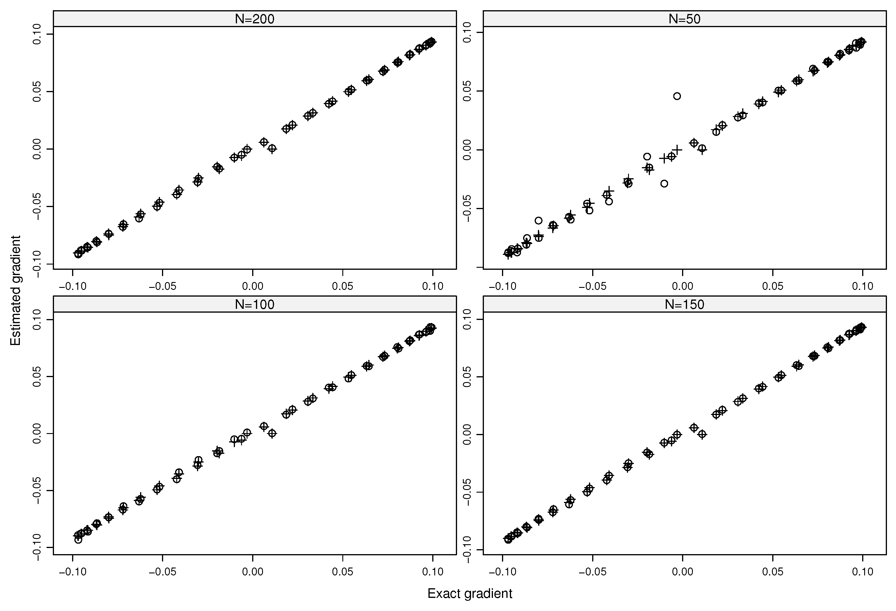
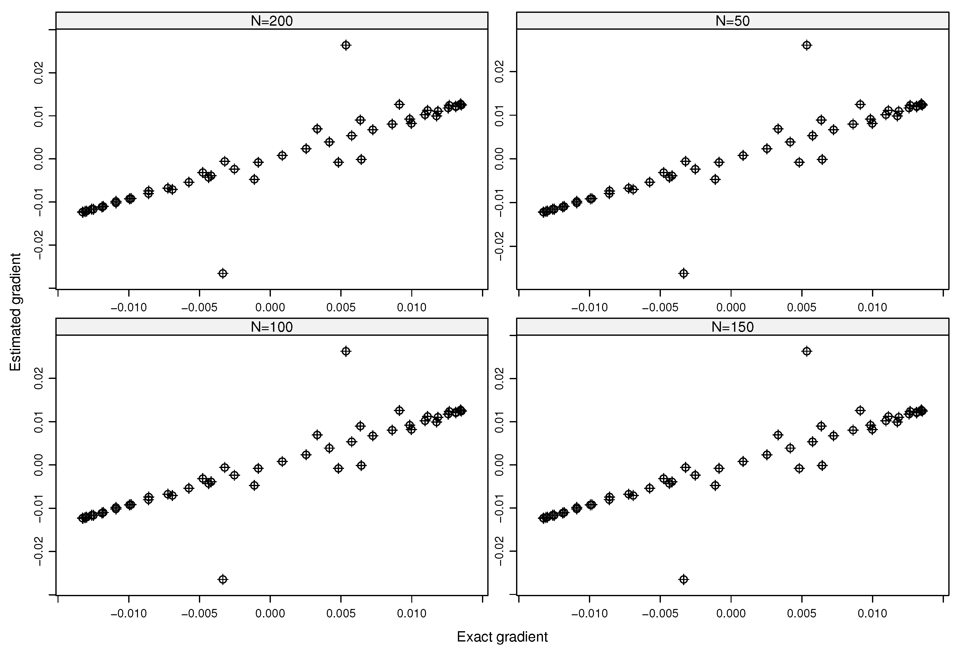
5.3. Comparisons between Exact Gradient and Estimated Gradients

For running the above PDE-based model using the R package deSolve [45], we are given $D=0.0011$ and $s=1.96$. The exact and formal gradient associated with the mean values of the initial conditions is obtained by running the corresponding adjoint model. For estimating the gradient using the proposed estimators, we consider $L=2,3$ and $N=50,100,150,200$. We also use $h=1/\sqrt{N}$ and $V_j\sim \mathcal{N}(0,1),j=1,\dots ,d=50$. The Sobol sequence is used for generating the random values of the $V_j$s, and the Gram–Schmidt algorithm is applied to obtain perfect orthogonal vectors for a given N.

Figure 1 shows the comparisons between the estimated and the exact values of the formal gradient $\nabla f$ (i.e., $\rho (X_{j_1},Z_{j_2})=0$) for $L=1,2$. Likewise, Figure 2 and Figure 3 depict the dependent gradient $grad\left(f\right)={\left({\mathcal{R}}^T\mathcal{R}\right)}^{-1}\nabla f$ and its estimation. The estimates of both gradients are in line with the exact values using only $NL=50$ (respectively, $NL=100$) model evaluations when $L=1$ and $N=50$ (respectively, $L=1$ and $N=100$ or $L=2$ and $N=50$). Increasing the values of L and N gives the same quasiperfect results for both the formal and dependent gradients (see Figure 3).

Figure 1. Exact gradient versus estimated gradients using $L=1$ (∘) and $L=2$ (+) of the QoI by considering the inputs as independent (formal gradients).

Figure 2. Exact gradient versus estimated gradients using $L=1$ (∘) and $L=2$ (+) of the QoI by considering the autocorrelations among the inputs (dependent gradients).

Figure 3. Exact gradient versus estimated gradients using $L=2$ (∘) and $L=3$ (+) of the QoI by considering the autocorrelations anong the inputs (dependent gradients).

6. Conclusions

In this paper, we have proposed new, simple, and generic approximations of the gradients of functions with nonindependent input variables by means of independent, central, and symmetric variables and a set of constraints. It comes out that the biases of our approximations for a wide class of functions, such as 2-smooth functions, do not suffer from the curse of dimensionality by properly choosing the set of independent, central, and symmetric variables. For functions including only independent input variables, a theoretical comparison has shown that the upper bounds of the bias of the formal gradient derived in this paper outperformed the best known results.

For computing the dependent gradient of the function of interest, we have provided estimators of such a gradient by making use of evaluations of that function at $LN$ randomized points. Such estimators reach the optimal (mean squared error) rates of convergence (i.e., $\mathcal{O}\left(N^{-1}{d}^2\right)$) for a wide class of functions. Numerical comparisons using a test case and simulations based on a PDE model with given autocollaborations among the initial conditions have shown the efficiency of our approach, even when $L=1,2$ constraints were used. Our approach is therefore flexible, thanks to L and the fact that the gradient can be computed for every value of the sample size N in general.

While the proposed estimators reach the parametric rate of convergence, note that the second-order moments of such estimators depend on $d^2$. An attempt to reach a dimension-free rate of convergence requires working in $\mathbb{C}$ rather than $\mathbb{R}$ when $L=2$. In the future, it is worth investigating the derivation of the optimal rates of convergence that are dimension-free or (at least) are linear with respect to d by considering $L>3$ constraints. Also, combining such a promising approach with a transformation of the original space might be helpful for reducing the number of model evaluations in higher dimensions.