Abstract
Thin-Plate Spline Generalized Linear Models (TPS-GLMs) are an extension of Semiparametric Generalized Linear Models (SGLMs), because they allow a smoothing spline to be extended to two or more dimensions. This class of models allows modeling a set of data in which it is desired to incorporate the non-linear joint effects of some covariates to explain the variability of a certain variable of interest. In the spatial context, these models are quite useful, since they allow the effects of locations to be included, both in trend and dispersion, using a smooth surface. In this work, we extend the local influence technique for the TPS-GLM model in order to evaluate the sensitivity of the maximum penalized likelihood estimators against small perturbations in the model and data. We fit our model through a joint iterative process based on Fisher Scoring and weighted backfitting algorithms. In addition, we obtained the normal curvature for the case-weight perturbation and response variable additive perturbation schemes, in order to detect influential observations on the model fit. Finally, two data sets from different areas (agronomy and environment) were used to illustrate the methodology proposed here.
Keywords:
exponential family; smoothing spline; penalized likelihood function; weighted back-fitting algorithm; diagnostics measures MSC:
62P12; 62J20; 62G05
1. Introduction
Thin-Plate Spline Generalized Linear Models (TPS-GLMs) represent an extension of semiparametric generalized linear models (SGLMs) by enabling the application of smoothing splines in multiple dimensions. These models have the same characteristics of the generalized linear model (GLM), as described by McCullagh and Nelder [1]. Like GLMs, TPS-GLMs can assume a variety of distribution families for the response variable. They also allow for a non-linear relationship between the response variable’s mean and the linear predictor via a link function, and they account for non constant variance in the data. Furthermore, the TPS-GLM allow modeling non-linear joint interaction effects due to some covariates, as well as the effects of coordinates in spatial data, making them a useful tool to model dynamic pattern in different scientific areas, such as environment, agronomy, ecology, and so on. Some of the main works related to thin-plate spline technique are Duchon [2,3], Bookstein [4], and Chen et al. [5], while in the context of statistical modeling, Wahba [6], Green and Silverman [7], Wood [8], and Moraga et al. [9], can be mentioned, among others.
However, it is well known that diagnostic analysis is a fundamental process in all statistical modeling for any data set. This analysis allows us to validate the assumptions established about the model in question and identify discrepant observations, and eventually influential ones on the fit of the model. One of the main diagnostic techniques used in GLM and SGLM is local influence. In general, the idea of the local influence technique introduced by Cook [10] is to evaluate the sensitivity of the MLEs when small perturbations are introduced in the assumptions of the model or in the data, both in the response variable and in the explanatory variables. This technique has the advantage, regarding the case elimination technique, that it is not necessary to calculate the estimates of the parameters for each case excluded. In our case, we are interested in developing the local influence technique in the TPS-GLM, in order to detect observations that may have a disproportionate influence on the estimators of both the parametric (regression coefficient) and non-parametric (surface) part of the linear predictor. Such influence may be due, for example, to the fact that each experimental unit contributes differently to the model or that our variable of interest is exposed to a certain modification. In the context of GLM and SGLM, there is empirical evidence that the maximum likelihood estimators (MLEs) and maximum penalized likelihood estimators (PMLEs) are sensitive to this type of situation, and therefore we believe that this sensitivity is also present in the estimators of the TPS-GLM, in particular, in the surface estimator.
Various studies have expanded upon the technique of local influence within different parametric models. Thomas and Cook [11] applied Cook’s method of local influence [10] to generalized linear models to assess the impact of minor data perturbations. Ouwens and Beger [12] obtained the normal curvature under a generalized linear model in order to identify influential subjects and/or individual observations. Zhu and Lee [13] developed the local influence technique for incomplete data, and extended such results to generalized linear mixed models (see also Zhu and Lee [14] for further details). Espinheira et al. [15] extended the local influence analysis to beta regression models considering various perturbation scenarios. Rocha and Simas [16] and Ferrari et al. [17] derived the normal curvature considering a beta regression model whose dispersion parameter varies according to the effect of some covariates. Ferreira and Paula [18] developed the local influence approach to partially linear Skew Normal models under different perturbation schemes, and Emami [19] evaluated the sensitivity of Liu penalized least squares estimators using local influence analysis. Most recently, Liu et al. [20] have reported the implementation of influence diagnostics in AR time series models with Skew Normal (SK) distributions.
Within a semiparametric framework, Thomas [21] developed diagnostics for local influence to assess the sensitivity of estimates for the smoothing parameter, which were determined using the cross-validation criterion. Zhu and Lee [14] and Ibacache-Pulgar and Paula [22] introduced measures of local influence to analyze the sensitivity of maximum penalized likelihood estimates in normal and partially linear Student-t models, respectively. Ibacache-Pulgar et al. [23,24] explored local influence curvature within elliptical semiparametric mixed models and symmetric semiparametric additive models. Subsequently, ref. [25] and Ibacache-Pulgar and Reyes [26] further extended local influence measures to normal and elliptical partially varying-coefficient models, respectively. Ibacache-Pulgar et al. [27] developed the local influence method within the context of semiparametric additive beta regression models. Meanwhile, Cavieres et al. [28] calculated the normal curvature to assess the sensitivity of estimators in a thin-plate spline model that incorporates skew normal random errors. Jeldes et al. [29] applied the partially coefficient-varying model with symmetric random errors to air pollution data from the cities of Santiago, Chile, and Lima, Peru. In this context, they carried out an application of the local influence technique to detect influential observations in the model fit. Saavedra-Nievas et al. [30] extended the local influence technique for the spatio-temporal linear model under normal distribution and with separable covariance. Recently, Sánchez et al. [31] obtained the normal curvature for the varying-coefficient quantile regression model under log-symmetric distributions, and presented an interesting application of such results to an environmental pollution data set.
In this work, we extend the local influence approach in Thin-Plate Spline Generalized Linear Model.
The contents are organized as follows: Section 2 introduces the thin-plate spline generalized linear model. Section 3 details the method for obtaining maximum penalized likelihood estimators and discusses some statistical inferential results. In Section 4, we provide a detailed description of the local influence method and derives normal curvatures for various perturbation schemes. In Section 5, the methodology is illustrated using two datasets. The paper concludes with some final observations in Section 6.
2. The Thin-Plate Spline Generalized Linear Model (TPS-GLM)
In this section, we present the TPS-GLM and the penalized function to carry out the process of estimating the parameters.
2.1. Statistical Model
Let be a data set where each response variable follows a distribution from the exponential family with the following density function:
where is the canonical form of the location parameter and depends on the mean . The term represents a known function of the unknown dispersion parameter (or a vector of unknown dispersion parameters). The function c depends on both the dispersion parameter and the responses, while is a known function, such that the mean and variance of are given by: and , with , respectively. The TPS-GLM is defined by Equation (1) and the following systematic component:
where is a vector of covariables, corresponds to the vector of regression coefficients, is unknown smooth arbitrary surface, and is a two-dimensional covariates vector. To write the model given by Equation (1) in a matrix form, first consider the one-to-one transformation of the vector suggested by Green and Silverman [7], stated as
where is a vector with components , is a vector with components , is a matrix whose elements are given by , with for each i, and is a matrix defined as
Thus, the Model (1) can be written in a matrix form as
where the regression matrix is structured as , with , and the vector of regression coefficients as , where () and (); see [9]. Note that this matrix representation of the linear predictor allows us to treat the TPS-GLM as a semiparametric generalized linear model, in which the term represents the parametric component and the nonparametric component. One of the advantages of the TPS-GLM, apart from being able to model both discrete and continuous variables that belong to the exponential family, is its flexibility to model the non-linear joint effect of covariates through the surface f present in the linear predictor . In the context of spatial data, this models allows the effect of coordinates to the incorporated into the modeling process. It is important to note that when the surface f is not present in the linear predictor , the model reduces to the classical generalized linear model. However, if the vector reduces to a scalar, , the model reduces to the semiparametric generalized linear model discussed, for instance, by Green and Silverman [7].
2.2. Penalized Function
Under the TPS-GLM, we have that , with parameters. Then, the log-likelihood function is given by
where
To ensure the identifiability of the parameter vector , we assume that f belongs to the function space where all partial derivatives of total order m reside within the Hilbert space , the space of square-integrable functions on Euclidean d-space. Incorporating a penalty function over f, we have that the penalized log-likelihood function can be expressed as (see, for instance, Green and Silverman [7])
where is a penalty functional measuring the wiggliness of f, and is a constant that depends on the smoothing parameter . In general, a measure of the curvature of f corresponds to its squared norm, , defined as
For simplicity, in this work, we will consider the case in which and . Consequently, the penalty function is expressed in the form
and measures the rapid variation in f and the departure from local linearity. In this case, the estimation of f leads to a natural thin-plate spline. According to Green and Silverman [7], we may express the penalty functional as . Then, if we consider , the penalized log-likelihood function (3) can be expressed as
The first term in the right-hand side of Equation (4) measures the goodness-of-fit, while the second terms penalizes the roughness of f with a fixed parameter . Selecting appropriate parameters is crucial in the estimation process, as they determine the balance between the goodness-of-fit and the smoothness (or regularity) of the estimated function. It is important to emphasize that selecting appropriate parameters is crucial in the estimation process because they control the trade-off between goodness-of-fit and the smoothness (or regularity) of the estimated function. In this work, the smoothing parameter is selected through the Akaike Criterion (AIC) based on the penalized log-likelihood function given in Equation (3). More details of the method are given in Section 3.7.
3. Estimation and Inference
In this section, we discuss the problem of estimating the parameters under the TPS-GLM. Specifically, we derive a weighted iterative process based on the backfitting algorithm and estimate the variance–covariance matrix of our estimator from the penalized Fisher information matrix (see Green [32] and Green and Silverman [7]). A brief discussion of the smoothing parameter selection is also presented.
3.1. Penalized Score Function
First, we are going to assume that the function is regular in the sense that it admits first and second partial derivatives with respect to the elements of the parameter vector . To obtain the score function for , we must calculate for i ∈ and j ∈ . After performing some partial derivative operations, we have that the score function for can be written in matrix as follows:
where is an () matrix whose ith row is , is a () matrix, with the variance function, a function of , and are () vectors.
Conversely, to derive the score function for , we need to compute for i ∈ and ℓ ∈ . Again, after some algebraic operations, the score function for can be written in matrix as follows:
where the matrix is defined in Section 2.1. Finally, the score function for is given by
with , for i ∈ . Thus, the vector of penalized score functions of can be expressed compactly as
Note that if the model under consideration only considers the parametric component in the linear predictor, that is, the nonparametric component is omitted, the expressions of the remaining score functions are reduced to those obtained under the classical generalized linear model.
3.2. Penalized Hessian Matrix
To obtain the penalized Hessian matrix, we must compute the second-derivate of with respect to each element of , that is, , for ∈ . After some algebraic operations, we have that the diagonal elements (block matrices) of the Hessian matrix are given by
where and , for . The elements outside the main diagonal of the Hessian matrix take the form
where denotes the th element of the matrix and denotes the th element of the matrix , for i ∈ , j ∈ and ℓ ∈ . Thus, the penalized Hessian matrix can be represented as
It is noteworthy that this matrix simplifies to the Hessian matrix used in generalized linear models when the nonparametric component is absent. The primary application of this matrix lies in the normal curvature, which is essential for developing the local influence technique. This will be discussed in the following section.
3.3. Penalized Expected Information Matrix
By taking the expectation of the matrix , we derive the penalized expected information matrix, which is of dimension , as follows:
This matrix assumes the following diagonal structure in blocks:
where
and
with for i ∈ .
3.4. Derivation of the Iterative Process
The value of that maximizes , called maximum penalized likelihood estimate (MPLE) and denoted by , is carried out by solving the corresponding estimation equations. Let , where and . In addition, consider the partition of the score function vector , where and . In order to estimate based on penalized likelihood function given by Equation (4), we have to solve the equations
These estimating equations are nonlinear, and necessitate an iterative approach for their solution. An alternative frequently proposed in the context of generalized linear models is the Fisher scoring algorithm (Nelder and Wedderburn, [33]), considering the fact that in some situations the matrix can be non-positive definite. Then, the algorithm for estimating , with fixed, is given by
which is equivalent to solving the matrix equation
where , with defined as
Consequently, the weighted back-fitting (Gauss–Seidel) iterations for simultaneously updating and are given by
It is crucial to note that the system of Equations (5) is consistent, and the back-fitting algorithm converges to a solution for any initial values, provided that the weight matrix is symmetric and positive definite. Additionally, if the parametric component is absent in the linear predictor, the estimator of is given by:
The MPLE of the dispersion parameter, , can be determined through the following iterative procedure:
3.5. Estimation of Surface
To obtain the MPLE of f, we must consider its one-to-one representation given in Equation (2) and MPLE obtained from the iterative process described above. Indeed, we have that can be obtained as
where and are the MPLE of and , respectively. Note that vector corresponds to the first three elements of vector . Consequently, is a natural thin-plate spline. Details of the conditions that guarantee this result are given, for example, in Green and Silverman [7] and Wood [34].
3.6. Approximate Standard Errors
In this study, we propose approximating the variance–covariance matrix of by using the inverse of the penalized Fisher information matrix. Specifically, we have that
If we are interested in drawing inferences for , the approximate variance–covariance matrix can be estimated by using the corresponding block-diagonal matrix obtained from , similarly for and .
3.7. On Degrees of Freedom and Smoothing Parameter
For the TPS-GLM, the degree of freedom () associated with the smooth surface is given by (see, for instance Green and Silverman [7])
which approximately represents the number of effective parameters used in the modeling process to estimate the smooth surface f.
Regarding the selection of the smoothing parameter, we propose to use the Akaike Information Criterion (AIC) (see, for instance, [24,35]), defined as
where denote the penalized likelihood function evaluated at MPLE of , and p denote the number of parameters in . As usual, the idea is to select the value of that minimizes .
4. Local Influence
In this section, we extend the local influence technique to evaluate the sensitivity of the MPLE under the TPS-GLM. Specifically, we present some theoretical aspects of the method and, subsequently, we derive the normal curvature for three perturbation schemes.
4.1. Local Influence Analysis
Consider , an vector of perturbations restricted to some open subset . Let denote the logarithm of the perturbed penalized likelihood function. Assume there exists a vector of non-perturbation , such that . To evaluate the influence of small perturbations on the MPL estimate , we can consider the penalized likelihood displacement given by:
where is the MPL estimate under . The measure LD() is useful for assessing the distance between and . Cook [10] suggested examining the local behavior of LD() around . The procedure involves selecting a unit direction , with , and then plotting LD() against a, where . This plot, called the lifted line, can be characterized by considering the normal curvature around . The suggestion is to assume the direction corresponding to the largest curvature . The index plot of can identify those cases that, under small perturbations, have a significant potential influence on LD(). According to Cook [10], the normal curvature in the unit direction is expressed as
with
Note that represents the penalized observed information matrix evaluated at (see Section 3.2), and is the penalized perturbation matrix evaluated at and . It is essential to highlight that denotes the local influence on the estimate after perturbing the model or data. Escobar and Meeker [36] suggested examining the normal curvature in the direction , where is an vector with a one at the ith position and zeros elsewhere. Consequently, the normal curvature, referred to as the total local influence of the ith case, takes the form for , where is the ith principal diagonal element of the matrix .
4.2. Derivation of the Normal Curvature
Typically, the perturbation schemes used in the analysis of local influence are determined by the structure of the model under consideration, as discussed by Billor and Loynes [37]. These schemes can generally be divided into two main categories: perturbations to the model (to examine changes in assumptions) or perturbations to the data. For instance, we might consider perturbing the response variable or the explanatory variables. The motivation for employing these perturbation schemes often includes addressing issues such as the presence of outliers or the occurrence of measurement errors in the data. Subsequently, we will present the formulas for the matrix for various perturbation schemes.
Consider the weights assigned to the observations in the penalized log-likelihood function, given by:
where , is the vector of weights, with . In this case, the vector of no perturbation is given by . Differentiating with respect to the elements of and , we have that the matrix takes the form
where the matrix and , with , , denotes the inverse function of , , and a vector with 1 at the ith position and zero elsewhere.
To perturb the response variable values, we consider for , where is the vector of perturbations. The vector of no perturbation is . The perturbed penalized log-likelihood function is constructed from Equation (3) with replaced by , as follows:
where is defined in Equation (2) with replacing . By differentiating with respect to the elements of and , and after some algebraic manipulation, we obtain:
where the matrix and , with and , with denoting a vector with 1 at the ith position and zero elsewhere.
5. Applications
In this section, we show the applicability of the TPS-GLM and the local influence method with two real data applications. The model estimation and diagnostics have been implemented using MatLab 9.13.0 (R2022b) software [38] (the developed code is available on request by the authors).
5.1. Wypych Data
The first dataset we use to illustrate the applicability of the TPS-GLM consists of 83 sample points within a 46.6-hectare agricultural area in Wypych, located at latitude 24°50′24″ S and longitude 53°36′36″ W, with an average altitude ranging from 589 to 660 m. The data were collected during the 2006/2007 agricultural year in the western region of Paraná State, Brazil (see [39], Appendix 4). The soil is classified as Dystroferric Red Latosol with a clayey texture. The region’s climate is mesothermal, super-humid temperate, classified as Cfa according to (Köeppen), with a mean annual temperature of 21 °C. The 83 georeferenced points were determined by a regular grid of m using a global positioning system (GPS). The collected variables were as follows:
- Soya: average of soybean yield (t/ha).
- Height: average height (cm)of plants at the end of the production process.
- Pods: average number of pods.
- Lat: latitude (UTM).
- Long: longitude (UTM).
The original objective was to investigate the spatial variability of soybean yield (Soya) in the studied area based on the covariates: average plant height, average number of pods per plant, latitude, and longitude. Figure 1 shows the scatterplots between the response variable Soya and the explanatory variables Height and Pods. In addition, the plot of the response variable against the coordinates is shown. Clearly, from Figure 1a,b, it can be seen that the explanatory variables Height (X2) and Pods (X3) are linearly related to the response variable Soya (Z). The spatial effect given by the coordinates (X,Y) will be incorporated into the model through a smooth surface.
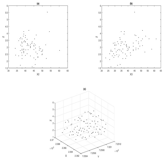
Figure 1.
Scatter plots: Soya versus Height (a), Soya versus Pods (b), and Soya versus coordinates in UTM (c).
5.1.1. Fitting the TPS-GLM
Based on the above analysis, we propose the TPS-GLM, introduced in Section 2, to model the trends present in the Wypych data. Specifically, we are going to assume that the response variable Soya belongs to the Gaussian family, and that the link function is the identity. Therefore, the model is expressed as follows:
where correspond to the regression coefficients associated with the parametric component of the model, and is a smooth surface. Table 1 lists the MPLE of . The respective asymptotic standard errors are presented in parentheses.

Table 1.
MPLEs with their standard errors (within parenthesis), AIC and R2(Adj).
The value of the smoothing parameter was selected in such a way that the AIC criterion was minimized. The adjusted determinant coefficients (R2(Adj)) are evaluated for assessing the goodness-of-fit of the two models. It is important to note that our model have a lower AIC and an higher R2(Adj), compared to the multiple regression model that does not consider the spatial effect. Figure 2a shows the QQ-plot for the standardized residuals, whose adjustment to the Gaussian TPS-GLM seems to be reasonable. However, the presence of some atypical observations is observed in one of the tails of the distribution. Figure 2b displays the scatter plot between the observed values, Soya, and their estimated values, . Considering the trend of the points, we conclude that the estimates are good, since they generate consistent adjusted values of the response variable.
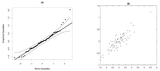
Figure 2.
QQ-plots of the standardized residuals for the TPS-GLM with its confidence interval (dashed lines) (a) and scatterplot between Soya and (b), under model fitted to Wypych data.
5.1.2. Diagnostic Analysis
To identify potentially influential observations on the MPLE under the fitted Gaussian TPS-GLM for the Wypych data, we present several index plots of for . Figure 3 shows the index plot for the case-weight perturbation scheme under the fitted model. Figure 3a reveal that the observations , , and are more influential on , whereas the observations , , and are more influential on ; see Figure 3b. When we perturb the response variable additively, we have that the observations , , and are more influential on ; see Figure 4a. Regarding , observations , and appear as slightly influential as seem in Figure 4b.
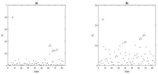
Figure 3.
Index plots of for assessing local influence on (a) and (b), considering case-weight perturbation.
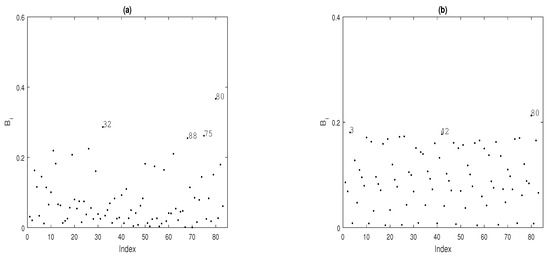
Figure 4.
Index plots of for assessing local influence on (a) and (b), considering response variable additive perturbation.
We conclude that the maximum penalized likelihood estimates (MPLE) of the regression coefficients and the smooth surface exhibit sensitivity to modifications made to the data or the model. This analysis has shown that observations identified as influential for the parametric component do not necessarily exert influence on the non-parametric component, and vice versa. For instance, under the case-weight perturbation scheme, observations and were detected as influential for the parametric component, but not for the nonparametric component.
5.1.3. Confirmatory Analysis
Table 2 displays the relative changes experienced by each element in the vector of regression coefficients. In this analysis, we only consider the three most influential observations under the case-weight perturbation scheme. As can be seen in this table, observations , and generate significant changes in the estimates. Still, no relevant inferential changes were noted. However, the AIC and &R2(Adj) present some differences once the above observations are dropped.

Table 2.
Relative changes (RCs) (in %) in the MPL estimates of in cases-weight perturbation under the TPS-GLM. The last two columns indicate the AIC and R2(Adj) of the model with dropped observations.
On the other hand, Table 3 shows the relative changes in the vector of regression coefficients under the additive perturbation scheme of the response variable. Here, we consider the four most influential observations. As can be seen in the table, observations , , and generate important relative changes in the estimates of the parametric component of the model. However, no significant inferential changes were observed. About the AIC and &R2(Adj), there are not evident differences.

Table 3.
Relative changes (RCs) (in %) in the MPL estimates of in response variable perturbation under the TPS-GLM. The last two columns indicate the AIC and R2(Adj) of the model with dropped observations.
5.2. Ozone Concentration Data
For our analysis, we utilize data from a study examining the relationship between atmospheric ozone concentration (O3) and various meteorological variables in the Los Angeles Basin for a sample of 330 days in 1976. The data were initially presented by Breiman and Friedman [40], and are available for download from various public repositories. Although the dataset includes several variables, in this application, we will consider only three explanatory variables, which are detailed in the following.
- O3: daily maximum one-hour average ozone concentration in Upland, CA, measured in parts per million (ppm).
- Temp: Sandburg Air Base temperature, in Celsius.
- Vis: visibility, in miles.
- Day: calendar day.
Figure 5 contains the dispersion graphs between the outcome variable (log(O3)) and each one of the explanatory variables Temp, Vis and Day.
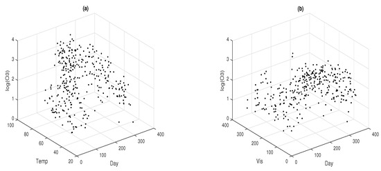
Figure 5.
3D plots between the response variable and the explanatory variables: logarithm of ozone data versus temperature and day variables (a), and logarithm of ozone data versus visibility and day variables (b).
Figure 5a shows a curved surface in the relationship between the variable log(O3) and the joint effect of the explanatory variables Temp and Day, whereas the relationship between log(O3) and the joint effect of the explanatory variable Vis and Day shows less curve; see Figure 5b. This graphical analysis recommends the inclusion in the model of a nonparametric component, specifically a surface, that can explain the relationship between log(O3) and the combined effect of the explanatory variables Temp and Day. For simplicity, in this work, we will include the effect of the explanatory variable Vis in a linear form. To begin our analysis, we are going to consider the fit of a GLM assuming that the variable of interest O3 is Poisson distributed with mean and logarithmic link function. Different structures of the linear predictor for the explanatory variables Vis, Temp, and Day will be considered (see Table 4).

Table 4.
Four structures of the linear predictor for the explanatory variables Vis, Temp, and Day, assuming that the response variable log(O3) follows a distribution.
For Model I, we consider only the individual effects of the explanatory variables Vis, Temp and Day. Note that all these effects were incorporated in a linear form in the systematic component of the model. For Model II, we consider the inclusion of a nonparametric term to model the nonlinear effects of the explanatory variable Day; see Ibacache et al. [41]. Model III considers a systematic component that contains the individual effects of the explanatory variables Vis, Temp and Day, in addition to the incorporation of the interaction effect between the explanatory variables Temp and Day. Here, the interaction effect is introduced linearly in the model. Model IV corresponds to a TPS-GLM where the joint effect of the Temp and Day explanatory variables is included nonlinearly by using smooth surface. Table 5 contains the ML and MPL estimates associated with the parametric component for the four fitted models.

Table 5.
AIC, R2(Adj), ML and MPL estimates for all four fitted models to the Ozone data.
It is important to note that both the individual and interaction effects are statistically significant, as the corresponding p-values (not shown here) are less than 0.05. Additionally, the estimates of are similar across the four models, whereas the estimates of vary considerably, particularly in Model IV. Concerning the associated standard errors, all the estimators exhibit small values. The last two rows of Table 5 display the Akaike Information Criterion (AIC) and values, respectively. It is evident that the TPS-GLM, with AIC, provides the best fit to the Ozone data, followed by Model II with an AIC of 1806.837. This is corroborated by the QQ-plots in Figure 6, specifically Figure 6b,d. Furthermore, the value associated with our model is higher than those of Models I, II, and III. The smoothing parameter was chosen such that the effective degrees of freedom were approximately 7. Figure 7 illustrates the 3D plot of the adjusted log(O3) against the explanatory variables Temp and Day, showing an adequate fit of the TPS-GLM.
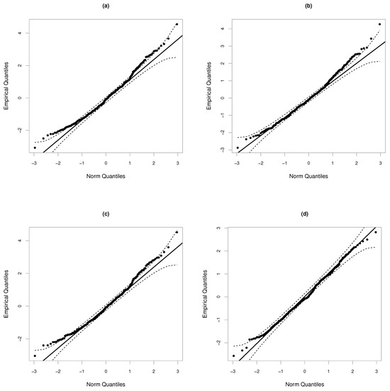
Figure 6.
QQ-plot of the standardized residuals for the models described in Table 5: Model I (a), Model II (b), Model III (c) and Model IV (d).
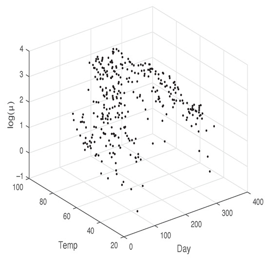
Figure 7.
3D plot between and explanatory variables Temp and Day.
5.2.1. Diagnostic Analysis
To identify potentially influential observations on the MPL estimators under the fitted TPS-GLM for the Ozone data, we present some index plots of , for . Figure 8 shows the index plot of for the case-weight perturbation scheme under the fitted model. In Figure 8a,b, note that observations , , , and are more influential on and , respectively. By perturbing the response variable additively, it becomes clear that observations , , , , and are more influential on and ; see Figure 9a and Figure 9b, respectively.
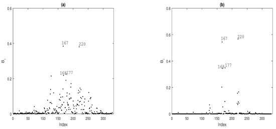
Figure 8.
Index plots of for assessing local influence on (a) and (b), considering case-weight perturbation under model fitted to Ozone data.
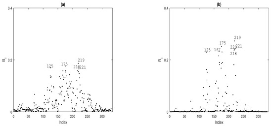
Figure 9.
Index plots of for assessing local influence on (a) and (b), considering response variable additive perturbation.
From the local influence analysis, we conclude that the MPLE of the regression coefficients and the smooth surface are sensitive to perturbations in the data or the model. Furthermore, this analysis revealed that observations identified as influential for the parametric component are also influential for the nonparametric component, and vice versa. For example, under the case-weight perturbation scheme, observations , , , and were found to be influential for both the parametric and nonparametric components.
5.2.2. Confirmatory Analysis
To investigate the impact on model inference when influential potentially observations detected in the diagnostic analysis are removed, we present the relative changes (RCs) in the MPL estimate of for after removing the influential observations from the dataset (%). The RC is defined as , where denotes the MPL estimate of , with , after the corresponding observation(s) are removed according to set I. Table 6 presents the RCs in the regression coefficient estimates after removing the observations identified as potentially influential for the parametric component of the model.

Table 6.
Relative changes (RCs) (in %) in the MPL estimates of under the TPS-GLM. The last two columns indicate the AIC and R2(Adj) of the model with dropped observations.
6. Concluding Remarks and Future Research
In this work, we study some aspects of the Thin-Plate Spline Generalized Linear Models. Specifically, we derive an iterative process to estimate the parameters and the Fisher information matrix to approximate, through its inverse, the variance–covariance matrix of the estimators. In addition, we extended the local influence method, obtaining closed expressions for the Hessian and perturbation matrices under cases-weight perturbation and additive perturbation of the response variable. We performed a statistical data analysis with two real data sets of the agronomic and environmental area. The study showed the advantage of incorporating a smooth surface to model the joint effect of a pair of explanatory variables or the spatial effect determined by the coordinates. In both applications, it was observed that the adjusted values of the response variable were consistent. In addition, it was observed that our model presented a better fit to model the soybean yield and ozone concentration data, compared to some classic parametric and semiparametric models, respectively. In our analysis, it was found that those observations detected as potentially influential generated important changes in the estimates, but not significant inferential changes. In addition, our study confirms the need to develop the local influence method to evaluate the sensitivity of maximum penalized likelihood estimators and thus determine those observations that can exert an excessive influence on both the parametric and non-parametric components, or on both.
As future work, we propose to incorporate a correlation component in the model and extend the local influence technique to other perturbation schemes, mainly on the non-parametric component of the model.
Author Contributions
Conceptualization, G.I.-P., P.P., M.A.U.-O. and O.N.; methodology, G.I.-P. and O.N.; software, G.I.-P. and P.P.; validation, G.I.-P. and P.P.; formal analysis, P.P.; investigation, G.I.-P., P.P., O.N. and M.A.U.-O.; data curation, P.P. and M.A.U.-O.; writing—original draft preparation, G.I.-P. and P.P.; writing—review and editing, O.N. and M.A.U.-O.; supervision, G.I.-P. and O.N.; project administration, O.N.; funding acquisition, O.N. All authors have read and agreed to the published version of the manuscript.
Funding
This research was funded by ANID-Fondecyt grant number 1201478.
Institutional Review Board Statement
Not applicable.
Informed Consent Statement
Not applicable.
Data Availability Statement
Data cannot be shared openly but are available on request from authors.
Acknowledgments
The third author acknowledges the support of ANID-Fondecyt 1201478.
Conflicts of Interest
The authors declare no conflicts of interest.
References
- McCullagh, P.; Nelder, J.A. Generalized Linear Models, 2nd ed.; Chapman and Hall: London, UK, 1989. [Google Scholar]
- Duchon, J. Interpolation des fonctions de deux variables suivant le principe de la flexion des plaques minces. RAIRO Anal. Numér. 1976, 10, 5–12. [Google Scholar] [CrossRef]
- Duchon, J. Splines minimizing rotation-invariant semi-norms in Sobolev spaces. Lect. Notes Math. 1977, 57, 85–100. [Google Scholar]
- Bookstein, F.L. Principal warps: Thin-plate splines and decomposition of deformations. IEEE Trans. Pattern Anal. Mach. Intell. 1989, 11, 567–585. [Google Scholar] [CrossRef]
- Chen, C.; Li, Y.; Yan, C.; Dai, H.; Liu, G. A Thin Plate Spline-Based Feature-Preserving Method for Reducing Elevation Points Derived from LiDAR. Remote Sens. 2015, 7, 11344–11371. [Google Scholar] [CrossRef]
- Wahba, G. Spline Models for Observational Data; SIAM: Philadelphia, PA, USA, 1990. [Google Scholar]
- Green, P.J.; Silverman, B.W. Nonparametric Regression and Generalized Linear Models; Chapman and Hall: Boca Raton, FL, USA, 1994. [Google Scholar]
- Wood, S.N. Thin plate regression splines. J. R. Stat. Soc. Ser. B (Methodol.) 2003, 65, 95–114. [Google Scholar] [CrossRef]
- Moraga, M.S.; Ibacache-Pulgar, G.; Nicolis, O. On an elliptical thin-plate spline partially varying-coefficient model. Chil. J. Stat. 2021, 12, 205–228. [Google Scholar]
- Cook, R.D. Assessment of Local Influence. J. R. Stat. Soc. Ser. B (Methodol.) 1986, 48, 133–169. [Google Scholar] [CrossRef]
- Thomas, W.; Cook, R.D. Assessing influence on regression coefficients in generalized linear models. Biometrika 1989, 76, 741–749. [Google Scholar] [CrossRef]
- Ouwens, M.N.M.; Tan, F.E.S.; Berger, M.P.F. Local influence to detect influential data structures for generalized linear mixed models. Biometrics 2001, 57, 1166–1172. [Google Scholar] [CrossRef]
- Zhu, H.; Lee, S. Local influence for incomplete-data models. J. R. Stat. Soc. Ser. B 2001, 63, 111–126. [Google Scholar] [CrossRef]
- Zhu, H.; Lee, S. Local influence for generalized linear mixed models. Can. J. Stat. 2003, 31, 293–309. [Google Scholar] [CrossRef]
- Espinheira, P.L.; Ferrari, P.L.; Cribari-Neto, F. Influence diagnostics in beta regression. Comput. Stat. Data Anal. 2008, 52, 4417–4431. [Google Scholar] [CrossRef]
- Rocha, A.; Simas, A. Influence diagnostics in a general class of beta regression models. TEST 2001, 20, 95–119. [Google Scholar] [CrossRef]
- Ferrari, S.; Spinheira, P.; Cribari-Neto, F. Diagnostic tools in beta regression with varying dispersion. Stat. Neerl. 2011, 65, 337–351. [Google Scholar] [CrossRef]
- Ferreira, C.S.; Paula, G.A. Estimation and diagnostic for skew-normal partially linear models. J. Appl. Stat. 2017, 44, 3033–3053. [Google Scholar] [CrossRef]
- Emami, H. Local influence for Liu estimators in semiparametric linear models. Stat. Pap. 2018, 59, 529–544. [Google Scholar] [CrossRef]
- Liu, Y.; Mao, G.; Leiva, V.; Liu, S.; Tapia, A. Diagnostic Analytics for an Autoregressive Model under the Skew-Normal Distribution. Mathematics 2020, 8, 693. [Google Scholar] [CrossRef]
- Thomas, W. Influence diagnostics for the cross-validated smoothing parameter in spline smoothing. J. Am. Stat. Assoc. 1991, 9, 693–698. [Google Scholar] [CrossRef]
- Ibacache, G.; Paula, G.A. Local Influence for student-t partially linear models. Comput. Stat. Data Anal. 2011, 55, 1462–1478. [Google Scholar] [CrossRef]
- Ibacache-Pulgar, G.; Paula, G.A.; Galea, M. Influence diagnostics for elliptical semiparametric mixed models. Stat. Model. 2012, 12, 165–193. [Google Scholar] [CrossRef]
- Ibacache, G.; Paula, G.A.; Cysneiros, F. Semiparametric additive models under symmetric distributions. Test 2013, 22, 103–121. [Google Scholar] [CrossRef]
- Zhang, J.; Zhang, X.; Ma, H.; Zhiya, C. Local influence analysis of varying coefficient linear model. J. Interdiscip. Math. 2015, 3, 293–306. [Google Scholar] [CrossRef]
- Ibacache-Pulgar, G.; Reyes, S. Local influence for elliptical partially varying coefficient model. Stat. Model. 2018, 18, 149–174. [Google Scholar] [CrossRef]
- Ibacache-Pulgar, G.; Figueroa-Zuñiga, J.; Marchant, C. Semiparametric additive beta regression models: Inference and local influence diagnostics. REVSTAT-Stat. J. 2019, 19, 255–274. [Google Scholar]
- Cavieres, J.; Ibacache-Pulgar, G.; Contreras-Reyes, J. Thin plate spline model under skew-normal random errors: Estimation and diagnostic analysis for spatial data. J. Stat. Comput. Simul. 2023, 93, 25–45. [Google Scholar] [CrossRef]
- Jeldes, N.; Ibacache-Pulgar, G.; Marchant, C.; López-Gonzales, J.L. Modeling Air Pollution Using Partially Varying Coefficient Models with Heavy Tails. Mathematics 2022, 10, 3677. [Google Scholar] [CrossRef]
- Saavedra-Nievas, J.C.; Nicolis, O.; Galea, M.; Ibacache-Pulgar, G. Influence diagnostics in Gaussian spatial—Temporal linear models with separable covariance. Environ. Ecol. Stat. 2023, 30, 131–155. [Google Scholar] [CrossRef]
- Sánchez, L.; Ibacache-Pulgar, G.; Marchant, C.; Riquelme, M. Modeling Environmental Pollution Using Varying-Coefficients Quantile Regression Models under Log-Symmetric Distributions. Axioms 2023, 12, 976. [Google Scholar] [CrossRef]
- Green, P.J. Penalized Likelihood for General Semi-Parametric Regression Models. Int. Stat. Rev. 1987, 55, 245–259. [Google Scholar] [CrossRef]
- Nelder, J.A.; Wedderburn, R.W.M. Generalized Linear Models. J. R. Stat. Soc. Ser. A (Gen.) 1972, 135, 370–384. [Google Scholar] [CrossRef]
- Wood, S.N. Generalized Additive Models: An Introduction with R, 2nd ed.; Chapman and Hall/CRC: Boca Raton, FL, USA, 2017. [Google Scholar]
- Akaike, H. Information theory as an extension of the maximum likelihood principle. In Proceedings of the Second International Symposium on Information Theory; Petrov, B.N., Csaki, F., Eds.; Academiai Kiado: Budapest, Hungary, 1973. [Google Scholar]
- Escobar, L.A.; Meeker, W.Q. Assessing Influence in Regression Analysis with Censored Data. Biometrics 1992, 48, 507–528. [Google Scholar] [CrossRef] [PubMed]
- Billor, N.; Loynes, R.M. Local influence: A new approach. Comm. Statist. Theory Meth. 1993, 22, 1595–1611. [Google Scholar] [CrossRef]
- MathWorks Inc. MATLAB Version: 9.13.0 (R2022b); The MathWorks Inc.: Natick, MA, USA, 2022; Available online: https://www.mathworks.com (accessed on 10 October 2022).
- Uribe-Opazo, M.A.; Borssoi, J.A.; Galea, M. Influence diagnostics in Gaussian spatial linear models. J. Appl. Stat. 2012, 3, 615–630. [Google Scholar] [CrossRef]
- Breiman, L.; Friedman, J.H. Estimating optimal transformations for multiple regression and correlation. J. Am. Stat. Assoc. 1985, 80, 580–598. [Google Scholar] [CrossRef]
- Ibacache-Pulgar, G.; Lira, V.; Villegas, C. Assessing Influence on Partially Varying-coefficient Generalized Linear Model. REVSTAT-Stat. J. 2022. Available online: https://revstat.ine.pt/index.php/REVSTAT/article/view/507 (accessed on 10 October 2022).
Disclaimer/Publisher’s Note: The statements, opinions and data contained in all publications are solely those of the individual author(s) and contributor(s) and not of MDPI and/or the editor(s). MDPI and/or the editor(s) disclaim responsibility for any injury to people or property resulting from any ideas, methods, instructions or products referred to in the content. |
© 2024 by the authors. Licensee MDPI, Basel, Switzerland. This article is an open access article distributed under the terms and conditions of the Creative Commons Attribution (CC BY) license (https://creativecommons.org/licenses/by/4.0/).