Conditioning Theory for $\mathcal{ML}$-Weighted Pseudoinverse and $\mathcal{ML}$-Weighted Least Squares Problem

Abstract

The conditioning theory of the $\mathcal{ML}$-weighted least squares and $\mathcal{ML}$-weighted pseudoinverse problems is explored in this article. We begin by introducing three types of condition numbers for the $\mathcal{ML}$-weighted pseudoinverse problem: normwise, mixed, and componentwise, along with their explicit expressions. Utilizing the derivative of the $\mathcal{ML}$-weighted pseudoinverse problem, we then provide explicit condition number expressions for the solution of the $\mathcal{ML}$-weighted least squares problem. To ensure reliable estimation of these condition numbers, we employ the small-sample statistical condition estimation method for all three algorithms. The article concludes with numerical examples that highlight the results obtained.

1. Introduction

The study of generalized inverses of matrices has been a very important research field since the middle of last century and remains one of the most active research branches in the world [1,2,3]. Generalized inverses, including the weighted pseudoinverse, have numerous applications in various fields, such as control, networks, statistics, and econometrics [4,5,6,7]. The $\mathcal{ML}$-weighted pseudoinverse of $m\times n$ matrix $\mathcal{K}$ with the entries of two weight matrices $\mathcal{M}$ and $\mathcal{L}$ (with order $s\times m$ and $l\times n$, respectively) is defined as

$$\begin{array}{c}\hfill {\mathcal{K}}_{\mathcal{M}\mathcal{L}}^{†}=\left(I_n-{\left(\mathcal{L}\mathcal{P}\right)}^{†}\mathcal{L}\right){\left(\mathcal{MK}\right)}^{†}\mathcal{M},\end{array}$$

(1)

where ${\left(\mathcal{MK}\right)}^{†}$ denotes the Moore-Penrose inverse of $\mathcal{MK}$ and $\mathcal{P}=I_n-{\left(\mathcal{M}\mathcal{K}\right)}^{†}\mathcal{M}\mathcal{K}$. The $\mathcal{ML}$-weighted pseudoinverse [3] originated from the $\mathcal{ML}$-weighted least squares problem ($\mathcal{ML}$-WLS), which is stated as follows:

$$\begin{array}{c}\hfill \underset{\begin{array}{c}x\in S\end{array}}{min}{\parallel x\parallel }_{\mathcal{L}}\mathrm{with}S=\left\{{x:\parallel \mathcal{K}x-h\parallel }_{\mathcal{M}}\mathrm{is}\mathrm{minimum}\right\},\end{array}$$

(2)

where ${\parallel ·\parallel }_{\mathcal{L}}$ and ${\parallel ·\parallel }_{\mathcal{M}}$ are the ellipsoidal seminorms

$${\parallel x\parallel }_{\mathcal{L}}^2=x^H{\mathcal{L}}^H\mathcal{L}x,{\parallel h\parallel }_{\mathcal{M}}^2=h^H{\mathcal{M}}^H\mathcal{M}h,$$

with $h\in {\mathbb{R}}^m$. The $\mathcal{ML}$-WLS exists and has a unique solution:

$$\begin{array}{c}\hfill x={\mathcal{K}}_{\mathcal{M}\mathcal{L}}^{+}h+\mathcal{P}\left(I_n-{\left(\mathcal{L}\mathcal{P}\right)}^{+}\mathcal{L}\mathcal{P}\right)z\mathrm{for}\mathrm{some}\mathrm{vector}z,\end{array}$$

(3)

if and only if $rank\left(B\right)=n$, with $B=$$\left(\begin{array}{c}\mathcal{M}\mathcal{K}\\ \mathcal{L}\end{array}\right)$. In this case it can be shown [3] that

$$\mathcal{P}\left(I_n-{\left(\mathcal{L}\mathcal{P}\right)}^{+}\mathcal{L}\mathcal{P}\right)=0.$$

The $\mathcal{ML}$-weighted pseudoinverse ${\mathcal{K}}_{\mathcal{ML}}^{†}$ [8] is helpful in solving $\mathcal{ML}$-WLS problems [2,9], which is a generalization of the equality constraint least squares problem and has been widely explored in the literature (see, e.g., [9,10,11,12]). Eldén [9] studied perturbation theory for this problem, whereas Cox et al. [12] retrieved the upper perturbation bound and provided the normwise condition number. Li and Wang [13] presented structured and unstructured partial normwise condition numbers, whereas Diao [14] provided partial mixed and componentwise condition numbers for this problem. Until today, the condition numbers for the $\mathcal{ML}$-WLS problem were not yet explored. Motivated by this and considering their significance in ELS research, we present explicit representations of the normwise, mixed, and componentwise condition numbers for the $\mathcal{ML}$-WLS problem, as well as statistical estimation.

A large number of articles and monographs have appeared during the last two decades in the literature dealing with the $\mathcal{ML}$-weighted pseudoinverse ${\mathcal{K}}_{\mathcal{ML}}^{†}$ [1,3,8]. The $\mathcal{ML}$-weighted pseudoinverse ${\mathcal{K}}_{\mathcal{ML}}^{†}$ converts to the K-weighted pseudoinverse ${\mathcal{K}}_{\mathcal{L}}^{†}$ [3] when $\mathcal{M}=I$, the generalized inverse ${\mathcal{C}}_{\mathcal{L}}^{‡}$ [15] when $\mathcal{L}$ has a full row rank and $\mathcal{M}=I$, and the Moore-Penrose inverse ${\mathcal{K}}^{†}$ [16] when both $\mathcal{M}=I$, and $\mathcal{L}=I$. Wei and Zhang [8] discussed the structure and uniqueness of the $\mathcal{ML}$-weighted pseudoinverse ${\mathcal{K}}_{\mathcal{ML}}^{†}$. Elden [3] devised the algorithm for ${\mathcal{K}}_{\mathcal{ML}}^{†}$. Wei [17] considered the ${\mathcal{K}}_{\mathcal{L}}^{†}$ expression using GSVD. Gulliksson et al. [18] proposed a perturbation equation for ${\mathcal{K}}_{\mathcal{L}}^{†}$. Galba et al. [4] proposed iterative methods for calculating ${\mathcal{K}}_{\mathcal{ML}}^{†}$, but they may not be appropriate for time-varying applications. Recurrent neural networks (RNNs) [2,6,7] are commonly used to calculate time-varying ${\mathcal{K}}_{\mathcal{ML}}^{†}$ solutions. Recently, Mahvish et al. [19,20] presented condition numbers and statistical estimates for the $\mathcal{K}$-weighted pseudoinverse ${\mathcal{K}}_{\mathcal{L}}^{†}$ and the generalized inverse ${\mathcal{C}}_{\mathcal{L}}^{‡}$.

A fundamental idea in numerical analysis is the condition number, which expresses how sensitive a function’s output is to small variations in its input. It is used to predict the worst-case sensitivity of how errors in input data can affect the results of computations. Various condition numbers are available that consider various aspects of the input and output data. The normwise condition number [21] disregards the scaling structure of both the input and output data. On the other hand, the mixed and componentwise [22] condition numbers consider the scaling structure of the data. The mixed condition numbers employ componentwise error analysis for the input data and normwise error analysis for the output data. This means that the errors in the input data are estimated componentwise, while the errors in the output data are estimated using a normwise approach. The componentwise condition numbers, on the other hand, employ componentwise error analysis for both the input and output data. This means that the errors in both the input and output data are estimated componentwise. The condition numbers of the matrix ${\mathcal{K}}_{\mathcal{ML}}^{†}$, when associated with the two weight matrices $\mathcal{M}$ and $\mathcal{L}$, and its estimation have not been investigated until now. Nonetheless, it is crucial to delve into some generalized findings that encapsulate other pre-existing results in the scientific literature.

The article is organized as follows: The normwise, mixed, and componentwise condition numbers for ${\mathcal{K}}_{\mathcal{ML}}^{†}$ are discussed in Section 3, and the condition number expressions for the $\mathcal{ML}$-WLS solution are obtained in Section 4. In Section 2, preliminaries and basic properties are summarized, which help in understanding the results presented in the paper. A highly reliable statistical estimate of the condition numbers is obtained using the small-sample statistical condition estimation (SSCE) method [23] in Section 5. A few numerical examples are also included in Section 5 to illustrate the results that were attained. The efficiency of the estimators is illustrated by these examples, which also show the distinction between the normwise condition numbers and the mixed and componentwise condition numbers.

Throughout this article, ${\mathbb{R}}^{m\times n}$ denotes the set of real $m\times n$ matrices. For a matrix $X\in {\mathbb{R}}^{m\times n},X^T$ is the transpose of $X,rank\left(X\right)$ denotes the rank of ${X,\parallel X\parallel }_2$ is the spectral norm of X, and ${\parallel X\parallel }_F$ is the Frobenius norm of X. For a vector ${x,\parallel x\parallel }_{\infty }$ is its ∞-norm, and ${\parallel x\parallel }_2$ the 2-norm. The notation $\left|X\right|$ is a matrix whose components are the absolute values of the corresponding components of X.

2. Preliminaries

In this part, we will present several definitions and key findings that will be utilized in the following sections. The entry-wise division [24] between the vectors $u,v\in {\mathbb{R}}^m$ is defined as

$$\begin{array}{c}\hfill \frac{u}{v}=\mathrm{diag}\left(v^{‡}\right)u,\end{array}$$

(4)

where $\mathrm{diag}\left(v^{‡}\right)$ is diagonal with diagonal elements $v_1^{‡},\dots ,v_m^{‡}.$ Here, for a number $s\in \mathbb{R}$, $s^{‡}$ is defined by

$$\begin{array}{c}\hfill s^{‡}=\left\{\begin{array}{cc}{s}^{-1},\hfill & \mathrm{if}s\ne 0,\hfill \\ 1,\hfill & \mathrm{if}s=0.\hfill \end{array}\right.\end{array}$$

It is obvious that $\frac{u}{v}$ has components ${\left(\frac{u}{v}\right)}_i=v_i^{‡}{u}_i.$ Similarly, for $U=\left(u_{ij}\right)\in {\mathbb{R}}^{m\times n},V=\left(v_{ij}\right)\in {\mathbb{R}}^{m\times n},\frac{U}{V}$ is defined as follows:

$${\left(\frac{U}{V}\right)}_{ij}=v_{ij}^{‡}{u}_{ij}.$$

We describe the relative distance between u and v using the entry-wise division as

$$\begin{array}{c}\hfill d(u,v)={∥\frac{u-v}{v}∥}_{\infty }=\underset{i=1,\cdots ,m}{max}\left\{|v_i^{‡}||u_i-v_i|\right\}.\end{array}$$

In other words, we take into account the absolute distance at zero components and the relative distance at nonzero components.

To establish the definitions of normwise, mixed and componentwise condition numbers, it is necessary to also determine the set $B^{\circ }(u,\mathit{\epsilon })=\{w\in {\mathbb{R}}^m\left|\right|w_i-u_i|\le \mathit{ϵ}|u_i|$, $i=1,\cdots ,m\}$ and $B(u,\mathit{\epsilon })=\{w\in {\mathbb{R}}^m\mid \parallel w-u{\parallel }_2⩽\mathit{\epsilon }\parallel u{\parallel }_2\}$.

To define the normwise, mixed, and componentwise condition numbers, we consider the following definitions:

Definition 1

([24]). Assume that $\mathit{\chi }:{\mathbb{R}}^p\to {\mathbb{R}}^q$ is a continuous mapping described on an open set $\mathrm{Dom}(\mathit{\chi })\subset {\mathbb{R}}^p$ and $u\in \mathrm{Dom}(\mathit{\chi })$, $u\ne 0$ such that $\mathit{\chi }\left(u\right)\ne 0$.

(i) The normwise condition number of χ at u is stated as

$$\begin{array}{ccc}\hfill n(\mathit{\chi },u)& =& \underset{\mathit{\epsilon }\to 0}{lim}\underset{\begin{array}{c}w\in B(u,\mathit{\epsilon })\\ w\ne u\end{array}}{sup}\left(\frac{{\parallel \mathit{\chi }\left(w\right)-\mathit{\chi }\left(u\right)\parallel }_2}{{\parallel \mathit{\chi }\left(u\right)\parallel }_2}/\frac{{\parallel w-u\parallel }_2}{{\parallel u\parallel }_2}\right).\hfill \end{array}$$

(ii) The mixed condition number of χ at u is stated as

$$\begin{array}{ccc}\hfill m(\mathit{\chi },u)& =& \underset{\mathit{\epsilon }\to 0}{lim}\underset{\begin{array}{c}w\in B^o(u,\mathit{\epsilon })\\ w\ne u\end{array}}{sup}\frac{{\parallel \mathit{\chi }\left(w\right)-\mathit{\chi }\left(u\right)\parallel }_{\infty }}{{\parallel \mathit{\chi }\left(u\right)\parallel }_{\infty }}\frac{1}{d(w,u)}.\hfill \end{array}$$

(iii) The componentwise condition number of χ at u is stated as

$$\begin{array}{ccc}\hfill c(\mathit{\chi },u)& =& \underset{\mathit{\epsilon }\to 0}{lim}\underset{\begin{array}{c}w\in B^o(u,\mathit{\epsilon })\\ w\ne u\end{array}}{sup}\frac{d\left(\mathit{\chi }\left(w\right),\mathit{\chi }\left(u\right)\right)}{d(w,u)}.\hfill \end{array}$$

Using the Fréchet derivative, the next lemma provides explicit expressions for these three condition numbers.

Lemma 1

([24]). Assuming the same specifications as in Definition 1, if χ is $Fr\acute{e}chet$ differentiable at u, then we obtain

$$n(\mathit{\chi },u)=\frac{{\parallel \mathit{\delta }\mathit{\chi }\left(u\right)\parallel }_2{\parallel u\parallel }_2}{{\parallel \mathit{\chi }\left(u\right)\parallel }_2},m(\mathit{\chi },u)=\frac{{\parallel |\mathit{\delta }\mathit{\chi }\left(u\right)|\left|u\right|\parallel }_{\infty }}{{\parallel \mathit{\chi }\left(u\right)\parallel }_{\infty }},c(\mathit{\chi },u)={∥\frac{|\mathit{\delta }\mathit{\chi }(u\left)\right|\left|u\right|}{|\mathit{\chi }(u\left)\right|}∥}_{\infty },$$

Here, $\mathit{\delta }\mathit{\chi }\left(u\right)$ represents the Fréchet derivative of χ at point u.

In order to derive explicit formulas for the previously mentioned condition numbers, we require certain properties of the Kronecker product, denoted as [25], between matrices A and B. Here, the operator ‘vec’ is defined as

$$vec\left(A\right)={\left[a_1^{\mathrm{T}},\dots ,a_n^{\mathrm{T}}\right]}^{\mathrm{T}}\in {\mathbb{R}}^{mn},$$

for $A=\left[a_1,\dots ,a_n\right]\in {\mathbb{R}}^{m\times n}$ with $a_i\in {\mathbb{R}}^m$ and the Kronecker product between $A=\left(a_{ij}\right)\in {\mathbb{R}}^{m\times n}$ and $B\in {\mathbb{R}}^{p\times q}$ defined as $A\otimes B=\left[a_{ij}B\right]\in {\mathbb{R}}^{mp\times nq}$.

$$\begin{array}{ccc}\hfill \mathrm{vec}\left(AXB\right)& =& \left(B^T\otimes A\right)\mathrm{vec}\left(X\right),\hfill \end{array}$$

(5)

$$\begin{array}{ccc}\hfill \mathrm{vec}\left(A^T\right)& =& {\Pi }_{mn}\mathrm{vec}\left(A\right),\hfill \end{array}$$

(6)

$$\begin{array}{ccc}\hfill {\parallel A\otimes B\parallel }_2& =& {\parallel A\parallel }_2{\parallel B\parallel }_2,\hfill \end{array}$$

(7)

$$\begin{array}{ccc}\hfill {(A\otimes B)}^T& =& (A^T\otimes B^T),\hfill \end{array}$$

(8)

Here, the matrix X should have an appropriate dimension. Moreover, ${\Pi }_{mn}\in {\mathbb{R}}^{mn\times mn}$ is the vec-permutation matrix, and its definition is based on the dimensions m and n.

Moving forward, we provide two useful lemmas. These will help in the calculation of condition numbers as well as in determining their upper bounds.

Lemma 2

([26], P. 174, Theorem 5). Let S be an open subset of ${\mathbb{R}}^{n\times q}$, and let $\mathit{\chi }:S⟶{\mathbb{R}}^{m\times p}$ be a matrix function defined and $k\ge 1$ times (continuously) differentiable on S. If $\mathrm{rank}(\mathit{\chi }(X\left)\right)$ is constant on $S,$ then ${\mathit{\chi }}^{†}:S⟶{\mathbb{R}}^{p\times m}$ is k times (continuously) differentiable on S, and

$$\begin{array}{ccc}\hfill \mathit{\delta }{\mathit{\chi }}^{†}& =& -{\mathit{\chi }}^{†}\mathit{\delta }\mathit{\chi }{\mathit{\chi }}^{†}+{\mathit{\chi }}^{†}{\mathit{\chi }}^{{†}^T}\mathit{\delta }{\mathit{\chi }}^T(I_m-\mathit{\chi }{\mathit{\chi }}^{†})+(I_p-{\mathit{\chi }}^{†}\mathit{\chi })\mathit{\delta }{\mathit{\chi }}^T{\mathit{\chi }}^{{†}^T}{\mathit{\chi }}^{†}.\hfill \end{array}$$

(9)

Lemma 3

([16]). For any matrices $W,B,C,G,$ Z and S that have dimensions such that

$$[W\otimes B+(C\otimes G)\Pi ]\mathrm{vec}\left(Z\right),$$

$$\frac{[W\otimes B+(C\otimes G)\Pi ]\mathrm{vec}\left(Z\right)}{S},$$

$$BZ{W}^{T}andG{Z}^T{C}^T,$$

are well-defined, we have

$${∥\left|\right[W\otimes B+(C\otimes G)\Pi \left]\right|\mathrm{vec}\left(\right|Z\left|\right)∥}_{\infty }\le {∥\mathrm{vec}\left(\right|B\left|\right|Z\left|\right|W{|}^T+\left|G\right|\left|Z{|}^T\right|C{|}^T)∥}_{\infty }$$

and

$${∥\frac{\left|\right[W\otimes B+(C\otimes G)\Pi \left]\right|\mathrm{vec}\left(\right|Z\left|\right)}{\left|S\right|}∥}_{\infty }\le {∥\frac{\mathrm{vec}\left(\right|B\left|\right|Z\left|\right|W{|}^T+\left|G\right|\left|Z{|}^T\right|C{|}^T)}{\left|S\right|}∥}_{\infty }.$$

3. Condition Numbers for $\mathcal{ML}$-Weighted Pseudoinverse

To derive the explicit expression of the condition numbers of ${\mathcal{K}}_{\mathcal{M}\mathcal{L}}^{†}$, we define the mapping $\mathit{\varphi }:{\mathbb{R}}^{mn+sm+ln}\to {\mathbb{R}}^{nm}$ by

$$\begin{array}{c}\hfill \mathit{\varphi }\left(w\right)=\mathrm{vec}\left({\mathcal{K}}_{\mathcal{M}\mathcal{L}}^{†}\right).\end{array}$$

(10)

Here, $w={(\mathrm{vec}{\left(\mathcal{M}\right)}^T,\mathrm{vec}{\left(\mathcal{L}\right)}^T,\mathrm{vec}{\left(\mathcal{K}\right)}^T)}^T$, $\mathit{\delta }w={(\mathrm{vec}{(\mathit{\delta }\mathcal{M})}^T,\mathrm{vec}{(\mathit{\delta }\mathcal{L})}^T,\mathrm{vec}{(\mathit{\delta }\mathcal{K})}^T)}^T$, and for a matrix $A=\left(a_{ij}\right)$, ${\parallel A\parallel }_{max}={\parallel \mathrm{vec}\left(A\right)\parallel }_{\infty }=\underset{i,j}{max}\left|a_{ij}\right|.$

The definitions of the normwise, mixed, and componentwise condition numbers for ${\mathcal{K}}_{\mathcal{M}\mathcal{L}}^{†}$ are given below, following [27] and using Definition 1.

$$\begin{array}{cc}\hfill n^{†}(\mathcal{M},\mathcal{L},\mathcal{K})& :=\underset{\mathit{\epsilon }\to 0}{lim}\underset{{\parallel [\mathit{\delta }\mathcal{M},\mathit{\delta }\mathcal{L}\mathit{\delta }\mathcal{K}]\parallel }_F\le \mathit{\epsilon }{\parallel [\mathcal{M},\mathcal{L},\mathcal{K}]\parallel }_F}{sup}\frac{{\parallel (\mathcal{K}+\mathit{\delta }\mathcal{K})}_{\mathcal{M}\mathcal{L}}^{†}-{\mathcal{K}}_{\mathcal{M}\mathcal{L}}^{†}{\parallel }_F/{\parallel {\mathcal{K}}_{\mathcal{M}\mathcal{L}}^{†}\parallel }_F}{{\parallel [\mathit{\delta }\mathcal{M},\mathit{\delta }\mathcal{L}\mathit{\delta }\mathcal{K}]\parallel }_F/{\parallel [\mathcal{M},\mathcal{L},\mathcal{K}]\parallel }_F},\hfill \end{array}$$

(11)

$$\begin{array}{cc}\hfill m^{†}(\mathcal{M},\mathcal{L},\mathcal{K})& :=\underset{\mathit{\epsilon }\to 0}{lim}\underset{\begin{array}{c}{\parallel \mathit{\delta }\mathcal{M}/\mathcal{M}\parallel }_{max}\le \mathit{\epsilon }\\ {\parallel \mathit{\delta }\mathcal{L}/\mathcal{L}\parallel }_{max}\le \mathit{\epsilon }\\ {\parallel \mathit{\delta }\mathcal{K}/\mathcal{K}\parallel }_{max}\le \mathit{\epsilon }\end{array}}{sup}\frac{{\parallel (\mathcal{K}+\mathit{\delta }\mathcal{K})}_{\mathcal{M}\mathcal{L}}^{†}-{\mathcal{K}}_{\mathcal{M}\mathcal{L}}^{†}{\parallel }_{max}}{\parallel {\mathcal{K}}_{\mathcal{M}\mathcal{L}}^{†}{\parallel }_{max}}\frac{1}{d(w+\mathit{\delta }w,w)},\hfill \end{array}$$

(12)

$$\begin{array}{cc}\hfill c^{†}(\mathcal{M},\mathcal{L},\mathcal{K})& :=\underset{\mathit{\epsilon }\to 0}{lim}\underset{\begin{array}{c}{\parallel \mathit{\delta }\mathcal{M}/\mathcal{M}\parallel }_{max}\le \mathit{\epsilon }\\ {\parallel \mathit{\delta }\mathcal{L}/\mathcal{L}\parallel }_{max}\le \mathit{\epsilon }\\ {\parallel \mathit{\delta }\mathcal{K}/\mathcal{K}\parallel }_{max}\le \mathit{\epsilon }\end{array}}{sup}\frac{1}{d(w+\mathit{\delta }w,w)}{∥\frac{{(\mathcal{K}+\mathit{\delta }\mathcal{K})}_{\mathcal{M}\mathcal{L}}^{†}-{\mathcal{K}}_{\mathcal{M}\mathcal{L}}^{†}}{{\mathcal{K}}_{\mathcal{M}\mathcal{L}}^{†}}∥}_{max}.\hfill \end{array}$$

(13)

By applying the operator $\mathrm{vec}$ and the spectral, Frobenius, and Max norms, we redefine the previously mentioned definitions accordingly.

$$\begin{array}{cc}\hfill n^{†}(\mathcal{M},\mathcal{L},\mathcal{K})& :=\underset{\mathit{\epsilon }\to 0}{lim}\underset{{∥\left[\begin{array}{c}\mathrm{vec}(\mathit{\delta }\mathcal{M})\\ \mathrm{vec}(\mathit{\delta }\mathcal{L})\\ \mathrm{vec}(\mathit{\delta }\mathcal{K})\end{array}\right]∥}_2\le \mathit{\epsilon }{∥\left[\begin{array}{c}\mathrm{vec}\left(\mathcal{M}\right)\\ \mathrm{vec}\left(\mathcal{L}\right)\\ \mathrm{vec}\left(\mathcal{K}\right)\end{array}\right]∥}_2}{sup}\frac{\parallel \mathrm{vec}({(\mathcal{K}+\mathit{\delta }\mathcal{K})}_{\mathcal{M}\mathcal{L}}^{†}-{\mathcal{K}}_{\mathcal{M}\mathcal{L}}^{†}){\parallel }_2}{\parallel \mathrm{vec}\left({\mathcal{K}}_{\mathcal{M}\mathcal{L}}^{†}\right){\parallel }_2}/\frac{{∥\left[\begin{array}{c}\mathrm{vec}(\mathit{\delta }\mathcal{M})\\ \mathrm{vec}(\mathit{\delta }\mathcal{L})\\ \mathrm{vec}(\mathit{\delta }\mathcal{K})\end{array}\right]∥}_2}{{∥\left[\begin{array}{c}\mathrm{vec}\left(\mathcal{M}\right)\\ \mathrm{vec}\left(\mathcal{L}\right)\\ \mathrm{vec}\left(\mathcal{K}\right)\end{array}\right]∥}_2},\hfill \end{array}$$

(14)

$$\begin{array}{cc}\hfill m^{†}(\mathcal{M},\mathcal{L},\mathcal{K})& :=\underset{\mathit{\epsilon }\to 0}{lim}\underset{\begin{array}{c}{\parallel \mathrm{vec}(\mathit{\delta }\mathcal{M})/\mathrm{vec}\left(\mathcal{M}\right)\parallel }_{\infty }\le \mathit{\epsilon }\\ {\parallel \mathrm{vec}(\mathit{\delta }\mathcal{L})/\mathrm{vec}\left(\mathcal{L}\right)\parallel }_{\infty }\le \mathit{\epsilon }\\ {\parallel \mathrm{vec}(\mathit{\delta }\mathcal{K})/\mathrm{vec}\left(\mathcal{K}\right)\parallel }_{\infty }\le \mathit{\epsilon }\end{array}}{sup}\frac{\parallel \mathrm{vec}({(\mathcal{K}+\mathit{\delta }\mathcal{K})}_{\mathcal{M}\mathcal{L}}^{†}-{\mathcal{K}}_{\mathcal{M}\mathcal{L}}^{†}){\parallel }_{\infty }}{\parallel \mathrm{vec}\left({\mathcal{K}}_{\mathcal{M}\mathcal{L}}^{†}\right){\parallel }_{\infty }}\frac{1}{d(w+\mathit{\delta }w,w)},\hfill \end{array}$$

(15)

$$\begin{array}{cc}\hfill c^{†}(\mathcal{M},\mathcal{L},\mathcal{K})& :=\underset{\mathit{\epsilon }\to 0}{lim}\underset{\begin{array}{c}{\parallel \mathrm{vec}(\mathit{\delta }\mathcal{M})/\mathrm{vec}\left(\mathcal{M}\right)\parallel }_{\infty }\le \mathit{\epsilon }\\ {\parallel \mathrm{vec}(\mathit{\delta }\mathcal{L})/\mathrm{vec}\left(\mathcal{L}\right)\parallel }_{\infty }\le \mathit{\epsilon }\\ {\parallel \mathrm{vec}(\mathit{\delta }\mathcal{K})/\mathrm{vec}\left(\mathcal{K}\right)\parallel }_{\infty }\le \mathit{\epsilon }\end{array}}{sup}\frac{1}{d(w+\mathit{\delta }w,w)}{∥\frac{\mathrm{vec}({(\mathcal{K}+\mathit{\delta }\mathcal{K})}_{\mathcal{M}\mathcal{L}}^{†}-{\mathcal{K}}_{\mathcal{M}\mathcal{L}}^{†})}{\mathrm{vec}\left({\mathcal{K}}_{\mathcal{M}\mathcal{L}}^{†}\right)}∥}_{\infty }.\hfill \end{array}$$

(16)

The expression for the Fréchet derivative of $\mathit{\varphi }$ at w is given below.

Lemma 4.

Suppose that ϕ is a continous mapping. Then it is Fréchet differentiable at w and its Fréchet derivative is:

$$\mathit{\delta }\mathit{\varphi }\left(w\right)=\left[Z\right(\mathcal{M}),Z(\mathcal{L}),Z(\mathcal{K}\left)\right],$$

where

$$\begin{array}{cc}\hfill Z\left(\mathcal{M}\right)& =({(I-\mathcal{K}{\left(\mathcal{M}\mathcal{K}\right)}^{†}\mathcal{M})}^T\otimes {\mathcal{R}}^{†})+(\left({\left(\mathcal{L}{\mathcal{K}}_{\mathcal{M}\mathcal{L}}^{†}\right)}^T\mathcal{L}{\left(\mathcal{M}\mathcal{K}\right)}^{†}\right)\otimes {\mathcal{Q}}^{†}{\mathcal{K}}^T){\Pi }_{sm}\hfill \\ \hfill Z\left(\mathcal{L}\right)& =-({\left({\mathcal{K}}_{\mathcal{M}\mathcal{L}}^{†}\right)}^T\otimes {\left(\mathcal{L}\mathcal{P}\right)}^{†})-({\left(\mathcal{L}{\mathcal{K}}_{\mathcal{M}\mathcal{L}}^{†}\right)}^T\otimes {\mathcal{Q}}^{†}){\Pi }_{ln}\hfill \\ \hfill Z\left(\mathcal{K}\right)& =-({\left({\mathcal{K}}_{\mathcal{M}\mathcal{L}}^{†}\right)}^T\otimes {\mathcal{K}}_{\mathcal{M}\mathcal{L}}^{†})+(\left({\left(\mathcal{L}{\mathcal{K}}_{\mathcal{M}\mathcal{L}}^{†}\right)}^T\mathcal{L}{\left(\mathcal{M}\mathcal{K}\right)}^{†}\mathcal{M}\right)\otimes {\mathcal{Q}}^{†}){\Pi }_{mn}\hfill \end{array}$$

(17)

with

$$\begin{array}{cc}\hfill {\mathcal{Q}}^{†}& ={\left(\mathcal{L}\mathcal{P}\right)}^{†}{\left(\mathcal{L}\mathcal{P}\right)}^{{†}^T}={\left({\left(\mathcal{L}\mathcal{P}\right)}^T\left(\mathcal{L}\mathcal{P}\right)\right)}^{†},{\mathcal{R}}^{†}=(I-\mathcal{P}{\left(\mathcal{L}\mathcal{P}\right)}^{†}\mathcal{L}){\left(\mathcal{M}\mathcal{K}\right)}^{†}.\hfill \end{array}$$

(18)

Proof. 

By differentiating both sides of (1), we acquire

$$\begin{array}{ccc}\hfill \mathit{\delta }\left({\mathcal{K}}_{\mathcal{M}\mathcal{L}}^{†}\right)& =& \mathit{\delta }\left[(I-{\left(\mathcal{L}\mathcal{P}\right)}^{†}\mathcal{L}){\left(\mathcal{M}\mathcal{K}\right)}^{†}\mathcal{M}\right].\hfill \end{array}$$

(19)

Considering the facts

$$\begin{array}{cc}\hfill {\left(\mathcal{L}\mathcal{P}\right)}^{†}& =\mathcal{P}{\left(\mathcal{L}\mathcal{P}\right)}^{†},\hfill \end{array}$$

(20)

and

$$\begin{array}{cc}\hfill \mathcal{P}(I-{\left(\mathcal{L}\mathcal{P}\right)}^{†}\mathcal{L}\mathcal{P})& =0,\hfill \end{array}$$

(21)

which are from [9] Theorem 2.1, Lemma 2, and

$$\begin{array}{cc}\hfill \mathcal{K}\mathcal{P}{\left(\mathcal{L}\mathcal{P}\right)}^{†}& =\mathcal{K}{\left(\mathcal{L}\mathcal{P}\right)}^{†}=0.\hfill \end{array}$$

(22)

From (19) and using (9) and (20), we have

$$\begin{array}{cc}\hfill \mathit{\delta }\left({\mathcal{K}}_{\mathcal{M}\mathcal{L}}^{†}\right)& =\mathit{\delta }\left[(I-\mathcal{P}{\left(\mathcal{L}\mathcal{P}\right)}^{†}\mathcal{L}){\left(\mathcal{M}\mathcal{K}\right)}^{†}\mathcal{M}\right]=\mathit{\delta }{\left(\mathcal{M}\mathcal{K}\right)}^{†}\mathcal{M}+{\left(\mathcal{M}\mathcal{K}\right)}^{†}\mathit{\delta }\mathcal{M}-\mathit{\delta }\left(\mathcal{P}{\left(\mathcal{L}\mathcal{P}\right)}^{†}\mathcal{L}{\left(\mathcal{M}\mathcal{K}\right)}^{†}\mathcal{M}\right)\mathrm{by} \left(20\right)\hfill \\ \hfill & =(I-\mathcal{P}{\left(\mathcal{L}\mathcal{P}\right)}^{†}\mathcal{L})\mathit{\delta }{\left(\mathcal{M}\mathcal{K}\right)}^{†}\mathcal{M}+(I-\mathcal{P}{\left(\mathcal{L}\mathcal{P}\right)}^{†}\mathcal{L}){\left(\mathcal{M}\mathcal{K}\right)}^{†}\mathit{\delta }\mathcal{M}-\mathit{\delta }\mathcal{P}{\left(\mathcal{L}\mathcal{P}\right)}^{†}\mathcal{L}{\left(\mathcal{M}\mathcal{K}\right)}^{†}\mathcal{M}\hfill \\ \hfill & -\mathcal{P}\mathit{\delta }{\left(\mathcal{L}\mathcal{P}\right)}^{†}\mathcal{L}{\left(\mathcal{M}\mathcal{K}\right)}^{†}\mathcal{M}-\mathcal{P}{\left(\mathcal{L}\mathcal{P}\right)}^{†}\mathit{\delta }\mathcal{L}{\left(\mathcal{M}\mathcal{K}\right)}^{†}\mathcal{M}\hfill \\ \hfill & =(I-\mathcal{P}{\left(\mathcal{L}\mathcal{P}\right)}^{†}\mathcal{L}){[-\left(\mathcal{M}\mathcal{K}\right)}^{†}\mathit{\delta }\left(\mathcal{M}\mathcal{K}\right){\left(\mathcal{M}\mathcal{K}\right)}^{†}+{\left(\mathcal{M}\mathcal{K}\right)}^{†}{\left(\mathcal{M}\mathcal{K}\right)}^{{†}^T}\mathit{\delta }{\left(\mathcal{M}\mathcal{K}\right)}^T(I-\left(\mathcal{M}\mathcal{K}\right){\left(\mathcal{M}\mathcal{K}\right)}^{†})\hfill \\ \hfill & +(I-{\left(\mathcal{M}\mathcal{K}\right)}^{†}\left(\mathcal{M}\mathcal{K}\right))\mathit{\delta }{\left(\mathcal{M}\mathcal{K}\right)}^T{\left(\mathcal{M}\mathcal{K}\right)}^{{†}^T}{\left(\mathcal{M}\mathcal{K}\right)}^{†}]\mathcal{M}+(I-\mathcal{P}{\left(\mathcal{L}\mathcal{P}\right)}^{†}\mathcal{L}){\left(\mathcal{M}\mathcal{K}\right)}^{†}\mathit{\delta }\mathcal{M}\hfill \\ \hfill & -\mathit{\delta }\mathcal{P}{\left(\mathcal{L}\mathcal{P}\right)}^{†}\mathcal{L}{\left(\mathcal{M}\mathcal{K}\right)}^{†}{\mathcal{M}+\mathcal{P}[\left(\mathcal{L}\mathcal{P}\right)}^{†}\mathit{\delta }\left(\mathcal{L}\mathcal{P}\right){\left(\mathcal{L}\mathcal{P}\right)}^{†}-{\left(\mathcal{L}\mathcal{P}\right)}^{†}{\left(\mathcal{L}\mathcal{P}\right)}^{{†}^T}\mathit{\delta }{\left(\mathcal{L}\mathcal{P}\right)}^T(I-\left(\mathcal{L}\mathcal{P}\right){\left(\mathcal{L}\mathcal{P}\right)}^{†})\hfill \\ \hfill & -(I-{\left(\mathcal{L}\mathcal{P}\right)}^{†}\left(\mathcal{L}\mathcal{P}\right))\mathit{\delta }{\left(\mathcal{L}\mathcal{P}\right)}^T{\left(\mathcal{L}\mathcal{P}\right)}^{{†}^T}{\left(\mathcal{L}\mathcal{P}\right)}^{†}{]\mathcal{L}\left(\mathcal{M}\mathcal{K}\right)}^{†}\mathcal{M}-\mathcal{P}{\left(\mathcal{L}\mathcal{P}\right)}^{†}\mathit{\delta }\mathcal{L}{\left(\mathcal{M}\mathcal{K}\right)}^{†}\mathcal{M}\mathrm{by} \left(9\right)\hfill \end{array}$$

Using (20) and the result $\left(I-\mathcal{P}{\left(\mathcal{L}\mathcal{P}\right)}^{†}\mathcal{L}\right)\left(I-{\left(\mathcal{M}\mathcal{K}\right)}^{†}\left(\mathcal{M}\mathcal{K}\right)\right)=\mathcal{P}\left(I-{\left(\mathcal{L}\mathcal{P}\right)}^{†}\mathcal{L}\mathcal{P}\right)$, the above equation can be rewritten as

$$\begin{array}{cc}\hfill \mathit{\delta }\left({\mathcal{K}}_{\mathcal{M}\mathcal{L}}^{†}\right)& =-(I-\mathcal{P}{\left(\mathcal{L}\mathcal{P}\right)}^{†}\mathcal{L}){\left(\mathcal{M}\mathcal{K}\right)}^{†}\mathit{\delta }\left(\mathcal{M}\mathcal{K}\right){\left(\mathcal{M}\mathcal{K}\right)}^{†}\mathcal{M}+\mathcal{P}(I-{\left(\mathcal{L}\mathcal{P}\right)}^{†}\mathcal{L}\mathcal{P})\mathit{\delta }{\left(\mathcal{M}\mathcal{K}\right)}^T{\left(\mathcal{M}\mathcal{K}\right)}^{{†}^T}{\left(\mathcal{M}\mathcal{K}\right)}^{†}\mathcal{M}\hfill \\ \hfill & +(I-{\left(\mathcal{L}\mathcal{P}\right)}^{†}\left(\mathcal{L}\mathcal{P}\right)){\left(\mathcal{M}\mathcal{K}\right)}^{†}{\left(\mathcal{M}\mathcal{K}\right)}^{{†}^T}\mathit{\delta }{\left(\mathcal{M}\mathcal{K}\right)}^T(I-\left(\mathcal{M}\mathcal{K}\right){\left(\mathcal{M}\mathcal{K}\right)}^{†})\mathcal{M}-{\left(\mathcal{L}\mathcal{P}\right)}^{†}\mathit{\delta }\mathcal{L}{\left(\mathcal{M}\mathcal{K}\right)}^{†}\mathcal{M}\hfill \\ \hfill & -(I-{\left(\mathcal{L}\mathcal{P}\right)}^{†}\mathcal{L})\mathit{\delta }(I-{\left(\mathcal{M}\mathcal{K}\right)}^{†}\mathcal{M}\mathcal{K}){\left(\mathcal{L}\mathcal{P}\right)}^{†}\mathcal{L}{\left(\mathcal{M}\mathcal{K}\right)}^{†}\mathcal{M}+(I-\mathcal{P}{\left(\mathcal{L}\mathcal{P}\right)}^{†}\mathcal{L}){\left(\mathcal{M}\mathcal{K}\right)}^{†}\mathit{\delta }\mathcal{M}\hfill \\ \hfill & +{\left(\mathcal{L}\mathcal{P}\right)}^{†}\mathit{\delta }\mathcal{L}{\left(\mathcal{L}\mathcal{P}\right)}^{†}\mathcal{L}{\left(\mathcal{M}\mathcal{K}\right)}^{†}\mathcal{M}-{\left(\mathcal{L}\mathcal{P}\right)}^{†}{\left(\mathcal{L}\mathcal{P}\right)}^{{†}^T}\mathit{\delta }{\left(\mathcal{L}\mathcal{P}\right)}^T(I-\left(\mathcal{L}\mathcal{P}\right){\left(\mathcal{L}\mathcal{P}\right)}^{†})\mathcal{L}{\left(\mathcal{M}\mathcal{K}\right)}^{†}\mathcal{M}\hfill \\ \hfill & -\mathcal{P}(I-{\left(\mathcal{L}\mathcal{P}\right)}^{†}\mathcal{L}\mathcal{P})\mathit{\delta }{\left(\mathcal{L}\mathcal{P}\right)}^T{\left(\mathcal{L}\mathcal{P}\right)}^{{†}^T}{\left(\mathcal{L}\mathcal{P}\right)}^{†}\mathcal{L}{\left(\mathcal{M}\mathcal{K}\right)}^{†}\mathcal{M}.\mathrm{by} \left(20\right)\hfill \end{array}$$

Furthermore, given that $\left(\mathcal{M}\mathcal{K}\right){\left(\mathcal{M}\mathcal{K}\right)}^{†}=I$, (20), and

$$\mathcal{K}\mathcal{P}{\left(\mathcal{L}\mathcal{P}\right)}^{†}=\mathcal{K}{\left(\mathcal{L}\mathcal{P}\right)}^{†}=0,$$

we can simplify the above equation as considering (21) and (22), we have

$$\begin{array}{cc}\hfill & =-(I-\mathcal{P}{\left(\mathcal{L}\mathcal{P}\right)}^{†}\mathcal{L}){\left(\mathcal{M}\mathcal{K}\right)}^{†}\mathit{\delta }\mathcal{M}\mathcal{K}{\left(\mathcal{M}\mathcal{K}\right)}^{†}\mathcal{M}-(I-\mathcal{P}{\left(\mathcal{L}\mathcal{P}\right)}^{†}\mathcal{L}){\left(\mathcal{M}\mathcal{K}\right)}^{†}\mathcal{M}\mathit{\delta }\mathcal{K}{\left(\mathcal{M}\mathcal{K}\right)}^{†}\mathcal{M}+(I-\mathcal{P}{\left(\mathcal{L}\mathcal{P}\right)}^{†}\mathcal{L}){\left(\mathcal{M}\mathcal{K}\right)}^{†}\mathit{\delta }\mathcal{M}\hfill \\ & -{\left(\mathcal{L}\mathcal{P}\right)}^{†}\mathit{\delta }\mathcal{L}{\left(\mathcal{M}\mathcal{K}\right)}^{†}\mathcal{M}+{\left(\mathcal{L}\mathcal{P}\right)}^{†}\mathit{\delta }\mathcal{L}\mathcal{P}{\left(\mathcal{L}\mathcal{P}\right)}^{†}\mathcal{L}{\left(\mathcal{M}\mathcal{K}\right)}^{†}\mathcal{M}+(I-{\left(\mathcal{L}\mathcal{P}\right)}^{†}\mathcal{L}){\left(\mathcal{M}\mathcal{K}\right)}^{†}\mathcal{M}\mathit{\delta }\mathcal{K}{\left(\mathcal{L}\mathcal{P}\right)}^{†}\mathcal{L}{\left(\mathcal{M}\mathcal{K}\right)}^{†}\mathcal{M}\hfill \\ \hfill & -{\left(\mathcal{L}\mathcal{P}\right)}^{†}{\left(\mathcal{L}\mathcal{P}\right)}^{{†}^T}{\mathcal{P}}^T\mathit{\delta }{\mathcal{L}}^T(I-\left(\mathcal{L}\mathcal{P}\right){\left(\mathcal{L}\mathcal{P}\right)}^{†})\mathcal{L}{\left(\mathcal{M}\mathcal{K}\right)}^{†}\mathcal{M}-{\left(\mathcal{L}\mathcal{P}\right)}^{†}{\left(\mathcal{L}\mathcal{P}\right)}^{{†}^T}\mathit{\delta }{\mathcal{P}}^T{\mathcal{L}}^T(I-\left(\mathcal{L}\mathcal{P}\right){\left(\mathcal{L}\mathcal{P}\right)}^{†})\mathcal{L}{\left(\mathcal{M}\mathcal{K}\right)}^{†}\mathcal{M}.\hfill \end{array}$$

(23)

Using (1) and (18) in (23), we obtain

$$\begin{array}{cc}\hfill & ={\mathcal{R}}^{†}\mathit{\delta }\mathcal{M}(I-\mathcal{K}{\left(\mathcal{M}\mathcal{K}\right)}^{†}\mathcal{M})-{\mathcal{R}}^{†}\mathcal{M}\mathit{\delta }\mathcal{K}(I-{\left(\mathcal{L}\mathcal{P}\right)}^{†}\mathcal{L}){\left(\mathcal{M}\mathcal{K}\right)}^{†}\mathcal{M}\hfill \\ \hfill & -{\left(\mathcal{L}\mathcal{P}\right)}^{†}\mathit{\delta }\mathcal{L}{\mathcal{R}}^{†}\mathcal{M}-{\left(\mathcal{L}\mathcal{P}\right)}^{†}{\left(\mathcal{P}{\left(\mathcal{L}\mathcal{P}\right)}^{†}\right)}^T\mathit{\delta }{\mathcal{L}}^T\mathcal{L}(I-{\left(\mathcal{L}\mathcal{P}\right)}^{†}\mathcal{L}){\left(\mathcal{M}\mathcal{K}\right)}^{†}\mathcal{M}\hfill \\ \hfill & +{\left(\mathcal{L}\mathcal{P}\right)}^{†}{\left(\mathcal{L}\mathcal{P}\right)}^{{†}^T}\mathit{\delta }{\mathcal{K}}^T{\mathcal{M}}^T{{\left(\mathcal{M}\mathcal{K}\right)}^{†}}^T{\mathcal{L}}^T\mathcal{L}(I-{\left(\mathcal{L}\mathcal{P}\right)}^{†}\mathcal{L}){\left(\mathcal{M}\mathcal{K}\right)}^{†}\mathcal{M}\hfill \\ \hfill & +{\left(\mathcal{L}\mathcal{P}\right)}^{†}{\left(\mathcal{L}\mathcal{P}\right)}^{{†}^T}{\mathcal{K}}^T\mathit{\delta }{\mathcal{M}}^T{{\left(\mathcal{M}\mathcal{K}\right)}^{†}}^T{\mathcal{L}}^T\mathcal{L}(I-{\left(\mathcal{L}\mathcal{P}\right)}^{†}\mathcal{L}){\left(\mathcal{M}\mathcal{K}\right)}^{†}\mathcal{M}\hfill \end{array}$$

$$\begin{array}{cc}\hfill & ={\mathcal{R}}^{†}\mathit{\delta }\mathcal{M}(I-\mathcal{K}{\left(\mathcal{M}\mathcal{K}\right)}^{†}\mathcal{M})-{\mathcal{K}}_{\mathcal{M}\mathcal{L}}^{†}\mathit{\delta }\mathcal{K}{\mathcal{K}}_{\mathcal{M}\mathcal{L}}^{†}-{\left(\mathcal{L}\mathcal{P}\right)}^{†}\mathit{\delta }\mathcal{L}{\mathcal{K}}_{\mathcal{M}\mathcal{L}}^{†}-{\mathcal{Q}}^{†}\mathit{\delta }{\mathcal{L}}^T\mathcal{L}{\mathcal{K}}_{\mathcal{M}\mathcal{L}}^{†}\hfill \\ \hfill & +{\mathcal{Q}}^{†}\mathit{\delta }{\mathcal{K}}^T{\mathcal{M}}^T{\left(\mathcal{L}{\left(\mathcal{M}\mathcal{K}\right)}^{†}\right)}^T\mathcal{L}{\mathcal{K}}_{\mathcal{M}\mathcal{L}}^{†}+{\mathcal{Q}}^{†}{\mathcal{K}}^T\mathit{\delta }{\mathcal{M}}^T{\left(\mathcal{L}{\left(\mathcal{M}\mathcal{K}\right)}^{†}\right)}^T\mathcal{L}{\mathcal{K}}_{\mathcal{M}\mathcal{L}}^{†}.\hfill \end{array}$$

(24)

Employing the ‘vec’ operation on both sides of (24) and taking into account (5) and (6), we obtain

$$\begin{array}{cc}\hfill \mathrm{vec}(\mathit{\delta }{\mathcal{K}}_{\mathcal{M}\mathcal{L}}^{†})& =({(I-\mathcal{K}{\left(\mathcal{M}\mathcal{K}\right)}^{†}\mathcal{M})}^T\otimes {\mathcal{R}}^{†})\mathrm{vec}(\mathit{\delta }\mathcal{M})+\left(\right((\mathcal{L}{\mathcal{K}}_{\mathcal{M}\mathcal{L}}^{†}{)}^T\mathcal{L}{\left(\mathcal{M}\mathcal{K}\right)}^{†})\otimes {\mathcal{Q}}^{†}{\mathcal{K}}^T)\mathrm{vec}(\mathit{\delta }{\mathcal{M}}^T)\hfill \\ \hfill & -({\left({\mathcal{K}}_{\mathcal{M}\mathcal{L}}^{†}\right)}^T\otimes {\left(\mathcal{L}\mathcal{P}\right)}^{†})\mathrm{vec}(\mathit{\delta }\mathcal{L})-({\left(\mathcal{L}{\mathcal{K}}_{\mathcal{M}\mathcal{L}}^{†}\right)}^T\otimes {\mathcal{Q}}^{†})\mathrm{vec}(\mathit{\delta }{\mathcal{L}}^T)-({\left({\mathcal{K}}_{\mathcal{M}\mathcal{L}}^{†}\right)}^T\otimes {\mathcal{K}}_{\mathcal{M}\mathcal{L}}^{†})\mathrm{vec}(\mathit{\delta }\mathcal{K})\hfill \\ \hfill & +(\left({\left(\mathcal{L}{\mathcal{K}}_{\mathcal{M}\mathcal{L}}^{†}\right)}^T\mathcal{L}{\left(\mathcal{M}\mathcal{K}\right)}^{†}\mathcal{M}\right)\otimes {\mathcal{Q}}^{†})\mathrm{vec}(\mathit{\delta }{\mathcal{K}}^T)\mathrm{by} \left(5\right)\hfill \\ \hfill & =[({(I-\mathcal{K}{\left(\mathcal{M}\mathcal{K}\right)}^{†}\mathcal{M})}^T\otimes {\mathcal{R}}^{†})+(\left({\left(\mathcal{L}{\mathcal{K}}_{\mathcal{M}\mathcal{L}}^{†}\right)}^T\mathcal{L}{\left(\mathcal{M}\mathcal{K}\right)}^{†}\right)\otimes {\mathcal{Q}}^{†}{\mathcal{K}}^T){\Pi }_{sm}]\mathrm{vec}(\mathit{\delta }\mathcal{M})\hfill \\ \hfill & -[({\left({\mathcal{K}}_{\mathcal{M}\mathcal{L}}^{†}\right)}^T\otimes {\left(\mathcal{L}\mathcal{P}\right)}^{†})+({\left(\mathcal{L}{\mathcal{K}}_{\mathcal{M}\mathcal{K}}^{†}\right)}^T\otimes {\mathcal{Q}}^{†}){\Pi }_{ln}]\mathrm{vec}(\mathit{\delta }\mathcal{L})\hfill \\ \hfill & -[({\left({\mathcal{K}}_{\mathcal{M}\mathcal{L}}^{†}\right)}^T\otimes {\mathcal{K}}_{\mathcal{M}\mathcal{L}}^{†})-(\left({\left(\mathcal{L}{\mathcal{K}}_{\mathcal{M}\mathcal{L}}^{†}\right)}^T\mathcal{L}{\left(\mathcal{M}\mathcal{K}\right)}^{†}\mathcal{M}\right)\otimes {\mathcal{Q}}^{†}){\Pi }_{mn}]\mathrm{vec}(\mathit{\delta }\mathcal{K})\mathrm{by} \left(6\right)\hfill \\ \hfill & =[({(I-\mathcal{K}{\left(\mathcal{M}\mathcal{K}\right)}^{†}\mathcal{M})}^T\otimes {\mathcal{R}}^{†})+(\left({\left(\mathcal{L}{\mathcal{K}}_{\mathcal{M}\mathcal{L}}^{†}\right)}^T\mathcal{L}{\left(\mathcal{M}\mathcal{K}\right)}^{†}\right)\otimes {\mathcal{Q}}^{†}{\mathcal{K}}^T){\Pi }_{sm},\hfill \\ \hfill & -({\left({\mathcal{K}}_{\mathcal{M}\mathcal{L}}^{†}\right)}^T\otimes {\left(\mathcal{L}\mathcal{P}\right)}^{†})-({\left(\mathcal{L}{\mathcal{K}}_{\mathcal{M}\mathcal{L}}^{†}\right)}^T\otimes {\mathcal{Q}}^{†}){\Pi }_{ln},-({\left({\mathcal{K}}_{\mathcal{M}\mathcal{L}}^{†}\right)}^T\otimes {\mathcal{K}}_{\mathcal{M}\mathcal{L}}^{†})\hfill \\ \hfill & +(\left({\left(\mathcal{L}{\mathcal{K}}_{\mathcal{M}\mathcal{K}}^{†}\right)}^T\mathcal{L}{\left(\mathcal{M}\mathcal{K}\right)}^{†}\mathcal{M}\right)\otimes {\mathcal{Q}}^{†}){\Pi }_{mn}]\hfill \\ \hfill & \times \left[\begin{array}{c}\mathrm{vec}(\mathit{\delta }\mathcal{M})\\ \mathrm{vec}(\mathit{\delta }\mathcal{L})\\ \mathrm{vec}(\mathit{\delta }\mathcal{K})\end{array}\right].\hfill \end{array}$$

That is,

$$\mathit{\delta }\left(\mathrm{vec}\left({\mathcal{K}}_{\mathcal{ML}}^{†}\right)\right)=[Z\left(\mathcal{M}\right),Z\left(\mathcal{L}\right),Z\left(\mathcal{K}\right)]\mathit{\delta }w.$$

The definition of Fréchet derivative yields the expected results.  □

Remark 1.

Assuming $\mathcal{M}=I$ and the Fréchet derivative of ϕ at w might be described as follows:

$$\mathit{\delta }\mathit{\varphi }\left(w\right)=[\tilde{Z}\left(\mathcal{L}\right),\tilde{Z}\left(\mathcal{K}\right)],$$

where

$$\begin{array}{cc}\hfill \tilde{Z}\left(\mathcal{M}\right)& =0\hfill \\ \hfill \tilde{Z}\left(\mathcal{L}\right)& =-({\left({\mathcal{K}}_{\mathcal{L}}^{†}\right)}^T\otimes {\left(\mathcal{L}\mathcal{P}\right)}^{†})-({\left(\mathcal{L}{\mathcal{K}}_{\mathcal{L}}^{†}\right)}^T\otimes {\mathcal{Q}}^{†}){\Pi }_{ln}\hfill \\ \hfill \tilde{Z}\left(\mathcal{K}\right)& =-({\left({\mathcal{K}}_{\mathcal{L}}^{†}\right)}^T\otimes {\mathcal{K}}_{\mathcal{L}}^{†})+(\left({\left(\mathcal{L}{\mathcal{K}}_{\mathcal{L}}^{†}\right)}^T\mathcal{L}{\mathcal{K}}^{†}\right)\otimes {\mathcal{Q}}^{†}){\Pi }_{mn}\hfill \end{array}$$

whereas the latter is simply the results of ([19], Lemma 4), which allows us to retrieve the K-weighted pseudoinverse ${\mathcal{L}}_{\mathcal{K}}^{†}$ [19] condition numbers. The K-weighted pseudoinverse ${\mathcal{L}}_{\mathcal{K}}^{†}$ of [19] uses a notation different from this paper ($\mathcal{K}$ and $\mathcal{L}$ are interchanged).

Remark 2.

Considering $\mathcal{M}$ and $\mathcal{L}$ as identity matrices, we obtain

$$\begin{array}{c}\hfill Z\left(\mathcal{M}\right)=0,Z\left(\mathcal{L}\right)=0,Z\left(\mathcal{K}\right)=[-{\left({\mathcal{K}}^{†}\right)}^T\otimes {\mathcal{K}}^{†})+({\left(\mathcal{K}{\mathcal{K}}^T\right)}^{-1}\otimes (I-{\mathcal{K}}^{†}\mathcal{K})){\Pi }_{mn}],\end{array}$$

which yields the outcome in [16], Lemma 10, from which the condition numbers for the Moore-Penrose inverse [16] can be obtained.

Next, we provide the normwise, mixed, and componentwise condition numbers for ${\mathcal{K}}_{\mathcal{ML}}^{†},$ which belong to the direct outcomes of Lemmas 1 and 4.

Theorem 1.

The normwise, mixed and componentwise condition numbers for ${\mathcal{K}}_{\mathcal{ML}}^{†}$ defined in (11)–(13) are

$$\begin{array}{ccc}\hfill n^{†}(\mathcal{M},\mathcal{L},\mathcal{K})& =& \frac{{\parallel [Z\left(\mathcal{M}\right),Z\left(\mathcal{L}\right),Z\left(\mathcal{K}\right)]\parallel }_2{∥\left[\begin{array}{c}\mathrm{vec}\left(\mathcal{M}\right)\\ \mathrm{vec}\left(\mathcal{L}\right)\\ \mathrm{vec}\left(\mathcal{K}\right)\end{array}\right]∥}_2}{\parallel \mathrm{vec}\left({\mathcal{K}}_{\mathcal{ML}}^{†}\right){\parallel }_2},\hfill \end{array}$$

(25)

$$\begin{array}{ccc}\hfill m^{†}(\mathcal{M},\mathcal{L},\mathcal{K})& =& \frac{{∥\left|Z\right(\mathcal{M}\left)\right|\mathrm{vec}\left(\right|\mathcal{M}\left|\right)+\left|Z\right(\mathcal{L}\left)\right|\mathrm{vec}\left(\right|\mathcal{L}\left|\right)+Z\left(\mathcal{K}\right)\mathrm{vec}\left(\right|\mathcal{K}\left|\right)∥}_{\infty }}{\parallel \mathrm{vec}\left({\mathcal{K}}_{\mathcal{ML}}^{†}\right){\parallel }_{\infty }},\hfill \end{array}$$

(26)

$$\begin{array}{ccc}\hfill c^{†}(\mathcal{M},\mathcal{L},\mathcal{K})& =& {∥\frac{\left|Z\right(\mathcal{M}\left)\right|\mathrm{vec}\left(\right|\mathcal{M}\left|\right)+\left|Z\right(\mathcal{L}\left)\right|\mathrm{vec}\left(\right|\mathcal{L}\left|\right)+Z\left(\mathcal{K}\right)\mathrm{vec}\left(\right|\mathcal{K}\left|\right)}{\mathrm{vec}\left({\mathcal{K}}_{\mathcal{ML}}^{†}\right)}∥}_{\infty }.\hfill \end{array}$$

(27)

In the following corollary, we propose simply computable upper bounds to decrease the cost of determining these condition numbers. Numerical investigations in Section 5 illustrate the reliability of these bounds.

Corollary 1.

The upper bounds for the normwise, mixed and componentwise condition numbers for ${\mathcal{K}}_{\mathcal{M}\mathcal{L}}^{†}$ are

$$\begin{array}{cc}\hfill n^{†}(\mathcal{M},\mathcal{L},\mathcal{K})& \le n_{\mathrm{u}}^{†}(\mathcal{M},\mathcal{L},\mathcal{K})\hfill \\ \hfill & {=[\parallel I-\mathcal{K}\left(\mathcal{M}\mathcal{K}\right)}^{†}{\mathcal{M}\parallel }_2\parallel {\mathcal{R}}^{†}{\parallel }_2+\parallel {\left(\mathcal{L}{\mathcal{K}}_{\mathcal{M}\mathcal{L}}^{†}\right)}^T\mathcal{L}{\left(\mathcal{M}\mathcal{K}\right)}^{†}{\parallel }_2{\parallel {\mathcal{Q}}^{†}{\mathcal{K}}^T\parallel }_2\hfill \\ \hfill & +\parallel {\mathcal{K}}_{\mathcal{M}\mathcal{L}}^{†}{\parallel }_2{\parallel \left(\mathcal{L}\mathcal{P}\right)}^{†}{\parallel }_2+\parallel \mathcal{L}{\mathcal{K}}_{\mathcal{M}\mathcal{L}}^{†}{\parallel }_2{\parallel {\mathcal{Q}}^{†}\parallel }_2\hfill \\ \hfill & +\parallel {\mathcal{K}}_{\mathcal{M}\mathcal{L}}^{†}{\parallel }_2\parallel {\mathcal{K}}_{\mathcal{M}\mathcal{L}}^{†}{\parallel }_2+\parallel {\left(\mathcal{L}{\mathcal{K}}_{\mathcal{M}\mathcal{L}}^{†}\right)}^T\mathcal{L}{\left(\mathcal{MK}\right)}^{†}{\mathcal{M}\parallel }_2{\parallel {\mathcal{Q}}^{†}\parallel }_2]\frac{{\parallel [\mathcal{M},\mathcal{L},\mathcal{K}]\parallel }_F}{\parallel {\mathcal{K}}_{\mathcal{M}\mathcal{L}}^{†}{\parallel }_F},\hfill \\ \hfill m^{†}(\mathcal{M},\mathcal{L},\mathcal{K})& \le m_{\mathrm{u}}^{†}(\mathcal{M},\mathcal{L},\mathcal{K})\hfill \\ \hfill & =\frac{{∥\begin{array}{c}|{\mathcal{R}}^{†}\left|\right|\mathcal{M}\left|\right|{(I-\mathcal{K}{\left(\mathcal{M}\mathcal{K}\right)}^{†}\mathcal{M})}^T|+|{\mathcal{Q}}^{†}{\mathcal{K}}^T\left|\right|{\mathcal{M}}^T\left|\right|\left({\left(\mathcal{L}{\mathcal{K}}_{\mathcal{M}\mathcal{L}}^{†}\right)}^T\mathcal{L}{\left(\mathcal{M}\mathcal{K}\right)}^{†}\right)|\\ {+|\left(\mathcal{L}\mathcal{P}\right)}^{†}\left|\right|\mathcal{L}\left|\right|{\mathcal{K}}_{\mathcal{M}\mathcal{L}}^{†}|+|{\mathcal{Q}}^{†}\left|\right|{\mathcal{L}}^T\left|\right|\mathcal{L}{\mathcal{K}}_{\mathcal{M}\mathcal{L}}^{†}|\\ +|{\mathcal{K}}_{\mathcal{M}\mathcal{L}}^{†}\left|\right|\mathcal{K}\left|\right|{\mathcal{K}}_{\mathcal{M}\mathcal{L}}^{†}|+|{\mathcal{Q}}^{†}\left|\right|{\mathcal{K}}^T\left|\right|{\left(\mathcal{L}{\mathcal{K}}_{\mathcal{M}\mathcal{L}}^{†}\right)}^T\mathcal{L}{\left(\mathcal{MK}\right)}^{†}\mathcal{M}|\end{array}∥}_{max}}{\parallel {\mathcal{K}}_{\mathcal{M}\mathcal{L}}^{†}{\parallel }_{max}},\hfill \\ \hfill c^{†}(\mathcal{M},\mathcal{L},\mathcal{K})& \le c_{\mathrm{u}}^{†}(\mathcal{M},\mathcal{L},\mathcal{K})\hfill \\ \hfill & ={∥\frac{\begin{array}{c}|{\mathcal{R}}^{†}\left|\right|\mathcal{M}\left|\right|{(I-\mathcal{K}{\left(\mathcal{M}\mathcal{K}\right)}^{†}\mathcal{M})}^T|+|{\mathcal{Q}}^{†}{\mathcal{K}}^T\left|\right|{\mathcal{M}}^T\left|\right|\left({\left(\mathcal{L}{\mathcal{K}}_{\mathcal{M}\mathcal{L}}^{†}\right)}^T\mathcal{L}{\left(\mathcal{M}\mathcal{K}\right)}^{†}\right)|\\ {+|\left(\mathcal{L}\mathcal{P}\right)}^{†}\left|\right|\mathcal{L}\left|\right|{\mathcal{K}}_{\mathcal{M}\mathcal{L}}^{†}|+|{\mathcal{Q}}^{†}\left|\right|{\mathcal{L}}^T\left|\right|\mathcal{L}{\mathcal{K}}_{\mathcal{M}\mathcal{L}}^{†}|\\ +|{\mathcal{K}}_{\mathcal{M}\mathcal{L}}^{†}\left|\right|\mathcal{K}\left|\right|{\mathcal{K}}_{\mathcal{M}\mathcal{L}}^{†}|+|{\mathcal{Q}}^{†}\left|\right|{\mathcal{K}}^T\left|\right|{\left(\mathcal{L}{\mathcal{K}}_{\mathcal{M}\mathcal{L}}^{†}\right)}^T\mathcal{L}{\left(\mathcal{MK}\right)}^{†}\mathcal{M}|\end{array}}{|{\mathcal{K}}_{\mathcal{M}\mathcal{L}}^{†}|}∥}_{max}.\hfill \end{array}$$

Proof. 

Considering the known property ${\parallel [U,V]\parallel }_2\le {\parallel U\parallel }_2+{\parallel V\parallel }_2$ for a pair of matrices, U and V, and the Theorem 1, and (7), we obtain

$$\begin{array}{cc}\hfill n^{†}(\mathcal{M},\mathcal{L},\mathcal{K})& \le [\parallel ({(I-\mathcal{K}{\left(\mathcal{M}\mathcal{K}\right)}^{†}\mathcal{M})}^T\otimes {\mathcal{R}}^{†})+(\left({\left(\mathcal{L}{\mathcal{K}}_{\mathcal{M}\mathcal{L}}^{†}\right)}^T\mathcal{L}{\left(\mathcal{M}\mathcal{K}\right)}^{†}\right)\otimes {\mathcal{Q}}^{†}{\mathcal{K}}^T){\Pi }_{sm}{\parallel }_2\hfill \\ \hfill & +\parallel {\left({\mathcal{K}}_{\mathcal{M}\mathcal{L}}^{†}\right)}^T\otimes {\left(\mathcal{L}\mathcal{P}\right)}^{†}-({\left(\mathcal{L}{\mathcal{K}}^{†}\right)}^T\otimes {\mathcal{Q}}^{†}){\Pi }_{ln}{\parallel }_2\hfill \\ \hfill & +\parallel {\left({\mathcal{K}}_{\mathcal{M}\mathcal{L}}^{†}\right)}^T\otimes {\mathcal{K}}_{\mathcal{M}\mathcal{L}}^{†}-(\left({\left(\mathcal{L}{\mathcal{K}}_{\mathcal{M}\mathcal{L}}^{†}\right)}^T\mathcal{L}{\left(\mathcal{MK}\right)}^{†}\mathcal{M}\right)\otimes {\mathcal{Q}}^{†}){\Pi }_{mn}{\parallel }_2]\times \frac{{\parallel [\mathcal{M},\mathcal{L},\mathcal{K}]\parallel }_F}{\parallel {\mathcal{K}}_{\mathcal{M}\mathcal{L}}^{†}{\parallel }_F}\hfill \\ \hfill & \le [\parallel ({(I-\mathcal{K}{\left(\mathcal{M}\mathcal{K}\right)}^{†}\mathcal{M})}^T\otimes {\mathcal{R}}^{†}){\parallel }_2+{\parallel \left({\left(\mathcal{L}{\mathcal{K}}_{\mathcal{M}\mathcal{L}}^{†}\right)}^T\mathcal{L}{\left(\mathcal{M}\mathcal{K}\right)}^{†}\right)\otimes {\mathcal{Q}}^{†}{\mathcal{K}}^T\parallel }_2\hfill \\ \hfill & +\parallel {\left({\mathcal{K}}_{\mathcal{M}\mathcal{L}}^{†}\right)}^T\otimes {\left(\mathcal{L}\mathcal{P}\right)}^{†}{\parallel }_2+{\parallel {\left(\mathcal{L}{\mathcal{K}}_{\mathcal{M}\mathcal{L}}^{†}\right)}^T\otimes {\mathcal{Q}}^{†}\parallel }_2\hfill \\ \hfill & +\parallel {\left({\mathcal{K}}_{\mathcal{M}\mathcal{L}}^{†}\right)}^T\otimes {\mathcal{K}}_{\mathcal{M}\mathcal{L}}^{†}{\parallel }_2+{\parallel \left({\left(\mathcal{L}{\mathcal{K}}_{\mathcal{M}\mathcal{L}}^{†}\right)}^T\mathcal{L}{\left(\mathcal{MK}\right)}^{†}\mathcal{M}\right)\otimes {\mathcal{Q}}^{†}\parallel }_2]\times \frac{{\parallel [\mathcal{M},\mathcal{L},\mathcal{K}]\parallel }_F}{\parallel {\mathcal{K}}_{\mathcal{M}\mathcal{L}}^{†}{\parallel }_F}\hfill \\ \hfill & {=[\parallel I-\mathcal{K}\left(\mathcal{M}\mathcal{K}\right)}^{†}{\mathcal{M}\parallel }_2\parallel {\mathcal{R}}^{†}{\parallel }_2+\parallel {\left(\mathcal{L}{\mathcal{K}}_{\mathcal{M}\mathcal{L}}^{†}\right)}^T\mathcal{L}{\left(\mathcal{M}\mathcal{K}\right)}^{†}{\parallel }_2{\parallel {\mathcal{Q}}^{†}{\mathcal{K}}^T\parallel }_2\hfill \\ \hfill & +\parallel {\mathcal{K}}_{\mathcal{M}\mathcal{L}}^{†}{\parallel }_2{\parallel \left(\mathcal{L}\mathcal{P}\right)}^{†}{\parallel }_2+\parallel \mathcal{L}{\mathcal{K}}_{\mathcal{M}\mathcal{L}}^{†}{\parallel }_2{\parallel {\mathcal{Q}}^{†}\parallel }_2\hfill \\ \hfill & +\parallel {\mathcal{K}}_{\mathcal{M}\mathcal{L}}^{†}{\parallel }_2\parallel {\mathcal{K}}_{\mathcal{M}\mathcal{L}}^{†}{\parallel }_2+\parallel {\left(\mathcal{L}{\mathcal{K}}_{\mathcal{M}\mathcal{L}}^{†}\right)}^T\mathcal{L}{\left(\mathcal{MK}\right)}^{†}{\mathcal{M}\parallel }_2{\parallel {\mathcal{Q}}^{†}\parallel }_2]\frac{{\parallel [\mathcal{M},\mathcal{L},\mathcal{K}]\parallel }_F}{\parallel {\mathcal{K}}_{\mathcal{M}\mathcal{L}}^{†}{\parallel }_F}.\hfill \end{array}$$

Again using Theorem 1, and Lemma 3, we have

$$\begin{array}{cc}\hfill m^{†}(\mathcal{M},\mathcal{L},\mathcal{K})& =\parallel |({(I-\mathcal{K}{\left(\mathcal{M}\mathcal{K}\right)}^{†}\mathcal{M})}^T\otimes {\mathcal{R}}^{†})+(\left({\left(\mathcal{L}{\mathcal{K}}_{\mathcal{M}\mathcal{L}}^{†}\right)}^T\mathcal{L}{\left(\mathcal{M}\mathcal{K}\right)}^{†}\right)\otimes {\mathcal{Q}}^{†}{\mathcal{K}}^T){\Pi }_{sm}\left|\mathrm{vec}\right(\left|\mathcal{M}\right|)\hfill \\ \hfill & +|{\left({\mathcal{K}}_{\mathcal{M}\mathcal{L}}^{†}\right)}^T\otimes {\left(\mathcal{L}\mathcal{P}\right)}^{†}-{\left(\mathcal{L}{\mathcal{K}}_{\mathcal{M}\mathcal{L}}^{†}\right)}^T\otimes \left({\mathcal{Q}}^{†}\right){\Pi }_{ln}\left|\mathrm{vec}\right(\left|\mathcal{L}\right|)\hfill \\ \hfill & +|{\left({\mathcal{K}}_{\mathcal{M}\mathcal{L}}^{†}\right)}^T\otimes {\mathcal{K}}_{\mathcal{M}\mathcal{L}}^{†}-\left({\left(\mathcal{L}{\mathcal{K}}_{\mathcal{M}\mathcal{L}}^{†}\right)}^T\mathcal{L}{\left(\mathcal{MK}\right)}^{†}\mathcal{M}\right)\otimes {\mathcal{Q}}^{†}{\Pi }_{mn}{\left|\mathrm{vec}\right(\left|\mathcal{K}\right|)\parallel }_{\infty }/{\parallel \mathrm{vec}\left({\mathcal{K}}_{\mathcal{M}\mathcal{L}}^{†}\right)\parallel }_{\infty }\hfill \\ \hfill & \le \frac{{∥\begin{array}{c}|{\mathcal{R}}^{†}\left|\right|\mathcal{M}\left|\right|{(I-\mathcal{K}{\left(\mathcal{M}\mathcal{K}\right)}^{†}\mathcal{M})}^T|+|{\mathcal{Q}}^{†}{\mathcal{K}}^T\left|\right|{\mathcal{M}}^T\left|\right|\left({\left(\mathcal{L}{\mathcal{K}}_{\mathcal{M}\mathcal{L}}^{†}\right)}^T\mathcal{L}{\left(\mathcal{M}\mathcal{K}\right)}^{†}\right)|\\ {+|\left(\mathcal{L}\mathcal{P}\right)}^{†}\left|\right|\mathcal{L}\left|\right|{\mathcal{K}}_{\mathcal{M}\mathcal{L}}^{†}|+|{\mathcal{Q}}^{†}\left|\right|{\mathcal{L}}^T\left|\right|\mathcal{L}{\mathcal{K}}_{\mathcal{M}\mathcal{L}}^{†}|\\ +|{\mathcal{K}}_{\mathcal{M}\mathcal{L}}^{†}\left|\right|\mathcal{K}\left|\right|{\mathcal{K}}_{\mathcal{M}\mathcal{L}}^{†}|+|{\mathcal{Q}}^{†}\left|\right|{\mathcal{K}}^T\left|\right|{\left(\mathcal{L}{\mathcal{K}}_{\mathcal{M}\mathcal{L}}^{†}\right)}^T\mathcal{L}{\left(\mathcal{MK}\right)}^{†}\mathcal{M}|\end{array}∥}_{max}}{\parallel {\mathcal{K}}_{\mathcal{M}\mathcal{L}}^{†}{\parallel }_{max}},\hfill \end{array}$$

and

$$\begin{array}{cc}\hfill c^{†}(\mathcal{M},\mathcal{L},\mathcal{K})& =\parallel |({(I-\mathcal{K}{\left(\mathcal{M}\mathcal{K}\right)}^{†}\mathcal{M})}^T\otimes {\mathcal{R}}^{†})+(\left({\left(\mathcal{L}{\mathcal{K}}_{\mathcal{M}\mathcal{L}}^{†}\right)}^T\mathcal{L}{\left(\mathcal{M}\mathcal{K}\right)}^{†}\right)\otimes {\mathcal{Q}}^{†}{\mathcal{K}}^T){\Pi }_{sm}\left|\mathrm{vec}\right(\left|\mathcal{M}\right|)\hfill \\ \hfill & +|{\left({\mathcal{K}}_{\mathcal{M}\mathcal{L}}^{†}\right)}^T\otimes {\left(\mathcal{L}\mathcal{P}\right)}^{†}-{\left(\mathcal{L}{\mathcal{K}}_{\mathcal{M}\mathcal{L}}^{†}\right)}^T\otimes {\mathcal{Q}}^{†}{\Pi }_{ln}\left|\mathrm{vec}\right(\left|\mathcal{L}\right|)\hfill \\ \hfill & +|{\left({\mathcal{K}}_{\mathcal{M}\mathcal{L}}^{†}\right)}^T\otimes {\mathcal{K}}_{\mathcal{M}\mathcal{L}}^{†}-\left({\left(\mathcal{L}{\mathcal{K}}_{\mathcal{M}\mathcal{L}}^{†}\right)}^T\mathcal{L}{\left(\mathcal{MK}\right)}^{†}\mathcal{M}\right)\otimes {\mathcal{Q}}^{†}{\Pi }_{mn}\left|\mathrm{vec}\right(\left|\mathcal{K}\right|)/|\mathrm{vec}\left({\mathcal{K}}_{\mathcal{M}\mathcal{L}}^{†}\right){|\parallel }_{\infty }\hfill \\ \hfill & \le {∥\frac{\begin{array}{c}|{\mathcal{R}}^{†}\left|\right|\mathcal{M}\left|\right|{(I-\mathcal{K}{\left(\mathcal{M}\mathcal{K}\right)}^{†}\mathcal{M})}^T|+|{\mathcal{Q}}^{†}{\mathcal{K}}^T\left|\right|{\mathcal{M}}^T\left|\right|\left({\left(\mathcal{L}{\mathcal{K}}_{\mathcal{M}\mathcal{L}}^{†}\right)}^T\mathcal{L}{\left(\mathcal{M}\mathcal{K}\right)}^{†}\right)|\\ {+|\left(\mathcal{L}\mathcal{P}\right)}^{†}\left|\right|\mathcal{L}\left|\right|{\mathcal{K}}_{\mathcal{M}\mathcal{L}}^{†}|+|{\mathcal{Q}}^{†}\left|\right|{\mathcal{L}}^T\left|\right|\mathcal{L}{\mathcal{K}}_{\mathcal{M}\mathcal{L}}^{†}|\\ +|{\mathcal{K}}_{\mathcal{M}\mathcal{L}}^{†}\left|\right|\mathcal{K}\left|\right|{\mathcal{K}}_{\mathcal{M}\mathcal{L}}^{†}|+|{\mathcal{Q}}^{†}\left|\right|{\mathcal{K}}^T\left|\right|{\left(\mathcal{L}{\mathcal{K}}_{\mathcal{M}\mathcal{L}}^{†}\right)}^T\mathcal{L}{\left(\mathcal{MK}\right)}^{†}\mathcal{M}|\end{array}}{|{\mathcal{K}}_{\mathcal{M}\mathcal{L}}^{†}|}∥}_{max}.\hfill \end{array}$$

 □

4. Condition Numbers for $\mathcal{ML}$-Weighted Least Squares Problem

First we define the $\mathcal{ML}$-WLS problem mapping $\mathit{\psi }\left([\mathcal{M},\mathcal{L},\mathcal{K},h]\right):{\mathbb{R}}^{mn+sm+ln+m}\to {\mathbb{R}}^n$ by

$$\begin{array}{c}\hfill \mathit{\psi }\left([\mathcal{M},\mathcal{L},\mathcal{K},h]\right)=x=(I-{\left(\mathcal{L}\mathcal{P}\right)}^{†}\mathcal{L}){\left(\mathcal{M}\mathcal{K}\right)}^{†}\mathcal{M}h.\end{array}$$

(28)

Then, using Definition 1, we denote the normwise, mixed and componentwise condition numbers for the $\mathcal{ML}$-WLS problem as follows:

$$\begin{array}{c}\hfill n^{\mathcal{ML}-WLS}(\mathcal{M},\mathcal{L},\mathcal{K},h)=n^{\mathcal{ML}-WLS}(\mathit{\varphi },[\mathcal{M},\mathcal{L},\mathcal{K},h])=\underset{\mathit{\epsilon }\to 0}{lim}\underset{{∥[\mathit{\delta }\mathcal{M},\mathit{\delta }\mathcal{L},\mathit{\delta }\mathcal{K},\mathit{\delta }h]∥}_F⩽\mathit{\epsilon }{∥[\mathcal{M},\mathcal{L},\mathcal{K},h]∥}_F}{sup}\frac{{\parallel \mathit{\delta }x\parallel }_2}{{\mathit{\epsilon }\parallel x\parallel }_2},\\ \hfill m^{\mathcal{ML}-WLS}(\mathcal{M},\mathcal{L},\mathcal{K},h)=m^{\mathcal{ML}-WLS}(\mathit{\varphi },[\mathcal{M},\mathcal{L},\mathcal{K},h])=\underset{\mathit{\epsilon }\to 0}{lim}\underset{\begin{array}{c}\mid \mathit{\delta }\mathcal{M}\mid ⩽\mathit{\epsilon }\mid \mathcal{M}\mid \\ \mid \mathit{\delta }\mathcal{L}\mid ⩽\mathit{\epsilon }\mid \mathcal{L}\mid \\ \mid \mathit{\delta }\mathcal{K}\mid ⩽\mathit{\epsilon }\mid \mathcal{K}\mid \\ \mid \mathit{\delta }h\mid ⩽\mathit{\epsilon }\mid h\mid \end{array}}{sup}\frac{{\parallel \mathit{\delta }x\parallel }_{\infty }}{{\mathit{\epsilon }\parallel x\parallel }_{\infty }},\\ \hfill c^{\mathcal{ML}-WLS}(\mathcal{M},\mathcal{L},\mathcal{K},h)=c^{\mathcal{ML}-WLS}(\mathit{\varphi },[\mathcal{M},\mathcal{L},\mathcal{K},h])=\underset{\mathit{\epsilon }\to 0}{lim}\underset{\begin{array}{c}\mid \mathit{\delta }\mathcal{M}\mid ⩽\mathit{\epsilon }\mid \mathcal{M}\mid \\ \mid \mathit{\delta }\mathcal{L}\mid ⩽\mathit{\epsilon }\mid \mathcal{L}\mid \\ \mid \mathit{\delta }\mathcal{K}\mid ⩽\mathit{\epsilon }\mid \mathcal{K}\mid \\ \mid \mathit{\delta }h\mid ⩽\mathit{\epsilon }\mid h\mid \end{array}}{sup}\frac{1}{\mathit{\epsilon }}{∥\frac{\mathit{\delta }x}{x}∥}_{\infty }.\end{array}$$

Lemma 5.

The mapping ψ is continuous, Fréchet differentiable at $[\mathcal{M},\mathcal{L},\mathcal{K},h]$, and

$$\mathit{\delta }\mathit{\psi }\left(\right[\mathcal{M},\mathcal{L},\mathcal{K},h\left]\right)=\left[S\right(\mathcal{M}),S(\mathcal{L}),S(\mathcal{K}),h],$$

where

$$\begin{array}{cc}\hfill S\left(\mathcal{M}\right)& =(r^T\otimes {\mathcal{R}}^{†}+(\left(x^T{\mathcal{L}}^T\mathcal{L}{\left(\mathcal{M}\mathcal{K}\right)}^{†}\right)\otimes {\mathcal{Q}}^{†}{\mathcal{K}}^T){\Pi }_{sm},\hfill \\ \hfill S\left(\mathcal{L}\right)& =-(x^T\otimes {\left(\mathcal{L}\mathcal{P}\right)}^{†})-(x^T{\mathcal{L}}^T\otimes {\mathcal{Q}}^{†}){\Pi }_{ln},\hfill \\ \hfill S\left(\mathcal{K}\right)& =-(x^T\otimes {\mathcal{K}}_{\mathcal{M}\mathcal{L}}^{†})+(\left(x^T{\mathcal{L}}^T\mathcal{L}{\left(\mathcal{M}\mathcal{K}\right)}^{†}\mathcal{M}\right)\otimes {\mathcal{Q}}^{†}){\Pi }_{mn},\hfill \end{array}$$

(29)

with $r=(I-\mathcal{K}{\left(\mathcal{M}\mathcal{K}\right)}^{†}\mathcal{M})h,\hspace{1em}{\mathcal{Q}}^{†}={\left(\mathcal{L}\mathcal{P}\right)}^{†}{\left(\mathcal{L}\mathcal{P}\right)}^{{†}^T}={\left({\left(\mathcal{L}\mathcal{P}\right)}^T\left(\mathcal{L}\mathcal{P}\right)\right)}^{†}.$

Proof. 

Differentiating both sides of (28), we obtain

$$\begin{array}{cc}\hfill \mathit{\delta }x& =\mathit{\delta }\mathit{\psi }\left([\mathcal{M},\mathcal{L},\mathcal{K},h]\right)=\mathit{\delta }\left[(I-{\left(\mathcal{L}\mathcal{P}\right)}^{†}\mathcal{L}){\left(\mathcal{M}\mathcal{K}\right)}^{†}\mathcal{M}h\right]\hfill \end{array}$$

From (20) and using (9), we obtain

$$\begin{array}{cc}\hfill \mathit{\delta }x& =\mathit{\delta }{\left(\mathcal{M}\mathcal{K}\right)}^{†}\mathcal{M}h+{\left(\mathcal{M}\mathcal{K}\right)}^{†}\mathit{\delta }\mathcal{M}h+{\left(\mathcal{M}\mathcal{K}\right)}^{†}\mathcal{M}\mathit{\delta }h-\mathit{\delta }\left(\mathcal{P}{\left(\mathcal{L}\mathcal{P}\right)}^{†}\mathcal{L}{\left(\mathcal{M}\mathcal{K}\right)}^{†}\mathcal{M}h\right)\mathrm{by} \left(20\right)\hfill \\ \hfill & =(I-\mathcal{P}{\left(\mathcal{L}\mathcal{P}\right)}^{†}\mathcal{L})\mathit{\delta }{\left(\mathcal{M}\mathcal{K}\right)}^{†}\mathcal{M}h+(I-\mathcal{P}{\left(\mathcal{L}\mathcal{P}\right)}^{†}\mathcal{L}){\left(\mathcal{M}\mathcal{K}\right)}^{†}\mathit{\delta }\mathcal{M}h-\mathit{\delta }\mathcal{P}{\left(\mathcal{L}\mathcal{P}\right)}^{†}\mathcal{L}{\left(\mathcal{M}\mathcal{K}\right)}^{†}\mathcal{M}h\hfill \\ \hfill & -\mathcal{P}\mathit{\delta }{\left(\mathcal{L}\mathcal{P}\right)}^{†}\mathcal{L}{\left(\mathcal{M}\mathcal{K}\right)}^{†}\mathcal{M}h-\mathcal{P}{\left(\mathcal{L}\mathcal{P}\right)}^{†}\mathit{\delta }\mathcal{L}{\left(\mathcal{M}\mathcal{K}\right)}^{†}\mathcal{M}h-\mathcal{P}{\left(\mathcal{L}\mathcal{P}\right)}^{†}\mathcal{L}{\left(\mathcal{M}\mathcal{K}\right)}^{†}\mathcal{M}\mathit{\delta }h\hfill \\ \hfill & =(I-\mathcal{P}{\left(\mathcal{L}\mathcal{P}\right)}^{†}\mathcal{L}){[-\left(\mathcal{M}\mathcal{K}\right)}^{†}\mathit{\delta }\left(\mathcal{M}\mathcal{K}\right){\left(\mathcal{M}\mathcal{K}\right)}^{†}+{\left(\mathcal{M}\mathcal{K}\right)}^{†}{\left(\mathcal{M}\mathcal{K}\right)}^{{†}^T}\mathit{\delta }{\left(\mathcal{M}\mathcal{K}\right)}^T(I-\left(\mathcal{M}\mathcal{K}\right){\left(\mathcal{M}\mathcal{K}\right)}^{†})\hfill \\ \hfill & +(I-{\left(\mathcal{M}\mathcal{K}\right)}^{†}\left(\mathcal{M}\mathcal{K}\right))\mathit{\delta }{\left(\mathcal{M}\mathcal{K}\right)}^T{\left(\mathcal{M}\mathcal{K}\right)}^{{†}^T}{\left(\mathcal{M}\mathcal{K}\right)}^{†}]\mathcal{M}h+(I-\mathcal{P}{\left(\mathcal{L}\mathcal{P}\right)}^{†}\mathcal{L}){\left(\mathcal{M}\mathcal{K}\right)}^{†}\mathit{\delta }\mathcal{M}h\hfill \\ \hfill & -\mathit{\delta }\mathcal{P}{\left(\mathcal{L}\mathcal{P}\right)}^{†}\mathcal{L}{\left(\mathcal{M}\mathcal{K}\right)}^{†}{\mathcal{M}h+\mathcal{P}[\left(\mathcal{L}\mathcal{P}\right)}^{†}\mathit{\delta }\left(\mathcal{L}\mathcal{P}\right){\left(\mathcal{L}\mathcal{P}\right)}^{†}-{\left(\mathcal{L}\mathcal{P}\right)}^{†}{\left(\mathcal{L}\mathcal{P}\right)}^{{†}^T}\mathit{\delta }{\left(\mathcal{L}\mathcal{P}\right)}^T(I-\left(\mathcal{L}\mathcal{P}\right){\left(\mathcal{L}\mathcal{P}\right)}^{†})\hfill \\ \hfill & -(I-{\left(\mathcal{L}\mathcal{P}\right)}^{†}\left(\mathcal{L}\mathcal{P}\right))\mathit{\delta }{\left(\mathcal{L}\mathcal{P}\right)}^T{\left(\mathcal{L}\mathcal{P}\right)}^{{†}^T}{\left(\mathcal{L}\mathcal{P}\right)}^{†}{]\mathcal{L}\left(\mathcal{M}\mathcal{K}\right)}^{†}\mathcal{M}h-\mathcal{P}{\left(\mathcal{L}\mathcal{P}\right)}^{†}\mathit{\delta }\mathcal{L}{\left(\mathcal{M}\mathcal{K}\right)}^{†}\mathcal{M}h+(I-\mathcal{P}{\left(\mathcal{L}\mathcal{P}\right)}^{†}\mathcal{L}){\left(\mathcal{M}\mathcal{K}\right)}^{†}\mathcal{M}\mathit{\delta }h.\hfill \end{array}$$

Using (20), (28) and the result $\left(I-\mathcal{P}{\left(\mathcal{L}\mathcal{P}\right)}^{†}\mathcal{L}\right)\left(I-{\left(\mathcal{M}\mathcal{K}\right)}^{†}\left(\mathcal{M}\mathcal{K}\right)\right)=\mathcal{P}\left(I-{\left(\mathcal{L}\mathcal{P}\right)}^{†}\mathcal{L}\mathcal{P}\right)$, the above equation can be rewritten as

$$\begin{array}{cc}\hfill \mathit{\delta }x& =-(I-\mathcal{P}{\left(\mathcal{L}\mathcal{P}\right)}^{†}\mathcal{L}){\left(\mathcal{M}\mathcal{K}\right)}^{†}\mathit{\delta }\left(\mathcal{M}\mathcal{K}\right){\left(\mathcal{M}\mathcal{K}\right)}^{†}\mathcal{M}h+\mathcal{P}(I-{\left(\mathcal{L}\mathcal{P}\right)}^{†}\mathcal{L}\mathcal{P})\mathit{\delta }{\left(\mathcal{M}\mathcal{K}\right)}^T{\left(\mathcal{M}\mathcal{K}\right)}^{{†}^T}{\left(\mathcal{M}\mathcal{K}\right)}^{†}\mathcal{M}h\hfill \\ \hfill & +(I-{\left(\mathcal{L}\mathcal{P}\right)}^{†}\left(\mathcal{L}\mathcal{P}\right)){\left(\mathcal{M}\mathcal{K}\right)}^{†}{\left(\mathcal{M}\mathcal{K}\right)}^{{†}^T}\mathit{\delta }{\left(\mathcal{M}\mathcal{K}\right)}^T(I-\left(\mathcal{M}\mathcal{K}\right){\left(\mathcal{M}\mathcal{K}\right)}^{†})\mathcal{M}h+(I-\mathcal{P}{\left(\mathcal{L}\mathcal{P}\right)}^{†}\mathcal{L}){\left(\mathcal{M}\mathcal{K}\right)}^{†}\mathit{\delta }\mathcal{M}h\hfill \\ \hfill & -(I-{\left(\mathcal{L}\mathcal{P}\right)}^{†}\mathcal{L})\mathit{\delta }(I-{\left(\mathcal{M}\mathcal{K}\right)}^{†}\mathcal{M}\mathcal{K}){\left(\mathcal{L}\mathcal{P}\right)}^{†}\mathcal{L}{\left(\mathcal{M}\mathcal{K}\right)}^{†}\mathcal{M}h+{\left(\mathcal{L}\mathcal{P}\right)}^{†}\mathit{\delta }\mathcal{L}{\left(\mathcal{L}\mathcal{P}\right)}^{†}\mathcal{L}{\left(\mathcal{M}\mathcal{K}\right)}^{†}\mathcal{M}h\hfill \\ \hfill & -{\left(\mathcal{L}\mathcal{P}\right)}^{†}\mathit{\delta }\mathcal{L}{\left(\mathcal{M}\mathcal{K}\right)}^{†}\mathcal{M}h-{\left(\mathcal{L}\mathcal{P}\right)}^{†}{\left(\mathcal{L}\mathcal{P}\right)}^{{†}^T}\mathit{\delta }{\left(\mathcal{L}\mathcal{P}\right)}^T(I-\left(\mathcal{L}\mathcal{P}\right){\left(\mathcal{L}\mathcal{P}\right)}^{†})\mathcal{L}{\left(\mathcal{M}\mathcal{K}\right)}^{†}\mathcal{M}h\hfill \\ \hfill & +\mathcal{P}(I-{\left(\mathcal{L}\mathcal{P}\right)}^{†}\mathcal{L}\mathcal{P})\mathit{\delta }{\left(\mathcal{L}\mathcal{P}\right)}^T{\left(\mathcal{L}\mathcal{P}\right)}^{{†}^T}{\left(\mathcal{L}\mathcal{P}\right)}^{†}\mathcal{L}{\left(\mathcal{M}\mathcal{K}\right)}^{†}\mathcal{M}h+(I-\mathcal{P}{\left(\mathcal{L}\mathcal{P}\right)}^{†}\mathcal{L}){\left(\mathcal{M}\mathcal{K}\right)}^{†}\mathcal{M}\mathit{\delta }h.\hfill \end{array}$$

Noting, by the fact $\left(\mathcal{M}\mathcal{K}\right){\left(\mathcal{M}\mathcal{K}\right)}^{†}=I$, (20), and

$$\mathcal{K}\mathcal{P}{\left(\mathcal{L}\mathcal{P}\right)}^{†}=\mathcal{K}{\left(\mathcal{L}\mathcal{P}\right)}^{†}=0,$$

we can simplify the above equation by considering (21) and (22)

$$\begin{array}{cc}\hfill & =-(I-\mathcal{P}{\left(\mathcal{L}\mathcal{P}\right)}^{†}\mathcal{L}){\left(\mathcal{M}\mathcal{K}\right)}^{†}\mathit{\delta }\mathcal{M}\mathcal{K}{\left(\mathcal{M}\mathcal{K}\right)}^{†}\mathcal{M}h-(I-\mathcal{P}{\left(\mathcal{L}\mathcal{P}\right)}^{†}\mathcal{L}){\left(\mathcal{M}\mathcal{K}\right)}^{†}\mathcal{M}\mathit{\delta }\mathcal{K}{\left(\mathcal{M}\mathcal{K}\right)}^{†}\mathcal{M}h\hfill \\ \hfill & +(I-\mathcal{P}{\left(\mathcal{L}\mathcal{P}\right)}^{†}\mathcal{L}){\left(\mathcal{M}\mathcal{K}\right)}^{†}\mathit{\delta }\mathcal{M}h-{\left(\mathcal{L}\mathcal{P}\right)}^{†}\mathit{\delta }\mathcal{L}{\left(\mathcal{M}\mathcal{K}\right)}^{†}\mathcal{M}h+{\left(\mathcal{L}\mathcal{P}\right)}^{†}\mathit{\delta }\mathcal{L}\mathcal{P}{\left(\mathcal{L}\mathcal{P}\right)}^{†}\mathcal{L}{\left(\mathcal{M}\mathcal{K}\right)}^{†}\mathcal{M}h\hfill \\ \hfill & +(I-{\left(\mathcal{L}\mathcal{P}\right)}^{†}\mathcal{L}){\left(\mathcal{M}\mathcal{K}\right)}^{†}\mathcal{M}\mathit{\delta }\mathcal{K}{\left(\mathcal{L}\mathcal{P}\right)}^{†}\mathcal{L}{\left(\mathcal{M}\mathcal{K}\right)}^{†}\mathcal{M}h-{\left(\mathcal{L}\mathcal{P}\right)}^{†}{\left(\mathcal{L}\mathcal{P}\right)}^{{†}^T}{\mathcal{P}}^T\mathit{\delta }{\mathcal{L}}^T(I-\left(\mathcal{L}\mathcal{P}\right){\left(\mathcal{L}\mathcal{P}\right)}^{†})\mathcal{L}{\left(\mathcal{M}\mathcal{K}\right)}^{†}\mathcal{M}h\hfill \\ \hfill & -{\left(\mathcal{L}\mathcal{P}\right)}^{†}{\left(\mathcal{L}\mathcal{P}\right)}^{{†}^T}\mathit{\delta }{\mathcal{P}}^T{\mathcal{L}}^T(I-\left(\mathcal{L}\mathcal{P}\right){\left(\mathcal{L}\mathcal{P}\right)}^{†})\mathcal{L}{\left(\mathcal{M}\mathcal{K}\right)}^{†}\mathcal{M}h+(I-\mathcal{P}{\left(\mathcal{L}\mathcal{P}\right)}^{†}\mathcal{L}){\left(\mathcal{M}\mathcal{K}\right)}^{†}\mathcal{M}\mathit{\delta }h.\hfill \end{array}$$

(30)

Considering ${\left(\mathcal{L}\mathcal{P}\right)}^{†}{{\left(\mathcal{L}\mathcal{P}\right)}^{†}}^T={\left({\left(\mathcal{L}\mathcal{P}\right)}^T\left(\mathcal{L}\mathcal{P}\right)\right)}^{†}$ in (30), we obtain

$$\begin{array}{cc}\hfill & ={\mathcal{R}}^{†}\mathit{\delta }\mathcal{M}(I-\mathcal{K}{\left(\mathcal{M}\mathcal{K}\right)}^{†}\mathcal{M})h-{\mathcal{R}}^{†}\mathcal{M}\mathit{\delta }\mathcal{K}(I-{\left(\mathcal{L}\mathcal{P}\right)}^{†}\mathcal{L}){\left(\mathcal{M}\mathcal{K}\right)}^{†}\mathcal{M}h\hfill \\ \hfill & -{\left(\mathcal{L}\mathcal{P}\right)}^{†}\mathit{\delta }\mathcal{L}{\mathcal{R}}^{†}\mathcal{M}h-{\left(\mathcal{L}\mathcal{P}\right)}^{†}{\left(\mathcal{P}{\left(\mathcal{L}\mathcal{P}\right)}^{†}\right)}^T\mathit{\delta }{\mathcal{L}}^T\mathcal{L}(I-{\left(\mathcal{L}\mathcal{P}\right)}^{†}\mathcal{L}){\left(\mathcal{M}\mathcal{K}\right)}^{†}\mathcal{M}h\hfill \\ \hfill & +{\left(\mathcal{L}\mathcal{P}\right)}^{†}{\left(\mathcal{L}\mathcal{P}\right)}^{{†}^T}\mathit{\delta }{\mathcal{K}}^T{\mathcal{M}}^T{{\left(\mathcal{M}\mathcal{K}\right)}^{†}}^T{\mathcal{L}}^T\mathcal{L}(I-{\left(\mathcal{L}\mathcal{P}\right)}^{†}\mathcal{L}){\left(\mathcal{M}\mathcal{K}\right)}^{†}\mathcal{M}h\hfill \\ & +{\left(\mathcal{L}\mathcal{P}\right)}^{†}{\left(\mathcal{L}\mathcal{P}\right)}^{{†}^T}{\mathcal{K}}^T\mathit{\delta }{\mathcal{M}}^T{{\left(\mathcal{M}\mathcal{K}\right)}^{†}}^T{\mathcal{L}}^T\mathcal{L}(I-{\left(\mathcal{L}\mathcal{P}\right)}^{†}\mathcal{L}){\left(\mathcal{M}\mathcal{K}\right)}^{†}\mathcal{M}h+{\mathcal{R}}^{†}\mathcal{M}\mathit{\delta }h.\hfill \\ \hfill & ={\mathcal{R}}^{†}\mathit{\delta }\mathcal{M}r-{\mathcal{K}}_{\mathcal{M}\mathcal{L}}^{†}\mathit{\delta }\mathcal{K}x-{\left(\mathcal{L}\mathcal{P}\right)}^{†}\mathit{\delta }\mathcal{L}x-{\mathcal{Q}}^{†}\mathit{\delta }{\mathcal{L}}^T\mathcal{L}x\hfill \\ \hfill & +{\mathcal{Q}}^{†}\mathit{\delta }{\mathcal{K}}^T{\mathcal{M}}^T{\left(\mathcal{L}{\left(\mathcal{M}\mathcal{K}\right)}^{†}\right)}^T\mathcal{L}x+{\mathcal{Q}}^{†}{\mathcal{K}}^T\mathit{\delta }{\mathcal{M}}^T{\left(\mathcal{L}{\left(\mathcal{M}\mathcal{K}\right)}^{†}\right)}^T\mathcal{L}x+{\mathcal{K}}_{\mathcal{M}\mathcal{L}}^{†}\mathit{\delta }h.\hfill \end{array}$$

(31)

After considering (5) and (6) and using the ‘vec’ operation on both sides of (31), we obtain

$$\begin{array}{cc}\hfill \mathrm{vec}(\mathit{\delta }x)& =(r^T\otimes {\mathcal{R}}^{†})\mathrm{vec}(\mathit{\delta }\mathcal{M})+(\left(x^T{\mathcal{L}}^T\mathcal{L}{\left(\mathcal{M}\mathcal{K}\right)}^{†}\right)\otimes {\mathcal{Q}}^{†}{\mathcal{K}}^T)\mathrm{vec}(\mathit{\delta }{\mathcal{M}}^T)\hfill \\ \hfill & -(x^T\otimes {\left(\mathcal{L}\mathcal{P}\right)}^{†})\mathrm{vec}(\mathit{\delta }\mathcal{L})-(x^T{\mathcal{L}}^T\otimes {\mathcal{Q}}^{†})\mathrm{vec}(\mathit{\delta }{\mathcal{L}}^T)-(x^T\otimes {\mathcal{K}}_{\mathcal{M}\mathcal{L}}^{†})\mathrm{vec}(\mathit{\delta }\mathcal{K})\hfill \\ \hfill & +(\left(x^T{\mathcal{L}}^T\mathcal{L}{\left(\mathcal{M}\mathcal{K}\right)}^{†}\mathcal{M}\right)\otimes {\mathcal{Q}}^{†})\mathrm{vec}(\mathit{\delta }{\mathcal{K}}^T)+{\mathcal{K}}_{\mathcal{M}\mathcal{L}}^{†}\mathit{\delta }h\mathrm{by} \left(5\right)\hfill \\ \hfill & =[(r^T\otimes {\mathcal{R}}^{†})+(\left(x^T{\mathcal{L}}^T\mathcal{L}{\left(\mathcal{M}\mathcal{K}\right)}^{†}\right)\otimes {\mathcal{Q}}^{†}{\mathcal{K}}^T){\Pi }_{sm}]\mathrm{vec}(\mathit{\delta }\mathcal{M})\hfill \\ \hfill & -[(x^T\otimes {\left(\mathcal{L}\mathcal{P}\right)}^{†})+(x^T{\mathcal{L}}^T\otimes {\mathcal{Q}}^{†}){\Pi }_{ln}]\mathrm{vec}(\mathit{\delta }\mathcal{L})\hfill \\ \hfill & -[(x^T\otimes {\mathcal{K}}_{\mathcal{M}\mathcal{L}}^{†})-(\left(x^T{\mathcal{L}}^T\mathcal{L}{\left(\mathcal{M}\mathcal{K}\right)}^{†}\mathcal{M}\right)\otimes {\mathcal{Q}}^{†}){\Pi }_{mn}]\mathrm{vec}(\mathit{\delta }\mathcal{K})+{\mathcal{K}}_{\mathcal{M}\mathcal{L}}^{†}\mathit{\delta }h\mathrm{by} \left(6\right)\hfill \\ \hfill & =\left[\right((r^T\otimes {\mathcal{R}}^{†})+(\left(x^T{\mathcal{L}}^T\mathcal{L}{\left(\mathcal{M}\mathcal{K}\right)}^{†}\right)\otimes {\mathcal{Q}}^{†}{\mathcal{K}}^T){\Pi }_{sm}),\hfill \\ \hfill & -((x^T\otimes {\left(\mathcal{L}\mathcal{P}\right)}^{†})+(x^T{\mathcal{L}}^T\otimes {\mathcal{Q}}^{†}){\Pi }_{ln}),\hfill \\ \hfill & -((x^T\otimes {\mathcal{K}}_{\mathcal{M}\mathcal{L}}^{†})-(\left(x^T{\mathcal{L}}^T\mathcal{L}{\left(\mathcal{M}\mathcal{K}\right)}^{†}\mathcal{M}\right)\otimes {\mathcal{Q}}^{†}){\Pi }_{mn}),{\mathcal{K}}_{\mathcal{M}\mathcal{L}}^{†}]\left[\begin{array}{c}\mathrm{vec}(\mathit{\delta }\mathcal{M})\\ \mathrm{vec}(\mathit{\delta }\mathcal{L})\\ \mathrm{vec}(\mathit{\delta }\mathcal{K})\\ \mathit{\delta }h\end{array}\right].\hfill \end{array}$$

(32)

That is,

$$\mathit{\delta }x=[S\left(\mathcal{M}\right),S\left(\mathcal{L}\right),S\left(\mathcal{K}\right),{\mathcal{K}}_{\mathcal{M}\mathcal{L}}^{†}]\mathit{\delta }w.$$

Hence, the required results can be obtained by using the definition of Fréchet derivative.  □

Remark 3.

Assuming $\mathcal{M}$ and $\mathcal{L}$ as identity matrices and using (32), we obtain

$$\begin{array}{c}\hfill \mathit{\delta }{x}^{\prime }=\left[-((x^T\otimes {\mathcal{K}}^{†})-(x^T{\mathcal{K}}^{†}\otimes (I-{\mathcal{K}}^{†}\mathcal{K})){\Pi }_{mn}),{\mathcal{K}}^{†}\right]\left[\begin{array}{c}\mathrm{vec}(\mathit{\delta }\mathcal{K})\\ \mathit{\delta }h\end{array}\right].\end{array}$$

It accomplishes the result stated in ([16] Lemma 11), from which the condition numbers of the linear least squares solution [16] can be acquired.

Now, we give the normwise, mixed, and componentwise condition numbers for $\mathcal{ML}$-WLS solution which are the immediate results of Lemmas 1 and 4.

Theorem 2.

The normwise, mixed and componentwise condition numbers for $\mathcal{ML}$-WLS problem defined in (11)–(13) are

$$\begin{array}{ccc}\hfill n^{\mathcal{ML}-WLS}(\mathcal{M},\mathcal{L},\mathcal{K},h)& =& \frac{\parallel [S\left(\mathcal{M}\right),S\left(\mathcal{L}\right),S\left(\mathcal{K}\right),{\mathcal{K}}_{\mathcal{M}\mathcal{L}}^{†}]{\parallel }_2{∥\left[\begin{array}{c}\mathrm{vec}\left(\mathcal{M}\right)\\ \mathrm{vec}\left(\mathcal{L}\right)\\ \mathrm{vec}\left(\mathcal{K}\right)\\ h\end{array}\right]∥}_2}{{\parallel x\parallel }_2},\hfill \end{array}$$

(33)

$$\begin{array}{ccc}\hfill m^{\mathcal{ML}-WLS}(\mathcal{M},\mathcal{L},\mathcal{K},h)& =& \frac{{∥\left|S\left(\mathcal{M}\right)\right|\mathrm{vec}\left(\right|\mathcal{M}\left|\right)+\left|S\left(\mathcal{L}\right)\right|\mathrm{vec}\left(\right|\mathcal{L}\left|\right)+S\left(\mathcal{K}\right)\mathrm{vec}\left(\right|\mathcal{K}\left|\right)+|{\mathcal{K}}_{\mathcal{M}\mathcal{L}}^{†}\left|\right|h|∥}_{\infty }}{{\parallel x\parallel }_{\infty }},\hfill \end{array}$$

(34)

$$\begin{array}{ccc}\hfill c^{\mathcal{ML}-WLS}(\mathcal{M},\mathcal{L},\mathcal{K},h)& =& {∥\frac{\left|S\left(\mathcal{M}\right)\right|\mathrm{vec}\left(\right|\mathcal{M}\left|\right)+\left|S\left(\mathcal{L}\right)\right|\mathrm{vec}\left(\right|\mathcal{L}\left|\right)+S\left(\mathcal{K}\right)\mathrm{vec}\left(\right|\mathcal{K}\left|\right)+|{\mathcal{K}}_{\mathcal{M}\mathcal{L}}^{†}\left|\right|h|}{x}∥}_{\infty }.\hfill \end{array}$$

(35)

The next corollary yields effortlessly computable bounds for $\mathcal{ML}$-WLS solution. Numerical investigations in Section 5 confirm the reliability of these bounds.

Corollary 2.

The upper bounds for the normwise, mixed and componentwise condition numbers for $\mathcal{ML}$-WLS solution are

$$\begin{array}{cc}\hfill n^{\mathcal{ML}-WLS}(\mathcal{M},\mathcal{L},\mathcal{K},h)& \le n^{upper}(\mathcal{M},\mathcal{L},\mathcal{K},h)\hfill \\ \hfill & =[{\parallel r\parallel }_2\parallel {\mathcal{R}}^{†}{\parallel }_2+\parallel {\left(\mathcal{L}{\left(\mathcal{MK}\right)}^{†}\right)}^T{\mathcal{L}x\parallel }_2{\parallel {\mathcal{Q}}^{†}{\mathcal{K}}^T\parallel }_2\hfill \\ \hfill & +{\parallel x\parallel }_2{\parallel \left(\mathcal{L}\mathcal{P}\right)}^{†}{\parallel }_2+{\parallel \mathcal{L}x\parallel }_2{\parallel {\mathcal{Q}}^{†}\parallel }_2\hfill \\ \hfill & +{\parallel x\parallel }_2\parallel {\mathcal{K}}_{\mathcal{M}\mathcal{L}}^{†}{\parallel }_2+\parallel {\mathcal{M}}^T{\left(\mathcal{L}{\left(\mathcal{MK}\right)}^{†}\right)}^T{\mathcal{L}x\parallel }_2\parallel {\mathcal{Q}}^{†}{\parallel }_2+{\parallel {\mathcal{K}}_{\mathcal{M}\mathcal{L}}^{†}\parallel }_2]\frac{{\parallel [\mathcal{M},\mathcal{L},\mathcal{K},h]\parallel }_F}{{\parallel x\parallel }_F},\hfill \\ \hfill m^{\mathcal{ML}-WLS}(\mathcal{M},\mathcal{L},\mathcal{K},h)& \le m^{upper}(\mathcal{M},\mathcal{L},\mathcal{K},h)\hfill \\ \hfill & =\frac{{∥\begin{array}{c}|{\mathcal{R}}^{†}\left|\right|\mathcal{M}\left|\right|r|+|{\mathcal{Q}}^{†}{\mathcal{K}}^T\left|\right|{\mathcal{M}}^T\left|\right|{\left(\mathcal{L}{\left(\mathcal{M}\mathcal{K}\right)}^{†}\right)}^T\mathcal{L}x|\\ {+|\left(\mathcal{L}\mathcal{P}\right)}^{†}\left|\right|\mathcal{L}\left|\right|x|+|{\mathcal{Q}}^{†}\left|\right|{\mathcal{L}}^T\left|\right|\mathcal{L}x|\\ +|{\mathcal{K}}_{\mathcal{M}\mathcal{L}}^{†}\left|\right|\mathcal{K}\left|\right|x|+|{\mathcal{Q}}^{†}\left|\right|{\mathcal{K}}^T\left|\right|{\mathcal{M}}^T{\left(\mathcal{L}{\left(\mathcal{M}\mathcal{K}\right)}^{†}\right)}^T\mathcal{L}x|+|{\mathcal{K}}_{\mathcal{M}\mathcal{L}}^{†}\left|\right|h|\end{array}∥}_{\infty }}{{\parallel x\parallel }_{\infty }},\hfill \\ \hfill c^{\mathcal{ML}-WLS}(\mathcal{M},\mathcal{L},\mathcal{K},h)& \le c^{upper}(\mathcal{M},\mathcal{L},\mathcal{K},h)\hfill \\ \hfill & ={∥\frac{\begin{array}{c}|{\mathcal{R}}^{†}\left|\right|\mathcal{M}\left|\right|r|+|{\mathcal{Q}}^{†}{\mathcal{K}}^T\left|\right|{\mathcal{M}}^T\left|\right|{\left(\mathcal{L}{\left(\mathcal{M}\mathcal{K}\right)}^{†}\right)}^T\mathcal{L}x|\\ {+|\left(\mathcal{L}\mathcal{P}\right)}^{†}\left|\right|\mathcal{L}\left|\right|x|+|{\mathcal{Q}}^{†}\left|\right|{\mathcal{L}}^T\left|\right|\mathcal{L}x|\\ +|{\mathcal{K}}_{\mathcal{M}\mathcal{L}}^{†}\left|\right|\mathcal{K}\left|\right|x|+|{\mathcal{Q}}^{†}\left|\right|{\mathcal{K}}^T\left|\right|{\mathcal{M}}^T{\left(\mathcal{L}{\left(\mathcal{M}\mathcal{K}\right)}^{†}\right)}^T\mathcal{L}x|+|{\mathcal{K}}_{\mathcal{M}\mathcal{L}}^{†}\left|\right|h|\end{array}}{\left|x\right|}∥}_{\infty }.\hfill \end{array}$$

Here, we have a different version of the normwise condition number that does not include the Kronecker products.

Theorem 3.

The normwise condition number $n^{\mathcal{ML}-WLS}(\mathcal{M},\mathcal{L},\mathcal{K},h)$ of the $\mathcal{ML}$-WLS solution is given by

$$\begin{array}{cc}\hfill n^{\mathcal{ML}-WLS}(\mathcal{M},\mathcal{L},\mathcal{K},h)& =\frac{{\parallel \mathcal{W}\parallel }_2^{1/2}{\parallel [\mathcal{M},\mathcal{L},\mathcal{K},h]\parallel }_F}{{\parallel x\parallel }_2},\hfill \end{array}$$

(36)

where

$$\begin{array}{cc}\hfill \mathcal{W}& =\left(1+{\parallel x\parallel }_2^2\right){\left({\mathcal{K}}_{\mathcal{M}\mathcal{L}}^{†}\right)}^T{\mathcal{K}}_{\mathcal{M}\mathcal{L}}^{†}+{(\parallel \mathcal{L}x\parallel }_2^2+\parallel x^T{\mathcal{L}}^T\mathcal{L}{\left(\mathcal{M}\mathcal{K}\right)}^{†}{\mathcal{M}\parallel }_2^2){{\mathcal{Q}}^{†}}^2+{\parallel r\parallel }_2^2{\mathcal{R}}^{†}{{\mathcal{R}}^{†}}^T\hfill \\ \hfill & +{\parallel x\parallel }_2^2{\mathcal{Q}}^{†}+{\parallel x^T{\mathcal{L}}^T\mathcal{L}{\left(\mathcal{M}\mathcal{K}\right)}^{†}\parallel }_2^2{{\mathcal{Q}}^{†}}^T{\mathcal{K}}^T\mathcal{K}{\mathcal{Q}}^{†}-2{\mathcal{R}}^{†}{{\left(\mathcal{M}\mathcal{K}\right)}^{†}}^T{\mathcal{L}}^T\mathcal{L}x{r}^T\mathcal{K}{{\mathcal{Q}}^{†}}^T\hfill \\ \hfill & +2{\mathcal{Q}}^{†}x{x}^T{\mathcal{L}}^T{{\left(\mathcal{L}\mathcal{P}\right)}^{†}}^T-2{\mathcal{Q}}^{†}x{x}^T{\mathcal{L}}^T\mathcal{L}{\left(\mathcal{M}\mathcal{K}\right)}^{†}\mathcal{M}{{\mathcal{K}}^{†}}_{\mathcal{M}\mathcal{L}}^T.\hfill \end{array}$$

Proof. 

We find it difficult to simplify $\mathit{\delta }\mathit{\psi }$ directly. Therefore, from (29), we consider $\mathcal{W}$ and using ${∥\mathcal{W}∥}_2={∥{\mathcal{W}}^T∥}_2^2=\underset{{\parallel y\parallel }_2=1}{max}{∥{\mathcal{W}}^{T}y∥}_2^2$. If y is a unit vector in ${\mathbb{R}}^n$, then

$$\begin{array}{cc}\hfill {\mathcal{W}}^{T}y& =\left[\begin{array}{c}{\Pi }^T(r\otimes {{\mathcal{R}}^{†}}^T)-({{\left(\mathcal{M}\mathcal{K}\right)}^{†}}^T{\mathcal{L}}^T\mathcal{L}x\otimes \mathcal{K}{{\mathcal{Q}}^{†}}^T)\\ -{\Pi }^T(\mathcal{L}x\otimes {{\mathcal{Q}}^{†}}^T)-(x\otimes {{\left(\mathcal{L}\mathcal{P}\right)}^{†}}^T)\\ {\Pi }^T(\left({\mathcal{M}}^T{{\left(\mathcal{M}\mathcal{K}\right)}^{†}}^T{\mathcal{L}}^T\mathcal{L}x\right)\otimes {{\mathcal{Q}}^{†}}^T)-(x\otimes {\left({\mathcal{K}}_{\mathcal{M}\mathcal{L}}^{†}\right)}^T)\\ {\left({\mathcal{K}}_{\mathcal{M}\mathcal{L}}^{†}\right)}^T\end{array}\right]y\left(\mathrm{by} \left(8\right)\right)\hfill \\ \hfill & =\left[\begin{array}{c}{\Pi }^T(r\otimes {{\mathcal{R}}^{†}}^T)\mathrm{vec}\left(y\right)-({{\left(\mathcal{M}\mathcal{K}\right)}^{†}}^T{\mathcal{L}}^T\mathcal{L}x\otimes {\left({\mathcal{Q}}^{†}{\mathcal{K}}^T\right)}^T)\mathrm{vec}\left(y\right)\\ -{\Pi }^T(\mathcal{L}x\otimes {{\mathcal{Q}}^{†}}^T)\mathrm{vec}\left(y\right)-(x\otimes {{\left(\mathcal{L}\mathcal{P}\right)}^{†}}^T)\mathrm{vec}\left(y\right)\\ {\Pi }^T(\left({\mathcal{M}}^T{{\left(\mathcal{M}\mathcal{K}\right)}^{†}}^T{\mathcal{L}}^T\mathcal{L}x\right)\otimes {{\mathcal{Q}}^{†}}^T)\mathrm{vec}\left(y\right)-(x\otimes {\left({\mathcal{K}}_{\mathcal{M}\mathcal{L}}^{†}\right)}^T)\mathrm{vec}\left(y\right)\\ {\left({\mathcal{K}}_{\mathcal{M}\mathcal{L}}^{†}\right)}^{T}y\end{array}\right]\hfill \\ \hfill & =\left[\begin{array}{c}{\Pi }^{-1}\mathrm{vec}\left({{\mathcal{R}}^{†}}^{T}y{r}^T\right)-\Pi \mathrm{vec}\left({\left({\mathcal{Q}}^{†}{\mathcal{K}}^T\right)}^{T}y{\left({{\left(\mathcal{M}\mathcal{K}\right)}^{†}}^T{\mathcal{L}}^T\mathcal{L}x\right)}^T\right)\\ -{\Pi }^{-1}\mathrm{vec}\left({{\mathcal{Q}}^{†}}^{T}y{\left(\mathcal{L}x\right)}^T\right)-\Pi \mathrm{vec}\left({{\left(\mathcal{L}\mathcal{P}\right)}^{†}}^{T}y{x}^T\right)\\ {\Pi }^{-1}\mathrm{vec}\left({{\mathcal{Q}}^{†}}^{T}y{\left({\mathcal{M}}^T{{\left(\mathcal{M}\mathcal{K}\right)}^{†}}^T{\mathcal{L}}^T\mathcal{L}x\right)}^T\right)-\Pi \mathrm{vec}\left({\left({\mathcal{K}}_{\mathcal{M}\mathcal{L}}^{†}\right)}^{T}y{x}^T\right)\\ {\left({\mathcal{K}}_{\mathcal{M}\mathcal{L}}^{†}\right)}^{T}y\end{array}\right]\left(\mathrm{by} \left(5\right)\right)\hfill \\ \hfill & =\left[\begin{array}{c}\Pi (\mathrm{vec}\left({{\mathcal{R}}^{†}}^{T}y{r}^T\right)-\mathrm{vec}\left({\left({\left({\mathcal{Q}}^{†}{\mathcal{K}}^T\right)}^{T}y{x}^T{\mathcal{L}}^T\mathcal{L}{\left(\mathcal{M}\mathcal{K}\right)}^{†}\right)}^T\right))\\ -\Pi (\mathrm{vec}\left({{\mathcal{Q}}^{†}}^{T}y{\left(\mathcal{L}x\right)}^T\right)+\mathrm{vec}\left({\left({{\left(\mathcal{L}\mathcal{P}\right)}^{†}}^{T}y{x}^T\right)}^T\right))\\ \Pi (\mathrm{vec}\left({{\mathcal{Q}}^{†}}^{T}y{\left({\mathcal{M}}^T{{\left(\mathcal{M}\mathcal{K}\right)}^{†}}^T{\mathcal{L}}^T\mathcal{L}x\right)}^T\right)-\mathrm{vec}\left({\left({\left({\mathcal{K}}_{\mathcal{M}\mathcal{L}}^{†}\right)}^{T}y{x}^T\right)}^T\right))\\ {\left({\mathcal{K}}_{\mathcal{M}\mathcal{L}}^{†}\right)}^{T}y\end{array}\right]\left(\mathrm{by} \left(6\right)\right)\hfill \\ \hfill & =\left[\begin{array}{c}{\Pi }^{-1}\mathrm{vec}({{\mathcal{R}}^{†}}^{T}y{r}^T-\left({{\left(\mathcal{M}\mathcal{K}\right)}^{†}}^T{\mathcal{L}}^T\mathcal{L}x{y}^T{\mathcal{Q}}^{†}{\mathcal{K}}^T\right))\\ -{\Pi }^{-1}\mathrm{vec}({{\mathcal{Q}}^{†}}^{T}y{\left(\mathcal{L}x\right)}^T+x{y}^T{\left(\mathcal{L}\mathcal{P}\right)}^{†})\\ {\Pi }^{-1}\mathrm{vec}({{\mathcal{Q}}^{†}}^{T}y{\left({\mathcal{M}}^T{{\left(\mathcal{M}\mathcal{K}\right)}^{†}}^T{\mathcal{L}}^T\mathcal{L}x\right)}^T-x{y}^T{\mathcal{K}}_{\mathcal{M}\mathcal{L}}^{†})\\ {\left({\mathcal{K}}_{\mathcal{M}\mathcal{L}}^{†}\right)}^{T}y\end{array}\right]\hfill \\ \hfill & =\left[\begin{array}{c}\mathrm{vec}(r{y}^T{\mathcal{R}}^{†}-\left(\mathcal{K}{{\mathcal{Q}}^{†}}^{T}y{x}^T{\mathcal{L}}^T\mathcal{L}{\left(\mathcal{M}\mathcal{K}\right)}^{†}\right))\\ -\mathrm{vec}(\mathcal{L}x{y}^T{\mathcal{Q}}^{†}+{{\left(\mathcal{L}\mathcal{P}\right)}^{†}}^{T}y{x}^T)\\ \mathrm{vec}(x^T{\mathcal{L}}^T\mathcal{L}{\left(\mathcal{M}\mathcal{K}\right)}^{†}\mathcal{M}{y}^T{\mathcal{Q}}^{†}-{\left({\mathcal{K}}_{\mathcal{M}\mathcal{L}}^{†}\right)}^{T}y{x}^T)\\ {\left({\mathcal{K}}_{\mathcal{M}\mathcal{L}}^{†}\right)}^{T}y\end{array}\right].(\mathrm{by} \left(6\right) \mathrm{and} {\Pi }^{-1}={\Pi }^T)\hfill \end{array}$$

(37)

Then, we obtain

$$\begin{array}{cc}\hfill \parallel {\mathcal{W}}^T{y\parallel }_2^2& =\parallel \mathrm{vec}(r{y}^T{\mathcal{R}}^{†}-\left(\mathcal{K}{{\mathcal{Q}}^{†}}^{T}y{x}^T{\mathcal{L}}^T\mathcal{L}{\left(\mathcal{M}\mathcal{K}\right)}^{†}\right)){\parallel }_2^2+{\parallel \mathrm{vec}(\mathcal{L}x{y}^T{\mathcal{Q}}^{†}+{{\left(\mathcal{L}\mathcal{P}\right)}^{†}}^{T}y{x}^T)\parallel }_2^2\hfill \\ \hfill & +\parallel \mathrm{vec}(x^T{\mathcal{L}}^T\mathcal{L}{\left(\mathcal{M}\mathcal{K}\right)}^{†}\mathcal{M}{y}^T{\mathcal{Q}}^{†}-{\left({\mathcal{K}}_{\mathcal{M}\mathcal{L}}^{†}\right)}^{T}y{x}^T){\parallel }_2^2+{\parallel {\left({\mathcal{K}}_{\mathcal{M}\mathcal{L}}^{†}\right)}^{T}y\parallel }_2^2\hfill \\ \hfill & =\parallel r{y}^T({\mathcal{R}}^{†}-\left(\mathcal{K}{{\mathcal{Q}}^{†}}^{T}y{x}^T{\mathcal{L}}^T\mathcal{L}{\left(\mathcal{M}\mathcal{K}\right)}^{†}\right){\parallel }_F^2+{\parallel \mathcal{L}x{y}^T{\mathcal{Q}}^{†}+{{\left(\mathcal{L}\mathcal{P}\right)}^{†}}^{T}y{x}^T\parallel }_F^2\hfill \\ \hfill & +\parallel x^T{\mathcal{L}}^T\mathcal{L}{\left(\mathcal{M}\mathcal{K}\right)}^{†}\mathcal{M}{y}^T{\mathcal{Q}}^{†}-{\left({\mathcal{K}}_{\mathcal{M}\mathcal{L}}^{†}\right)}^{T}y{x}^T{\parallel }_F^2+{\parallel {\left({\mathcal{K}}_{\mathcal{M}\mathcal{L}}^{†}\right)}^{T}y\parallel }_2^2\hfill \\ \hfill & =\parallel r{y}^T{\mathcal{R}}^{†}{\parallel }_F^2+\parallel \mathcal{K}{{\mathcal{Q}}^{†}}^{T}y{x}^T{\mathcal{L}}^T\mathcal{L}{\left(\mathcal{M}\mathcal{K}\right)}^{†}{\parallel }_F^2+\parallel \mathcal{L}x{y}^T{\mathcal{Q}}^{†}{\parallel }_F^2+{\parallel {{\left(\mathcal{L}\mathcal{P}\right)}^{†}}^{T}y{x}^T\parallel }_F^2\hfill \\ \hfill & +\parallel x^T{\mathcal{L}}^T\mathcal{L}{\left(\mathcal{M}\mathcal{K}\right)}^{†}\mathcal{M}{y}^T{\mathcal{Q}}^{†}{\parallel }_F^2+\parallel {\left({\mathcal{K}}_{\mathcal{M}\mathcal{L}}^{†}\right)}^{T}y{x}^T{\parallel }_F^2+{\parallel {\left({\mathcal{K}}_{\mathcal{M}\mathcal{L}}^{†}\right)}^{T}y\parallel }_2^2\hfill \\ \hfill & -2\mathrm{tr}\left({{\left(\mathcal{M}\mathcal{K}\right)}^{†}}^T{\mathcal{L}}^T\mathcal{L}x{y}^T{\mathcal{Q}}^{†}{\mathcal{K}}^{T}r{y}^T{\mathcal{R}}^{†}\right)+2\mathrm{tr}\left(x{y}^T{\left(\mathcal{L}\mathcal{P}\right)}^{†}\mathcal{L}x{y}^T{\mathcal{Q}}^{†}\right)\hfill \\ \hfill & -2\mathrm{tr}\left(x{y}^T{\mathcal{K}}_{\mathcal{M}\mathcal{L}}^{†}{x}^T{\mathcal{L}}^T\mathcal{L}{\left(\mathcal{M}\mathcal{K}\right)}^{†}\mathcal{M}{y}^T{\mathcal{Q}}^{†}\right)\hfill \\ \hfill & =\parallel x^T{\mathcal{L}}^T\mathcal{L}{\left(\mathcal{M}\mathcal{K}\right)}^{†}{\parallel }_2^2\parallel \mathcal{K}{{\mathcal{Q}}^{†}}^T{y\parallel }_2^2+{\parallel r\parallel }_2^2\parallel {{\mathcal{R}}^{†}}^T{y\parallel }_2^2+{\parallel \mathcal{L}x\parallel }_2^2{\parallel {{\mathcal{Q}}^{†}}^{T}y\parallel }_2^2\hfill \\ \hfill & +{\parallel x\parallel }_2^2\parallel {{\left(\mathcal{L}\mathcal{P}\right)}^{†}}^T{y\parallel }_2^2+\parallel x^T{\mathcal{L}}^T\mathcal{L}{\left(\mathcal{M}\mathcal{K}\right)}^{†}{\mathcal{M}\parallel }_2^2\parallel {{\mathcal{Q}}^{†}}^T{y\parallel }_2^2+{\parallel x\parallel }_2^2\parallel {\left({\mathcal{K}}_{\mathcal{M}\mathcal{L}}^{†}\right)}^T{y\parallel }_2^2+{\parallel {\left({\mathcal{K}}_{\mathcal{M}\mathcal{L}}^{†}\right)}^{T}y\parallel }_2^2\hfill \\ \hfill & -2y^T{\mathcal{R}}^{†}{{\left(\mathcal{M}\mathcal{K}\right)}^{†}}^T{\mathcal{L}}^T\mathcal{L}x{r}^T\mathcal{K}{{\mathcal{Q}}^{†}}^{T}y+2y^T{\mathcal{Q}}^{†}x{x}^T{\mathcal{L}}^T{{\left(\mathcal{L}\mathcal{P}\right)}^{†}}^{T}y\hfill \\ \hfill & -2y^T{\mathcal{Q}}^{†}x{x}^T{\mathcal{L}}^T\mathcal{L}{\left(\mathcal{M}\mathcal{K}\right)}^{†}\mathcal{M}{{\mathcal{K}}^{†}}_{\mathcal{M}\mathcal{L}}^{T}y\hfill \\ \hfill & =\left(1+{\parallel x\parallel }_2^2\right)y^T{\left({\mathcal{K}}_{\mathcal{M}\mathcal{L}}^{†}\right)}^T{\mathcal{K}}_{\mathcal{M}\mathcal{L}}^{†}y+{(\parallel \mathcal{L}x\parallel }_2^2+\parallel x^T{\mathcal{L}}^T\mathcal{L}{\left(\mathcal{M}\mathcal{K}\right)}^{†}{\mathcal{M}\parallel }_2^2)y^T{{\mathcal{Q}}^{†}}^{2}y+{\parallel x\parallel }_2^2{y}^T{\mathcal{Q}}^{†}y\hfill \\ \hfill & +{\parallel r\parallel }_2^2{y}^T{\mathcal{R}}^{†}{{\mathcal{R}}^{†}}^{T}y+{\parallel x^T{\mathcal{L}}^T\mathcal{L}{\left(\mathcal{M}\mathcal{K}\right)}^{†}\parallel }_2^2{y}^T{{\mathcal{Q}}^{†}}^T{\mathcal{K}}^T\mathcal{K}{\mathcal{Q}}^{†}y\hfill \\ \hfill & -2y^T{\mathcal{R}}^{†}{{\left(\mathcal{M}\mathcal{K}\right)}^{†}}^T{\mathcal{L}}^T\mathcal{L}x{r}^T\mathcal{K}{{\mathcal{Q}}^{†}}^{T}y+2y^T{\mathcal{Q}}^{†}x{x}^T{\mathcal{L}}^T{{\left(\mathcal{L}\mathcal{P}\right)}^{†}}^{T}y\hfill \\ \hfill & -2y^T{\mathcal{Q}}^{†}x{x}^T{\mathcal{L}}^T\mathcal{L}{\left(\mathcal{M}\mathcal{K}\right)}^{†}\mathcal{M}{{\mathcal{K}}^{†}}_{\mathcal{M}\mathcal{L}}^{T}y\hfill \\ \hfill & =y^T(\left(1+{\parallel x\parallel }_2^2\right){\left({\mathcal{K}}_{\mathcal{M}\mathcal{L}}^{†}\right)}^T{\mathcal{K}}_{\mathcal{M}\mathcal{L}}^{†}+{(\parallel \mathcal{L}x\parallel }_2^2+\parallel x^T{\mathcal{L}}^T\mathcal{L}{\left(\mathcal{M}\mathcal{K}\right)}^{†}\mathcal{M}{\parallel }_2^2){{\mathcal{Q}}^{†}}^2\hfill \\ \hfill & +{\parallel r\parallel }_2^2{\mathcal{R}}^{†}{{\mathcal{R}}^{†}}^T+{\parallel x\parallel }_2^2{\mathcal{Q}}^{†}+{\parallel x^T{\mathcal{L}}^T\mathcal{L}{\left(\mathcal{M}\mathcal{K}\right)}^{†}\parallel }_2^2{{\mathcal{Q}}^{†}}^T{\mathcal{K}}^T\mathcal{K}{\mathcal{Q}}^{†}\hfill \\ \hfill & -2{\mathcal{R}}^{†}{{\left(\mathcal{M}\mathcal{K}\right)}^{†}}^T{\mathcal{L}}^T\mathcal{L}x{r}^T\mathcal{K}{{\mathcal{Q}}^{†}}^T+2{\mathcal{Q}}^{†}x{x}^T{\mathcal{L}}^T{{\left(\mathcal{L}\mathcal{P}\right)}^{†}}^T\hfill \\ \hfill & -2{\mathcal{Q}}^{†}x{x}^T{\mathcal{L}}^T\mathcal{L}{\left(\mathcal{M}\mathcal{K}\right)}^{†}\mathcal{M}{{\mathcal{K}}^{†}}_{\mathcal{M}\mathcal{L}}^T)y.\hfill \end{array}$$

Therefore, we have the desired result (36).  □

5. Numerical Experiments

In this section, first we present reliable condition estimation algorithms for normwise, mixed, and componentwise condition numbers using small sample statistical condition estimation (SCE) method then we show the accuracy of the propose condition estimation algorithms by numerical experiments. Kenny and Laub [23] provided small sample statistical condition estimation (SCE) as a reliable method to estimate condition numbers for linear least squares problems [13,28,29], indefinite least squares problems [20,30] and total least squares problems [31,32,33]. We proposed Algorithms A, B and C based on the SSCE method [23] to estimate the normwise, mixed, and componentwise condition numbers of ${\mathcal{K}}_{\mathcal{M}\mathcal{L}}^{†}$ and for the $\mathcal{ML}$-WLS solution.

Algorithm A (Small-sample statistical condition estimation method for the normwise condition number of $\mathcal{ML}$-weighted pseudoinverse)

• Generate matrices $\left[\mathit{\delta }{\mathcal{M}}_1,\mathit{\delta }{\mathcal{L}}_1,\mathit{\delta }{\mathcal{K}}_1\right],\left[\mathit{\delta }{\mathcal{M}}_2,\mathit{\delta }{\mathcal{L}}_2,\mathit{\delta }{\mathcal{K}}_2\right],\dots ,\left[\mathit{\delta }{\mathcal{M}}_q,\mathit{\delta }{\mathcal{L}}_q,\mathit{\delta }{\mathcal{K}}_q\right]$ with each entry in $\mathcal{N}(0,1)$ and orthonormalize the following matrix

  $$\left[\begin{array}{cccc}vec\left(\mathit{\delta }{\mathcal{M}}_1\right)& vec\left(\mathit{\delta }{\mathcal{M}}_2\right)& \cdots & vec\left(\mathit{\delta }{\mathcal{M}}_q\right)\\ vec\left(\mathit{\delta }{\mathcal{L}}_1\right)& vec\left(\mathit{\delta }{\mathcal{L}}_2\right)& \cdots & vec\left(\mathit{\delta }{\mathcal{L}}_q\right)\\ vec\left(\mathit{\delta }{\mathcal{K}}_1\right)& vec\left(\mathit{\delta }{\mathcal{K}}_2\right)& \cdots & vec\left(\mathit{\delta }{\mathcal{K}}_q\right)\end{array}\right]$$

  to obtain $\left[{\tau }_1,{\tau }_2,\dots ,{\tau }_q\right]$ by modified Gram-Schmidt orthogonalization process. Each ${\tau }_i$ can be converted into the corresponding matrices $\left[\mathit{\delta }{\mathcal{M}}_i,\mathit{\delta }{\mathcal{L}}_i,\mathit{\delta }{\mathcal{K}}_i\right]$ by applying the unvec operation.
• Let $p=mn+sm+ln$. The Wallis factor approximate ${\omega }_p$ and ${\omega }_q$ by

  $$\begin{array}{c}\hfill {\omega }_p\approx \sqrt{\frac{2}{\pi (p-\frac{1}{2})}}\end{array}$$

  (38)
• For $i=1,2,\dots ,q,$ compute ${\lambda }_i$ from (24)

  $$\begin{array}{cc}\hfill {\lambda }_i& ={\mathcal{R}}^{†}\mathit{\delta }{\mathcal{M}}_i(I-\mathcal{K}{\left(\mathcal{M}\mathcal{K}\right)}^{†}\mathcal{M})-{\mathcal{K}}_{\mathcal{M}\mathcal{L}}^{†}\mathit{\delta }{\mathcal{K}}_i{\mathcal{K}}_{\mathcal{M}\mathcal{L}}^{†}-{\left(\mathcal{L}\mathcal{P}\right)}^{†}\mathit{\delta }{\mathcal{L}}_i{\mathcal{K}}_{\mathcal{M}\mathcal{L}}^{†}-{\mathcal{Q}}^{†}\mathit{\delta }{\mathcal{L}}_i^T\mathcal{L}{\mathcal{K}}_{\mathcal{M}\mathcal{L}}^{†}\hfill \\ \hfill & +{\mathcal{Q}}^{†}\mathit{\delta }{\mathcal{K}}_i^T{\mathcal{M}}^T{\left(\mathcal{L}{\left(\mathcal{M}\mathcal{K}\right)}^{†}\right)}^T\mathcal{L}{\mathcal{K}}_{\mathcal{M}\mathcal{L}}^{†}+{\mathcal{Q}}^{†}{\mathcal{K}}^T\mathit{\delta }{\mathcal{M}}_i^T{\left(\mathcal{L}{\left(\mathcal{M}\mathcal{K}\right)}^{†}\right)}^T\mathcal{L}{\mathcal{K}}_{\mathcal{M}\mathcal{L}}^{†},\hfill \end{array}$$

  (39)

  where ${\mathcal{Q}}^{†}$ and ${\mathcal{R}}^{†}$ are given in (18). Estimate the absolute condition vector by

  $$\begin{array}{c}\hfill n_{\mathrm{abs}}^{†}:=\frac{{\omega }_q}{{\omega }_p}\sqrt{{\left|{\lambda }_1\right|}^2+{\left|{\lambda }_2\right|}^2+\cdots +{\left|{\lambda }_q\right|}^2},\end{array}$$
  Here, for any vector $\lambda ={\left[{\lambda }_1,\dots ,{\lambda }_n\right]}^T\in {\mathbb{R}}^n,{\left|\lambda \right|}^2={\left[{\left|{\lambda }_1\right|}^2,\dots ,{\left|{\lambda }_n\right|}^2\right]}^{\top }\mathrm{and}\sqrt{\left|\lambda \right|}={\left[\sqrt{\left|{\lambda }_1\right|},\dots ,\sqrt{\left|{\lambda }_n\right|}\right]}^T$. Where the power operation is applied at each entry of $y_i,i=1,2,\dots ,k$ and $\sqrt{\left|A\right|}=\left(\sqrt{\left|a_{ij}\right|}\right)$ with $A=\left(a_{ij}\right)$. Where the square operation is applied to each entry of ${\lambda }_i,i=1,2,\dots ,q$ and the square root is also applied componentwise.
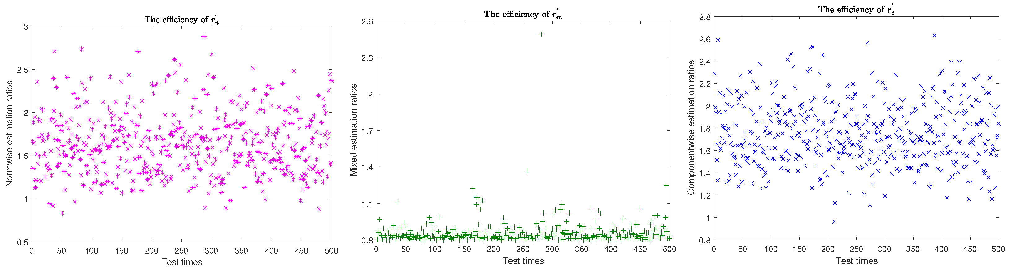
• Estimate the normwise condition number (33) by

  $$\begin{array}{c}\hfill n_{\mathrm{SCE}}^{†}(\mathcal{M},\mathcal{L},\mathcal{K})=\frac{N_{\mathrm{SCE}}^{†}{\parallel [\mathcal{M},\mathcal{L},\mathcal{K}]\parallel }_F}{{∥{\mathcal{K}}_{\mathcal{M}\mathcal{L}}^{†}∥}_F},\end{array}$$

  (40)

  where $N_{\mathrm{SCE}}^{†}:=\frac{{\omega }_q}{{\omega }_p}\sqrt{{∥{\lambda }_1∥}_2^2+{∥{\lambda }_2∥}_2^2+\cdots +{∥{\lambda }_q∥}_2^2}={∥n_{\mathrm{abs}}^{†}∥}_F$.

The corresponding SSCE method, which is from [23] and has been used in numerous problems (see, for example, [27,32,33,34]), is required in order to estimate the mixed and componentwise condition numbers for ${\mathcal{K}}_{\mathcal{M}\mathcal{L}}^{†}$.

Algorithm B (Small-sample statistical condition estimation method for the mixed and componentwise condition numbers of $\mathcal{ML}$-weighted pseudoinverse)

• Generate matrices $\left[\mathit{\delta }{\mathcal{M}}_1,\mathit{\delta }{\mathcal{L}}_1,\mathit{\delta }{\mathcal{K}}_1\right],\left[\mathit{\delta }{\mathcal{M}}_2,\mathit{\delta }{\mathcal{L}}_2,\mathit{\delta }{\mathcal{K}}_2\right],\dots ,\left[\mathit{\delta }{\mathcal{M}}_q,\mathit{\delta }{\mathcal{L}}_q,\mathit{\delta }{\mathcal{K}}_q\right]$ with each entry in $\mathcal{N}(0,1)$ and orthonormalize the following matrix

  $$\left[\begin{array}{cccc}vec\left(\mathit{\delta }{\mathcal{M}}_1\right)& vec\left(\mathit{\delta }{\mathcal{M}}_2\right)& \cdots & vec\left(\mathit{\delta }{\mathcal{M}}_q\right)\\ vec\left(\mathit{\delta }{\mathcal{L}}_1\right)& vec\left(\mathit{\delta }{\mathcal{L}}_2\right)& \cdots & vec\left(\mathit{\delta }{\mathcal{L}}_q\right)\\ vec\left(\mathit{\delta }{\mathcal{K}}_1\right)& vec\left(\mathit{\delta }{\mathcal{K}}_2\right)& \cdots & vec\left(\mathit{\delta }{\mathcal{K}}_q\right)\end{array}\right]$$

  to obtain $\left[{\tau }_1,{\tau }_2,\dots ,{\tau }_q\right]$ by modified Gram-Schmidt orthogonalization process. Each ${\tau }_i$ can be converted into the corresponding matrices $\left[\mathit{\delta }{\mathcal{M}}_i,\mathit{\delta }{\mathcal{L}}_i,\mathit{\delta }{\mathcal{K}}_i\right]$ by applying the unvec operation. Let $\left[\mathit{\delta }{\mathcal{M}}_i,\mathit{\delta }{\mathcal{L}}_i,\mathit{\delta }{\mathcal{K}}_i\right]$ be the matrix $\left[\widetilde{\mathit{\delta }{\mathcal{M}}_i},\widetilde{\mathit{\delta }{\mathcal{L}}_i},\widetilde{\mathit{\delta }{\mathcal{K}}_i}\right]$ multiplied by $[\mathcal{M},\mathcal{L},\mathcal{K}]$ componentwise.
• Let $p=mn+ms+ln$. Approximate ${\omega }_p$ and ${\omega }_q$ by (38).
• For $\alpha =1,2,\dots ,q,$ calculate ${\lambda }_{\alpha }$ by (39). Compute the absolute condition vector

  $$n_{\mathrm{SCE}}^{†}=\frac{{\omega }_q}{{\omega }_p}\sqrt{{\left|{\lambda }_1\right|}^2+{\left|{\lambda }_2\right|}^2+\cdots +{\left|{\lambda }_q\right|}^2}$$
• Estimate the mixed and componentwise condition estimations $m_{sce}^{†}(\mathcal{M},\mathcal{L},\mathcal{K})$ and $c_{sce}^{†}(\mathcal{M},\mathcal{L},\mathcal{K})$ as follows:

  $$m_{\mathrm{SCE}}^{†}(\mathcal{M},\mathcal{L},\mathcal{K})=\frac{\parallel n_{\mathrm{SCE}}^{†}{\parallel }_{\infty }}{\parallel \mathrm{vec}\left({\mathcal{K}}_{\mathcal{M}\mathcal{L}}^{†}\right){\parallel }_{\infty }},c_{\mathrm{SCE}}^{†}(\mathcal{M},\mathcal{L},\mathcal{K})={∥\frac{n_{\mathrm{SCE}}^{†}}{\mathrm{vec}\left({\mathcal{K}}_{\mathcal{M}\mathcal{L}}^{†}\right)}∥}_{\infty }.$$

In order to estimate the normwise, mixed, and componentwise condition numbers of the $\mathcal{ML}$-WLS problem, we provide Algorithm C based on the SSCE approach [23].

Algorithm C (Small-sample statistical condition estimation method for the condition numbers of $\mathcal{ML}$-weighted least squares problem)

• Generate matrices $\left[\mathit{\delta }{\mathcal{M}}_1,\mathit{\delta }{\mathcal{L}}_1,\mathit{\delta }{\mathcal{K}}_1,\mathit{\delta }{h}_1\right],\left[\mathit{\delta }{\mathcal{M}}_2,\mathit{\delta }{\mathcal{L}}_2,\mathit{\delta }{\mathcal{K}}_2,\mathit{\delta }{h}_2\right],\dots ,\left[\mathit{\delta }{\mathcal{M}}_t,\mathit{\delta }{\mathcal{L}}_t,\mathit{\delta }{\mathcal{K}}_t,\mathit{\delta }{h}_t\right]$ with entries in $\mathcal{N}(0,1),$ where $h_i\in {\mathbb{R}}^m.$ To orthonormalize the below matrix

  $$\left[\begin{array}{cccc}vec\left(\mathit{\delta }{\mathcal{M}}_1\right)& vec\left(\mathit{\delta }{\mathcal{M}}_2\right)& \cdots & vec\left(\mathit{\delta }{\mathcal{M}}_t\right)\\ vec\left(\mathit{\delta }{\mathcal{L}}_1\right)& vec\left(\mathit{\delta }{\mathcal{L}}_2\right)& \cdots & vec\left(\mathit{\delta }{\mathcal{L}}_t\right)\\ vec\left(\mathit{\delta }{\mathcal{K}}_1\right)& vec\left(\mathit{\delta }{\mathcal{K}}_2\right)& \cdots & vec\left(\mathit{\delta }{\mathcal{K}}_t\right)\\ \mathit{\delta }{h}_1& \mathit{\delta }{h}_2& \cdots & \mathit{\delta }{h}_t\end{array}\right]$$

  to obtain an orthonormal matrix $\left[{\xi }_1,{\xi }_2,\dots ,{\xi }_t\right],$ by using modified Gram-Schmidt orthogonalization technique. Where ${\xi }_i$ can be converted into the corresponding matrices $\left[\mathit{\delta }{\mathcal{M}}_i,\mathit{\delta }{\mathcal{L}}_i,\mathit{\delta }{\mathcal{K}}_i,\mathit{\delta }{h}_i\right]$ by applying the unvec operation.
• Let $\alpha =mn+sm+ln+m$. Approximate ${\omega }_p$ and ${\omega }_t$ by using (38).
• For $j=1,2,\dots ,t,$ compute $y_j$ from (31)

  $$\begin{array}{cc}\hfill y_j& ={\mathcal{R}}^{†}\mathit{\delta }{\mathcal{M}}_{j}r-{\mathcal{K}}_{\mathcal{M}\mathcal{L}}^{†}\mathit{\delta }{\mathcal{K}}_{j}x-{\left(\mathcal{L}\mathcal{P}\right)}^{†}\mathit{\delta }{\mathcal{L}}_{j}x-{\mathcal{Q}}^{†}\mathit{\delta }{\mathcal{L}}_j^T\mathcal{L}x\hfill \\ \hfill & +{\mathcal{Q}}^{†}\mathit{\delta }{\mathcal{K}}_j^T{\mathcal{M}}^T{\left(\mathcal{L}{\left(\mathcal{M}\mathcal{K}\right)}^{†}\right)}^T\mathcal{L}x+{\mathcal{Q}}^{†}{\mathcal{K}}^T\mathit{\delta }{\mathcal{M}}_j^T{\left(\mathcal{L}{\left(\mathcal{M}\mathcal{K}\right)}^{†}\right)}^T\mathcal{L}x+{\mathcal{K}}_{\mathcal{M}\mathcal{L}}^{†}\mathit{\delt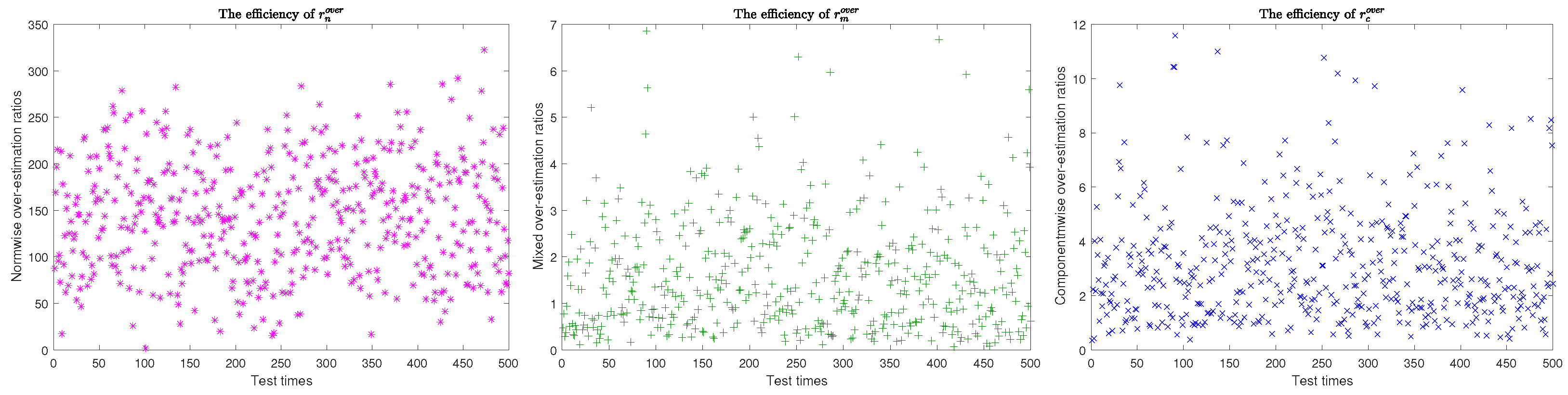a }{h}_j.\hfill \end{array}$$
  Using the approximations for ${\omega }_p$ and ${\omega }_t$, estimate the absolute condition vector

  $${\kappa }_{abs}^{\mathcal{ML}-WLS}=\frac{{\omega }_t}{{\omega }_p}\sqrt{{\left|y_1\right|}^2+{\left|y_2\right|}^2+\cdots +{\left|y_t\right|}^2}.$$
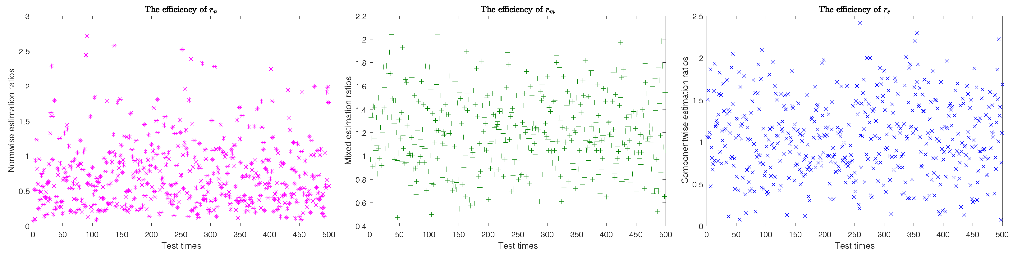
• Estimate the normwise condition estimation as follows:

  $$n_{\mathrm{SCE}}^{\mathcal{ML}-WLS}=\frac{{∥{\kappa }_{abs}^{\mathcal{ML}-WLS}∥}_2{∥{\left[{\mathcal{M}}^T,{\mathcal{L}}^T,{\mathcal{K}}^T,h^T\right]}^T∥}_2}{{\parallel x\parallel }_2}.$$
• Compute the mixed condition estimation $m_{\mathrm{SCE}}$ and componentwise condition estimation $c_{\mathrm{SCE}}$ as follows:

  $$m_{\mathrm{SCE}}:=\frac{{∥{\kappa }_{abs}^{\mathcal{ML}-WLS}∥}_{\infty }}{{\parallel x\parallel }_{\infty }},c_{\mathrm{SCE}}:={∥\frac{{\kappa }_{abs}^{\mathcal{ML}-WLS}}{x}∥}_{\infty }.$$

Next, we provide three individual examples. In the first, we compare our SCE-based estimates with the condition numbers of ${\mathcal{K}}_{\mathcal{M}\mathcal{L}}^{†}$. It also concludes how well Algorithms A and B perform while developing very high estimations. The second one helps to show the accuracy of statistical condition estimators of normwise, mixed, and componentwise condition numbers for the $\mathcal{ML}$-WLS solution. The third one verifies the effectiveness of over-estimation ratios by Algorithm C related to the condition numbers of the $\mathcal{ML}$-WLS solution.

Example 1.

We constructed 200 matrices by repeatedly applying the data matrices $\mathcal{K},\mathcal{M},and\mathcal{L}$ below and varying the value of θ.

$$\mathcal{K}=\left[\begin{array}{cccc}sin\theta & 0& \dots & 0\\ 0& \theta & \dots & 0\\ ⋮& ⋮& \ddots & ⋮\\ 0& 0& \dots & \theta -3\\ 0& 0& \dots & cos\theta \end{array}\right]\in {\mathbb{R}}^{m\times n},\mathcal{M}=\left[\begin{array}{ccccc}2& 0& 0& \dots & 0\\ 0& cos\theta & 0& \dots & 0\\ 0& 0& 1& \dots & 0\\ ⋮& ⋮& ⋮& \ddots & ⋮\\ 0& 0& 0& \dots & \theta \end{array}\right]\in {\mathbb{R}}^{s\times m},\mathcal{L}=\left[\begin{array}{cccc}1& 0& \dots & 0\\ 0& 0& \dots & 0\\ ⋮& ⋮& \ddots & ⋮\\ 0& 0& \dots & {\theta }^2-{10}^{-4}\end{array}\right]\in {\mathbb{R}}^{l\times n},$$

The results in Table 1 show that Algorithms A and B can reliably estimate the condition numbers in the majority of instances. As stated in ([35], Chapter 15), an estimate of the condition number that is correct to within a factor of 10 is usually suitable because it is the magnitude of an error bound that is of interest rather than its precise value.

Table 1. The efficiency of statistical condition estimates by Algorithms A and B.

$m,n,s,l$	$\theta$	$n_{\mathrm{SCE}}^{†}$	$n^{†}$	$n_{\mathrm{u}}^{†}$	$m_{\mathrm{SCE}}^{†}$	$m^{†}$	$m_{\mathrm{u}}^{†}$	$c_{\mathrm{SCE}}^{†}$	$c^{†}$	$c_{\mathrm{u}}^{†}$
20, 10, 5, 15	$\frac{\pi }{3}$	1.1022e+01	2.7522e+01	5.7654e+02	3.1027e+00	5.3832e+00	5.2416e+01	4.2054e+00	5.4372e+00	6.2721e+01
	$\frac{\pi }{4}$	2.2053e+01	3.2618e+01	7.1865e+02	2.3128e+00	3.4752e+00	2.3096e+01	2.5062e+00	3.6543e+00	3.6092e+01
	$\frac{\pi }{5}$	3.1054e+01	4.2065e+01	2.6211.e+03	2.5201e+00	3.7032e+00	3.1965e+02	2.7084e+00	3.8033e+00	4.0544e+02
	$\frac{\pi }{6}$	3.1054e+01	4.2065e+01	2.6211.e+03	2.5201e+00	3.7032e+00	3.1965e+02	2.7084e+00	3.8033e+00	4.0544e+02
$m,n,s,l$	$\theta$	$n_{\mathrm{SCE}}^{†}$	$n^{†}$	$n_{\mathrm{u}}^{†}$	$m_{\mathrm{SCE}}^{†}$	$m^{†}$	$m_{\mathrm{u}}^{†}$	$c_{\mathrm{SCE}}^{†}$	$c^{†}$	$c_{\mathrm{u}}^{†}$
60, 40, 30, 50	$\frac{\pi }{3}$	4.4034e+01	5.6652e+01	5.1977e+03	3.8402e+00	6.0328e+00	8.6047e+01	5.1054e+00	7.3590e+00	8.9076e+01
	$\frac{\pi }{4}$	4.7901e+01	5.9084e+01	7.4710e+03	2.8033e+00	3.2228e+00	6.3722e+01	3.1560e+00	4.3805e+00	7.6943e+01
	$\frac{\pi }{5}$	2.1642e+02	3.7611e+02	1.3179e+04	2.8764e+00	4.3502e+00	4.0644e+02	4.1232e+00	5.4653e+00	5.3772e+02
	$\frac{\pi }{6}$	2.1642e+02	3.7611e+02	1.3179e+04	2.8764e+00	4.3502e+00	4.0644e+02	4.1232e+00	5.4653e+00	5.3772e+02
$m,n,s,l$	$\theta$	$n_{\mathrm{SCE}}^{†}$	$n^{†}$	$n_{\mathrm{u}}^{†}$	$m_{\mathrm{SCE}}^{†}$	$m^{†}$	$m_{\mathrm{u}}^{†}$	$c_{\mathrm{SCE}}^{†}$	$c^{†}$	$c_{\mathrm{u}}^{†}$
100, 60, 40, 80	$\frac{\pi }{3}$	1.6543e+02	2.4638e+02	3.0643e+04	4.3222e+00	6.1108e+00	4.0644e+02	5.7642e+00	7.4544e+00	5.3632e+02
	$\frac{\pi }{4}$	1.2324e+02	2.3207e+02	4.2501e+04	3.6233e+00	5.2326e+00	2.5489e+02	5.3562e+00	6.6533e+00	3.6471e+02
	$\frac{\pi }{5}$	2.5434e+02	3.2455e+02	6.5731e+04	3.2064e+00	4.5211e+00	5.7654e+02	4.8659e+00	5.7532e+00	6.5703e+02
	$\frac{\pi }{6}$	2.5434e+02	3.2455e+02	6.5731e+04	3.2064e+00	4.5211e+00	5.7654e+02	4.8659e+00	5.7532e+00	6.5703e+02
$m,n,s,l$	$\theta$	$n_{\mathrm{SCE}}^{†}$	$n^{†}$	$n_{\mathrm{u}}^{†}$	$m_{\mathrm{SCE}}^{†}$	$m^{†}$	$m_{\mathrm{u}}^{†}$	$c_{\mathrm{SCE}}^{†}$	$c^{†}$	$c_{\mathrm{u}}^{†}$
200, 100, 50, 150	$\frac{\pi }{3}$	2.0331e+02	4.2224e+02	7.1023e+04	4.7532e+00	7.0665e+00	3.2052e+03	6.7051e+00	7.8066e+00	4.6281e+03
	$\frac{\pi }{4}$	2.2053e+02	3.2618e+02	7.4533e+04	4.1054e+00	6.2350e+00	1.2411e+03	6.0462e+00	7.1102e+00	2.7403e+03
	$\frac{\pi }{5}$	4.1326e+02	6.7651e+02	9.2016e+04	3.6325e+00	5.3824e+00	4.5341e+03	5.1632e+00	6.5032e+00	7.2305e+03
	$\frac{\pi }{6}$	4.1326e+02	6.7651e+02	9.2016e+04	3.6325e+00	5.3824e+00	4.53414e+03	5.1632e+00	6.5032e+00	7.2305e+03

Figure 1 demonstrates that Algorithms A and B are very efficient in estimating condition numbers of ${\mathcal{K}}_{\mathcal{M}\mathcal{L}}^{†}$. To evaluate the efficiency of the Algorithms A and B, we created 500 matrix pairings and set $m=300$, $n=150$, $s=100$, $l=200$ and $q=3$ with fixed $\theta =\frac{\pi }{6}$. In order to determine the effectiveness of Algorithms A and B, we specify the following ratios:

$$\begin{array}{c}\hfill r_s^{\prime }=\frac{n_{\mathrm{SCE}}^{†}}{n^{†}},r_m^{\prime }=\frac{m_{\mathrm{SCE}}^{†}}{m^{†}},r_c^{\prime }=\frac{c_{\mathrm{SCE}}^{†}}{c^{†}}.\end{array}$$

Figure 1. Efficiency of condition eliminators of Algorithms A and B.

Example 2.

The nonsymmetric Gaussian random Toeplitz matrix ${\mathcal{L}}_1$ is constructed using the Matlab function $\mathrm{toeplitz}(\mathrm{c},\mathrm{r})$ using $c=randn(s,1)$ and $r=randn(s,1)$, where $\mathcal{L}=[{\mathcal{L}}_1,0]$. Assume that $Y\in {\mathbb{R}}^{m\times n}$ and $U\in {\mathbb{R}}^{m\times n}$ are the random orthogonal matrices, and $\Gamma$ is the diagonal matrix with a certain condition number and positive elements on its diagonal. Following that, we are given the matrices $\mathcal{K}$ and $\mathcal{M}$ as

$$\mathcal{K}={\mathcal{M}}^{\frac{1}{2}}Z\left[\begin{array}{c}\mathsf{{\rm Y}}\hfill \\ 0\hfill \end{array}\right]Y^T,Z=U{\Gamma }^{-\frac{1}{2}},\mathcal{M}=U\Gamma U^T,$$

where $\mathsf{{\rm Y}}=n^{-1}diag(n^l,(n-1)l,\dots ,1)$. The residual vector $r=h-\mathcal{K}x={\mathcal{M}}^{\frac{1}{2}}Z\left[\begin{array}{c}0\hfill \\ \upsilon \hfill \end{array}\right]$ and the solution $x={(1,2^2,\dots ,n^2)}^T$ with $\upsilon \in {\mathbb{R}}^{m-n}$ indicating any random vector with a certain norm and $h={\mathcal{M}}^{-\frac{1}{2}}Z\left[\begin{array}{c}0\hfill \\ \upsilon \hfill \end{array}\right]+{\mathcal{M}}^{\frac{1}{2}}Z\left[\begin{array}{c}\mathsf{{\rm Y}}{Y}^{T}x\hfill \\ 0\hfill \end{array}\right]$. Here, we construct 200 random $\mathcal{ML}$-WLS problems for each specified $cond\left(\mathcal{K}\right)=n^l$ to check the performance of Algorithm C.

The mixed and componentwise condition numbers, rather than the normwise condition number, are more appropriate for describing the underlying conditioning of this $\mathcal{ML}$-WLS problem, considering the facts given in Table 2. Furthermore, we observed that condition estimates based on SSCE may yield accurate results when executed by Algorithm C.

Table 2. The efficiency of statistical condition estimates by Algorithm C.

$m,n,s,l$	$n^l$	$n_{\mathrm{SCE}}^{\mathcal{ML}-WLS}$	$n^{\mathcal{ML}-WLS}$	$n^{upper}$	$m_{\mathrm{SCE}}^{\mathcal{ML}-WLS}$	$m^{\mathcal{ML}-WLS}$	$m^{upper}$	$c_{\mathrm{SCE}}^{\mathcal{ML}-WLS}$	$c^{\mathcal{ML}-WLS}$	$c^{upper}$
30, 20, 10, 15	${10}^0$	1.5301e+01	3.3711e+01	4.3502e+03	3.1081e+00	4.5121e+00	1.7609e+02	4.1428e+00	5.1213e+00	2.3461e+02
	${10}^{-1}$	3.7103e+03	4.1046e+03	1.2353e+05	4.1311e+00	5.4115e+00	3.0554e+02	5.4401e+00	6.5041e+00	4.5530e+02
	${10}^{-2}$	4.0511e+03	5.6105e+03	1.8619e+05	4.1781e+00	5.5733e+00	3.6102e+02	5.6505e+00	6.7504e+00	4.7082e+02
	${10}^{-4}$	5.0171e+03	6.4115e+03	5.4632e+05	5.3161e+00	6.4132e+00	4.3011e+02	6.1865e+00	7.1805e+00	5.0122e+02
	${10}^{-7}$	6.3304e+04	7.8651e+04	5.7011e+05	6.6701e+00	7.3101e+00	4.6750e+02	7.5311e+00	7.6541e+00	5.3443e+02
$m,n,s,l$	$n^l$	$n_{\mathrm{SCE}}^{\mathcal{ML}-WLS}$	$n^{\mathcal{ML}-WLS}$	$n^{upper}$	$m_{\mathrm{SCE}}^{\mathcal{ML}-WLS}$	$m^{\mathcal{ML}-WLS}$	$m^{upper}$	$c_{\mathrm{SCE}}^{\mathcal{ML}-WLS}$	$c^{\mathcal{ML}-WLS}$	$c^{upper}$
90, 60, 30, 45	${10}^0$	4.0314e+01	5.1011e+01	5.0754e+03	3.1011e+00	4.1041e+00	6.3560e+02	4.1566e+00	5.1108e+00	9.8642e+02
	${10}^{-1}$	1.1135e+03	3.1103e+03	3.1398e+05	3.3671e+00	4.5781e+00	1.4567e+03	4.1401e+00	5.0713e+00	3.5567e+03
	${10}^{-2}$	4.5311e+03	5.7611e+03	3.5743e+05	3.4122e+00	4.7551e+00	1.6091e+03	4.4311e+00	5.7141e+00	3.8110e+03
	${10}^{-4}$	6.1351e+03	7.3450e+03	6.5865e+05	4.0167e+00	5.3502e+00	2.4113e+03	5.1104e+00	6.0511e+00	4.5225e+03
	${10}^{-7}$	3.6111e+04	4.7661e+04	6.8952e+05	4.6311e+00	5.6215e+00	2.7840e+03	5.3054e+00	6.4403e+00	4.8203e+03
$m,n,s,l$	$n^l$	$n_{\mathrm{SCE}}^{\mathcal{ML}-WLS}$	$n^{\mathcal{ML}-WLS}$	$n^{upper}$	$m_{\mathrm{SCE}}^{\mathcal{ML}-WLS}$	$m^{\mathcal{ML}-WLS}$	$m^{upper}$	$c_{\mathrm{SCE}}^{\mathcal{ML}-WLS}$	$c^{\mathcal{ML}-WLS}$	$c^{upper}$
120, 80, 40, 60	${10}^0$	3.3401e+01	4.5611e+01	7.1209e+03	1.7101e+00	3.8115e+00	8.3411e+02	3.6411e+00	4.7110e+00	9.7438e+03
	${10}^{-1}$	1.7611e+03	1.1403e+03	6.3689e+05	1.4471e+00	1.5171e+00	3.4229e+03	1.3544e+00	3.4811e+00	6.0431e+03
	${10}^{-2}$	3.4511e+03	5.0411e+03	6.7754e+05	1.6331e+00	1.7813e+00	3.9810e+03	3.5886e+00	4.7805e+00	6.4332e+03
	${10}^{-4}$	5.1014e+03	6.1331e+03	8.2306e+05	1.8041e+00	1.8866e+00	5.4240e+03	4.0113e+00	5.1531e+00	7.3552e+03
	${10}^{-7}$	1.7411e+04	3.3811e+04	8.6435e+05	3.7316e+00	4.8031e+00	5.6708e+03	4.1108e+00	5.8611e+00	7.6622e+03
$m,n,s,l$	$n^l$	$n_{\mathrm{SCE}}^{\mathcal{ML}-WLS}$	$n^{\mathcal{ML}-WLS}$	$n^{upper}$	$m_{\mathrm{SCE}}^{\mathcal{ML}-WLS}$	$m^{\mathcal{ML}-WLS}$	$m^{upper}$	$c_{\mathrm{SCE}}^{\mathcal{ML}-WLS}$	$c^{\mathcal{ML}-WLS}$	$c^{upper}$
150, 100, 50, 75	${10}^0$	3.1517e+01	4.3401e+01	9.0654e+03	1.5113e+00	3.6305e+00	4.7622e+03	3.1077e+00	4.1765e+00	5.1108e+03
	${10}^{-1}$	1.6311e+03	1.1451e+03	8.6422e+05	1.1411e+00	1.4134e+00	6.3005e+03	1.1711e+00	3.3086e+00	8.5994e+03
	${10}^{-2}$	3.0558e+03	4.7550e+03	8.8043e+05	1.4770e+00	1.6511e+00	6.9021e+03	3.1341e+00	4.5311e+00	8.7043e+03
	${10}^{-4}$	5.0141e+03	5.8301e+03	9.4660e+05	1.0111e+00	1.7001e+00	8.2765e+03	3.7661e+00	5.0111e+00	9.0492e+03
	${10}^{-7}$	1.5431e+04	3.0801e+04	9.7034e+05	3.1314e+00	4.6441e+00	8.8211e+03	4.1055e+00	5.7101e+00	9.8955e+03

The ratios between the exact condition numbers and their estimated values are listed here.

$$\begin{array}{c}\hfill r_s=\frac{n_{\mathrm{SCE}}^{\mathcal{ML}-WLS}}{n^{\mathcal{ML}-WLS}},r_m=\frac{m_{\mathrm{SCE}}^{\mathcal{ML}-WLS}}{m^{\mathcal{ML}-WLS}},r_c=\frac{c_{\mathrm{SCE}}^{\mathcal{ML}-WLS}}{c^{\mathcal{ML}-WLS}}.\end{array}$$

In order to determine the effectiveness of Algorithm C, generate 500 random $\mathcal{ML}$-WLS problems with the assumptions that $m=200$, $n=100$, $l=150$, and $s=50$ and we used the parameter $t=2$. Therefore, as seen in Figure 2, normwise condition estimation, $r_n$, is not as effective as mixed condition estimation, $r_m$, and componentwise condition estimation, $r_c$.

Figure 2. Efficiency of condition eliminators of Algorithm C.

Example 3.

Consider the random orthogonal matrices: $U\in {\mathbb{R}}^{s\times s}$, $V\in {\mathbb{R}}^{l\times l}$, $Y\in {\mathbb{R}}^{m\times m}$, $Z\in {\mathbb{R}}^{n\times n}$ then the matrices $\mathcal{K}$, $\mathcal{M}$, and $\mathcal{L}$ are provided by

$$\mathcal{K}=Y^{-1}{\Lambda }_{\mathcal{K}}{Z}^T,\mathcal{L}=V{\Lambda }_{\mathcal{L}}^{-\frac{1}{2}}{Z}^T,\mathcal{M}=U{\Lambda }_{\mathcal{M}}{Y}^T,$$

with appropriate sizes, where ${\Lambda }_{\mathcal{K}}\in {\mathbb{R}}^{m\times n}$, ${\Lambda }_{\mathcal{M}}\in {\mathbb{R}}^{s\times m}$ and ${\Lambda }_{\mathcal{L}}\in {\mathbb{R}}^{l\times n}$ are diagonal matrices with diagonal elements distributed exponentially from ${\kappa }_{\mathcal{K}}^{-1}$ to 1. Furthermore, we define $x={\left(1,2^2,\dots ,n^2\right)}^T$ as the solution x and $h=r+{\mathcal{K}}_{\mathcal{M}\mathcal{L}}^{†}x$, where r is the random vector of the 2-norm.

For the perturbations, we generate them as

$$\begin{array}{c}\hfill \mathsf{\Delta }\mathcal{K}={\mathit{\epsilon }}_1\times (E\odot \mathcal{K}),\mathsf{\Delta }\mathcal{M}={\mathit{\epsilon }}_1\times (F\odot \mathcal{M}),\mathsf{\Delta }\mathcal{L}={\mathit{\epsilon }}_1\times (G\odot \mathcal{L}),\mathsf{\Delta }h={\mathit{\epsilon }}_1\times (g\odot h),\end{array}$$

In this example, the componentwise product of two matrices is indicated by ⊙, and the random matrices E, F, G, and g have uniformly distributed components in the open interval $(-1,1)$ and ${\mathit{\epsilon }}_1={10}^{-7}$.

To evaluate the accuracy of the estimators, we define the overestimation ratios.

$$\begin{array}{c}\hfill r_s^{over}:=\frac{n_{\mathrm{SCE}}^{\mathcal{ML}-WLS}·{\mathit{\epsilon }}_1}{{\parallel \mathit{\delta }x\parallel }_2/{\parallel x\parallel }_2},r_m^{over}:=\frac{m_{\mathrm{SCE}}^{\mathcal{ML}-WLS}·{\mathit{\epsilon }}_1}{{\parallel \mathit{\delta }x\parallel }_{\infty }/{\parallel x\parallel }_{\infty }},r_c^{over}:=\frac{c_{\mathrm{SCE}}^{\mathcal{ML}-WLS}·{\mathit{\epsilon }}_1}{{\parallel \mathit{\delta }x/x\parallel }_{\infty }}.\end{array}$$

To check the performance of Algorithm C, we constructed 500 random $\mathcal{ML}$-WLS problems with $m=350$, $s=50$, $l=250$, and $n=150$, and we used the parameter $t=3$ and outputs $n_{\mathrm{SCE}}^{\mathcal{ML}-WLS}$, $m_{\mathrm{SCE}}^{\mathcal{ML}-WLS}$, and $c_{\mathrm{SCE}}^{\mathcal{ML}-WLS}$ of Algorithm C. Figure 3 illustrates that the mixed condition estimation, $r_m^{over}$, and the componentwise condition estimation, $r_c^{over}$, are more efficient when compared to the normwise condition estimation, $r_n^{over}$. However, it is important to note that the latter tends to significantly overestimate the true relative normwise error.

Figure 3. Efficiency of over-estimation ratios of Algorithm C.

6. Conclusions

This article presents explicit expressions and upper bounds for the normwise, mixed, and componentwise condition numbers of the $\mathcal{ML}$-weighted pseudoinverse ${\mathcal{K}}_{\mathcal{ML}}^{†}$. In a specific situation, the results for the K-weighted pseudoinverse and Moore-Penrose inverse are also recovered. Additionally, we provide the process of deriving the $\mathcal{ML}$-weighted least squares solution’s condition numbers from the $\mathcal{ML}$-weighted pseudoinverse condition numbers and ${\mathcal{K}}_{\mathcal{ML}}^{†}$ condition numbers. We proposed three algorithms to efficiently estimate the normwise, mixed, and componentwise conditions for the $\mathcal{ML}$-weighted pseudoinverse ${\mathcal{K}}_{\mathcal{ML}}^{†}$ and $\mathcal{ML}$-weighted least squares solutions using the small-sample statistical condition estimation method. Finally, numerical results confirmed the efficacy and accuracy of the algorithms. In the future, we will continue our study on the $\mathcal{ML}$-weighted pseudoinverse.

References

- Nashed, M.Z. Generalized Inverses and Applications: Proceedings of an Advanced Seminar Sponsored by the Mathematics Research Center, The University of Wisconsin-Madison, New York, NY, USA, 8–10 October 1973; Academic Press, Inc.: Cambridge, MA, USA, 1976; pp. 8–10. [Google Scholar]
- Qiao, S.; Wei, Y.; Zhang, X. Computing Time-Varying ML-Weighted Pseudoinverse by the Zhang Neural Networks. Numer. Funct. Anal. Optim. 2020, 41, 1672–1693. [Google Scholar] [CrossRef]
- Eldén, L. A weighted pseudoinverse, generalized singular values, and constrained least squares problems. BIT 1982, 22, 487–502. [Google Scholar] [CrossRef]
- Galba, E.F.; Neka, V.S.; Sergienko, I.V. Weighted pseudoinverses and weighted normal pseudosolutions with singular weights. Comput. Math. Math. Phys. 2009, 49, 1281–1363. [Google Scholar] [CrossRef]
- Rubini, L.; Cancelliere, R.; Gallinari, P.; Grosso, A.; Raiti, A. Computational experience with pseudoinversion-based training of neural networks using random projection matrices. In Artificial Intelligence: Methodology, Systems, and Applications; Gennady, A., Hitzler, P., Krisnadhi, A., Kuznetsov, S.O., Eds.; Springer International Publishing: New York, NY, USA, 2014; pp. 236–245. [Google Scholar]
- Wang, X.; Wei, Y.; Stanimirovic, P.S. Complex neural network models for time-varying Drazin inverse. Neural Comput. 2016, 28, 2790–2824. [Google Scholar] [CrossRef]
- Zivkovic, I.S.; Stanimirovic, P.S.; Wei, Y. Recurrent neural network for computing outer inverse. Neural Comput. 2016, 28, 970–998. [Google Scholar] [CrossRef]
- Wei, M.; Zhang, B. Structures and uniqueness conditions of MK-weighted pseudoinverses. BIT 1994, 34, 437–450. [Google Scholar] [CrossRef]
- Eldén, L. Perturbation theory for the least squares problem with equality constraints. SIAM J. Numer. Anal. 1980, 17, 338–350. [Google Scholar] [CrossRef]
- Björck, Å. Numerical Methods for Least Squares Problems; SIAM: Philadelphia, PA, USA, 1996. [Google Scholar]
- Wei, M. Perturbation theory for rank-deficient equality constrained least squares problem. SIAM J. Numer. Anal. 1992, 29, 1462–1481. [Google Scholar] [CrossRef]
- Cox, A.J.; Higham, N.J. Accuracy and stability of the null space method for solving the equality constrained least squares problem. BIT 1999, 39, 34–50. [Google Scholar] [CrossRef]
- Li, H.; Wang, S. Partial condition number for the equality constrained linear least squares problem. Calcolo 2017, 54, 1121–1146. [Google Scholar] [CrossRef]
- Diao, H. Condition numbers for a linear function of the solution of the linear least squares problem with equality constraints. J. Comput. Appl. Math. 2018, 344, 640–656. [Google Scholar] [CrossRef]
- Björck, Å.; Higham, N.J.; Harikrishna, P. The equality constrained indefinite least squares problem: Theory and algorithms. BIT Numer. Math. 2003, 43, 505–517. [Google Scholar]
- Cucker, F.; Diao, H.; Wei, Y. On mixed and componentwise condition numbers for Moore Penrose inverse and linear least squares problems. Math Comp. 2007, 76, 947–963. [Google Scholar] [CrossRef]
- Wei, M. Algebraic properties of the rank-deficient equality-constrained and weighted least squares problem. Linear Algebra Appl. 1992, 161, 27–43. [Google Scholar] [CrossRef]
- Gulliksson, M.E.; Wedin, P.A.; Wei, Y. Perturbation identities for regularized Tikhonov inverses and weighted pseudoinverses. BIT 2000, 40, 513–523. [Google Scholar] [CrossRef]
- Samar, M.; Li, H.; Wei, Y. Condition numbers for the K-weighted pseudoinverse and their statistical estimation. Linear Multilinear Algebra 2021, 69, 752–770. [Google Scholar] [CrossRef]
- Samar, M.; Zhu, X.; Shakoor, A. Conditioning theory for Generalized inverse and their estimations. Mathematics 2023, 11, 2111. [Google Scholar] [CrossRef]
- Rice, J. A theory of condition. SIAM J. Numer. Anal. 1966, 3, 287–310. [Google Scholar] [CrossRef]
- Gohberg, I.; Koltracht, I. Mixed, componentwise, and structured condition numbers. SIAM J. Matrix Anal. Appl. 1993, 14, 688–704. [Google Scholar] [CrossRef]
- Kenney, C.S.; Laub, A.J. Small-sample statistical condition estimates for general matrix functions. SIAM J. Sci. Comput. 1994, 15, 36–61. [Google Scholar] [CrossRef]
- Xie, Z.; Li, W.; Jin, X. On condition numbers for the canonical generalized polar decomposition of real matrices. Electron. J. Linear Algebra. 2013, 26, 842–857. [Google Scholar] [CrossRef]
- Horn, R.A.; Johnson, C.R. Topics in Matrix Analysis; Cambridge University Press: New York, NY, USA, 1991. [Google Scholar]
- Magnus, J.R.; Neudecker, H. Matrix Differential Calculus with Applications in Statistics and Econometrics, 3rd ed.; John Wiley and Sons: Chichester, NH, USA, 2007. [Google Scholar]
- Diao, H.; Xiang, H.; Wei, Y. Mixed, componentwise condition numbers and small sample statistical condition estimation of Sylvester equations. Numer. Linear Algebra Appl. 2012, 19, 639–654. [Google Scholar] [CrossRef]
- Baboulin, M.; Gratton, S.; Lacroix, R.; Laub, A.J. Statistical estimates for the conditioning of linear least squares problems. Lect. Notes Comput. Sci. 2014, 8384, 124–133. [Google Scholar]
- Samar, M. A condition analysis of the constrained and weighted least squares problem using dual norms and their statistical estimation. Taiwan. J. Math. 2021, 25, 717–741. [Google Scholar] [CrossRef]
- Li, H.; Wang, S. On the partial condition numbers for the indefinite least squares problem. Appl. Numer. Math. 2018, 123, 200–220. [Google Scholar] [CrossRef]
- Samar, M.; Zhu, X. Structured conditioning theory for the total least squares problem with linear equality constraint and their estimation. AIMS Math. 2023, 8, 11350–11372. [Google Scholar] [CrossRef]
- Diao, H.; Wei, Y.; Xie, P. Small sample statistical condition estimation for the total least squares problem. Numer. Algor. 2017, 75, 435–455. [Google Scholar] [CrossRef]
- Samar, M.; Lin, F. Perturbation and condition numbers for the Tikhonov regularization of total least squares problem and their statistical estimation. J. Comput. Appl. Math. 2022, 411, 114230. [Google Scholar] [CrossRef]
- Diao, H.; Wei, Y.; Qiao, S. Structured condition numbers of structured Tikhonov regularization problem and their estimations. J. Comput. Appl. Math. 2016, 308, 276–300. [Google Scholar] [CrossRef]
- Higham, N.J. Accuracy and Stability of Numerical Algorithms, 2nd ed.; SIAM: Philadelphia, PA, USA, 2002. [Google Scholar]
Disclaimer/Publisher’s Note: The statements, opinions and data contained in all publications are solely those of the individual author(s) and contributor(s) and not of MDPI and/or the editor(s). MDPI and/or the editor(s) disclaim responsibility for any injury to people or property resulting from any ideas, methods, instructions or products referred to in the content. |
© 2024 by the authors. Licensee MDPI, Basel, Switzerland. This article is an open access article distributed under the terms and conditions of the Creative Commons Attribution (CC BY) license (https://creativecommons.org/licenses/by/4.0/).