Article

A Binary-State Continuous-Time Markov Chain Model for Offshoring and Reshoring

Department of Mathematics “Tullio Levi-Civita”, University of Padova, 35121 Padova, Italy
*
Author to whom correspondence should be addressed.
Axioms 2024, 13(5), 300; https://doi.org/10.3390/axioms13050300
Submission received: 31 March 2024 / Revised: 26 April 2024 / Accepted: 29 April 2024 / Published: 1 May 2024
(This article belongs to the Special Issue Advances in Mathematics: Theory and Applications)

Abstract

:
We present a two-country model (North and South) that describes the phenomenon of offshoring and reshoring. The model is a continuous time-controlled Markov chain with binary states. The main trade-off involves production costs and transaction costs between one country and another. In the first part of this paper, we identify the key parameters of the model: the difference in unit production costs between the two countries considered, the marginal cost of transitioning between countries, and the incentive paid by the North country to all companies that have not relocated at the end of the planning interval. The final goal of our paper is to understand how national tax incentives can influence this process.

1. Introduction

In recent decades, the practice of establishing a business, or part of it, in a different place than the home country has become increasingly popular [1]. This phenomenon, known as offshoring, applies to several sectors, from manufacturing to services [2]. However, in recent years, the global socioeconomic situation has increased the reverse phenomenon: reshoring [3]. Reshoring is a voluntary corporate strategy regarding partial or total relocation of production (insourced or outsourced) in the home country to meet local, regional, or global demands, as defined by [4]. The explanations for this change in direction are numerous and highly different. Among them, there are well-known economic reasons, such as the reduction in the labor cost gap between the home country and the host country or logistics costs, but also planning risks, such as global supply chain risks and the impact of production/delivery time [3,5]. Furthermore, in determining the spread of reshoring, there are problems related to the lack of skilled workers in the host country or the lack of knowledge about the foreign destination. Finally, today, increasing attention is paid to brand value in terms of social responsibility and quality [6]. Therefore, the need to increase customer satisfaction and the built-in effect play a key role in deciding whether to re-establish a business. An aspect that has particularly interested consumers in recent years is the focus on green policies, leading them to prefer products with a low environmental footprint [7].
In our paper, we investigate the conditions under which offshoring and reshoring occur, as well as how a government can influence this process. The purpose of our model is to analyze the economic relationships that exist between essential quantitative variables in the offshoring and reshoring process. For simplicity, we model a situation in which the motivation for reshoring is only related to the presence of national relocation subsidies, which take place at the end of the programming interval. Only one foreign country is taken into account, and offshoring is determined by the lower production costs in that country. The final goal of our paper is to understand the trade-off between offshoring and reshoring phenomena as a function of the national taxation incentives. Moreover, we are also interested in representing the evolution of the proportion of offshored and home-placed businesses.
The paper is organized as follows. In Section 2, we introduce the model and recall the most important results on the theory of controlled Markov processes with binary state, which is the main mathematical tool used in our analysis. In Section 3, we explicitly compute the optimal control of the problem. In Section 4, we describe the evolution of the offshoring process in the absence of government incentives for reshoring, while in Section 5, we study the impact of a tax incentive assigned at the end of the programming interval. Finally, in Section 6, we summarize the results obtained and propose some extensions of the model that may be relevant for further investigation.

2. The Model

2.1. The Microscopic Model

In this paper, we introduce a North-South model (see [8]) in which companies have the flexibility to select their production locations. In [8], the author builds a growth model that focuses on research and development (R&D) activities and examines the relationship between the North and South regions. Specifically, the model investigates how firms producing final goods in the North inherently influence the extent of international outsourcing of intermediate goods to the South. Our paper does not focus on growth models, but rather it analyses how the presence of incentives can drive companies’ decisions to reshore their production. However, we continue to consider only two possible countries to understand which are the essential parameters that favor offshoring and reshoring. We present the N-player game, followed by its formal limit with infinitely many companies. Although our analysis focuses primarily on the limit model, the N-player game serves as its motivating force, giving a clearer understanding of the parameters involved and providing a sort of microfoundation of the model studied. Strictly speaking, our approach does not fit the conventional definition of a game, as it lacks direct interaction among players. However, conceptualizing it as a game is convenient for two reasons. First, it allows us to apply the standard theory of continuous-time finite-state mean-field games [9,10]. Second, this approach facilitates the presentation of a direct extension of the model in Section 5.
Let us assume that N companies sell their product in the domestic market (in the North country). We identify each company with the index i = 1 , , N . Let us assume that all these companies have the same programming interval [ 0 , T ] . The instantaneous demand for the product produced by the i-th company in the programming interval is assumed to be constant and equal to δ i > 0 . The selling price for one unit of goods is also assumed to be constant in the same programming interval and equal to π i > 0 . However, the production cost varies depending on whether the i-th company is in the North or in the South country. There are no inventories, so everything that is produced is immediately sold.
The decision to produce in the North or in the South country represents the state variable for each company, and it is denoted by X t i , where t [ 0 , T ] . Therefore, X t i can take two possible values: we set X t i = 1 if, at time t, the company denoted by the index i is producing in the South country; on the other hand, X t i = + 1 if, at time t, it is producing in the North country. Therefore, the state of the i-th company is a binary-state variable, i.e., X t i { 1 , + 1 } , depending on where the production is located. We assume that the unit production cost in the South country for the i-th company is ρ i > 0 , while the production cost in the North country is higher and equal to ρ i + ξ i > 0 , where ξ i > 0 .
To treat this model using finite-state continuous-time Markov chains, it is necessary to assume that each company can control the probability rate of transition from one state to another. In our case, the i-th company can control the probability of changing its state, i.e., transitioning from production in the North country to production in the South country or vice versa. We assume that the i-th company can control the transition rate between one state and another. The higher the transition rate, the greater the probability that the company will change the position of the production plant by moving it from one country to another. In this way, our model falls into what is called a continuous-time Markov decision problem with binary states [11]. In more detail, we assume that the dynamics of the problem can be described as follows.
P X t + h i = X t i | X s 1 , X s N , s t = U t i · h + o ( h ) ,
where U t i = φ i ( t , X t 1 , X t N ) 0 is the control function in feedback form of the i-th company. This function is right-continuous at t and depends on the entire state ( X t 1 , X t N ) of the system at time t. Each company has complete information on the behavior of all others and decides whether to activate its own control, which consists of increasing the transition rate from the current state to the opposite, meaning U t i . In other words, each company decides the probability rate with which it changes the production location from the current state to the opposite one (from North to South or South to North). The activation of this control is costly for the i-th company, and we assume that the activation cost is quadratic, i.e., the instantaneous cost function for the activation of the transition rate is c i ( U t i ) = κ i ( U t i ) 2 / 2 + θ i U t i . The North country perfectly knows that the production cost in the South country is more convenient, and, therefore, in order to limit the phenomenon of offshoring, it proposes an incentive to all companies that, at the end of the programming interval, have their production localized in the North country.
The problem for the i-th company can be formulated as follows:
J i [ U s i ] = E 0 T δ i π i ρ i ξ i 2 ( 1 + X t i ) κ i 2 ( U t i ) 2 θ i U t i d t + γ i 2 ( X T i + 1 ) .
For the reader’s convenience, we introduce Table 1 to describe the instantaneous profit of the i-th company, assuming that U s i = 0 , hence, when the i-th company does not activate its transition rate.
In this model, the objective function of each company is independent of the states of the other companies, making the formulation we just described redundant. However, if the parameters we described depended on the states of the other companies, this approach would be exactly what is necessary to describe the problem. For example, if the final incentive depended on the number of companies that relocated their production, then the parameter γ i would no longer be a constant but a function of the state of all other companies: γ i = γ i ( X T 1 , X T N ) .
Let us highlight the importance of the microscopic view by assuming that there are only two companies on the market and that the North country decides to invest a budget β > 0 . Companies producing in the North country at the end of the programming interval receive the entire or a part of the incentive. More precisely, if both companies produce in the North country at time T, each receives an incentive equal to β / 2 . Otherwise, if only one company produces in the North country at the end of the programming interval, that company receives the full incentive β . Finally, if no company produces in the North country at time T, then the incentive is not spent. In this situation, the i-th player incentive γ i ( X 1 , X 2 ) becomes
γ i ( X T i , X T j ) = β ( X T i + 1 ) / 2 1 + ( X T j + 1 ) / 2 ,
with i , j { 1 , 2 } and i j . Similarly, we can move on from 2 to N companies competing for the same incentive budget, and we compute
γ i ( X T 1 , , X T N ) = β ( X T i + 1 ) / 2 1 + j = 1 , j i N ( X T j + 1 ) / 2 .
In the formula above, the average behavior of the other players is highly relevant. Let us define
m N 1 ( T ) : = j = 1 , j i N X T j N 1 .
Therefore, we can rewrite the i-th player incentive as follows:
γ i ( X T 1 , , X T N ) = β ( X T i + 1 ) / 2 1 + ( N 1 ) ( m N 1 ( T ) + 1 ) / 2 .
This reasoning directly connects the original problem to a mean-field game, wherein the strategic interaction among players is present in the scrap value function. When N goes to infinity, the function m N 1 ( T ) can be well approximated by the empirical mean. In mean-field games with Markov feedback Nash equilibria, this convergence process is a challenging task. Convergence can be achieved by identifying the potential limit points of sequences of N-player Nash equilibria, which serve as solutions, to some extent, of the limit model. This approach tackles the convergence issue in mean-field games (see [12] and the references therein for a clear example of the challenges associated with this type of problem). Although, from a mathematical point of view, this is certainly one of the most interesting situations, it could be complicated to understand the problem without clarifying the economic meaning of the parameters δ i , π i , ρ i , ξ i , κ i , θ i . For this reason, in this work, we limit ourselves to a constant function γ i , which corresponds to a fixed incentive that is assigned to all companies that produce in the North country at time T. This approach allows us to obtain closed-form solutions that would not be possible to achieve with direct interactions among different companies. Nevertheless, we introduce the problem in all its generality to allow for an immediate extension to mean-field game theory of the results described here. The approach of continuous-time Markov chain in optimal decision process is widely used in applications; for a recent paper on this topic, we suggest [13] and the references therein.

2.2. The Macroscopic Model

The microscopic model described above can be solved using the techniques presented in [12]. Unfortunately, the solution to the problem with N companies is not very informative because it requires estimating a very large number of parameters and allows obtaining few quantitative indications that clarify the trade-offs between the parameters. At this point, we prefer to introduce the macroscopic model as the formal limit for N that tends to infinity the microscopic one, assuming that all companies are exchangeable. This approach is standard, but it is not trivial: when the model involves mean-field games, the passage to the limit is not straightforward, and additional equilibria may arise (see, e.g., [12,14]). We are not interested in this situation, and instead, we formalize the problem directly, corresponding to the formal limit for a representative player. In this case, all parameters, which were indexed by “i” before, now become independent of i because companies are considered indistinguishable. Table 2 contains the meaning of the variables and parameters used later on.
It is a very strong simplification, but it allows us to identify the explicit trade-off between the model parameters, a result that cannot be obtained in the microscopic formulation. We reiterate that we follow the structure of mean-field games even though there is no strategic interaction among players in this model. In Section 5, we propose an extension that justifies this approach to the problem. The limit as N goes to + can be obtained at a heuristic level. We expect that the average state obeys a Law of Large Numbers, so it converges to a deterministic limit. The representative agent, whose state is denoted by X t , moves according to the following feedback-controlled dynamics:
P X t + h = X t | X s , s t = U t · h + o ( h ) ,
where U t = φ ( t , X t ) 0 is the feedback control function of the representative company. Please note that X t evolves as a controlled binary-state continuous-time Markov chain with transition rate U t . We can rewrite the representative company’s objective function as follows:
J [ U s ] = E 0 T δ π ρ ξ 2 ( 1 + X t ) κ 2 U t 2 θ U t d t + γ 2 ( 1 + X T ) .
To complete the macroscopic analysis, let us introduce the expected value of a representative company, m t , as
m t = E X t
for t [ 0 , T ] . By definition, m t [ 1 , 1 ] throughout the programming interval. This quantity is very important for the policy planner of the North country, as it can be used to describe the proportion of companies that have offshored their production in the South country. Specifically, if m t = 1 , then at time t, all companies have remained in the North country; if m t = 0 , then half of the companies have offshored their production in the South country; and finally, if m t = 1 , then all companies have moved their production to the South country.
The two main research questions of this paper can now be explicitly formulated:
  • What is the trade-off between offshoring costs (described by parameters κ and θ ) and the different production costs in the two countries (described by parameters ρ and ξ )?
  • How can the North country use the incentives described by the parameter γ to avoid the phenomenon of offshoring, and what is the impact of this type of incentives on the evolution over time of the quantity m t that is related to the proportion of companies that have offshored their production?

3. The HJB Equation and the Evolution of m t

The solution procedure for the stochastic optimal control problem characterized by the objective functional (5), by the motion Equation (4), and by the initial condition X 0 is the same as described in [11]. As usual, X 0 is independent of the evolution (4) of the stochastic process ( X t ) t [ 0 , T ] .
Theorem 1.
The optimal control in feedback form for the representative company is
U t = φ ( t , X t ) = [ z t · X t θ ] + κ .
where the function z t satisfies the following backward ODE:
z ˙ t = ( z t + θ ) 2 2 κ δ ξ z t < θ δ ξ | z t |   θ ( z t θ ) 2 2 κ δ ξ z t > θ
with boundary condition
z T = γ .
Proof of Theorem 1.
We face this stochastic control problem using dynamic programming. This approach is standard in applications of Economics and Finance (see, e.g., [15]). For the stochastic optimal control problem (4) and (5), the value function has the following form:
V ( t , x ) = sup U s 0 E t T δ π ρ ξ 2 ( 1 + X s ) κ 2 U s 2 θ U s d s + γ 2 ( 1 + X T ) | X t = x .
The HJB equation associated with this problem is
t V ( t , x ) + max u 0 u x V ( t , x ) + δ π ρ ξ 2 ( 1 + x ) κ 2 u 2 θ u = 0 V ( T , x ) = γ 2 1 + x ,
where, as usual, x V ( t , x ) : = V ( t , x ) V ( t , x ) is the discrete gradient of the value function. Recalling u 0 , we observe that the function
u u x V ( t , x ) + δ ( π ρ + ξ ( 1 + x ) ) κ u 2 / 2 θ u
is strictly concave with respect to u. Hence, by first-order necessary condition, its global maximum point is the zero of its first derivative u x V ( t , x ) κ u θ , when it lies in the interval [ 0 , + ) ; otherwise, it is equal to 0. This control in feedback form can be written as
u = x V ( t , x ) θ + κ ,
where we recall that a + : = max 0 , a and a : = max 0 , a are the positive and the negative part, respectively. Following [11], we want to obtain a backward ODE from the HJB equation. For this aim, we introduce the auxiliary variable
z t : = x V ( t , 1 ) = V ( t , 1 ) V ( t , 1 ) .
We interpret V ( t , 1 ) as the optimal value obtained when starting at x = 1 at time t, analogously, V ( t , 1 ) . Therefore, V ( t , 1 ) V ( t , 1 ) is the algebraic increment obtained by the transition from the state x = 1 to x = 1 at time t. Since we are taking the maximum in the HJB Equation (11), assuming that the initial state at t is x = 1 , the transition from state x = 1 to x = 1 is convenient whenever z t = V ( t , 1 ) V ( t , 1 ) > 0 .
To obtain the backward ODE, we substitute (12) into the HJB Equation (11) and evaluate the result in both states:
t V ( t , 1 ) = x V ( t , 1 ) θ + κ x V ( t , 1 ) δ π ρ ξ +                  + κ 2 x V ( t , 1 ) θ + κ 2 + θ x V ( t , 1 ) θ + κ
t V ( t , 1 ) = x V ( t , 1 ) θ + κ x V ( t , 1 ) δ π ρ +                 + κ 2 x V ( t , 1 ) θ + κ 2 + θ x V ( t , 1 ) θ + κ .
Let us observe that
x V ( t , 1 ) = V ( t , 1 ) V ( t , 1 ) = x V ( t , 1 ) = z t .
We can recognize the auxiliary variable in the above equations. Therefore,
z ˙ t = t V ( t , 1 ) t V ( t , 1 ) = z t κ z t θ + + z t θ + + 1 2 κ z t θ + 2 z t θ + 2 + θ κ z t θ + z t θ + δ ξ .
Recalling classical relations such as [ a ] + = [ a ] , | a | = [ a ] + + [ a ] and a = [ a ] + [ a ] , we obtain
z ˙ t = ( z t + θ ) κ z t + θ + ( z t θ ) κ z t θ + + 1 2 κ [ z t + θ ] 2 [ z t θ ] + 2 δ ξ .
Now, let us consider the three different cases separately.
  • If z t < θ , then z t + θ < 0 and z t θ < 0 , meaning that [ z t + θ ] = ( z t + θ ) and [ z t θ ] + = 0 . In this case (14) reads
    z ˙ t = ( z t + θ ) 2 2 k δ ξ .
  • If | z t |   θ , then z t + θ > 0 and z t θ < 0 , meaning that [ z t + θ ] = 0 and [ z t θ ] + = 0 . In this case (14) reads
    z ˙ t = δ ξ .
  • If z t > θ , then z t + θ > 0 and z t θ > 0 , meaning that [ z t + θ ] = 0 and [ z t θ ] + = ( z t θ ) . In this case (14) reads
    z ˙ t = ( z t θ ) 2 2 k δ ξ .
Hence,
z ˙ t = ( z t + θ ) 2 2 κ δ ξ z t < θ δ ξ | z t |   θ ( z t θ ) 2 2 κ δ ξ z t > θ .
We observe that Equation (15) is differentiable within the different intervals defined by the marginal cost θ . Moreover, we can write this ODE in the following compact way:
z ˙ t = sgn ( z t ) 2 κ [ | z t | θ ] + 2 δ ξ .
Using the boundary condition for the HJB equation we obtain V ( T , x ) = γ 2 1 + x and the definition of the function z t , it yields
z T = V ( T , 1 ) V ( T , 1 ) = γ .
The optimal control in feedback form is characterized by the following function:
φ ( t , x ) = x V ( t , x ) θ + κ = z t · x θ + κ
since x V ( t , x ) = V ( t , x ) V ( t , x ) , corresponds to z t if x = 1 , to z t if x = 1 .
Now, putting together (15), (17), and (18) we can conclude. □
Theorem 1 identifies the optimal strategy for the representative company. However, the most relevant information for the policymaker is related to the macroscopic evolution of the offshoring phenomenon. This information is related to the temporal evolution of the aggregate variable m t , and in the next result, we characterize the ODE that describes these dynamics.
Theorem 2.
Let us assume that the representative company uses the optimal control φ ( t , X t ) characterized in Theorem 1, hence the evolution of the deterministic variable m t = E ( X t ) is described by the following equation
m ˙ t = sgn ( z t ) κ · [ | z t | θ ] + · ( 1 + sgn ( z t ) · m t ) ,
where the function z t satisfies (8) and (9) and m 0 = E ( X 0 ) .
Proof of Theorem 2.
By definition of m t , m ˙ t = d d t E ( X t ) . Please note that we are computing the expected value of a continuous-time finite-state Markov chain with transition rate U t = φ ( t , X t ) ; then if we apply Dynkin’s formula (see, e.g., [16]), we obtain
m ˙ t = d d t E ( X t ) = E ( x X t · φ ( t , X t ) ) = 2 κ · E ( X t · [ z t X t θ ] + ) ,
where the last equality holds true because x X t = X t ( X t ) = 2 X t and φ ( t , X t ) has been characterized in Theorem 1. Now, using the fact that the state is binary, we can explicitly compute the previous expected value, yielding the following result.
m ˙ t = 2 κ E z t θ + · ( 1 + X t ) 2 z t θ + · ( 1 X t ) 2 = 1 κ z t θ + ( 1 + m t ) z t θ ( 1 m t ) = sgn ( z t ) κ · [ | z t | θ ] + · ( 1 + sgn ( z t ) · m t ) .
We note that the results described in this section hold for any value of the parameter γ . Therefore, we have simultaneously addressed both the case γ = 0 , which means the absence of incentives, and the case γ > 0, indicating the presence of economic support from the North country to the companies that maintain domestic production.

4. Offshoring without Incentives

4.1. Technical Analysis

In this case, we assume that there are no incentives that the North country implements to support domestic production. This assumption corresponds to setting the value γ = 0 in the results obtained in Section 3. The final condition (9) becomes z T = 0 . Let us solve the backward ODE Equation (8). By continuity, there exists ε > 0 such that, for t [ T ε , T ] , there is | z t |   θ . Hence, for every t [ T ε , T ] ,
z ˙ t = δ ξ
and we can solve the following Cauchy problem
z ˙ t = δ ξ z T = 0
as long as | z t |   θ . Therefore,
z t = δ ξ ( T t ) .
This solution holds until | z t |   θ , hence let us define t ¯ using the equation z t ¯ = θ . We obtain
t ¯ = T θ δ ξ .
The variable z t in the last part of the programming interval (that is, for t [ max { t ¯ , 0 } , T ] ), is described by (21). If t ¯ 0 , then this function fully describes the optimal feedback strategy. Otherwise, if t ¯ > 0 , then in the first part of the programming interval [ 0 , t ¯ ) , we solve the following Cauchy problem
z ˙ t = ( z θ ) 2 2 κ δ ξ z t ¯ = θ .
Hence we can obtain that, for all t [ 0 , t ¯ ) ,
z t = θ + 2 δ ξ κ tanh δ ξ 2 κ ( t ¯ t ) .
Using Equations (21) and (23), we can compute the corresponding transition rate. By (7), if t ¯ 0 , then
φ ( t , x ) = δ ξ ( T t ) x θ + κ 0 ,
for every t [ 0 , T ] and for every x { 1 , + 1 } . On the other hand, if t ¯ > 0 , then the transition rate is
φ ( t , x ) = θ ( x 1 ) + 2 δ ξ κ tanh δ ξ 2 κ ( t ¯ t ) x + κ = 2 δ ξ κ tanh δ ξ 2 κ ( t ¯ t ) x = 1 0 x = 1
for t [ 0 , t ¯ ) .
Using this optimal control, we can characterize the evolution of the expected value of the process m t . If t ¯ 0 , then m ˙ t 0 . Therefore, denoted by m 0 , the initial condition of the average distribution, it holds m t m 0 , for all t [ 0 , T ] . On the other hand, if t ¯ > 0 , then
m ˙ t = 2 δ ξ κ tanh δ ξ 2 κ ( t ¯ t ) ( 1 + m t )
for t [ 0 , t ¯ ) , and m t m t ¯ for t [ t ¯ , T ] .

4.2. Interpretation of the Results

First, it is important to note that from (25), the transition rate is active from state + 1 to state 1 only. The unique process that we can describe in this situation is the process of offshoring. Moreover, since the model is introduced on a finite horizon, in the last part of the programming interval, no phenomenon occurs because the marginal cost of transition, described by the parameter θ , is too large and makes it not convenient to take any action since one can benefit from this action for a too short period of time. What changes significantly in the optimal control of the representative company is the positivity of time t ¯ , which effectively represents the presence or absence of the offshoring phenomenon. More specifically, we can say that if t ¯ 0 , then there is no offshoring phenomenon, whereas if t ¯ > 0 , there is relocation to the South country. Therefore, we present a sensitivity analysis with respect to the parameters regarding time t ¯ (Table 3).
We recall that the greater the value of t ¯ , the greater the phenomenon of offshoring. The parameters that increase the value of t ¯ increase the location of production in the South country. The parameters T and δ are related to the production and sales of the representative company. Parameters θ and ξ can be influenced by both the North country and the South country. In the following proposition, we clarify the economic phenomena associated with the modification of these two parameters.
Proposition 1.
The North country can contrast the offshoring process by decreasing the difference between two production costs, which is described by the parameter ξ; a standard way to obtain this result consists of imposing a duty on the goods imported by the South country.
The South country can promote the offshoring process by decreasing the marginal cost of the transition described by the parameter θ; a standard way to obtain this result consists of offering incentives to sustain costs.
Proof of Proposition 1.
Let us consider (22). We notice that t ¯ is positive if and only if
T δ ξ θ > 0
The quantity T δ represents the cumulative demand throughout the programming interval. Therefore, T δ ξ is the net profit that a representative company can obtain by moving production from a North country, where the production cost of a unit of good is ρ + ξ , to the South country, where this production cost is just ρ .
The North country can contrast the offshoring process by decreasing the value of ξ . The standard way to obtain this result is to impose a duty on importation so that the difference between the production cost in the North and the South country decreases (see, e.g., [17,18]).
However, the opposite situation concerns the South country, which aims to increase the offshoring phenomenon to boost the companies producing within its own territory. In this case, the best policy is to offer incentives that reduce the marginal transition cost described by the parameter θ (see, e.g., [19]). □

5. Offshoring and Reshoring in Presence of Relocalization Incentives

5.1. Technical Analysis

Assume now the presence of North country’s incentives for relocalization. We will proceed similarly as before, but here we consider γ > 0 . Since the final condition (9) is z T = γ , we cannot be sure if, near the end of the programming interval, | z t |   θ or z t < θ . Consequently, we solve the backward Equation (8) by considering the two cases separately.

5.1.1. Low Incentives: γ θ

Assume, first, that the incentive parameter γ is lower or equal to the marginal cost for delocalization θ . Then, the analysis is similar to what was carried out in Section 4.1. By Equation (8), there must exist ε > 0 such that, for t [ T ε , T ] , so that | z t |   θ holds. More precisely,
z ˙ t = δ ξ z T = γ
as long as | z t |   θ . The solution to the above Cauchy problem is
z t = δ ξ ( T t ) γ
and it holds until z t ¯ ¯ = θ , i.e., for t [ max ( t ¯ ¯ , 0 ) , T ] , with
t ¯ ¯ = T θ + γ δ ξ .
Equation (28) describes the variable z t near the end of the programming interval. If t ¯ ¯ 0 , then the equation is true for all t [ 0 , T ] . Otherwise, if t ¯ ¯ > 0 , Equation (28) holds for t [ t ¯ , T ] , while in the remaining interval z ( · ) is the same as in (23). So,
z t = θ + 2 δ ξ κ tanh δ ξ 2 κ ( t ¯ t )
for all t [ 0 , t ¯ ¯ ) .
Recalling the transition rate (7), we obtain
φ ( t , x ) 0
for t ¯ ¯ 0 and for every x { 1 , + 1 } . On the other hand, if t ¯ ¯ > 0 , the transition rate is
φ ( t , x ) = 2 δ ξ κ tanh δ ξ 2 κ ( t ¯ ¯ t ) x = 1 0 x = 1
for t [ 0 , t ¯ ¯ ) , and φ ( t , x ) 0 in the remaining interval.
By substituting (28) and (30) into Equation (19), we can also calculate the expected production location. As before, if t ¯ ¯ 0 , then m ˙ t 0 ; therefore, m t m 0 . In contrast, if t ¯ ¯ > 0 , then (26) is valid for t [ 0 , t ¯ ¯ ) and m t m t ¯ ¯ while t [ t ¯ ¯ , T ] .

5.1.2. High Incentives: γ > θ

Let us now consider the incentive parameter γ to be higher than the marginal cost θ to move the production location. Under this assumption, the final condition (9) is such that there must exist ε > 0 such that for t ( T ε , T ] it holds z t < θ . By Equation (8), we are solving the Cauchy problem
z ˙ t = ( z + θ ) 2 2 κ δ ξ z T = γ
as long as z t < θ . Therefore,
z t = θ + 2 δ ξ κ tan δ ξ 2 κ ( T t ) + arctan θ γ 2 δ ξ κ
for t ( max ( t ˜ , 0 ) , T ] , where t ˜ is defined by z t ˜ = θ . We compute the switching time
t ˜ = T 2 κ δ ξ arctan γ θ 2 δ ξ κ .
As before, we can observe different situations depending on the sign of t ˜ . If t ˜ 0 , then z t is defined as in (34) for all t [ 0 , T ] ; otherwise, (34) holds only for t [ t ˜ , T ] , while a different equation has to be considered for t < t ˜ . In the latter case, we enter the region | z t |   θ at t ˜ . In this interval, by (8), it holds
z t = δ ξ ( t ˜ t ) θ
until | z t |   θ , i.e., for t [ max { t ¯ ¯ , 0 } , t ˜ ] , with
t ¯ ¯ = t ˜ 2 θ δ ξ .
Once again, we can distinguish two different cases. If t ¯ ¯ 0 , then (36) holds for all t [ 0 , t ˜ ] , otherwise Equation (36) holds for t [ t ¯ ¯ , t ˜ ] , while z t is defined as in (23) in the remaining interval.
Unlike the previous cases, the analysis of the transition rate highlights here the presence of a reshoring phenomenon. By (7) and (34), we obtain
φ ( t , x ) = 0 x = 1 2 δ ξ κ tanh δ ξ 2 κ ( T t ) + arctan θ γ 2 δ ξ κ x = 1
for t ( max { t ˜ , 0 } , T ] . Moreover, if t ˜ > 0 ,
φ ( t , x ) 0 ,
for t [ max { t ¯ ¯ , 0 } , t ˜ ] and, eventually, if t ¯ ¯ > 0
φ ( t , x ) = 2 δ ξ κ tanh δ ξ 2 κ ( t ¯ ¯ t ) x = 1 0 x = 1
for t [ 0 , t ¯ ¯ ) .
The reshoring phenomenon described in (38) also affects the expected location of production (6). For t ( max { t ˜ , 0 } , T ] , we obtain
m ˙ t = 2 δ ξ κ tan δ ξ 2 κ ( T t ) + arctan θ γ 2 δ ξ κ ( 1 m t ) .
If t ˜ > 0 , then m ˙ t 0 for t [ max { t ¯ ¯ , 0 } , t ˜ ] . Furthermore, if t ¯ ¯ > 0 , then
m ˙ t = 2 δ ξ κ tanh δ ξ 2 κ ( t ¯ ¯ t ) ( 1 + m t ) .
for t [ 0 , t ¯ ¯ ) .

5.2. Interpretation of the Results

In contrast to what is observed in Section 4.2, Equation (38) shows an active transition rate from state 1 to state + 1 . As a consequence, in the presence of incentives, a reshoring process can take place. As we shall see later, the fundamental difference compared to the solutions described in Section 4 concerns the presence of the parameter γ : if this quantity is sufficiently large, then our model also describes the phenomenon of reshoring. However, also in this situation, an offshoring phenomenon could occur if the programming interval is long enough or incentives are too low, as described by Equations (40) and (32), respectively. Once again, both cases analyzed illustrate the presence of an interval where no phenomenon occurs. This happens because of the marginal cost of transition θ , which may make it difficult to take any action for too short a period of time. In this second case, the switching times t ¯ ¯ and t ˜ also play a fundamental role in the optimal control of the representative company. Thus, we can summarize here by saying that if incentives are too low, then an offshoring phenomenon may occur when t ¯ ¯ > 0 . Otherwise, an offshoring phenomenon takes place if t ¯ ¯ > 0 , but relocalization to the North country is always present near the end of the programming interval. We also observe that when γ > θ , the starting time of the relocation to the North country t ˜ depends decreasingly on the incentive parameter γ . In fact, the greater the incentives γ , the wider the interval to bring back production to the North country. Similarly, the end of the eventual offshoring interval t ¯ ¯ is decreasing in γ ; hence, the higher the incentives, the narrower the delocalization to the South country. For t ¯ ¯ , the same observation holds for low incentive values, i.e., when γ θ . Given the dependence of the change in production location on the switching times, we present a sensitivity analysis regarding time t ¯ ¯ and t ˜ (Table 4).
We recall that the greater t ¯ ¯ , the long-lasting the offshoring phenomenon; the greater t ˜ , the shorter the relocalization to the North country. All parameters that positively affect t ¯ ¯ increase the location of production in the South country. Those parameters that positively affect t ˜ increase the relocalization to the North country. In particular, a higher cost to relocate the production location θ always corresponds to more limited offshoring and reshoring phenomena. In contrast, higher incentive values γ imply a reduction of the outsourcing interval and an increase in relocation phenomena. The other parameters have a negative effect on the production location by increasing the transfer to the South and limiting the relocation to the North country. We can summarize all this information in the following proposition:
Proposition 2.
The incentives paid by the North country allow the achievement of a reshoring phenomenon from the South country to the North country if and only if these incentives (described by the parameter γ) are greater than the marginal transition cost (described by the parameter θ).
Proof of Proposition 2.
If γ θ , then the optimal control in feedback form is described by Formula (32), hence only offshoring is allowed. On the other hand, if γ > θ then, at the end of the programming interval, the optimal control in feedback form is described by Formula (38), hence the representative company moves its production from South to North in order to obtain the incentives. □
Figure 1 summarizes all the results obtained in both Section 4 and Section 5. In the figure, we include two values of γ to describe their possible mutual positions with respect to the variable θ . The higher dashed blue line corresponds to γ θ , while the lower red one corresponds to γ > θ . We can describe in detail the various behaviors as a function of the value of the function z.
In this case, there is no offshoring because the marginal cost is greater than the savings obtained from production costs; see Equation (24).
Initially, the offshoring phenomenon is present, but it stops in the second part of the programming interval because the savings in production no longer justify the transaction cost; see Equation (25).
Even in the presence of incentives from the North country, there is neither offshoring nor reshoring because the transaction costs are too high compared to other parameters; see Equation (31).
In this situation, incentives from the North country are too weak, and only the offshoring phenomenon occurs in the first part of the programming interval; see Equation (32).
The presence of incentives from the North country is sufficiently intense to allow the reshoring phenomenon in the last part of the programming interval (eventually, in the whole programming interval if t ˜ 0 ). See Equation (38).
This is the most informative situation: offshoring occurs in the first part of the programming interval when there is enough time to take advantage of the low production costs in the South country; reshoring, on the other hand, occurs at the end of the programming interval and is stimulated by sufficiently high incentives paid by the North country; see Equations (38)–(40).
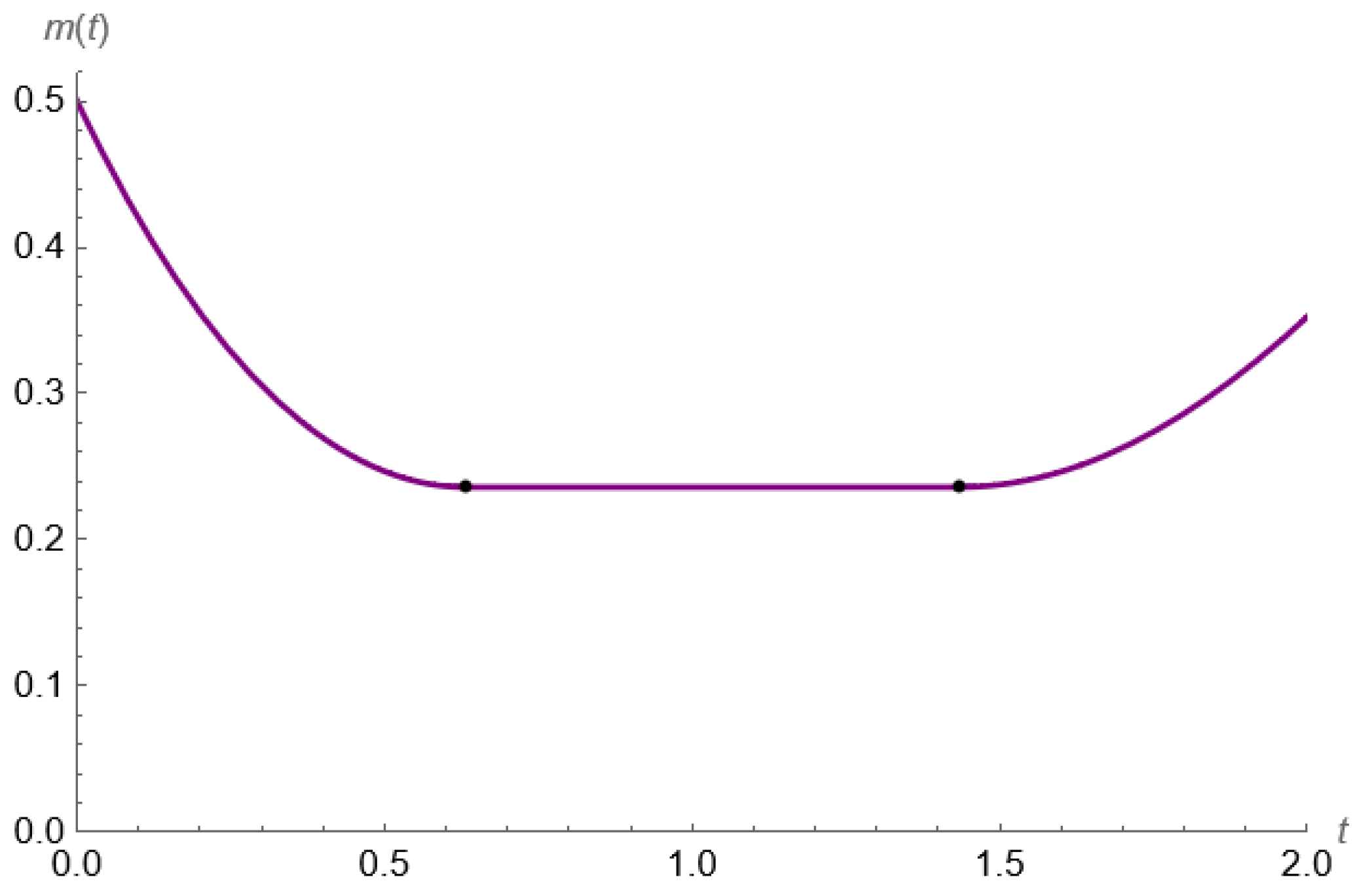
Starting from the most interesting situation (point 6 of the previous list), we numerically solved the differential Equation (19) describing the evolution of the mean of the stochastic process X t . The expected production location m t shown in Figure 2 allows us to visually understand the problem. In this image, the programming interval can be separated into three different parts. The left section, ending at t ¯ ¯ (corresponding to the first black point), shows a decreasing expected production location, which means that an offshoring phenomenon is occurring. The central section is characterized instead by a flat value. This corresponds to the interval of time where no actions occur. On the right, starting at t ˜ , we can observe an increasing trend implied by the reshoring phenomenon.

6. Conclusions

In this work, we have presented a two-country model (North and South) that describes the phenomenon of offshoring and reshoring. From a mathematical point of view, the model is a continuous time-controlled Markov chain with a binary state.
In the first part of this paper, we have identified the parameter values for which the offshoring phenomenon occurs. We have found results well known in the literature: the main trade-off involves production costs and transaction costs between one country and another [18].
In the second part of this work, we hypothesized that the country with higher production costs could counteract the offshoring phenomenon using incentives paid at the end of the planning interval to all companies that have not relocated their production. The most informative solution we obtain can be described as follows: a company initially relocates to take advantage of lower production costs, and only at the end of the planning interval does it use a reshoring policy to benefit from the incentives. The key parameters identified by our model are three: the difference in unit production costs between the two countries considered, the marginal cost of transitioning between countries, and the incentive paid by the North country to companies that have not relocated at the end of the planning interval.
The purpose of this work is to introduce a new model and identify the main trade-offs among the various parameters of the problem. The main extension that makes this problem very interesting both from an economic and mathematical point of view is the dependence of one parameter on the average behavior of the companies. For example, it can be hypothesized that the parameter γ (representing incentives) depends on the number of companies that have relocated: the higher this average, the higher the incentives. This modification turns the problem into a mean-field game (see [20] for an interesting application of mean-field game theory), which is difficult to treat but very rich in terms of information. This entire paper is structured to make this extension very easy and to allow for the easy extension of the research presented in this work to even more detailed and informative situations.

Author Contributions

Conceptualization, C.B., L.G. and E.S.; methodology, C.B., L.G. and E.S.; software, C.B., L.G. and E.S.; formal analysis, C.B., L.G. and E.S.; writing—original draft preparation, C.B., L.G. and E.S.; writing—review and editing, C.B., L.G. and E.S. All authors have read and agreed to the published version of the manuscript.

Funding

This research received no external funding.

Data Availability Statement

Data are contained within the article.

Acknowledgments

We are deeply grateful to the Referees for generously dedicating their time, expertise, and thoughtful feedback to this paper, significantly enhancing its quality and impact.

Conflicts of Interest

The authors declare no conflict of interest.

References

  1. Schwörer, T. Offshoring, domestic outsourcing and productivity: Evidence for a number of European countries. Rev. World Econ. 2013, 149, 131–149. [Google Scholar] [CrossRef]
  2. Metters, R.; Verma, R. History of offshoring knowledge services. J. Oper. Manag. 2008, 26, 141–147. [Google Scholar] [CrossRef]
  3. Wang, Z.; Cheng, F.; Chen, J.; Yao, D. Offshoring or reshoring: The impact of tax regulations on operations strategies. Ann. Oper. Res. 2023, 326, 317–339. [Google Scholar] [CrossRef]
  4. Fratocchi, L.; Di Mauro, C.; Barbieri, P.; Nassimbeni, G.; Zanoni, A. When manufacturing moves back: Concepts and questions. J. Purch. Supply Manag. 2014, 20, 54–59. [Google Scholar] [CrossRef]
  5. Kudrenko, I. The new era of American manufacturing: Evaluating the risks and rewards of reshoring. E3S Web Conf. 2024, 471, 050250. [Google Scholar] [CrossRef]
  6. Robinson, P.K.; Hsieh, L. Reshoring: A strategic renewal of luxury clothing supply chains. Oper. Manag. Res. 2016, 9, 89–101. [Google Scholar] [CrossRef]
  7. Crawford, N. The Green Transition and European Industry. Survival 2024, 66, 99–124. [Google Scholar] [CrossRef]
  8. Saito, Y. A North-South model of outsourcing and growth. Rev. Dev. Econ. 2018, 22, 16–35. [Google Scholar] [CrossRef]
  9. Gomes, D.A.; Velho, R.M.; Wolfram, M.-T. Socio-economic applications of finite state mean field games. Philos. Trans. R. Soc. A 2014, 372, 20130405. [Google Scholar] [CrossRef]
  10. Gomes, D.A.; Mohr, J.; Souza, R.R. Continuous Time Finite State Mean Field Games. Appl. Math. Optim. 2013, 68, 99–143. [Google Scholar] [CrossRef]
  11. Brambilla, C.; Grosset, L.; Sartori, E. Continuous-Time Markov Decision Problems with Binary State. WSEAS Trans. Math. 2023, 22, 139–142. [Google Scholar] [CrossRef]
  12. Cecchin, A.; Dai Pra, P.; Fischer, M.; Pelino, G. On the Convergence Problem in Mean Field Games: A Two State Model without Uniqueness. SIAM J. Control Optim. 2019, 57, 2443–2466. [Google Scholar] [CrossRef]
  13. Huang, J.J.; Chen, C.Y. Integrating the Coupled Markov Chain and Fuzzy Analytic Hierarchy Process Model for Dynamic Decision Making. Axioms 2024, 13, 95. [Google Scholar] [CrossRef]
  14. Dai Pra, P.; Sartori, E.; Tolotti, M. Climb on the Bandwagon: Consensus and Periodicity in a Lifetime Utility Model with Strategic Interactions. Dyn. Games Appl. 2019, 9, 1061–1075. [Google Scholar] [CrossRef]
  15. Wang, Y.; Xu, X.; Zhang, J. Optimal Investment Strategy for DC Pension Plan with Deposit Loan Spread under the CEV Model. Axioms 2022, 11, 382. [Google Scholar] [CrossRef]
  16. Brémaud, P. Markov Chains: Gibbs Fields, Monte Carlo Simulation and Queues; Springer Nature: Cham, Switzerland, 2020. [Google Scholar]
  17. Chen, L.; Hu, B. Is Reshoring Better Than Offshoring? The Effect of Offshore Supply Dependence. Manuf. Serv. Oper. Manag. 2017, 19, 166–184. [Google Scholar] [CrossRef]
  18. Yang, H.; Ou, J.; Chen, X. Impact of tariffs and production cost on a multinational firm’s incentive for backshoring under competition. Omega 2021, 105, 102500. [Google Scholar] [CrossRef]
  19. Pearce, J.A. Why domestic outsourcing is leading America’s reemergence in global manufacturing. Bus. Horiz. 2014, 57, 27–36. [Google Scholar] [CrossRef]
  20. Miao, L.; Li, S.; Wu, X.; Liu, B. Mean-Field Stackelberg Game-Based Security Defense and Resource Optimization in Edge Computing. Appl. Sci. 2024, 14, 3538. [Google Scholar] [CrossRef]
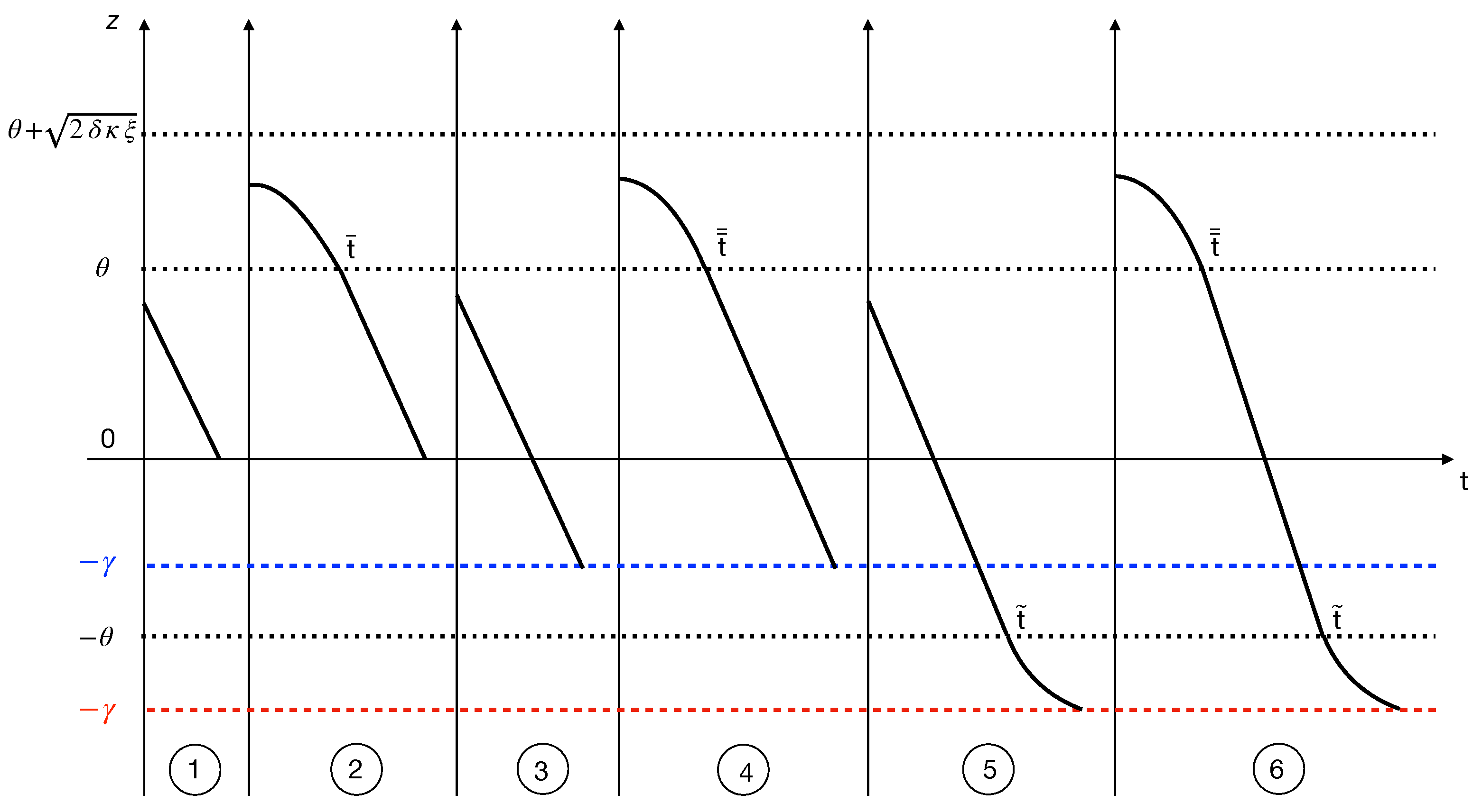
Figure 1. Summary of the graphs of the function z t in all possible instances of the problem.
Axioms 13 00300 g001
Figure 2. Numerical simulation of differential Equations (41) and (42). Parameters value: T = 2 , m 0 = 0.5 , ρ = 1 , π = 1 , δ = 1 , ξ = 0.5 , κ = 0.5 , θ = 0.2 , γ = 0.5 . Simulation with Wolfram Mathematica 12.3.
Axioms 13 00300 g002
Table 1. Profit and incentive for i-th company.
State at Time tInstantaneous ProfitState at Time TFinal Incentive
1 δ i ( π i ρ i ) 1 0
+ 1 δ i ( π i ( ρ i + ξ i ) ) + 1 γ i
Table 2. Table of variables and parameters.
VariablesDescription
X t production State of the representative player (state function)
U t transition rate of the representative player (control function)
ParametersDescription
Tfixed final time
δ instantaneous demand for the product
π selling price for one unit of goods
ρ unit production cost in the South country
ξ additional production cost in the North country
κ , θ quadratic and linear activation costs of the transition rate
γ final incentive
Table 3. Sensitivity analysis for t ¯ .
T θ δ ξ
t ¯ +++
Table 4. Sensitivity analysis for t ¯ ¯ and t ˜ .
T θ δ ξ γ
t ¯ ¯ +++
t ˜ ++++
Disclaimer/Publisher’s Note: The statements, opinions and data contained in all publications are solely those of the individual author(s) and contributor(s) and not of MDPI and/or the editor(s). MDPI and/or the editor(s) disclaim responsibility for any injury to people or property resulting from any ideas, methods, instructions or products referred to in the content.